Abstract
For a long time, the traditional injection molding industry has faced challenges in improving production efficiency and product quality. With advancements in Computer-Aided Engineering (CAE) technology, many factors that could lead to product defects have been eliminated, reducing the costs associated with trial runs during the manufacturing process. However, despite the progress made in CAE simulation results, there still exists a slight deviation from actual conditions. Therefore, relying solely on CAE simulations cannot entirely prevent product defects, and businesses still need to implement real-time quality checks during the production process. In this study, we developed a Back Propagation Neural Network (BPNN) model to predict the occurrence of short-shots defects in the injection molding process using various process states as inputs. We developed a Back Propagation Neural Network (BPNN) model that takes injection molding process states as input to predict the occurrence of short-shot defects during the injection molding process. Additionally, we investigated the effectiveness of two different transfer learning methods. The first method involved training the neural network model using CAE simulation data for products with length–thickness ratios (LT) of 60 and then applying transfer learning with real process data. The second method trained the neural network model using real process data for products with LT60 and then applied transfer learning with real process data from products with LT100. From the results, we have inferred that transfer learning, as compared to conventional neural network training methods, can prevent overfitting with the same amount of training data. The short-shot prediction models trained using transfer learning achieved accuracies of 90.2% and 94.4% on the validation datasets of products with LT60 and LT100, respectively. Through integration with the injection molding machine, this enables production personnel to determine whether a product will experience a short-shot before the mold is opened, thereby increasing troubleshooting time.
1. Introduction
In recent years, with the development of Industry 4.0, many traditional industries have been transitioning towards smart manufacturing. In the injection molding industry, the challenge of shortening product cycles has emerged. Reducing the number of trial runs can significantly enhance product development speed and reduce material costs incurred during testing. Many companies have adopted Computer-Aided Engineering (CAE) to eliminate most factors that could lead to product defects. However, CAE cannot entirely eliminate potential issues, especially the variability in actual parameters during each molding process. Therefore, when problems arise with injection parameters, reliance on the experience of on-site personnel for parameter adjustments is still necessary, and CAE cannot be used for real-time decision-making in the field. Effectively predicting product quality using informative data is a significant topic in today’s era of smart manufacturing.
In the relevant literature on injection molding, Gotlih et al. [1] mentioned that process parameters affect product quality, cycle time, and production costs in the manufacturing process. Therefore, finding optimized process parameters is a crucial process. Mathivanan et al. [2] emphasized the importance of optimizing injection parameters for product quality, and mentioned that iteratively changing processing parameters to improve product defects consumes a significant amount of time, material, and manpower. They proposed using the Taguchi Methods to identify injection parameters that cause shrinkage defects in products. The results show that this technique effectively reduces shrinkage defects in products under different injection parameters. Huang et al. [3] discussed the parameters that cause warping in transmission parts of Flapping-Wing Micro-Aerial Vehicles (FW-MAV), including injection temperature, mold temperature, injection pressure, and holding time. They used the Taguchi Methods to find the optimal process parameters and validated the results through CAE system analysis and simulation. The findings demonstrate that these optimized process parameters minimized warping in the products. Zhao et al. [4] highlighted how CAE systems can optimize mold structures and modify problematic injection parameters before production, thus avoiding the cost of repeated testing in actual production. This technology not only shortens mold development cycles, but also reduces unnecessary human and material resources, lowering production costs and enhancing product quality. Hentati et al. [5] discussed how residual stresses can impact the presence of defects in final products. They proposed using the Taguchi Methods to identify the process parameters that have the most significant effect on shear force in PC/ABS mixtures. Through CAE simulations and verification, the Taguchi Methods were able to identify optimized process parameters that resulted in PC/ABS products with good shear stress characteristics and no defects, effectively enhancing the quality of injection-molded products.
In the machine learning literature, Kwak et al. [6] used CAE simulation results as training data to train a neural network model for predicting the porosity generation ratio and volume deformation of plastic optical lenses based on the injection molding process parameters. They demonstrated the feasibility of this method through actual experiments. Shen et al. [7] mentioned that injection molding process parameters have a significant impact on product quality. They proposed a model architecture that combines artificial neural networks with genetic algorithms. This approach utilizes backpropagation neural networks to handle the nonlinear relationship between process parameters and product quality. Additionally, genetic algorithms are employed for optimizing the model’s process parameters. The results show that the combination of backpropagation neural networks and genetic algorithms effectively improved the product’s volume shrinkage. Denni et al. [8] proposed the use of the Taguchi Methods, Back Propagation Neural Network (BPNN), a hybrid Particle Swarm Optimization (PSO), and Genetic Algorithm (GA) to identify optimized process parameters. The results demonstrate that this approach not only enhances the quality of plastic products, but also effectively reduces process variations. Denni also pointed out that the Back Propagation Neural Network can face challenges such as overfitting due to poor initial link values or excessive training iterations, making it difficult to find the best solution. Therefore, they used Genetic Algorithms to address this issue and increase prediction accuracy. Bruno et al. [9] mentioned that in order to prevent the delivering of defective products to customers and incurring unpredictable costs, they proposed the use of classification models based on Artificial Neural Networks (ANN) and Support Vector Machines (SVM). The results show that these models accurately classify product quality, whether it is related to short-shots, incomplete filling, burn marks, warping, or flash, into different categories. Alberto et al. [10] emphasized the significance of optimizing process parameters for improving product quality. Even when process parameters are adjusted to their optimum settings, variations in material properties and machine instability can still impact product quality. Using machine learning enables the effective monitoring of process parameters during product production and allows for rapid adjustments to improve product quality. Mohammad et al. [11] discussed how to accurately bring the weight of injection-molded products close to the ideal weight and reduce process time. Optimizing process parameters is one of the most crucial steps in achieving this. Therefore, they proposed a model architecture that combines artificial neural networks and genetic algorithms. The results demonstrate that this technique can accurately identify optimized process parameters, effectively reducing process time, and bringing the final product weight closer to the ideal weight. Yin et al. [12] mentioned that mold temperature, melt temperature, holding pressure, holding time, and cooling time are important parameters affecting warpage deformation. They proposed a Back Propagation Neural Network architecture with two hidden layers, each containing 20 neurons, to predict warpage deformation based on these five parameters. The network was trained using finite element analysis data, and the results show that this system had a prediction error of within 2%, effectively optimizing process parameters and reducing warpage deformation. Matthias et al. [13] mentioned that identifying the optimal machine setting parameters in the injection molding process can be time-consuming and costly in terms of trial runs. Therefore, they proposed a regression model based on an artificial neural network for injection molding. The input parameters included injection weight, screw position, material properties, and plasticization time, while the output parameters were screw speed and back pressure. The results show that using unseen data for prediction yielded an average error of 0.27% with a standard deviation of 0.37%. This approach reduces the time and trial run costs associated with the process stage. Tsai et al. [14] proposed a model architecture that combines an Artificial Neural Network (ANN) with Genetic Algorithms (GA). This approach effectively reduced warping in optical lenses and utilized the Taguchi Methods to identify the optimal injection parameters. They found that the factors affecting product warping were mold temperature, cooling time, holding pressure, and holding time. The results show that this method improved the shape accuracy of the lenses by 13.36%. Yang et al. [15] proposed an optimization approach for the injection molding process of automobile front frames, utilizing a regression equation, genetic algorithms, and Back Propagation Neural Networks. Five input parameters, namely, mold temperature, melt temperature, holding pressure, injection time, and holding time, were used, and the output parameters were volume shrinkage and warpage. The results indicate that this method achieved the optimization of volume shrinkage and warpage for automobile front panels, leading to an improvement in product quality and a reduction in production costs.
In the literature on transfer learning, Hasan et al. [16] proposed a neural network model using six parameters as input values—injection time, holding pressure, holding time, mold temperature, cooling time, and melt temperature—to predict product weight. They used simulated data for training and then employed transfer learning to retrain the neural network model with real data. The results show that transfer learning accelerated the network’s learning process compared to training from scratch. It also improved the accuracy of the model’s predictions while overcoming the challenges of limited real experimental data and high trial run costs. Chai et al. [17] introduced a deep probabilistic transfer regression framework designed to address the issue of missing data in data-driven soft sensors. This framework transfers source domain conditions to the target domain. After validation through various models, the results demonstrated the effectiveness of this approach in handling missing data issues in the target domain and improving the performance of soft sensors. Zhou et al. [18] introduced a Long Short-Term Memory Car-Following (LSTM CF) model for Adaptive Cruise Control (ACC) constructed through transfer learning. This model transfers knowledge from the source domain of Human-Driving Vehicles (HV) to the target domain of ACC. They also mentioned that a small amount of ACC data can be used to build highly accurate models. The results indicate that transfer learning is not only an effective approach for modeling with limited data, but also enhances model accuracy. Muneeb et al. [19] mentioned that transfer learning enhances model accuracy. They utilized a large population’s genetic data to understand Single-Nucleotide Polymorphisms (SNPs) causing diseases and then transferred this knowledge to predict genotypes and phenotypes in smaller populations. The results show an improvement in model prediction accuracy ranging from 2% to 14.2%. Huang et al. [20] mentioned that while CAE analysis helps address some issues affecting injection-molded products, on-site adjustments of parameters still rely on human expertise. Therefore, they proposed a Back Propagation Neural Network (BPNN) network model and used CAE simulation data as the training data. The inputs included melt temperature, mold temperature, injection speed, holding pressure, and holding time, while the outputs included EOF pressure, maximum cooling time, Z-axis warpage, X-axis shrinkage, and Y-axis shrinkage. They then retrained the model using real machine data through transfer learning. The results showed higher accuracy compared to conventional network models.
2. Background Knowledge
2.1. Computer Aided Engineering (CAE)
With the advancement of computer technology, Computer-Aided Engineering (CAE) has become a valuable technique in many engineering industries for addressing practical problems. It involves using computers to simulate and analyze the product manufacturing process, enabling the identification of design flaws before actual production, and assessing the feasibility of product designs. As illustrated in Figure 1, in the injection molding industry, before conducting CAE simulations of the product manufacturing process, in addition to providing the three-dimensional model of the product, it is necessary to configure a series of prerequisites. These prerequisites primarily fall into three categories: material parameters, process parameters, and analysis sequence.
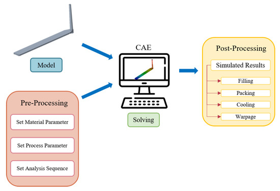
Figure 1.
CAE analysis process.
In configuring material parameters, determining material properties such as viscosity, PVT (pressure–volume–temperature) relationships, specific heat, and thermal conductivity is crucial. As for configuring process parameters, this involves setting up molding conditions, including injection speed, injection position, injection pressure, holding pressure, cooling time, and more. In the context of analysis sequence, settings include mold gate position, water channel location, and simulation grid size. By configuring these parameters, simulation results can closely approximate real-world scenarios, thereby enhancing the accuracy and reliability of the simulation.
Utilizing Computer-Aided Engineering to simulate and rectify defects before production significantly reduces product development cycles, material, and labor costs associated with trial runs, while simultaneously improving overall production efficiency.
2.2. Back Propagation Neuron Network (BPNN)
Back Propagation Neural Network (BPNN), also known as Multilayer Perceptron, is a type of feedforward neural network belonging to supervised learning. It operates on the concept of gradient descent and adjusts the weights and biases of each node through backward propagation until the output values closely match the desired values, as illustrated in Figure 2. The structure of the Back Propagation Neural Network primarily consists of three layers, as described below:
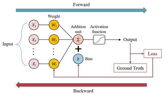
Figure 2.
Back Propagation Neural Network training process diagram.
- Input Layer
The input data are received through this layer and serve as input to the neural network. The nodes in this layer do not perform computations; typically, the received data are preprocessed here before being forwarded to the next layer.
- Hidden Layer
A neural network can have more than one hidden layer, and the number of hidden layers and the number of neurons in each layer are set based on the specific problem requirements. When there are more hidden layers, the network’s computational complexity and time consumption increase. There is no one-size-fits-all standard for the number of hidden layers and neurons, and typically, a trial-and-error process is used to adjust and find the optimal configuration, often guided by learning and validation curves.
- Output Layer
This layer receives the output computed by the hidden layers, and the form of the output in the output layer depends on the model’s task. In binary classification problems, the output layer typically contains one neuron, while in multi-class classification problems, the output layer usually contains several neurons, with each neuron corresponding to a category. The output in the output layer is often processed using an activation function to obtain the final prediction of the model. Common activation functions include Softmax, ReLU, Tanh, and Sigmoid functions.
2.3. Data Preprocessing
Prior to training the neural network, the preprocessing of the training data is a crucial step. Handling missing values, eliminating irrelevant variables, and standardizing data are essential in order to improve the learning of the model. Among the various parameters used as inputs for training the model, the values of injection pressure and injection velocity are presented in an in array format. Transforming these two sets of data into hundreds of inputs would overly complicate the model, extend training time, and require a vast amount of training data. In this study, injection pressure and injection velocity arrays were divided into three sub-arrays each, and the low and high values within each sub-array were selected as new input parameters. This reduced the original 71 input points to just 6 input points, as illustrated in Figure 3.
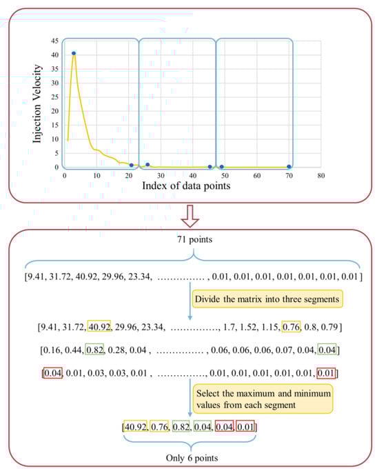
Figure 3.
Injection velocity array processing workflow.
2.4. Correlation Analysis
In many machine learning applications in injection molding research, models’ inputs are typically determined empirically. This involves using individual experiences to assess which features are more correlated with data label and selecting them as inputs for the model. However, this approach may result in a decrease in the model’s accuracy, as it could overlook other relevant features or mistakenly include features with lower correlation as the model’s inputs. Therefore, in the training process of machine learning, it is crucial to analyze the correlation between each feature and data label in a scientific manner to identify suitable combinations of input features. This method can simplify and expedite the training process of machine learning, ultimately enhancing the accuracy of the neural network model.
In this study, we will calculate the Pearson correlation coefficient between each feature (X) and the data label (Y) as a criterion to assess the correlation between them. The calculation method is as shown in function (1). The Pearson correlation coefficient is primarily used to measure the linear correlation between two sets of data. A higher absolute value of the Pearson correlation coefficient indicates a stronger correlation between the two sets. Table 1 shows the Pearson correlation coefficient between each feature and data label. In the selection of model inputs, we will set a correlation coefficient threshold to filter model inputs. If the Pearson correlation coefficient between a particular feature and data label is higher than the threshold, it will be chosen as a model input. In Figure 4, to determine a suitable threshold, we have established an initial model, and selected model inputs based on different threshold values. The CAE data were split into a training set and a validation set with an 8:2 ratio. Finally, we compared the performance of trained models with different threshold values on the validation set to guide our selection. Ultimately, this study chose a threshold of 0.04 for filtering model inputs.

Table 1.
The absolute values of correlation coefficients for each input parameter.
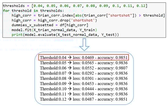
Figure 4.
Pearson product–moment correlation coefficient threshold validation.
2.5. Transfer Learning
In this study, through layer transfer, when loading a pre-trained model, the pre-trained weights are loaded without loading the original model’s input and output layers. During training, all pre-trained layers can be set as non-trainable and their weights are frozen, or one can only select specific layers to be set as non-trainable, and freeze their weights. The code is shown in Figure 5, and the process is illustrated in Figure 6. The purpose is to prevent the originally trained weights from being updated and to ensure that the pre-trained weights are not disrupted during the training of the new model. Next, new hidden layers and output layers are added to create a new prediction model, and the training parameters for the new model are compiled. Finally, new training data are loaded for secondary training.
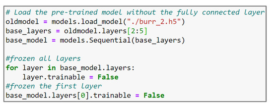
Figure 5.
Code for Freezing Pre-trained Hidden Layers.
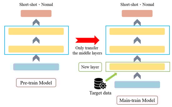
Figure 6.
Transfer learning process diagram.
3. Methodology
As shown in Figure 7, this study collected and verified molding data using two types of long flat plate molds, with LT60 (length 120 mm, width 15 mm, thickness 2 mm) and LT100 (length 200 mm, width 15 mm, thickness 2 mm), respectively. ABS POLYLAC® PA-756 was selected as the material for the products. Mold filling simulations were performed using the CAE analysis software Moldex3D (version 2023 R2) under different injection parameter settings for the LT60 long flat plate mold. These simulated data were then used as training data, with the product’s short-shot condition as the label, to train the model.
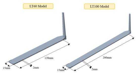
Figure 7.
The dimensions of the long flat plate.
After obtaining the pre-trained model, we used the SM-120T Horizontal Injection Molding Machine from Hundred Plastics to perform actual molding of the LT60 long flat plate mold to acquire real filling data. This dataset was used for transfer learning with the pre-trained model. Additionally, we used the actual filling data of the LT60 long flat plate mold to obtain the pre-trained model, and then performed transfer learning using the actual filling data of the LT100 long flat plate mold. Finally, we will evaluate the effectiveness of these two transfer learning approaches.
3.1. Transfer Learning of CAE Pre-trained Model
This study employs a transfer approach involving both virtual analysis and real-world molding. Initially, a neural network model is trained using CAE simulation data for the LT60 long flat plate model. Subsequently, transfer learning of the network model is conducted using data obtained from actual injection molding experiments. This ensures that the transferred neural network model is suitable for real-world machine predictions. During the transfer learning process, because the same model is used for secondary training, the data from actual injection molding experiments should closely resemble or match the simulated data. A significant disparity in data may result in suboptimal transfer learning outcomes and potentially impact the accuracy of the final predictive model applied to actual scenarios. The process flow is illustrated in Figure 8.
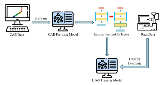
Figure 8.
Process flowchart for transfer learning of the CAE pretrained model.
In the analysis software Moldex3D’s simulation data, the main varying parameters are injection speed, holding pressure, holding time, material temperature, and mold temperature. When adjusting the parameters, the default values provided by Moldex3D are primarily used as reference. Analyzing different parameter combinations, a total of 3366 simulation data points were generated, with a ratio of 4:6 between short-shots and non-short-shots. After data preprocessing and correlation analysis, the input for the pre-trained model consisted of 20 feature parameters, and the output was used to indicate whether a short-shot occurred. The data were split into 80% training data and 20% testing data, with an additional 20% taken from the training data for validation. The model architecture consisted of 2 hidden layers, with 36 neurons in the first layer and 20 neurons in the second layer. To prevent overfitting during model training, dropout regularization was applied after both hidden layers, with a dropout rate of 0.2 for each layer. The model architecture is illustrated in Figure 9. Regarding hyperparameter settings, the learning rate was set to 0.002, ReLU and Sigmoid activation functions were used for respective layers, the optimizer was Adam, the batch size was set to 33, and the number of epochs was set to 340. The hyperparameter settings are summarized in Table 2.
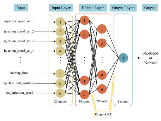
Figure 9.
CAE training model architecture.
Table 2.
CAE model hyperparameter configuration.
In the selection of hidden layers for the transfer learning model, five different transfer methods were employed to train the transfer learning model, and the results of each method were compared. The methods were as follows:
- Transfer and freeze the two hidden layers of the pre-trained model, training only the third hidden layer of the new model;
- Transfer the two hidden layers of the pre-trained model, and freeze the weight values of the first hidden layer, training only the second and third hidden layers of the new model;
- Transfer the two hidden layers of the pre-trained model and freeze the weight values of the second hidden layer, training only the first and third hidden layers of the new model;
- Transfer and freeze the first hidden layer of the pre-trained model, training only the second and third hidden layers of the new model;
- Transfer and freeze the second hidden layer of the pre-trained model, training only the first and third hidden layers of the new model.
As shown in Figure 10, during the training process of the first, second, third, and fourth transfer learning methods, the model’s loss exhibited a clear decreasing trend in the training set (blue line). However, there was a simultaneous increase in the validation set (green line), indicating the occurrence of overfitting during the training process. In contrast, for the fifth transfer learning method, the model’s loss showed a noticeable decrease in both the training and the validation set, with minimal differences between them. This suggests that the model possessed good generalization capabilities. Therefore, this study employed the fifth method for transfer learning.
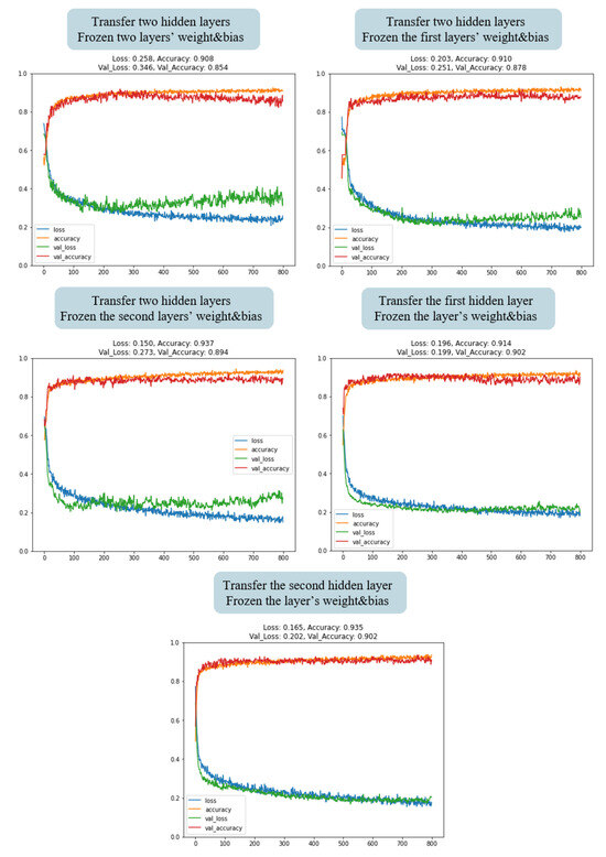
Figure 10.
Training results of LT60 model with different hidden layer transfers.
After the above validation, we selected the fifth hidden layer transfer method to build the transfer learning model. The architecture consisted of 3 hidden layers, with the first hidden layer having 36 neurons, the second hidden layer using the transferred hidden layer from the pre-trained model, and the third hidden layer having 25 neurons. Dropout regularization was applied to all hidden layers with a dropout rate of 0.3 to prevent overfitting. The weights of the transferred second hidden layer were frozen to preserve the pre-trained weights. The model architecture is shown in Figure 11. In terms of hyperparameter settings, the learning rate was set to 0.001. The activation functions for the layers awerere as follows: the first layer used Tanh, while the second and third layers used Sigmoid. The optimizer used was Adam for hyperparameter optimization. The batch size was set to 33, and the number of training iterations was set to 800. The hyperparameter settings for the model are summarized in Table 3.
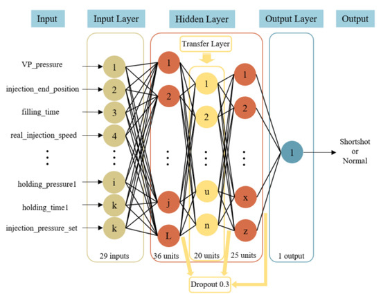
Figure 11.
LT60 transfer learning model architecture.
Table 3.
LT60 transfer learning model hyperparameter settings.
In the actual injection molding model training, 1358 data points obtained from experiments were used. After data preprocessing, the data were divided into 1100 training data points, 122 validation data points, and 136 test data points. The accuracy of the trained model applied to the training set was 93.5%, and when applied to the validation set, it was 90.2%, as shown in Figure 12. If these data were to be directly used for model training, the model architecture would be the same as the original model’s architecture. However, during the model training process, overfitting would occur, as shown in Figure 13. Therefore, more training data would be needed to enable the model to converge effectively and achieve an accuracy of over 90%.
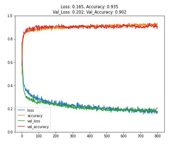
Figure 12.
Training and validation results of the LT60 transfer learning model.
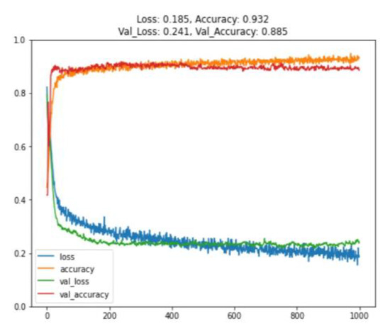
Figure 13.
Training and validation results of the LT60 model (without transfer learning).
3.2. Transfer Learning of LT60 Pre-trained Model
Training a backpropagation neural network requires a large amount of data, and obtaining a substantial volume of actual injection molding data can be challenging. Therefore, in this study, we leveraged a pre-trained LT60 network prediction model, trained with actual injection molding data, to conduct secondary training using a small amount of the LT100 data obtained. This approach effectively reduces the training time and the time required to acquire training data. The process is illustrated in Figure 14.
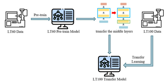
Figure 14.
LT60 pretrained model transfer learning process diagram.
We used 2050 points of actual injection data of the LT60 long plate model to train the pre-trained model. In the dataset, the ratio of short-shots to non-short-shots was 4:6. After data preprocessing and correlation analysis, the input for the pre-trained model consisted of 31 feature parameters, and the output was used to indicate whether a short-shot occurred. The data were split into 80% training data and 20% testing data, with an additional 20% taken from the training data for validation. The model architecture consisted of 3 hidden layers: the first layer had 18 neurons, the second layer had 10 neurons, and the third hidden layer had 12 neurons. Dropout regularization was applied after each hidden layer with a dropout rate of 0.3. The model’s structure is depicted in Figure 15. Regarding hyperparameter settings, the learning rate was set to 0.001. The activation functions for each layer were as follows: the first layer used Tanh, while the second and third layers used Sigmoid. Adam optimizer was employed for hyperparameter optimization. The batch size for training was set to 32, and the model was trained for 1000 epochs. The hyperparameter settings for the model are outlined in Table 4.
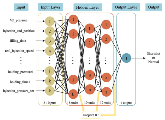
Figure 15.
LT60 pre-trained model architecture.
Table 4.
LT60 pre-trained model hyperparameter settings.
In the selection of hidden layers for the LT100 transfer learning model, ten different methods were employed to train the transfer learning model, and the results of each method were compared. The methods were as follows:
- Transfer and freeze all three hidden layers of the pre-trained model;
- Transfer the three hidden layers of the pre-trained model, and freeze the weights of the first hidden layer, then only train the second and third hidden layers of the new model;
- Transfer the three hidden layers of the pre-trained model, and freeze the weights of the second hidden layer, then only train the first and third hidden layers of the new model;
- Transfer the three hidden layers of the pre-trained model, and freeze the weights of the third hidden layer, then only train the first and second hidden layers of the new model;
- Transfer the three hidden layers of the pre-trained model, and freeze the weights of the first and second hidden layers, then only train the third hidden layer of the new model;
- Transfer the three hidden layers of the pre-trained model, and freeze the weights of the first and third hidden layers, then only train the second hidden layer of the new model;
- Transfer the three hidden layers of the pre-trained model, and freeze the weights of the second and third hidden layers, then only train the first hidden layer of the new model;
- Transfer and freeze the first hidden layer of the pre-trained model, and only train the second and third hidden layers of the new model;
- Transfer and freeze the second hidden layer of the pre-trained model, then only train the first and third hidden layers of the new model;
- Transfer and freeze the third hidden layer of the pre-trained model, then only train the first and second hidden layers of the new model.
As shown in Figure 16, from the training results, it can be observed that when using the first, fifth, and sixth transfer learning methods, the model’s loss in the training set (blue line) and validation set (green line) exhibited a gradual decreasing trend. However, there remained a significant gap between the two, and this gap did not show a tendency to diminish with increasing training iterations. This indicates that the model was likely to experience overfitting as the number of training iterations increased. In the cases of the second, third, fourth, seventh, eighth, and tenth methods, although the model’s loss in the training set decreased noticeably, the model’s loss in the validation set increased, indicating the occurrence of overfitting in the training process. The training process of the ninth transfer learning method revealed a noticeable decrease in both training and validation set losses, with a simultaneous reduction in the gap between them. This indicates that the model exhibited excellent generalization capabilities. Therefore, we have selected the ninth method for transfer learning in this study.
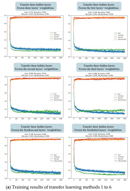
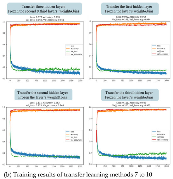
Figure 16.
Training results of LT100 model with different hidden layer transfers. (a) Training results of transfer learning methods 1 to 6; (b) Training results of transfer learning methods 7 to 10.
Following the above validation, we selected the ninth hidden layer transfer method to build the transfer learning model. Its architecture consisted of 3 hidden layers. The first layer had 18 neurons, the second hidden layer used the second hidden layer of the LT60 pre-trained model, and the third hidden layer had 12 neurons. We applied regularization dropout to each hidden layer, with a dropout rate of 0.3, and froze the weights of the transferred second hidden layer to prevent the trained weights from being disrupted. The model architecture is illustrated in Figure 17. In terms of hyperparameter settings, the learning rate was set to 0.001. The activation functions for the first and third layers were Tanh and Sigmoid, respectively. Adam was employed as the optimizer for hyperparameter optimization. The batch size was set to 32, and the model was trained for 2000 epochs. The hyperparameter settings for the model are detailed in Table 5.
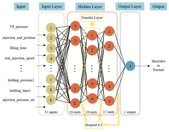
Figure 17.
LT100 transfer learning model architecture.
Table 5.
LT100 transfer learning model hyperparameter settings.
In the training of the LT100 transfer learning model, we used 900 data points obtained from experiments. After preprocessing the data, they were divided into 576 training samples, 144 validation samples, and 180 test samples. The trained model achieved a training accuracy of 96.2% and a validation accuracy of 94.4%, as shown in Figure 18. If we were to directly train a model with the same architecture using only these 900 data points, overfitting would occur due to the limited dataset, as depicted in Figure 19. Therefore, acquiring more training data is necessary to ensure effective convergence and achieve an adequate level of accuracy in the model.
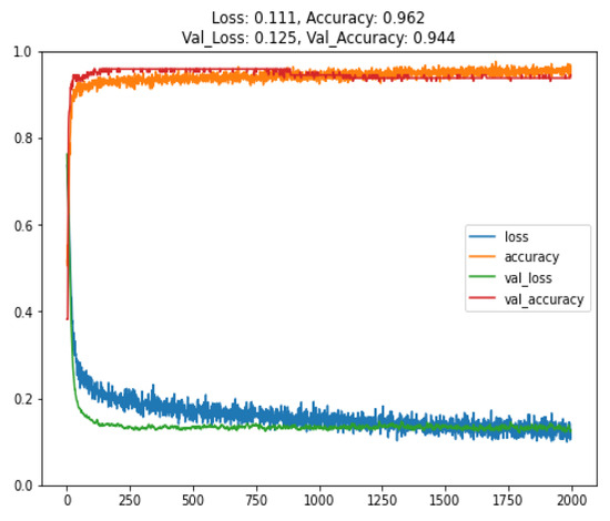
Figure 18.
Training and validation results of the LT100 transfer learning model.
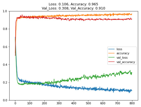
Figure 19.
Training and validation results of the LT100 model (without transfer learning).
3.3. Model’s Performance Comparative
Table 6 presents the comparative results of model performance, indicating that in both LT60 and LT100 short-shot prediction tasks, the performance of the transfer learning models surpassed that of the models without transfer learning. This suggests that utilizing transfer learning enhances the model’s performance in short-shot prediction tasks. The results underscore the potential use of transfer learning in improving model generalization and efficiency in the context of short-shot prediction tasks.
Table 6.
Comparison of the models’ performance.
3.4. Verification
In the final stage, this study integrated the trained LT100 transfer learning model with the injection molding machine to establish a real-time short-shot prediction system; the overall architecture is illustrated in Figure 20. In each production process, the system collected real-time process data, and during the cooling stage of the product, utilized these data as the model’s input to predict whether the product will experience short-shot. The total duration of the LT100 product’s overall process was 16 s, with 1 s allocated to the product filling time, and the remaining 15 s dedicated to product cooling. In contrast to traditional quality inspection methods such as AOI (Automated Optical Inspection), which requires inspection after the product has cooled and been removed from the mold, the integrated application of the model proposed in this study with the injection molding machine enabled the detection of short shots at only 6.25% of the overall process execution. This allows personnel to initiate the defect troubleshooting process earlier, thereby enhancing production efficiency.

Figure 20.
Real-time short-shot prediction system operation process.
4. Discussion
This study utilized transfer learning to perform secondary training on pre-trained neural network models using a limited amount of data, resulting in new neural network prediction models. The use of transfer learning significantly improved prediction accuracy compared to models that did not employ transfer learning. The original LT60 and LT100 models had validation accuracies of 88.5% and 91%, and overfitting occurred during training. However, the LT60 and LT100 transfer models with limited data achieved validation accuracies of 90.2% and 94.4%, respectively. This approach not only reduces the time and material costs of acquiring training data, but also enhances the predictive accuracy of the products. The results of this experiment demonstrate the potential of transfer learning to reduce model training costs in the field of injection molding. By leveraging pre-trained neural network models, effective secondary training can be conducted with limited data, leading to significant savings in time and resources while substantially enhancing the predictive performance of the model. In addition, through the integrated application of the model with an injection molding machine, personnel can instantly determine whether short-shots have occurred in the product as soon as the filling process is completed. There is no need to wait until the product has cooled down to perform the inspection, allowing the defect troubleshooting process to be initiated earlier, thereby enhancing overall production efficiency.
In the future, further explorations can be done to investigate the effectiveness of transferring the model trained for predicting short-shots to predicting models for other types of product defects, expanding the application scope of transfer learning.
Author Contributions
Conceptualization, Z.-W.Z., H.-Y.Y. and Y.-H.T.; methodology, Z.-W.Z., H.-Y.Y. and B.-X.X.; software, Z.-W.Z., H.-Y.Y. and B.-X.X.; validation, B.-X.X., Y.-H.T., S.-C.C. and W.-R.J.; investigation, Y.-H.T., S.-C.C. and W.-R.J.; data curation, Z.-W.Z. and H.-Y.Y.; writing—original draft preparation, H.-Y.Y.; writing—review and editing, Z.-W.Z.; visualization, Z.-W.Z., H.-Y.Y. and B.-X.X.; supervision, Y.-H.T., S.-C.C. and W.-R.J. All authors have read and agreed to the published version of the manuscript.
Funding
This research received no external funding.
Institutional Review Board Statement
Not applicable.
Informed Consent Statement
Not applicable.
Data Availability Statement
The data are not publicly available due to subsequent research needs.
Conflicts of Interest
The authors declare no conflict of interest.
References
- Gotlih, J.; Brezocnik, M.; Pal, S.; Drstvensek, I.; Karner, T.; Brajlih, T. A Holistic Approach to Cooling System Selection and Injection Molding Process Optimization Based on Non-Dominated Sorting. Polymers 2022, 14, 4842. [Google Scholar] [CrossRef] [PubMed]
- Mathivanan, D.; Nouby, M.; Vidhya, R. Minimization of sink mark defects in injection molding process—Taguchi approach. Int. J. Eng. Sci. Technol. 2010, 2, 13–22. [Google Scholar] [CrossRef]
- Huang, H.Y.; Fan, F.Y.; Lin, W.C.; Huang, C.F.; Shen, Y.K.; Lin, Y.; Ruslin, M. Optimal Processing Parameters of Transmission Parts of a Flapping-Wing Micro-Aerial Vehicle Using Precision Injection Molding. Polymers 2022, 14, 1467. [Google Scholar] [CrossRef] [PubMed]
- Zhao, Z.; He, X.; Liu, M.; Liu, B. Injection Mold Design and Optimization of Automotive panel. In Proceedings of the 2010 Third International Conference on Information and Computing, Wuxi, China, 4–6 June 2010; pp. 119–122. [Google Scholar]
- Hentati, F.; Hadriche, I.; Masmoudi, N.; Bradai, C. Optimization of the injection molding process for the PC/ABS parts by integrating Taguchi approach and CAE simulation. Int. J. Adv. Manuf. Technol. 2019, 104, 4353–4363. [Google Scholar] [CrossRef]
- Kwak, T.S.; Suzuki, T.; Bae, W.B.; Uehara, Y.; Ohmori, H. Application of Neural Network and Computer Simulation to Improve Surface Profile of Injection Molding Optic Lens. J. Mater. Process. Technol. 2005, 70, 24–31. [Google Scholar] [CrossRef]
- Shen, C.; Wang, L.; Li, Q. Optimization of Injection Molding Process Parameters Using Combination of Artificial Neural Network and Genetic Algorithm Method. J. Mater. Process. Technol. 2007, 183, 412–418. [Google Scholar] [CrossRef]
- Denni, K. An Integrated Optimization System for Plastic Injection Molding Using Taguchi Method, BPNN, GA, and Hybrid PSO-GA. Ph.D. Thesis, Chung Hua University, Taiwan, China, 2004. [Google Scholar]
- Bruno, S.; Joao, S.; Guillem, A. Machine Learning Methods for Quality Prediction in Thermoplastics Injection Molding. In Proceedings of the 2021 International Conference on Electrical, Computer and Energy Technologies, Cape, South Africa, 16–17 November 2023; pp. 1–6. [Google Scholar]
- Alberto, T.; Ramón, A. Machine Learning algorithms for quality control in Plastic Molding Industry. In Proceedings of the 2013 IEEE 18th Conference on Emerging Technologies & Factory Automation, Cagliari, Italy, 10–13 September 2013; pp. 1–4. [Google Scholar]
- Mohammad, S.M.; Abbas, V.; Fatemeh, S. Optimization of Plastic Injection Molding Process by Combination of Artificial Neural Network and Genetic Algorithm. J. Optim. Ind. Eng. 2013, 13, 49–54. [Google Scholar]
- Yin, F.; Mao, H.; Hua, L.; Guo, W.; Shu, M. Back Propagation neural network modeling for warpage prediction and optimization of plastic products during injection molding. Mater. Des. 2011, 32, 1844–1850. [Google Scholar] [CrossRef]
- Matthias, S.; Dominik, A.; Georg, S. A Simulation-Data-Based Machine Learning Model for Predicting Basic Parameter Settings of the Plasticizing Process in Injection Molding. Polymers 2021, 13, 2652. [Google Scholar]
- Tsai, K.M.; Luo, H.J. An inverse model for injection molding of optical lens using artificial neural network coupled with genetic algorithm. J. Intell. Manuf. 2017, 28, 473–487. [Google Scholar] [CrossRef]
- Yang, K.; Tang, L.; Wu, P. Research on Optimization of Injection Molding Process Parameters of Automobile Plastic Front-End Frame. Adv. Mater. Sci. Eng. 2022, 2022, 5955725. [Google Scholar] [CrossRef]
- Hasan, T.; Alexandro, G.; Julian, H.; Thomas, T.; Christian, H.; Tobias, M. Transfer-Learning Bridging the Gap between Real and Simulation Data for Machine Learning in Injection Molding. Procedia Cirp 2018, 72, 185–190. [Google Scholar]
- Chai, Z.; Zhao, C.; Huang, B.; Chen, H. A Deep Probabilistic Transfer Learning Framework for Soft Sensor Modeling With Missing Data. IEEE Trans. Neural Netw. Learn. Syst. 2022, 33, 7598–7609. [Google Scholar] [CrossRef] [PubMed]
- Zhou, J.; Wan, J.; Zhu, F. Transfer Learning Based Long Short-Term Memory Car-Following Model for Adaptive Cruise Control. IEEE Trans. Intell. Transp. Syst. 2022, 23, 21345–21359. [Google Scholar] [CrossRef]
- Muneeb, M.; Feng, S.; Henschel, A. Transfer learning for genotype–phenotype prediction using deep learning models. BMC Bioinformatics 2022, 23, 511. [Google Scholar] [CrossRef] [PubMed]
- Huang, Y.M.; Jong, W.R.; Chen, S.C. Transfer Learning Applied to Characteristic Prediction of Injection Molded Products. Polymers 2021, 13, 3874. [Google Scholar] [CrossRef] [PubMed]
Disclaimer/Publisher’s Note: The statements, opinions and data contained in all publications are solely those of the individual author(s) and contributor(s) and not of MDPI and/or the editor(s). MDPI and/or the editor(s) disclaim responsibility for any injury to people or property resulting from any ideas, methods, instructions or products referred to in the content. |
© 2023 by the authors. Licensee MDPI, Basel, Switzerland. This article is an open access article distributed under the terms and conditions of the Creative Commons Attribution (CC BY) license (https://creativecommons.org/licenses/by/4.0/).