Refined Landslide Susceptibility Mapping by Integrating the SHAP-CatBoost Model and InSAR Observations: A Case Study of Lishui, Southern China

Abstract

Landslide susceptibility mapping based on static influence factors often exhibits issues of low accuracy and classification errors. To enhance the accuracy of susceptibility mapping, this study proposes a refined approach that integrates categorical boosting (CatBoost) with small baseline subset interferometric synthetic-aperture radar (SBAS-InSAR) results, achieving more precise and detailed susceptibility mapping. We utilized optical remote sensing images, the information value (IV) model, and fourteen influencing factors (elevation, slope, aspect, roughness, profile curvature, plane curvature, lithology, distance to faults, land use type, normalized difference vegetation index (NDVI), topographic wetness index (TWI), distance to rivers, distance to roads, and annual precipitation) to establish the IV-CatBoost landslide susceptibility mapping method. Subsequently, the Sentinel-1A ascending data from January 2021 to March 2023 were utilized to derive the deformation rates within the city of Lishui in the southern region of China. Based on the outcomes derived from IV-CatBoost and SBAS-InSAR, a discernment matrix was formulated to rectify inaccuracies in the partitioned regions, leading to the creation of a refined information value CatBoost integration (IVCI) landslide susceptibility mapping model. In the end, we utilized optical remote sensing interpretations alongside surface deformations obtained from SBAS-InSAR to cross-verify the excellence and accuracy of IVCI. Research findings indicate a distinct enhancement in susceptibility levels across 165,784 grids (149.20 km²) following the integration of SBAS-InSAR correction. The enhanced susceptibility classes and the spectral characteristics of remote sensing images closely correspond to the trends of SBAS-InSAR cumulative deformation, reflecting a high level of consistency with field-based conditions. These improved classifications effectively enhance the refinement of landslide susceptibility mapping. The refined susceptibility mapping approach proposed in this paper effectively enhances landslide prediction accuracy, providing valuable technical reference for landslide hazard prevention and control in the Lishui region.

1. Introduction

Landslides are considered one of the most severe geological hazards, often characterized by the downslope movement of rock masses or soil along slopes [1], posing a significant threat to human life and property safety. In recent years, global warming and other factors have led to a surge in landslide disasters on a global scale [2], posing a substantial threat to the safety of people worldwide. Therefore, enhancing the study of landslide susceptibility holds significant practical importance for disaster mitigation and prevention [3,4].

Landslide susceptibility provides a visual representation of the spatial probability of landslide disasters in different regions. It serves as a critical tool for landslide prevention, monitoring, mitigation, and assessment in geoscience practices. Landslide susceptibility models can be broadly classified into two categories: qualitative and quantitative [5,6]. Common qualitative models include analytic hierarchy processes (AHP) [7,8] and fuzzy logic models [9]. Common quantitative models can be broadly categorized into statistical models, machine learning models, and deep learning models. Statistical models mainly include frequency ratio models [10,11], logistic regression (LR) models [11,12] and information value (IV) models [13]; machine learning models primarily consist of random forests (RF) [14,15] and support vector machines (SVM) [16,17]; deep learning models mainly encompass convolutional neural networks (CNN) [18,19] and deep neural networks (DNN) [20,21]. Traditional qualitative models are heavily influenced by subjective human factors, whereas machine learning models demonstrate better performance in handling high-dimensional nonlinear data, such as susceptibility assessment. They have yielded accurate results in susceptibility evaluations in many regions [22].

In recent years, many scholars have incorporated deep learning models into landslide susceptibility research [18,23]. These models exhibit higher accuracy compared to traditional machine learning models. However, their performance in susceptibility assessment is constrained by variations in geographical regions and landslide sample sizes. Meanwhile, ensemble machine learning models have emerged prominently in machine learning, as they mitigate overfitting risks while enhancing model accuracy and stability [24]. Ensemble machine learning models, such as Boosting, Bagging, Stacking, AdaBoost, and Gradient Boosting, have been successfully applied in the field of landslide susceptibility. Moreover, several researchers have improved the accuracy and robustness of landslide susceptibility prediction by combining predictions from multiple models. Sahin [25] successfully applied eXtreme Gradient Boosting (XGBoost) to landslide susceptibility research. Zhang et al. [26] achieved higher accuracy in landslide susceptibility assessment in the Wanzhou District by using the latest boosting ensemble algorithms, such as Light Gradient Boosting (LightGBM) and CatBoost, which efficiently address issues related to categorical features, gradient bias, and prediction shift and thus improved the algorithm’s accuracy and generalization capabilities.

With the continuous development of machine learning and deep learning algorithms, their accuracy and generalization capabilities have significantly improved. However, they remain black-box models characterized by instability and poor interpretability. In the field of landslide susceptibility, some scholars have attempted to use SHapley Additive exPlanations (SHAP) to provide explanations for machine learning models. Pradhan et al. [27] successfully elucidated the weightings of the internal features and prediction outcomes of a CNN model using SHAP. Iban et al. [28] utilized SHAP to elucidate three ensemble learning models, namely XGBoost, NGBoost, and LightGBM. The work of numerous researchers has confirmed that SHAP offers superior interpretability and visual interpretability.

Presently, landslide susceptibility assessments primarily consider large-scale static influencing factors such as elevation, slope, and lithology. Hindered by their scale and static nature, these assessments fail to capture timely and detailed susceptibility results [29]. Hence, there is a need for extensive monitoring of surface deformations to refine and amend susceptibility results, enhancing the accuracy and precision of landslide susceptibility assessments.

In recent years, with the continuous advancement and development of remote sensing technology, InSAR has been widely employed for the early detection and monitoring of landslides. The primary monitoring methods include small baseline subset interferometric synthetic-aperture radar (SBAS-InSAR), permanent scatterer interferometric synthetic-aperture radar (PS-InSAR), and differential interferometric synthetic-aperture radar (DInSAR). These diverse monitoring methods are applicable in varying situations. DInSAR utilizes SAR data at different times in the same area to obtain surface deformation information, as exemplified by Li et al. [30], who utilized DInSAR and PS-InSAR to investigate surface deformations in their study area. PS-InSAR can capture long-term surface deformations with minimal DEM and spatial–temporal baseline requirements. This makes it well-suited for monitoring urban areas with permanent scatterers, as demonstrated in recent years. For example, Amoroso et al. [31] employed PS-InSAR to assess surface deformations in the Sibari and Metaponto coastal plains and Chen et al. [32] completed the deformation monitoring of Eboling Mountain using PS-InSAR. SBAS-InSAR, capable of capturing long-term surface deformations like PS-InSAR, has lower image requirements. Additionally, it exhibits higher computational efficiency and does not necessitate a large number of permanent scatterers, as demonstrated in Zhang et al. [33]. They employed SBAS-InSAR to monitor surface deformations in the Yan’an New District. These three methods have distinct functionalities. Given that landslides often occur in non-urban hilly areas and require long-term surface deformation results, SBAS-InSAR is frequently chosen for landslide monitoring. Integrating the accurate and detailed surface deformation information obtained through SBAS-InSAR into landslide susceptibility assessment models helps address model limitations and leads to more precise results.

The integration of landslide susceptibility assessment and InSAR results has become a focal point of interest among numerous scholars. Ciampalini et al. [34] constructed a decision matrix based on landslide susceptibility classification and PS-InSAR results. By integrating the two according to different categories, they corrected some errors in susceptibility mapping. Shen et al. [35] also developed a decision matrix using susceptibility classification and PS-InSAR results, making susceptibility mapping more suitable for the southwestern karst regions. Building upon Shen’s work, Zhang et al. [36] multiplied susceptibility classification with SBAS-InSAR results and classified them based on different levels, enhancing the reliability of susceptibility mapping. Cao et al. [37] assigned different weights to landslide susceptibility and SBAS-InSAR results, multiplying them to improve the credibility of susceptibility mapping.

This study aims to address the mentioned issues by integrating extensive surface deformation monitoring into a machine learning model to rectify misclassified areas and refine landslide susceptibility mapping (LSM). The proposal involves combining synthetic-aperture radar interferometry (InSAR) with the categorical boosting (CatBoost) model to create a refined information value CatBoost integration (IVCI) susceptibility assessment model. The primary contributions and highlights include: (a) supplementing the quantity of disaster points by employing optical remote sensing imagery and traditional statistical models, thereby optimizing the selection of non-landslide points and enhancing the predictive accuracy of machine learning models; (b) introducing a novel model that combines machine learning with InSAR technology, validating its feasibility and accuracy; and (c) employing the SHAP method to interpret the model, providing intuitive insights into the importance and influence of individual features within the model.

2. Study Area and Data Preparation

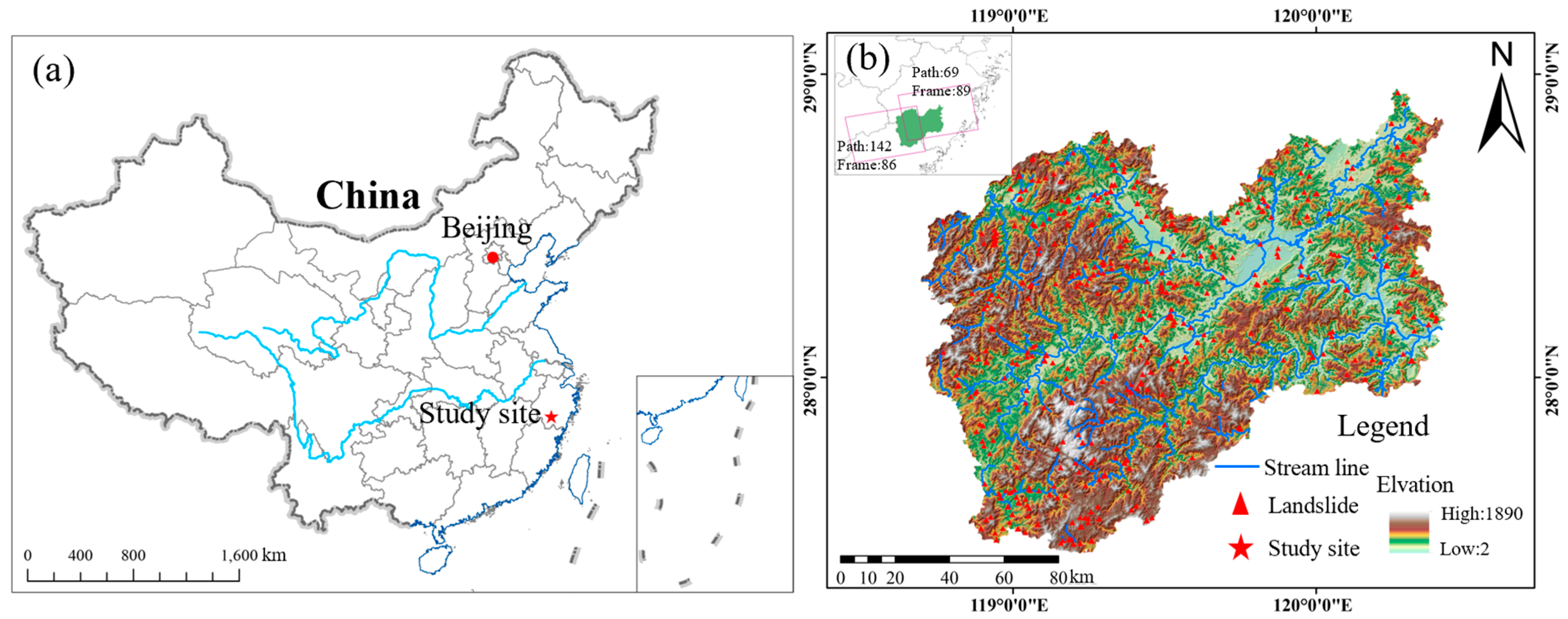
2.1. Study Area

The research area is located in Lishui (27°25′~28°57′ N, 118°41′~120°26′ E), a city in the southeast part of China, covering a total area of 17,287.13 km². The study area lies within the Zhejiang–Fujian Uplift Zone, characterized mainly by moderately mountainous and hilly terrain. Approximately 88.42% of the area is mountainous, sloping from the southwest to the northeast, with elevations ranging from 2 m to 1890 m, resulting in a relative height difference of 1888 m (Figure 1). The study area experiences a subtropical monsoon climate with an average annual temperature of 19 °C. It receives abundant rainfall, with an average annual precipitation of 1865.9 mm, with the rainy season concentrated between March and September each year.

The study area is mainly characterized by the development of Mesozoic and Paleozoic strata [38]. The Mesozoic strata comprise Middle Jurassic, Late Jurassic, and Cretaceous formations, dominated by volcaniclastic and sedimentary rocks, covering approximately 85% of the total study area. The Paleozoic rocks consist mainly of slate, schist, and mixed rock formations, with a distribution area exceeding 1200 km². Additionally, the study area is marked by the presence of two sets of fault zones. The two sets of faults are both NE oriented; one is the Lishui–Yuyao fault zone and the other is the Songyang–Pingyang fault zone. These two fault sets traverse the entire research area. The study area is prone to frequent geological hazards such as landslides, influenced by factors such as typhoons, heavy rainfall, lithology, and geological structures.

2.2. Data Preparation

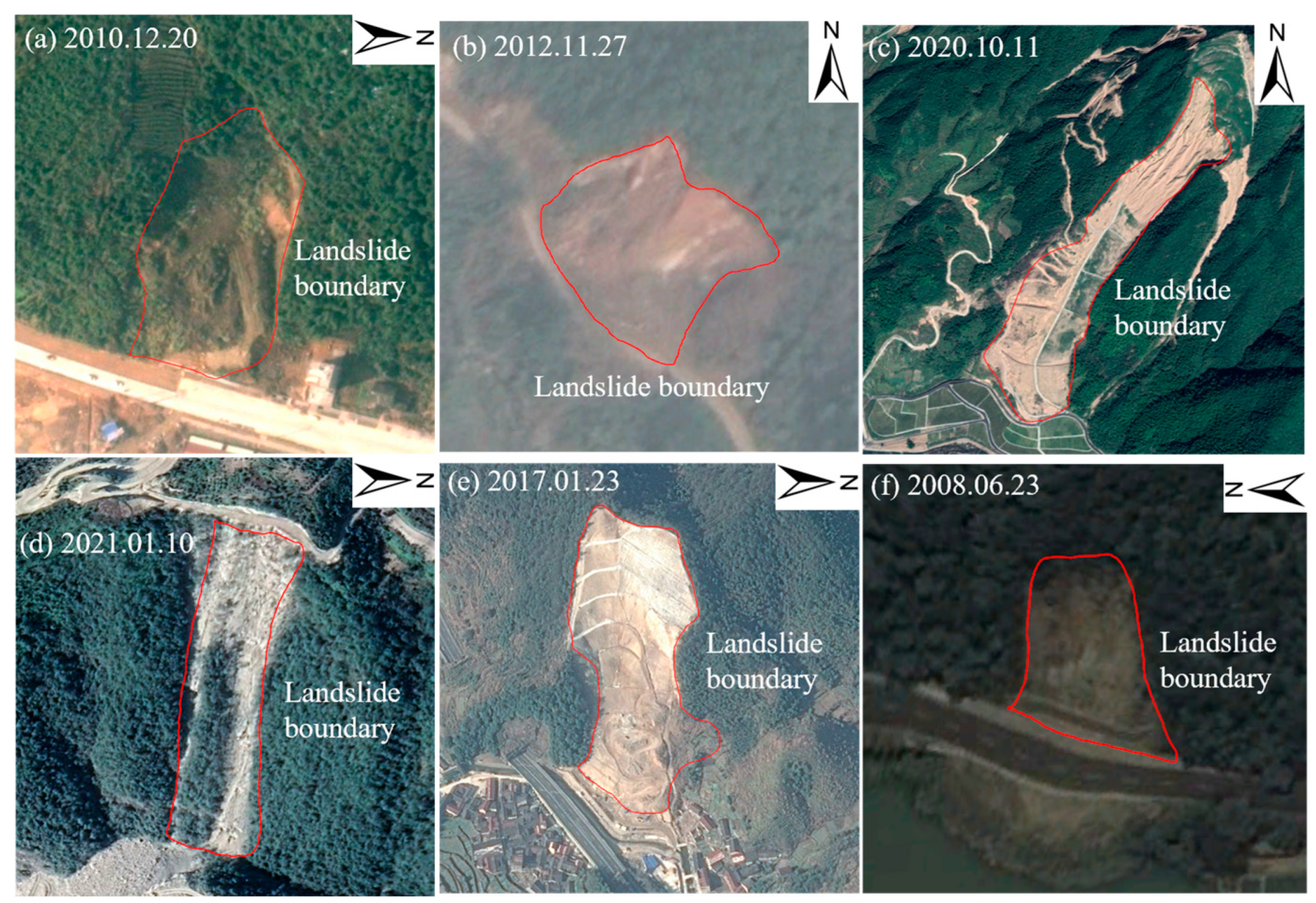
2.2.1. Landslide Dataset

This study utilized the 2021 National Geological Hazard Census Database to gather geological disaster data within the study area. Employing optical remote sensing imagery, the raw data underwent a screening process to exclude instances of collapse, debris flow, and landslides with less distinct features. This procedure resulted in the acquisition of 462 landslide data points. These points were then analyzed using optical remote sensing images. Due to the temporal gaps and resolution limitations inherent in optical remote sensing imagery, this research successfully interpreted 174 instances of landslide hazard points. The remaining 288 landslide hazard points that could not be successfully interpreted, along with the 174 successfully interpreted landslide areas, together constitute the landslide hazard database. Typical interpretation results are shown in Figure 2.

2.2.2. Impact Factor

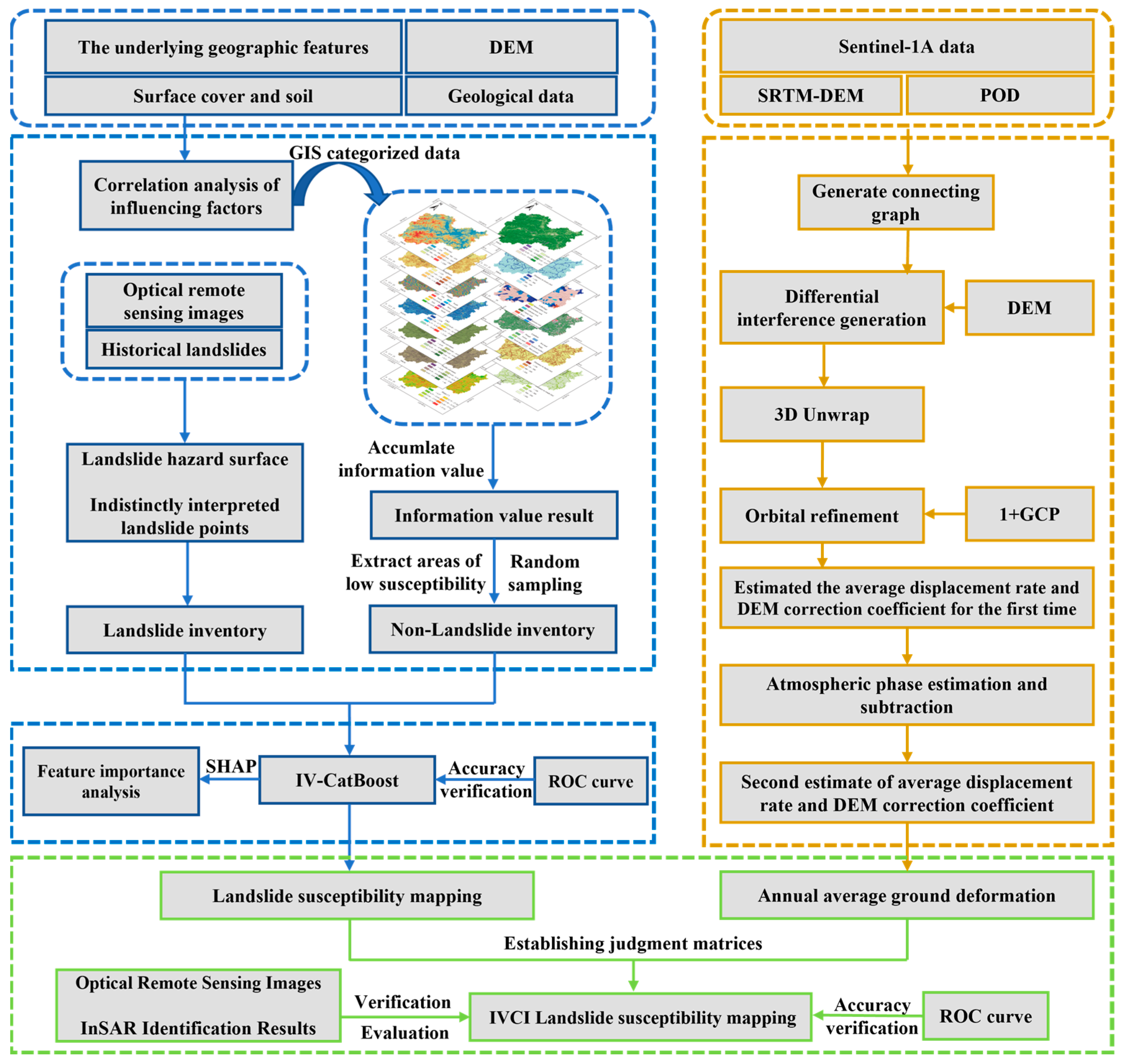
The formation of landslides is influenced by multiple factors and involves complex mechanisms. Based on the development characteristics of landslide disasters within the study area, 14 influencing factors were selected to construct the susceptibility model, including elevation, slope, aspect, roughness, profile curvature, plane curvature, lithology, distance to fault, land cover type, normalized difference vegetation index (NDVI), topographic wetness index (TWI), distance to rivers, distance to roads, and annual precipitation (Figure S1 in Supplementary Materials). Annual precipitation is derived from individual district and county statistics. Detailed data sources are listed in

Table 1. Metadata of the employed datasets.

Data Type	Source	File Type	Resolution/Scale
Terrain data	China GSCloud ASTER GDEM 30 m (https://www.gscloud.cn (accessed on 1 April 2023))	Raster	30 m
Geological data	China National Geological Archives (http://www.ngac.org.cn (accessed on 4 April 2023))	Image	1:500,000
Basic geographic information data	(open street map) OSM (https://www.openstreetmap.org (accessed on 10 April 2023))	Polyline
Environmental features	China GSCloud Landset 8 Image (https://www.gscloud.cn (accessed on 23 April 2023))	Raster	30 m
	Globe Land 30 (http://www.globallandcover.com/home.html?type=data (accessed on 3 May 2023))	Raster	30 m

. To ensure the accuracy of the data and the model, a grid cell size of 30 m by 30 m was chosen for the landslide susceptibility assessment model. The continuous data were divided into eight classes using the ArcGIS natural breaks method, while the discrete data were classified based on their inherent attributes. Refer to Figure S1 in Supplementary Materials and

Table 2. Results of IV values and influencing factors.

Impact Factor	Type of Data	Class	Number Classified	Information Value
Elevation (m)	Continuous Data	<228	2,278,531	0.06201
		228~388	3,191,332	0.38988
		388~542	3,274,549	0.49857
		542~700	3,040,129	−0.32939
		700~867	2,719,978	−0.39579
		867~1044	2,347,371	−0.80346
		1044~1258	1,734,651	−0.11725
		>1258	621,414	−2.21525
Slope (°)	Continuous Data	<6.55	1,877,008	−0.12175
		6.55~12.15	2,406,548	0.26512
		12.15~17.20	2,940,899	0.27359
		17.20~22.00	3,193,375	0.22571
		22.00~26.77	3,167,309	0.01710
		26.77~31.85	2,797,168	−0.45169
		31.85~38.01	2,014,337	−0.71689
		>38.01	782,341	−0.33507
Profile Curvature (°)	Continuous Data	<−0.99	75,410	0
		−0.99~−0.56	531,012	−1.36489
		−0.56~−0.30	1,815,337	−0.82342
		−0.30~−0.09	4,129,618	−0.10186
		−0.09~0.07	4,676,975	0.10363
		0.07~0.34	5,811,318	0.17171
		0.34~0.71	1,849,367	0.07003
		>0.71	318,918	0.39773
Plane Curvature (°)	Continuous Data	<−0.81	145,796	−0.76546
		−0.81~−0.49	732,978	−0.77093
		−0.49~−0.25	2,163,078	−0.27412
		−0.25~−0.04	4,718,901	0.13632
		−0.04~0.12	5,078,221	0.24054
		0.12~0.32	3,728,005	0.07489
		0.32~0.64	2,157,747	−0.59787
		>0.64	483,229	−1.74060
Roughness	Continuous Data	<1.03	5,377,703	0.13749
		1.03~1.07	4,269,631	0.17292
		1.07~1.11	3,467,593	0.15457
		1.11~1.16	2,655,873	−0.48079
		1.16~1.22	1,839,959	−0.70155
		1.22~1.30	1,061,942	−0.60389
		1.30~1.44	42,885	2.04582
		>1.44	77,399	−0.84721
TWI *	Continuous Data	<4.72	5,047,898	−0.41458
		4.72~5.99	6,735,945	−0.10016
		5.99~7.48	4,335,641	0.35422
		7.48~9.54	1,560,640	0.28828
		9.54~12.41	594,284	−0.22621
		12.41~15.97	255,777	0.05723
		15.97~21.13	587,706	0.11628
		>21.13	61,094	0.32597
NDVI *	Continuous Data	<−0.26	166,420	−1.59091
		−0.26~0	251,407	1.23521
		0~0.17	384,950	1.59584
		0.17~0.33	574,193	1.31377
		0.33~0.45	1,176,441	0.75064
		0.45~0.54	3,170,522	−0.11921
		0.54~0.61	6,417,901	−0.30518
		>0.61	7,066,170	−0.51115
Aspect	Discrete Data	Flat	21,604	0
		North	1,125,411	−1.15356
		East north	2,261,127	−0.22297
		East	2,562,512	0.71887
		East south	2,576,035	−0.05637
		South	2,190,668	−0.15461
		West south	2,254,787	0.38001
		West	2,526,164	−0.45276
		West north	2,556,362	−0.30899
		North (>337°)	1,104,315	−0.54158
Lithology	Discrete Data	Metamorphic rock	271,429	−0.57646
		Pyroclastic rock	151,520	0.11188
		Carbonate rock	131,010	−0.65897
		Clastic rock	97,216	0
		River	128,544	1.06479
		Siltstone	13,617,154	−0.07301
		Igneous rock	1,789,817	−0.72803
		Intrusive rock	3,012,789	0.48927
Land use	Discrete Data	Plough	2,684,675	0.85814
		Forest	15,534,117	−0.29388
		Grass land	475,696	0.63739
		Shrub land	32,132	0
		Wet land	6	0
		Water	209,280	−1.12550
		Artificial surface	299,034	0.17585
		Bare ground	409	0
Distance to faults (m)	Discrete Data	0~150	2,012,221	0.17929
		150~300	1,936,147	−0.01950
		300~450	1,814,044	0.12293
		>450	13,445,483	−0.04526
Distance to rivers (m)	Discrete Data	0~150	823,194	0.80861
		150~300	759,897	0.08909
		300~450	718,022	0.63598
		>450	16,906,782	−0.10819
Distance to roads (m)	Discrete Data	0~150	2,068,488	0.79800
		150~300	1,529,259	0.81112
		300~450	1,303,437	0.36722
		>450	14,306,711	−0.43176
Annual precipitation (mm)	Discrete Data	<1396	1,225,458	−0.23757
		1396~1480	1,983,300	−0.44458
		1480~1548	3,097,072	0.10051
		1548~1617	4,859,072	−0.66094
		1617~1686	3,275,853	0.12061
		1686~1764	2,801,493	0.49835
		1764~1863	1,296,538	−0.14734
		>1863	669,130	0.87835

* NDVI—normalized difference vegetation index. TWI—topographic wetness index.

for more details.

3. Methodology

This study is divided into three main parts: (a) utilizing optical remote sensing images and the IV model to build a database and generate the landslide susceptibility map using information value CatBoost (IV-CatBoost); (b) integrating SBAS-InSAR with the IV-CatBoost model to generate the landslide susceptibility map of the IVCI model; and (c) validating and comparing the IVCI model to analyze feature importance in the model. For a detailed workflow, refer to Figure 3.

3.1. IV-CatBoost

3.1.1. Statistical Analyses

To avoid the existence of correlations between influencing factors that may affect the accuracy of the landslide susceptibility model, a correlation analysis of the influencing factors is necessary [39]. In this study, Spearman’s rank correlation coefficient was employed to assess the correlation between influencing factors. Spearman’s method is based on ranking to determine the correlation between two factors.

3.1.2. Information Value Method

The IV model is a statistical method based on information value, which has been widely utilized in geological hazard susceptibility assessment. The IV method employs existing geological hazard data to indicate the likelihood of geological hazard occurrence in the region [40]. The calculation formula for IV is shown in Equation (1):

$$I\left(X_i,Y\right)=ln\left(\frac{N_i/N}{S_i/S}\right)$$

(1)

where $I\left(X_i,Y\right)$ is the IV of each state classification X_i based on the geological hazard, N_i represents the number of landslide grid cells within that state classification, N is the total number of landslide grid cells in the study area, S_i denotes the number of grid cells contained in that state classification, and S is the total number of grid cells in the study area. When I < 0, it indicates that the state classification is less susceptible to landslide hazards, when I > 0, it indicates that the state classification is more susceptible to landslide hazards, and when I = 0, it indicates that the state classification is not susceptible to geological hazards.

3.1.3. CatBoost

CatBoost was first introduced by the Russian search company Yandex in 2017 and is a Boosting algorithm. Compared to traditional Gradient Boosting Decision Tree (GBDT) algorithms, CatBoost has made significant improvements in feature attributes and addressing prediction shift. This enhancement effectively avoids overfitting issues and enhances the model’s generalization ability and robustness, leading to more accurate prediction results [41]. In this IV-CatBoost model, the IV method is applied to mitigate dimension disparities among distinct features. Hyperparameter optimization was conducted using hyperopt, which employs the Tree-structured Parzen Estimators (TPE) Bayesian optimization algorithm internally. The parameter exploration range for the IV-CatBoost model was set as follows: learning_rate ranged from 0.001 to 1, max_depth ranged from 2 to 10, and the number of iterations was set to 2000. The IV-CatBoost model is a regression model using cross-validation, L2 regularization, and an early stopping strategy (based on the difference in RMSE values before and after iterations; the model stops if there is no change in RMSE for 10 consecutive iterations) to improve model performance and prevent overfitting and underfitting. Root mean square error (RMSE), R-squared (R²), and mean absolute error (MAE) calculations are incorporated to assess the goodness of fit in this regression model.

3.2. SBAS-InSAR

SBAS-InSAR was first introduced by Berardino et al. in 2002 and is now commonly used in the monitoring and prevention of geological hazards such as landslides and ground subsidence [42]. SBAS-InSAR utilizes pre-existing SAR image datasets and partitions them into different subsets based on various temporal and spatial baseline thresholds. It employs the least squares method to compute the deformation time series for each subset. Additionally, the singular value decomposition (SVD) technique is used to combine the results from individual subsets and obtain the deformation sequence spanning the entire time period [43].

In this study, the processing of 128 scenes of C-band Sentinel-1A ascending orbit data from January 2021 to March 2023 was conducted (Figure 1). The maximum normal baseline set for this calculation is 2%, and the maximum temporal baseline is 50 days. Figure 4 depicts the temporal and spatial baseline maps obtained based on the configured parameters.

3.3. Integration

Relying on factors such as engineering, geology, meteorology, and hydrology, traditional susceptibility assessment models can only provide a macroscopic reflection of the susceptibility in a region due to data classification limitations. With the rapid development and application of InSAR technology, integrating InSAR techniques with susceptibility models has become an important approach for fine-scale susceptibility mapping. Many scholars have successfully employed this approach.

Establishing decision matrices and utilizing weighted overlays are the two most common methods in integrating models. Many researchers [44] have successfully improved susceptibility mapping by combining susceptibility mapping results with InSAR using decision matrices. Therefore, in this study, we will construct decision matrices to refine susceptibility mapping. The specific decision matrices are as follows:

3.4. Model Accuracy Evaluation and Feature Importance Analysis

3.4.1. Model Accuracy Evaluation

The receiver operating characteristic (ROC) curve is widely used to evaluate the results of geological hazard susceptibility assessment [45]. The ROC curve plots the relationship between the false positive rate (FPR) on the x-axis and the true positive rate (TPR) on the y-axis. The area under the curve (AUC) is calculated to measure the accuracy of the model’s predictions. The AUC value ranges from 0 to 1, with values approaching 1 indicating higher accuracy in model predictions, while values farther from 1 indicate lower accuracy.

3.4.2. Feature Importance Analysis

The CatBoost model is a black-box model, and its algorithm itself has some degree of unexplainability. To gain a more comprehensive understanding of the model’s scientific validity and accuracy, we introduced the SHAP algorithm in this study for model interpretation. SHAP is a model explanation package for the python platform, and using this model interpreter, we can analyze the importance of each feature variable in the CatBoost model’s predictions. This enhances the interpretability and visual representation of the feature variables, which helps to improve the accuracy of the CatBoost model and analyze its interpretability and visual expression.

SHAP values are a method based on cooperative game theory for calculating the contributions of features to a model [46]; the principle is as follows: for a feature “i”, we need to calculate the SHAP values for all possible feature combinations (including different orders of feature combinations) and then perform a weighted sum, expressed as follows:

$${\varphi }_i={\displaystyle \sum _{S\subseteq N\backslash \left\{x_j\right\}}\frac{\left|S\right|!\left(n-\left|S\right|-1\right)!}{n!}}\left[v\left(S\cup \left\{i\right\}\right)-v\left(S\right)\right]$$

(2)

where ${\varphi }_i$ is the contribution of feature I, N is the set containing all features, n is the number of features in N, S is the subset of N containing feature i, and v(N) is the baseline, representing the predicted outcome for each feature in N when the feature values are unknown.

$$g\left(Z{}^{\prime }\right)={\varphi }_0+{\displaystyle \sum _{i=1}^M{\varphi }_i}{Z}_i^{\prime }$$

(3)

where g represents the interpretive model, M is the number of input features, $\varphi$ is the SHAP value for each feature (which is a constant when not all features exist), and Z indicates whether the corresponding feature is present (its value is 0 or 1).

4. Results

4.1. IV-CatBoost Model Results

4.1.1. Impact Factor Correlation Analysis Results

The calculated correlations between pairs of influencing factors are depicted in Figure 5. The outcomes reveal that the correlation coefficient between slope and roughness, two of the influencing factors, is 0.43, while the correlation coefficients among the other influencing factors are all below 0.4. As a result, these 14 influencing factors do not demonstrate significant collinearity, enabling their use for model training.

4.1.2. IV-CatBoost Model Non-Landslide Point Selection

Choosing correct and fitting positive samples is a pivotal stage in machine learning models. To ensure the precision of machine learning, this research utilized the available data on the classification of influencing factors’ states (Table 2). These data were superimposed using ArcGIS 10.8, resulting in IV outcomes within the study area. The data were divided into five different susceptibility intervals: very low, low, moderate, high, and very high, using the natural breaks method. Within the very low and low categories, a random selection of the same number of non-landslide points as the existing 1133 landslide points was made. Refer to Figure 6 for details. The landslide points were assigned a value of one, indicating past or current geological landslide occurrences in the area. Conversely, non-landslide points received a value of zero, denoting regions with a low historical occurrence probability of geological landslides. Thirty percent of the data were randomly sampled from each dataset to create a validation set, which was used to evaluate the model’s accuracy. The remaining 70% of the data were utilized as input for the machine learning model.

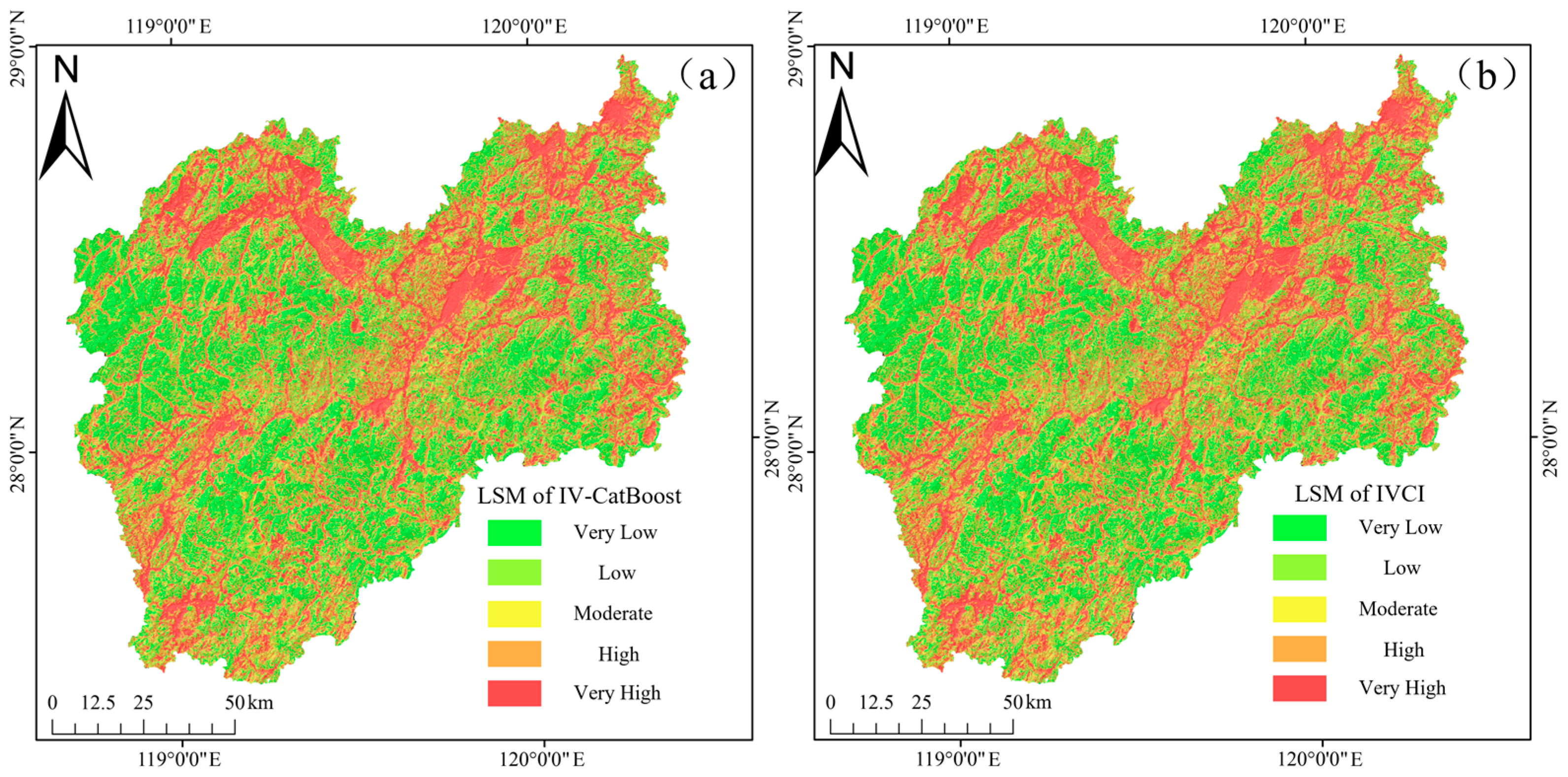
4.1.3. Landslide Susceptibility Mapping Using the IV-CatBoost Model

After successive model fitting iterations, the optimal learning rate was determined to be 0.091, with a max depth of nine, and a minibatch fraction of nine. This resulted in an RMSE of 0.24, an R² of 0.77, and an MAE of 0.16 for the top-performing model. All data from the study area were input into the trained model for landslide susceptibility prediction. The predicted values (ranging from 0 to 1) were obtained, and ArcGIS’s natural breaks method was used to divide them into five susceptibility levels: very high susceptibility (0.85 to 1.0), high susceptibility (0.6 to 0.85), moderate susceptibility (0.36 to 0.60), low susceptibility (0.13 to 0.36), and very low susceptibility (0 to 0.13). The results are shown in Figure 7.

According to

Table 3. Contingency matrix applied to the LSM considering the average velocity in each cell. (The subsidence results obtained from SBAS-InSAR were classified into five categories using the natural breaks method, where higher grades correspond to greater deformation rates).

Landslide Susceptibility Class	Rank	InSAR Deformation Rate Class
		1	2	3	4	5
VL	1	0	+1	+2	+3	+4
L	2	0	0	+1	+2	+3
M	3	0	0	0	+1	+2
H	4	0	0	0	0	+1
VH	5	0	0	0	0	0

, the area proportions of different susceptibility levels from very high to very low are 23.78%, 17.52%, 17.44%, 19.63%, and 21.63%, respectively. Through validation with existing landslide points, it was found that 90.71% of the existing landslide points fall within the high and very high susceptibility zones, while only 1.06% are located in the very low susceptibility zone. Using Python (3.10) with sklearn-learn (1.3.0), the model was evaluated using the 30% validation dataset, and the ROC curve was plotted. The ROC curve results are shown in Figure 8. The AUC value on this validation dataset is 0.88, indicating that the model’s predictions for new feature data are reasonably accurate and reliable.

The model’s predictions show that the high and very high susceptibility zones are concentrated in the range of elevation 542 m and slope 17°, mainly located within 0 to 300 m from both sides of the road, often found in cultivated areas. On the other hand, the low and very low susceptibility zones have a broader distribution, mainly located beyond 450 m from the road, often found in forested areas. These areas are generally at higher elevations, less affected by human activities, and in a stable susceptibility state.

4.2. SBAS-InSAR Results

The deformation rate in the Line of Sight (LOS) direction calculated by SBAS-InSAR technology is shown in Figure 9. The annual deformation rates in the study area range from −30.0 mm/y to 30.0 mm/y, where positive values indicate surface uplift and negative values represent surface subsidence. The average subsidence rate is 5.03 mm/y. Due to the hilly terrain and dense vegetation in the high-altitude regions in the study area, there were areas affected by decorrelation, leading to significant data gaps. The main subsidence areas are located in the western mountainous valleys and urban residential areas of the study area.

4.3. IVCI Model Results

Initially, we resampled the resolution of the SBAS-InSAR results to 30 m × 30 m, matching the grid size of the initial IV-CatBoost map. The results were then classified into five categories based on the natural breaks of annual deformation rates: <−14.88 mm/y, −14.88 mm/y to −9.14 mm/y, −9.14 mm/y to −5.39 mm/y, −5.39 mm/y to −2.46 mm/y, and >−2.46 mm/y. Each category was assigned a value of 5, 4, 3, 2, or 1. In order to ensure the accuracy of the model, no interpolation was performed in the blank areas. Only areas with annual subsidence rate results were refined. The data shown in Table 2 and landslide susceptibility were combined using ArcGIS to obtain the combined IVCI model. The updated results are shown in Figure 7.

The distribution of susceptibility zones in the IVCI model is similar to the IV-CatBoost zoning. The IVCI model results (

Table 4. IV-CatBoost model areas of the landslide susceptibility classes. Very-high susceptibility zones (VH); high susceptibility zones (H); moderate susceptibility zones (M); low susceptibility zones (L); very-low susceptibility zones (VL).

	Landslide Susceptibility Classes
	VH	H	M	L	VL
Area of zone (km2)	4102.33	3022.40	3009.27	3387.04	3732.14
Proportion (%)	23.78%	17.52%	17.44%	19.63%	21.63%
Landslide ratio (%)	74.16%	16.55%	6.02%	2.21%	1.06%

) show a reduction in the very low, low, and moderate susceptibility zones, while an increase is observed in the high and very high susceptibility zones. The differences in proportions between the zones are within 0.9%, indicating that the IV-CatBoost model’s classification trend is correct, although some regions require further refinement. To visually observe the changes in the grid before and after refinement, the grids were subtracted before and after integration to facilitate the analysis of changes in different susceptibility levels. According to

Table 5. Corrections of the partition differences before and after the model.

Landslide Susceptibility Class	IV-CatBoost		IVCI		Landslide Susceptibility Increase
Class	No. Cells	%	NO. Cells	%	Class	No. Cells
VL	4,146,823	21.63%	4,071,042	21.24%	0	19,005,155
L	3,763,380	19.63%	3,741,168	19.51%	+1	94,124
M	3,343,630	17.44%	3,372,395	17.59%	+2	46,992
H	3,358,220	17.52%	3,403,205	17.75%	+3	19,535
VH	4,558,886	23.78%	4,583,129	23.91%	+4	5133

, after integration, there were 94,124 grids (84.71 km²) that had their susceptibility levels increased by one level, 46,992 grids (42.29 km²) increased by two levels, 19,535 grids (17.58 km²) increased by three levels, and 5133 grids (4.62 km²) increased by four levels. In total, 165,784 grids obtained a more accurate susceptibility classification under the correction of InSAR.

In Figure 10, there are three distinct areas where the susceptibility levels have undergone significant corrections. To provide a clearer explanation of the model’s refinements and validate the accuracy of the IVCI model, these areas are labeled as Y-1, Y-2, and Y-3. Detailed discussions on these significant correction areas are presented in Section 5.1.

5. Discussion

5.1. IVCI Model Verification and Evaluation

To assess the accuracy of the model after integrating InSAR, this study selected three significant correction areas for the validation and evaluation of the IVCI model, using both SBAS-InSAR and optical remote sensing images.

The Y-1 region is situated at elevations ranging from 1070 to 1170 m, with most slopes falling within the 20° to 25° range. The character of the terrain in this region is more susceptible to landslide hazards (Figure 11). According to the interpretation of various optical images from different time periods, a shallow surface landslide developed near the toe of the slope close to the road in February 2011. In April 2017, eight shallow landslides occurred within this area, characterized by elongated shapes, with most of the landslide mass being soil (Figure 12). The optical remote sensing images indicated that the slope in this area is relatively unstable and prone to minor landslides.

The SBAS-InSAR results (Figure 13) indicate that the subsidence rate within the Y-1 area is mostly greater than 10 mm/y, suggesting ongoing slope subsidence deformation. To understand the variation of subsidence within the slope, representative point P-1 (E 176.230548°, N 15.189933°) was selected within Y-1, based on the interpretation results from optical remote sensing. Based on the settlement measurements of P-1 (Figure 13), the point remains in a fluctuating state, experiencing significant displacements after the rainy season each year, with a maximum displacement of 40 mm. Although some rebound phenomena are observed, the overall condition indicates settling.

The Y-2 area is located at elevations ranging from 860 to 960 m, with most slopes falling between 25° and 30°, making the terrain relatively steep (Figure 14). The roads in the area are more susceptible to the impact of landslides and other disasters. According to the interpretation of various optical images from different time periods, seven shallow landslides occurred near the sides of the roads, with some containing small rock fragments, in May 2012 (Figure 15). In October 2015, another shallow surface landslide occurred within the scope of landslide area (5). The interpretation results indicate that the slopes on both sides of the roads in this area are prone to small-scale shallow landslides under various disturbances.

The SBAS-InSAR results show (Figure 16) that the subsidence rate in the Y-2 area is mostly greater than 10 mm/y. Based on the settlement data at point P-2 (E 119.340640°, N 27.822157°) (Figure 16), it is clear that this point experiences fluctuations akin to P-1. Settlement is closely tied to the rainy season, with a maximum displacement of 60 mm. Although some rebound is observed, the overall trend is still downward.

The Y-3 area is situated at elevations ranging from 1100 to 1160 m, with the majority of slopes having gradients between 15° and 20° (Figure 17). While there is a significant difference in altitude, the slopes exhibit relatively minor variations in gradient. According to the interpretation of various optical images from different time periods, three shallow surface landslides were observed on the slopes in April 2013. In March 2016, another shallow surface landslide developed. The (5) and (6) slopes in this area, characterized by bare rock surfaces in different seasons, are susceptible to rockfall and similar disasters (Figure 18). These slopes are in an overall unstable situation.

The deformations in the Y-3 area are mostly between 15 mm/y and 20 mm/y (Figure 19). Based on the settlement measurements at point P-3 (E 119.280389°, N 27.604171°) (Figure 19), the area experienced a maximum settlement exceeding 45 mm, despite noticeable rebound phenomena in the later period. Overall, there is a clear indication of descent.

Based on the above findings, it is clear that the three distinct abnormal areas exhibit a pattern of subsidence deformation, and historical occurrences of landslide disasters are evident in each of these areas. This suggests that these three zones are in an unstable condition, making them susceptible to landslides. However, the IV-CatBoost model primarily classified these areas as having low to very low susceptibility, which does not align well with the current slope conditions. Upon adjustment using the IVCI model, the majority of grid cells within these zones were reclassified into the high and very high susceptibility categories, more accurately reflecting the real slope conditions. This underscores the superiority of the IVCI model over traditional approaches.

To comprehensively validate the precision of the IVCI model, an ROC curve was generated for the new model, and the outcomes are depicted in Figure 20. The AUC value for the IVCI model stands at 0.90, surpassing the IV-CatBoost model’s value of 0.88. This signifies that the IVCI model maintains a higher level of accuracy and precision on a substantial dataset compared to the IV-CatBoost model.

5.2. Feature Importance Analysis

To gain a comprehensive and accurate understanding of the model’s internal operations, we calculated the SHAP values of the model’s validation set [46,47]. The rankings of feature importance and SHAP values after interpreting the model are shown in Figure 21. From the results, we can see the significant impact of factors such as road distance, surface roughness, aspect, land use type, plane curvature, NDVI, and annual precipitation. Referring to Figure 5, it is evident that roughness and slope have higher impacts among terrain factors, with roughness carrying greater weight, while the other terrain factors have relatively lower impacts. On the other hand, factors like distance to rivers, profile curvature, lithology, distance to faults, and TWI have relatively smaller impacts on the model. These rankings of feature importance align with the interpretations from optical remote sensing and on-site observations. In this model, terrain factors and the influence of human activities have higher importance. Land use type and distribution factors have moderate importance, while meteorological hydrology and engineering geology factors have relatively lower importance in the model.

Given the minor impact of lower-ranked factors on the model, this study selectively examines the primary seven influential factors for analytical simplicity. As depicted in Figure 21, there exists a negative correlation between road proximity and the projected susceptibility to landslides, where closer proximity to roads corresponds to higher susceptibility, and increased distance results in lower susceptibility. As the study area lies within a hilly landscape in the central mountains, construction activities such as roads and tunnels are undertaken to enhance accessibility. However, these projects often involve slope cutting, internal excavation, and alteration of the original stress distribution within the bedrock. The presence of weak features like structural surfaces within slope rock formations could significantly compromise slope stability [48], thereby escalating the vulnerability to landslides and other geological hazards.

Elevation, roughness, and gradient factors share similarities with the terrain influence factor. Topographical attributes are prerequisites for the occurrence of landslide disasters [49]. As the slope gradient increases, the extent of the stress unloading zone on the slope surface widens, resulting in elevated concentrated stress at the slope toe, thus raising the probability of landslides. Steeper slopes experience higher internal stress within the slope mass, making them more prone to deformation and the formation of landslides. Referring to Figure 22, the patterns of slope and roughness demonstrate resemblance; higher predictive values primarily cluster within the 22° slope range, while roughness predominantly centers around 1.44, indicating frequent minor-scale landslides in the vicinity of residences. Land use classification mirrors the impact of human activities, with extensive human interventions observed in cultivated and anthropogenically altered land surfaces. In contrast, woodland and shrubland regions experience fewer human activities and thereby showcase relatively higher local stability.

5.3. Limitations of the Approach

Through model validation, incorporating dynamic deformation information to refine traditional machine learning models can improve the model and make the susceptibility zoning more accurate and precise, yielding results that better align with real-world conditions. However, this approach also has certain limitations. (a) InSAR technology is affected by terrain and vegetation conditions. In areas with steep terrain and dense vegetation, coherence loss may occur, leading to missing data in the study area. (b) Data sources can limit the acquisition of long-term data, preventing a comprehensive understanding of long-term slope deformation data in the research area. (c) The occurrence of landslide disasters in the study area is closely related to the rainy season and typhoons. However, the InSAR technology may not adequately reflect the subsidence changes before and after extreme rainfall events, thus failing to capture changes in susceptibility zoning following extreme rainfall. Therefore, the next phase of our research will introduce InSAR data before and after extreme weather events to enhance the applicability of the IVCI model in the area.

6. Conclusions

This study selected Lishui, southern China, as the study area, where landslides frequently occur due to factors such as human activities, terrain, and geological structures. Refining the susceptibility mapping research in this area is of great practical significance for disaster reduction and prevention.

(1)

This study employed multi-temporal optical remote sensing images and the IV method to refine the selection of landslide and non-landslide points within traditional machine learning models. This process effectively alleviated the dimensional influence among different features. Due to the removal of dimensionality differences, the data that are fed into the model for IV-based classification result from calculations. Compared to ensemble learning models such as LightGBM and XGBoost, CatBoost autonomously manages categorical features, reducing the complexity of feature preprocessing. Additionally, it is less susceptible to outliers and noise, ensuring a more stable and accurate model.

(2)

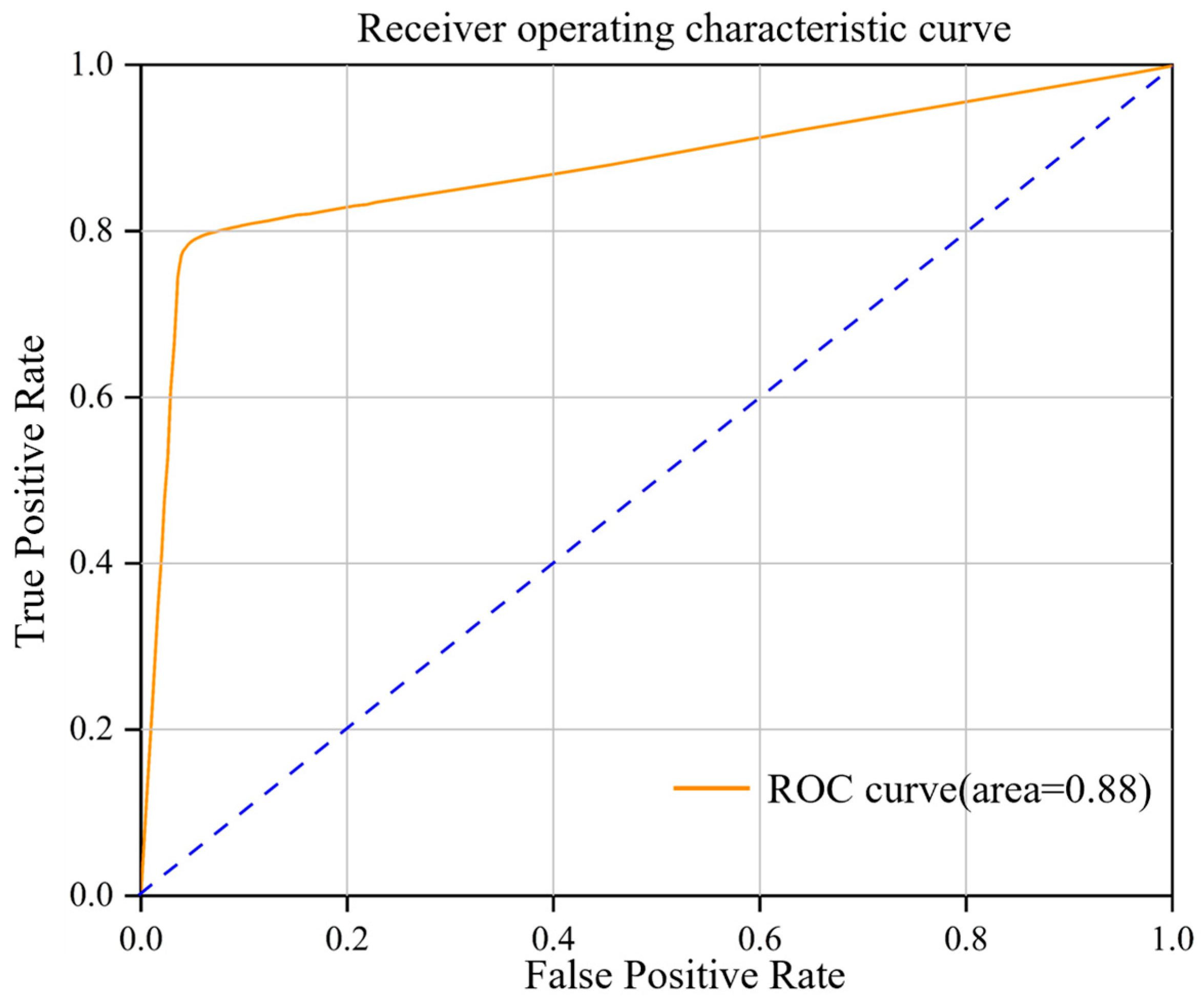
Using the hyperopt framework for hyperparameter optimization, we constructed the IV-CatBoost model, achieving an RMSE of 0.24, an R² of 0.77, and an MAE of 0.16, demonstrating a high level of accuracy. In the resulting model, 90.71% of landslide points are located within the VH and H regions, with only 1.06% falling within the VL region, resulting in an AUC value of 0.88.

(3)

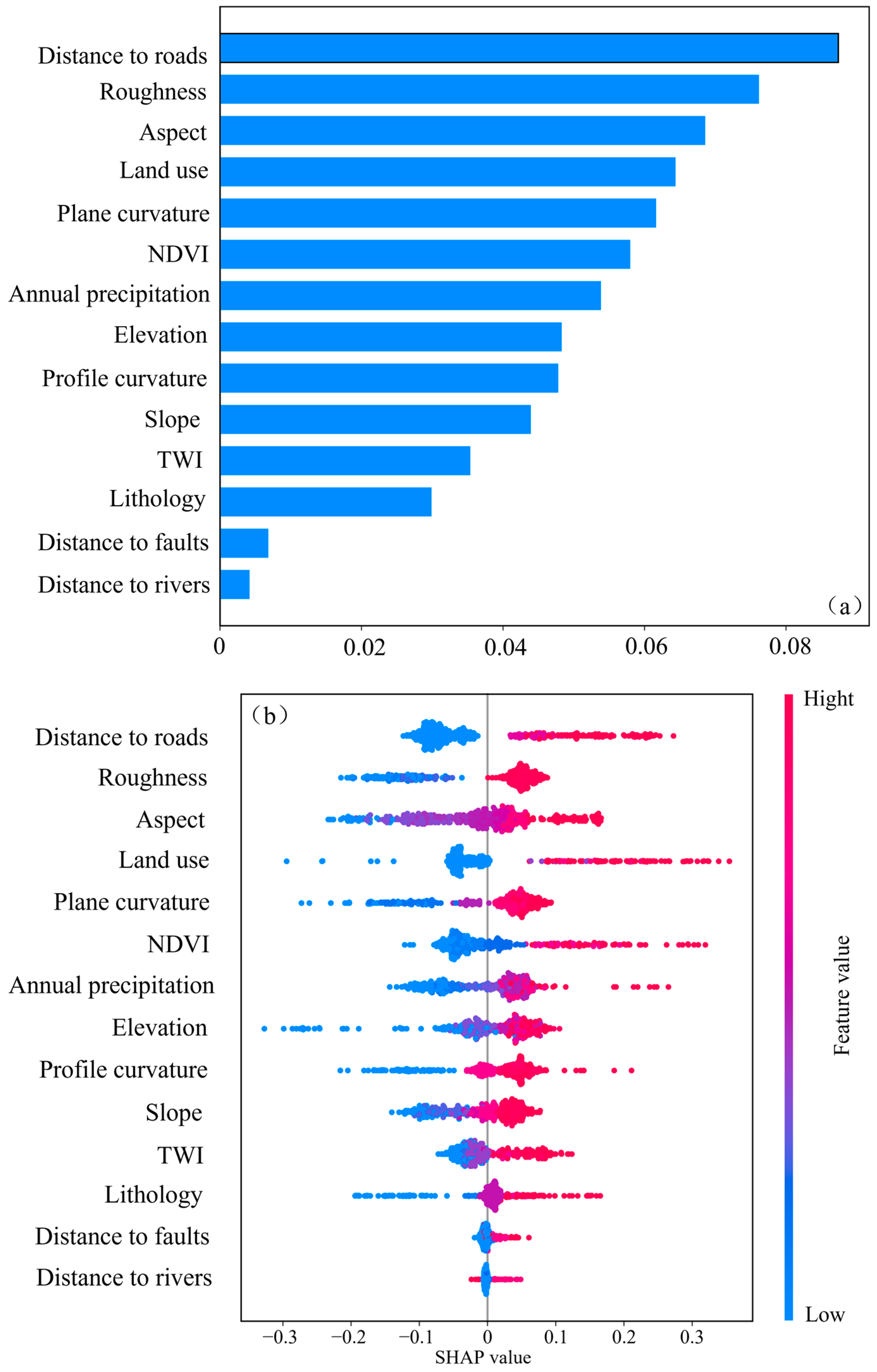
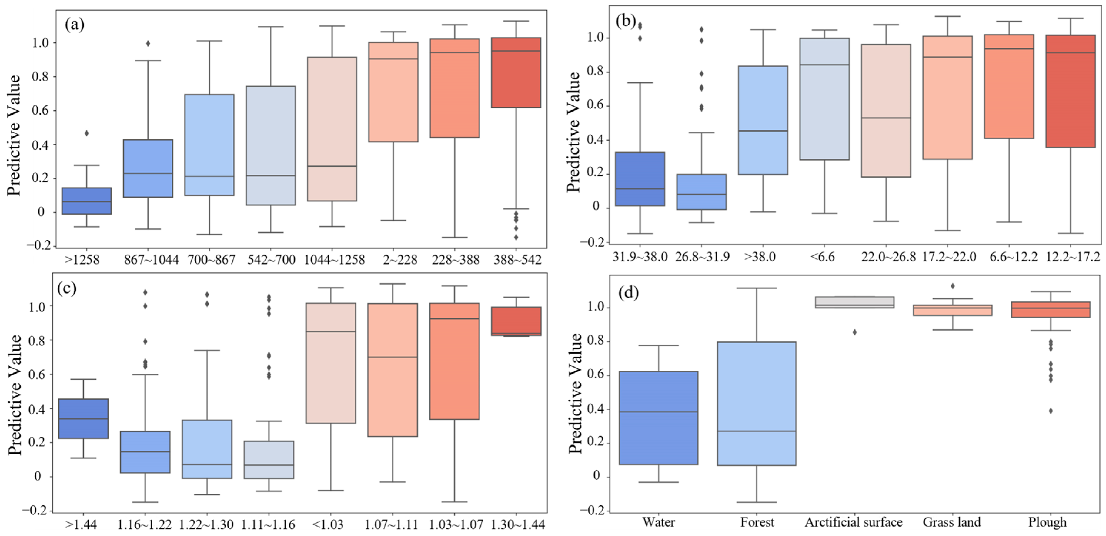
To make the model interpretable, SHAP values were computed for the features, revealing the ranking of feature importance and their distributions. The results showed that the distance to roads and terrain factors have relatively significant impacts on the model, aligning with optical remote sensing interpretation results and on-site conditions, thus reflecting the model’s accuracy.

(4)

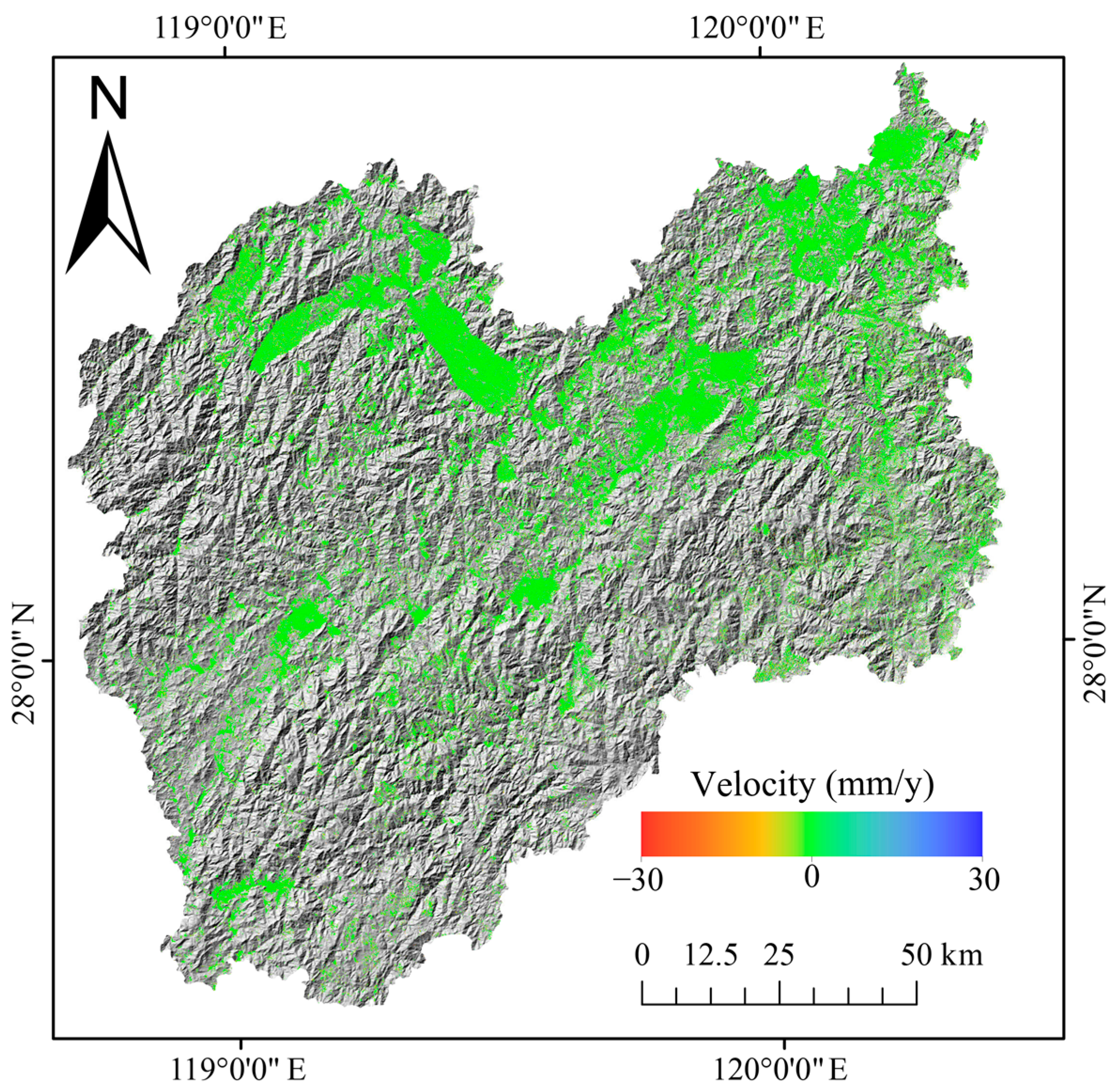
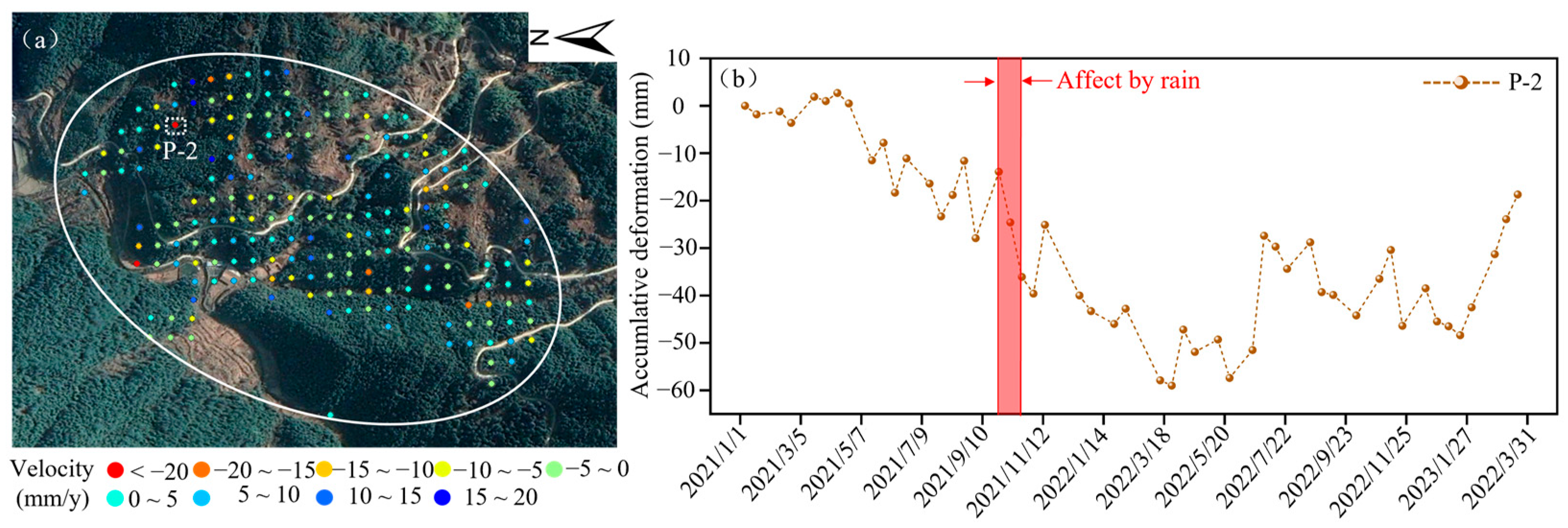
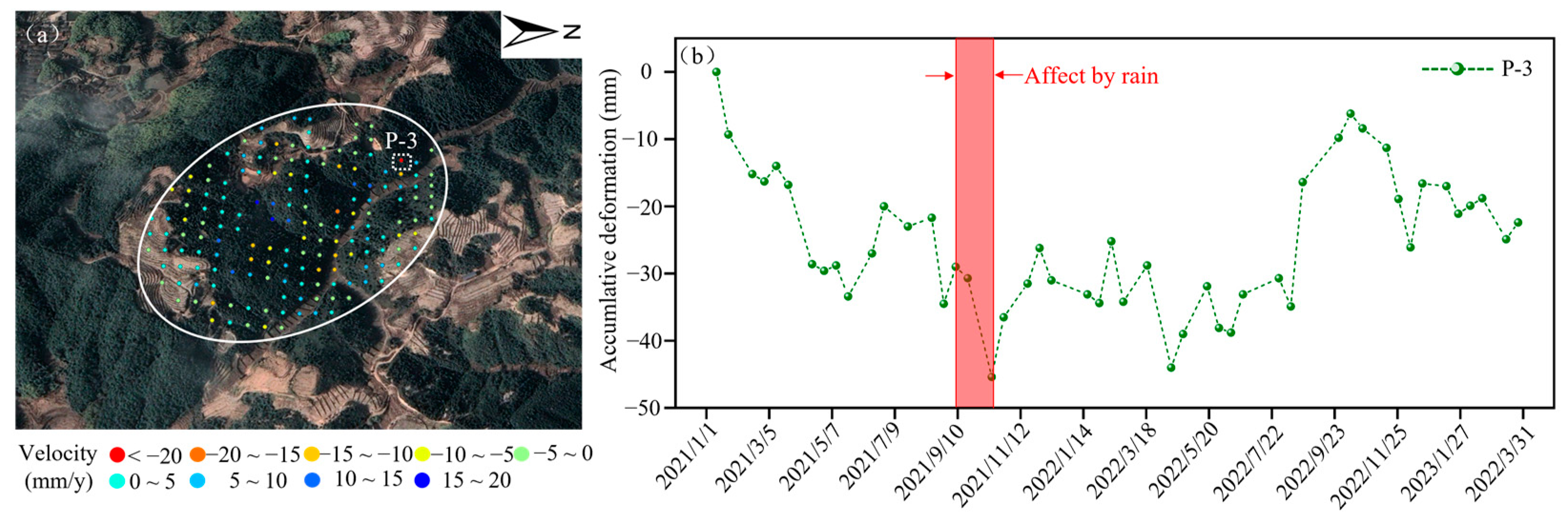
This study requires obtaining long-term surface deformation information in the research area to precisely understand the slope conditions. Therefore, DInSAR has limitations, and it is recommended to choose PS-InSAR and SBAS-InSAR, which can capture extended temporal sequences. Given that the research area is hilly, with most regions being mountainous, to ensure accurate computation results, we selected the SBAS-InSAR method for this InSAR calculation to acquire precise surface deformation information in the research area. The SBAS-InSAR results indicate that the majority of the regions exhibit annual deformation between −10.0 mm/y and 10.0 mm/y.

(5)

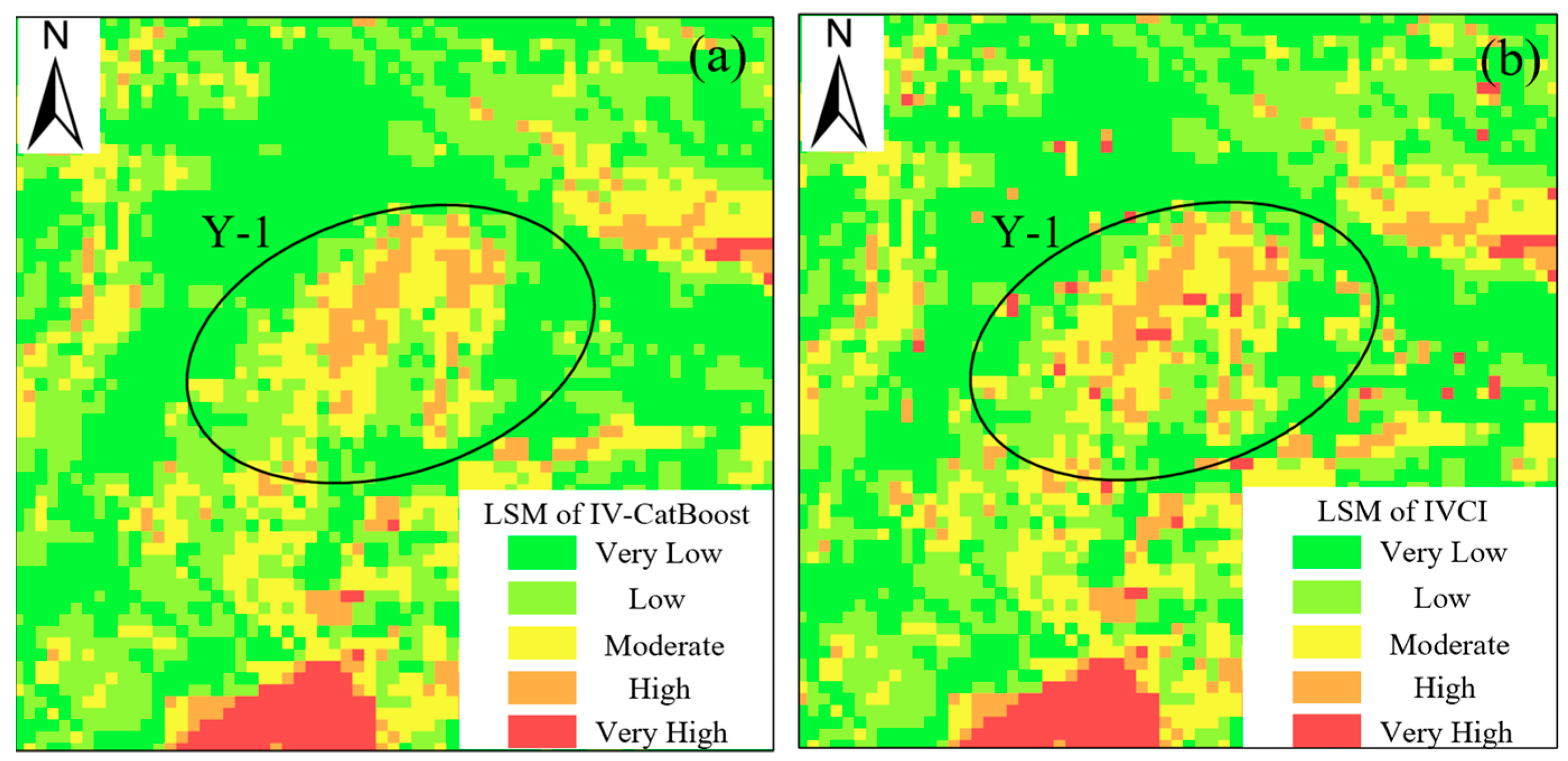
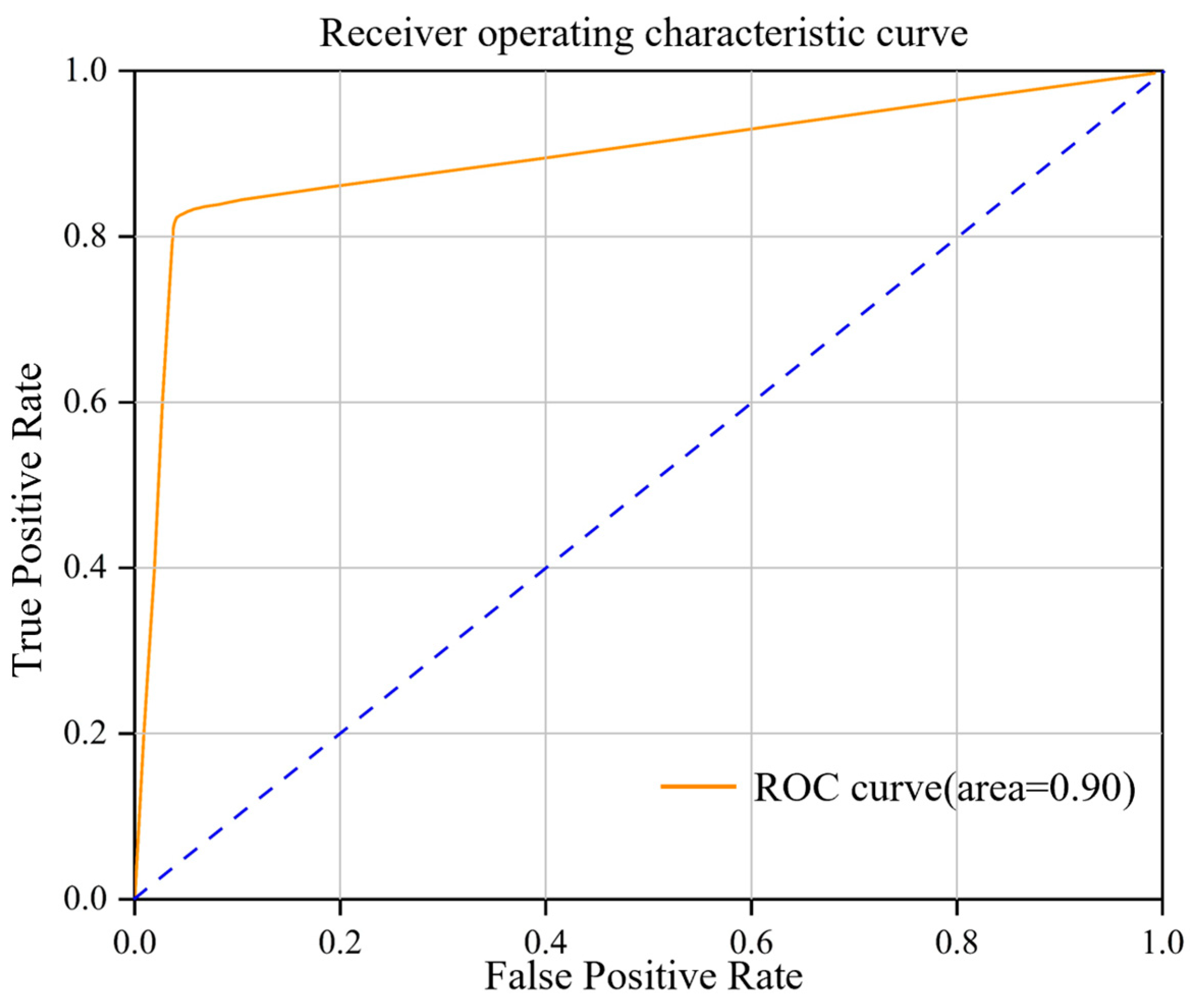
By integrating SBAS-InSAR technology, the existing IV-CatBoost model was augmented with dynamic deformation factors to establish the IVCI model. As a result, 165,784 grids attained enhanced susceptibility classification precision through InSAR-driven refinements, yielding an AUC value of 0.90. Quantitatively, the IVCI model’s accuracy surpasses that of the IV-CatBoost model.

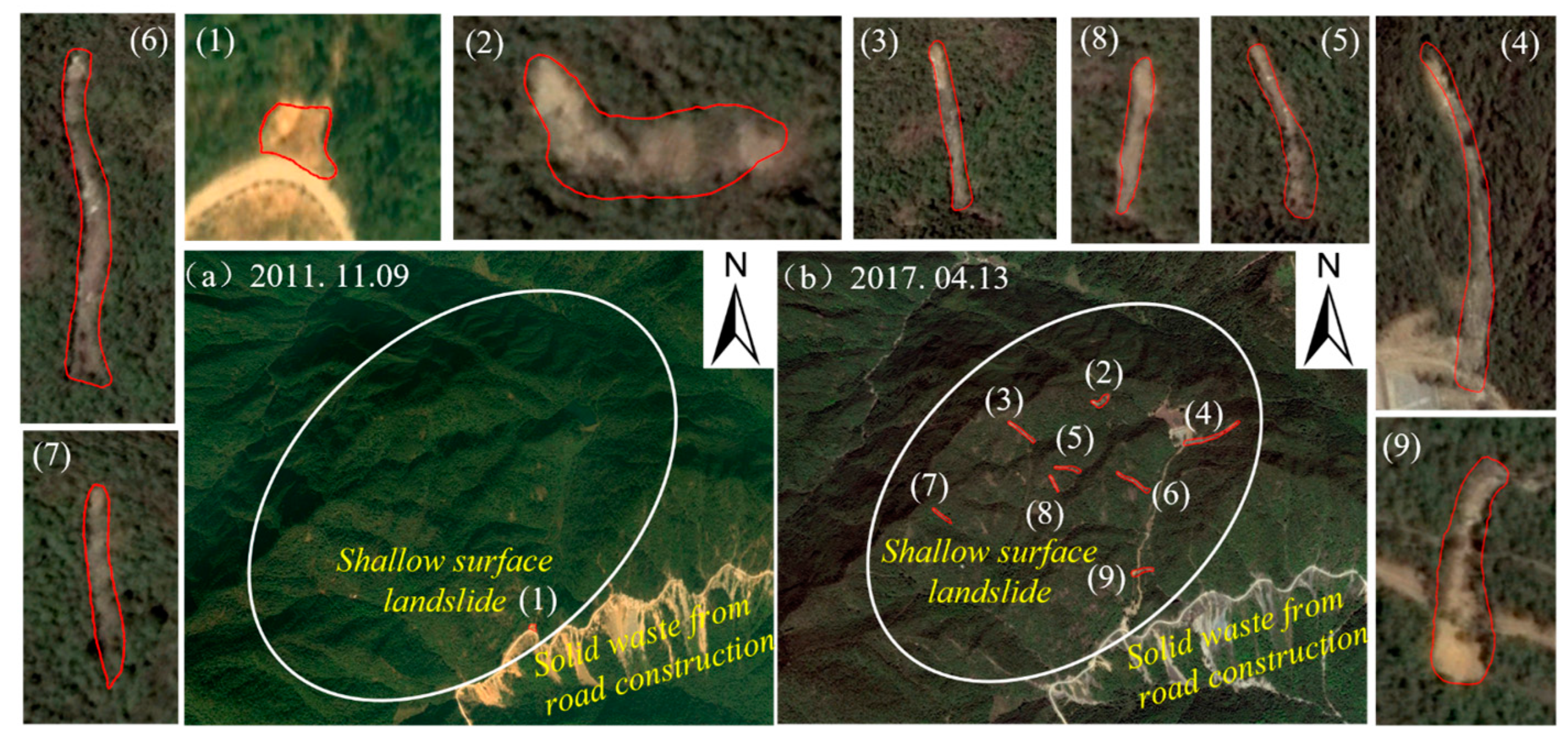
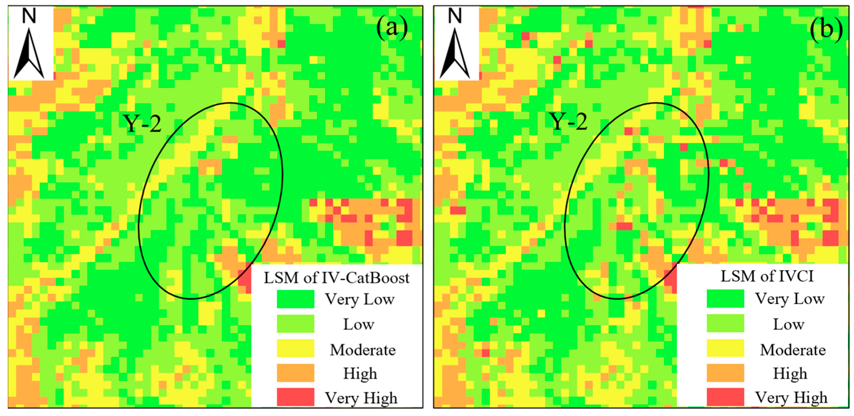
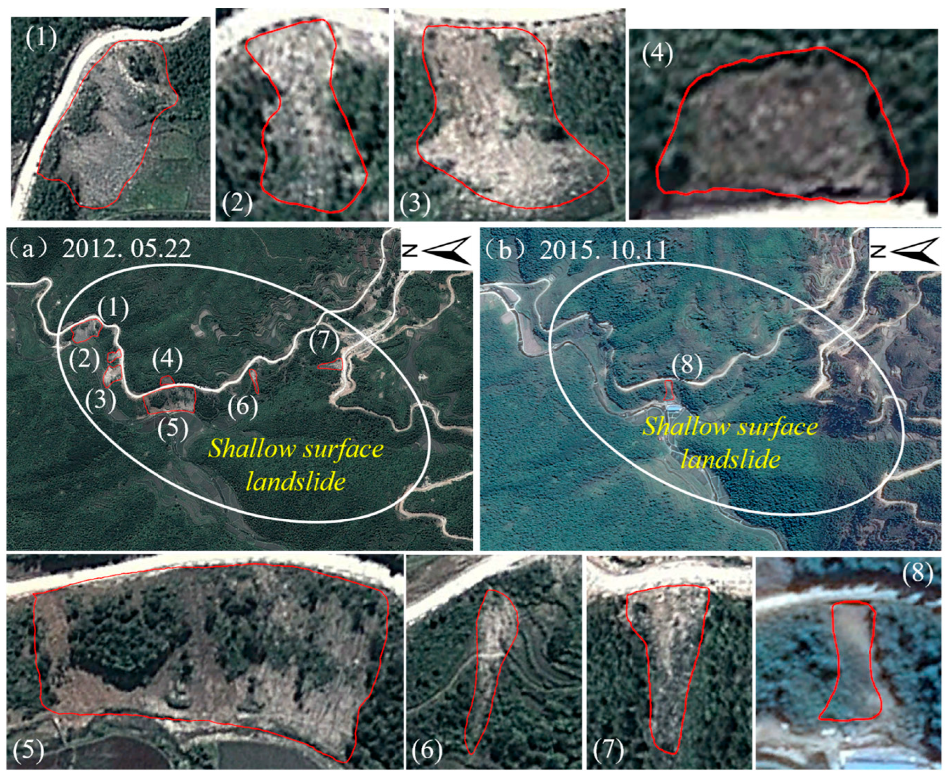
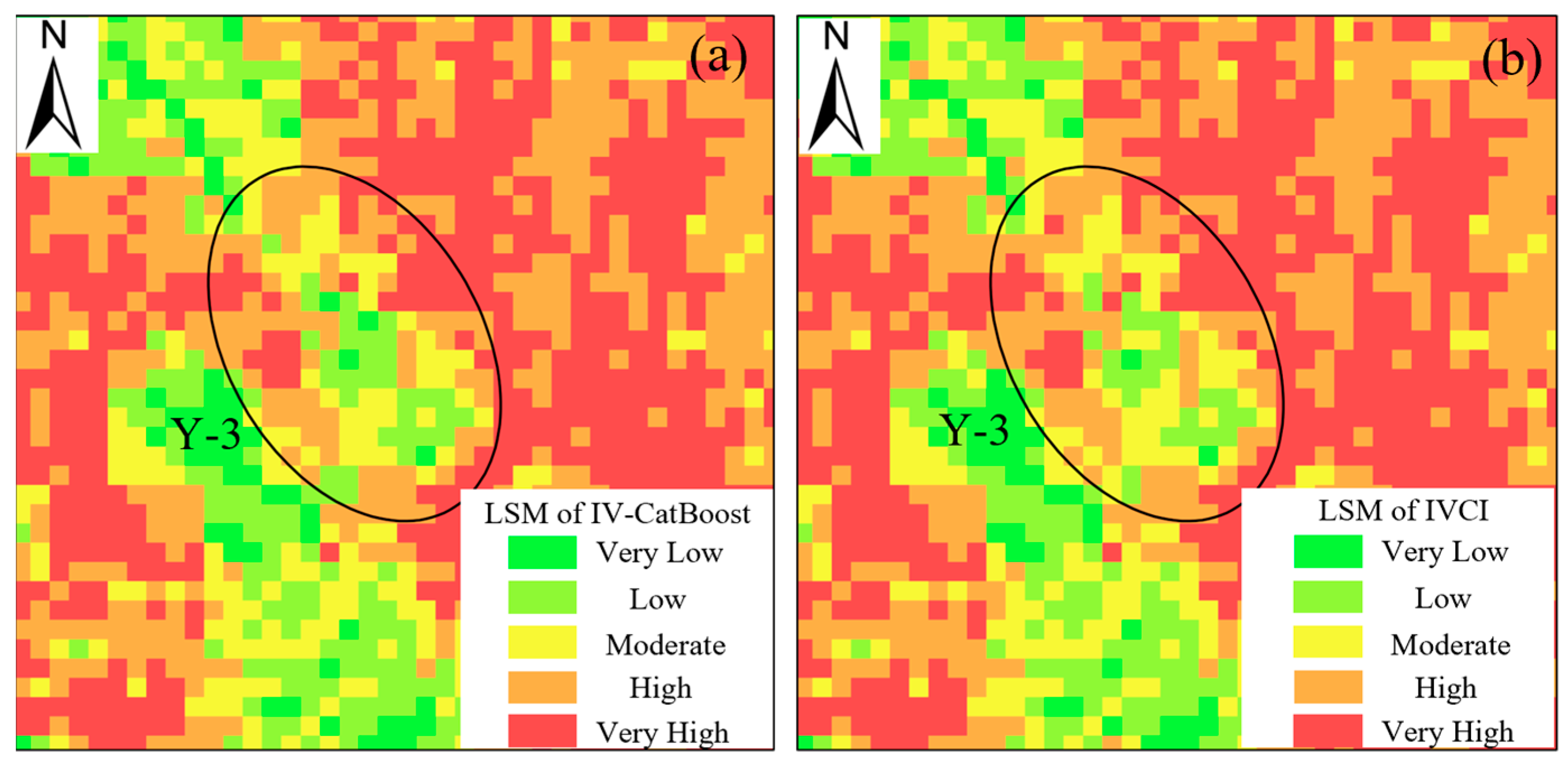
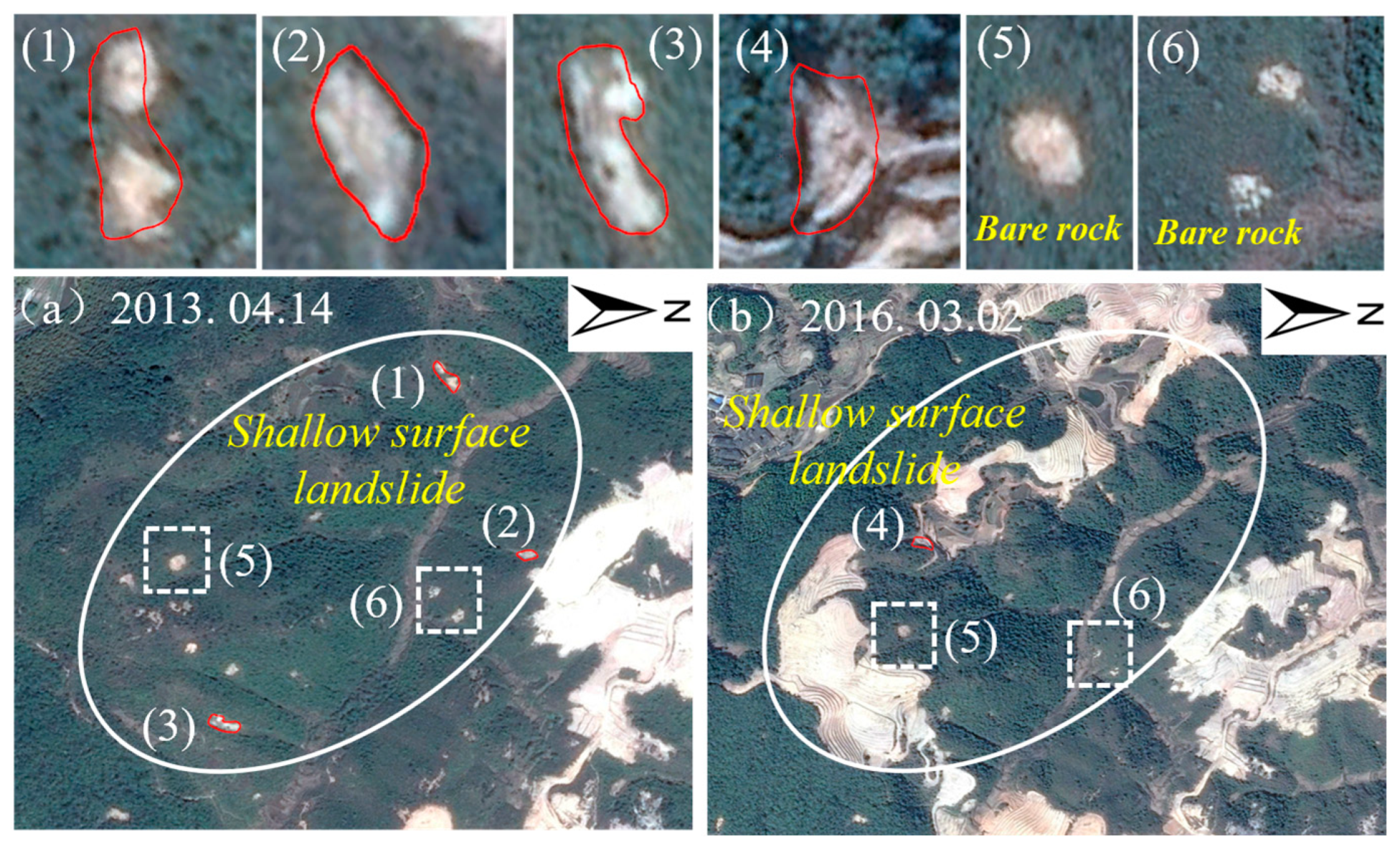
(6)

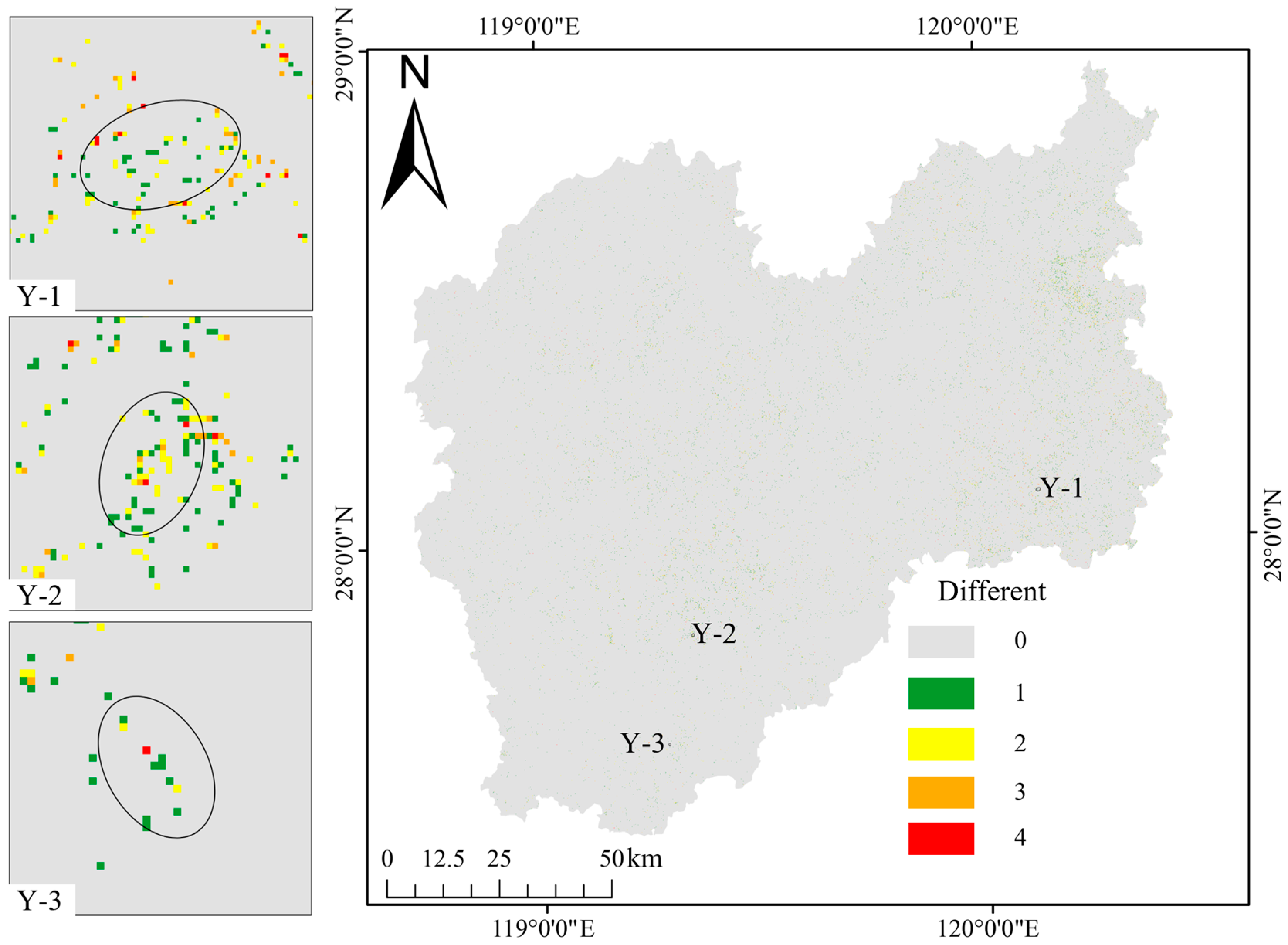
By analyzing the differences between the IV-CatBoost model and the IVCI model, three areas with significant modifications were identified. Validation using optical remote sensing images and SBAS-InSAR results confirmed that these areas are in an unstable state, and the results of the IV-CatBoost model did not align with the ground truth, leading to misclassifications. This illustrates that the introduction of InSAR technology can effectively identify and correct classification errors in the model, further enhancing the accuracy of the susceptibility model.

In conclusion, the IVCI model established based on the judgment matrix can refine traditional susceptibility mapping, making susceptibility zoning more accurate and providing valuable references and data support for local disaster reduction, prevention, and engineering projects.

References

1. Brabb, E.E. Innovative approaches to landslide hazard and risk mapping. In Proceedings of the International Landslide Symposium Proceedings, Toronto, ON, Canada, 23–31 August 1985. [Google Scholar]
2. Pei, Y.Q.; Qiu, H.J.; Yang, D.D.; Liu, Z.J.; Ma, S.Y.; Li, J.Y.; Cao, M.M.; Wufuer, W. Increasing landslide activity in the Taxkorgan River Basin (eastern Pamirs Plateau, China) driven by climate change. Catena 2023, 223, 106911. [Google Scholar] [CrossRef]
3. Zhan, J.W.; Yu, Z.Y.; Lv, Y.; Peng, J.B.; Song, S.Y.; Yao, Z.W. Rockfall Hazard Assessment in the Taihang Grand Canyon Scenic Area Integrating Regional-Scale Identification of Potential Rockfall Sources. Remote Sens. 2022, 14, 3021. [Google Scholar] [CrossRef]
4. Jiang, S.H.; Huang, J.S.; Huang, F.M.; Yang, J.H.; Yao, C.; Zhou, C.B. Modelling of spatial variability of soil undrained shear strength by conditional random fields for slope reliability analysis. Appl. Math. Model. 2018, 63, 374–389. [Google Scholar] [CrossRef]
5. Kavoura, K.; Sabatakakis, N. Investigating landslide susceptibility procedures in Greece. Landslides 2019, 17, 127–145. [Google Scholar] [CrossRef]
6. Marjanović, M.; Kovačević, M.; Bajat, B.; Voženílek, V. Landslide susceptibility assessment using SVM machine learning algorithm. Eng. Geol. 2011, 123, 225–234. [Google Scholar] [CrossRef]
7. Thomas, A.V.; Saha, S.; Danumah, J.H.; Raveendran, S.; Prasad, M.K.; Ajin, R.S.; Kuriakose, S.L. Landslide Susceptibility Zonation of Idukki District Using GIS in the Aftermath of 2018 Kerala Floods and Landslides: A Comparison of AHP and Frequency Ratio Methods. J. Geovis. Spat. Anal. 2021, 5, 21. [Google Scholar] [CrossRef]
8. Khosravi, K.; Nohani, E.; Maroufinia, E.; Pourghasemi, H.R. A GIS-based flood susceptibility assessment and its mapping in Iran: A comparison between frequency ratio and weights-of-evidence bivariate statistical models with multi-criteria decision-making technique. Nat. Hazards 2016, 83, 947–987. [Google Scholar] [CrossRef]
9. Shahabi, H.; Hashim, M.; Ahmad, B.B. Remote sensing and GIS-based landslide susceptibility mapping using frequency ratio, logistic regression, and fuzzy logic methods at the central Zab basin, Iran. Environ. Earth Sci. 2015, 73, 8647–8668. [Google Scholar] [CrossRef]
10. Yalcin, A.; Reis, S.; Aydinoglu, A.C.; Yomralioglu, T. A GIS-based comparative study of frequency ratio, analytical hierarchy process, bivariate statistics and logistics regression methods for landslide susceptibility mapping in Trabzon, NE Turkey. Catena 2011, 85, 274–287. [Google Scholar] [CrossRef]
11. Tehrany, M.S.; Pradhan, B.; Jebur, M.N. Spatial prediction of flood susceptible areas using rule based decision tree (DT) and a novel ensemble bivariate and multivariate statistical models in GIS. J. Hydrol. 2013, 504, 69–79. [Google Scholar] [CrossRef]
12. Hong, H.Y.; Tsangaratos, P.; Ilia, I.; Liu, J.Z.; Zhu, A.X.; Chen, W. Application of fuzzy weight of evidence and data mining techniques in construction of flood susceptibility map of Poyang County, China. Sci. Total Environ. 2018, 625, 575–588. [Google Scholar] [CrossRef] [PubMed]
13. Akinci, H.; Yavuz Ozalp, A. Landslide susceptibility mapping and hazard assessment in Artvin (Turkey) using frequency ratio and modified information value model. Acta Geophys. 2021, 69, 725–745. [Google Scholar] [CrossRef]
14. Deng, H.; Wu, X.; Zhang, W.; Liu, Y.; Li, W.; Li, X.; Zhou, P.; Zhuo, W. Slope-Unit Scale Landslide Susceptibility Mapping Based on the Random Forest Model in Deep Valley Areas. Remote Sens. 2022, 14, 4245. [Google Scholar] [CrossRef]
15. Towfiqul Islam, A.R.M.; Talukdar, S.; Mahato, S.; Kundu, S.; Eibek, K.U.; Pham, Q.B.; Kuriqi, A.; Linh, N.T.T. Flood susceptibility modelling using advanced ensemble machine learning models. Geosci. Front. 2021, 12, 101075. [Google Scholar] [CrossRef]
16. Huang, F.; Yin, K.; Huang, J.; Gui, L.; Wang, P. Landslide susceptibility mapping based on self-organizing-map network and extreme learning machine. Eng. Geol. 2017, 223, 11–22. [Google Scholar] [CrossRef]
17. Chen, W.; Pourghasemi, H.R.; Kornejady, A.; Zhang, N. Landslide spatial modeling: Introducing new ensembles of ANN, MaxEnt, and SVM machine learning techniques. Geoderma 2017, 305, 314–327. [Google Scholar] [CrossRef]
18. Thi Ngo, P.T.; Panahi, M.; Khosravi, K.; Ghorbanzadeh, O.; Kariminejad, N.; Cerda, A.; Lee, S. Evaluation of deep learning algorithms for national scale landslide susceptibility mapping of Iran. Geosci. Front. 2021, 12, 505–519. [Google Scholar] [CrossRef]
19. Wang, H.J.; Zhang, L.M.; Luo, H.Y.; He, J.; Cheung, R.W.M. AI-powered landslide susceptibility assessment in Hong Kong. Eng. Geol. 2021, 288, 106103. [Google Scholar] [CrossRef]
20. Habumugisha, J.M.; Chen, N.S.; Rahman, M.; Islam, M.M.; Ahmad, H.; Elbeltagi, A.; Sharma, G.; Liza, S.N.; Dewan, A. Landslide Susceptibility Mapping with Deep Learning Algorithms. Sustainability 2022, 14, 1734. [Google Scholar] [CrossRef]
21. Huang, W.B.; Ding, M.T.; Li, Z.H.; Yu, J.C.; Ge, D.Q.; Liu, Q.; Yang, J. Landslide susceptibility mapping and dynamic response along the Sichuan-Tibet transportation corridor using deep learning algorithms. Catena 2023, 222, 106866. [Google Scholar] [CrossRef]
22. Lv, L.; Chen, T.; Dou, J.; Plaza, A. A hybrid ensemble-based deep-learning framework for landslide susceptibility mapping. Int. J. Appl. Earth Obs. 2022, 108, 102713. [Google Scholar] [CrossRef]
23. Wang, Y.; Fang, Z.C.; Hong, H.Y. Comparison of convolutional neural networks for landslide susceptibility mapping in Yanshan County, China. Sci. Total Environ. 2019, 666, 975–993. [Google Scholar] [CrossRef] [PubMed]
24. Habibi, A.; Delavar, M.R.; Sadeghian, M.S.; Nazari, B.; Pirasteh, S. A hybrid of ensemble machine learning models with RFE and Boruta wrapper-based algorithms for flash flood susceptibility assessment. Int. J. Appl. Earth Obs. 2023, 122, 103401. [Google Scholar] [CrossRef]
25. Sahin, E.K. Implementation of free and open-source semi-automatic feature engineering tool in landslide susceptibility mapping using the machine-learning algorithms RF, SVM, and XGBoost. Stoch. Environ. Res. Risk Assess. 2023, 37, 1067–1092. [Google Scholar] [CrossRef]
26. Zhang, H.; Song, Y.; Xu, S.; He, Y.; Li, Z.; Yu, X.; Liang, Y.; Wu, W.; Wang, Y. Combining a class-weighted algorithm and machine learning models in landslide susceptibility mapping: A case study of Wanzhou section of the Three Gorges Reservoir, China. Comput. Geosci. 2022, 158, 104966. [Google Scholar] [CrossRef]
27. Pradhan, B.; Dikshit, A.; Lee, S.; Kim, H. An explainable AI (XAI) model for landslide susceptibility modeling. Appl. Soft Comput. 2023, 142, 110324. [Google Scholar] [CrossRef]
28. Iban, M.C.; Bilgilioglu, S.S. Snow avalanche susceptibility mapping using novel tree-based machine learning algorithms (XGBoost, NGBoost, and LightGBM) with eXplainable Artificial Intelligence (XAI) approach. Stoch. Environ. Res. Risk Assess. 2023, 37, 2243–2270. [Google Scholar] [CrossRef]
29. Meghanadh, D.; Kumar Maurya, V.; Tiwari, A.; Dwivedi, R. A multi-criteria landslide susceptibility mapping using deep multi-layer perceptron network: A case study of Srinagar-Rudraprayag region (India). Adv. Space Res. 2022, 69, 1883–1893. [Google Scholar] [CrossRef]
30. Li, G.; Ding, Z.g.; Li, M.f.; Hu, Z.h.; Jia, X.t.; Li, H.; Zeng, T. Bayesian Estimation of Land Deformation Combining Persistent and Distributed Scatterers. Remote Sens. 2022, 14, 3471. [Google Scholar] [CrossRef]
31. Amoroso, N.; Cilli, R.; Nitti, D.O.; Nutricato, R.; Iban, M.C.; Maggipinto, T.; Tangaro, S.; Monaco, A.; Bellotti, R. PSI Spatially Constrained Clustering: The Sibari and Metaponto Coastal Plains. Remote Sens. 2023, 15, 2560. [Google Scholar] [CrossRef]
32. Chen, J.; Liu, L.; Zhang, T.j.; Cao, B.; Lin, H. Using Persistent Scatterer Interferometry to Map and Quantify Permafrost Thaw Subsidence: A Case Study of Eboling Mountain on the Qinghai-Tibet Plateau. J. Geophys. Res. Earth Surf. 2018, 123, 2663–2676. [Google Scholar] [CrossRef]
33. Zhang, H.; Zeng, R.; Zhang, Y.; Zhao, S.; Meng, X.; Li, Y.; Liu, W.; Meng, X.; Yang, Y. Subsidence monitoring and influencing factor analysis of mountain excavation and valley infilling on the Chinese Loess Plateau: A case study of Yan’an New District. Eng. Geol. 2022, 297, 106482. [Google Scholar] [CrossRef]
34. Ciampalini, A.; Raspini, F.; Lagomarsino, D.; Catani, F.; Casagli, N. Landslide susceptibility map refinement using PSInSAR data. Remote Sens. Environ. 2016, 184, 302–315. [Google Scholar] [CrossRef]
35. Shen, C.Y.; Feng, Z.K.; Xie, C.; Fang, H.R.; Zhao, B.B.; Ou, W.H.; Zhu, Y.; Wang, K.; Li, H.W.; Bai, H.L.; et al. Refinement of Landslide Susceptibility Map Using Persistent Scatterer Interferometry in Areas of Intense Mining Activities in the Karst Region of Southwest China. Remote Sens. 2019, 11, 2821. [Google Scholar] [CrossRef]
36. Zhang, G.; Wang, S.Y.; Chen, Z.W.; Liu, Y.T.; Xu, Z.X.; Zhao, R.S. Landslide susceptibility evaluation integrating weight of evidence model and InSAR results, west of Hubei Province, China. Egypt. J. Remote Sens. 2023, 26, 95–106. [Google Scholar] [CrossRef]
37. Cao, C.; Zhu, K.X.; Xu, P.H.; Shan, B.; Yang, G.; Song, S.Y. Refined landslide susceptibility analysis based on InSAR technology and UAV multi-source data. J. Clean. Prod. 2022, 368, 133146. [Google Scholar] [CrossRef]
38. Wang, Y.M.; Wu, X.L.; Chen, Z.J.; Ren, F.; Feng, L.W.; Du, Q.Y. Optimizing the Predictive Ability of Machine Learning Methods for Landslide Susceptibility Mapping Using SMOTE for Lishui City in Zhejiang Province, China. Int. J. Environ. Res. Public Health 2019, 16, 368. [Google Scholar] [CrossRef]
39. Wu, Y.L.; Ke, Y.T.; Chen, Z.; Liang, S.Y.; Zhao, H.L.; Hong, H.Y. Application of alternating decision tree with AdaBoost and bagging ensembles for landslide susceptibility mapping. Catena 2020, 187, 104396. [Google Scholar] [CrossRef]
40. Huang, F.M.; Cao, Z.S.; Guo, J.F.; Jiang, S.H.; Li, S.; Guo, Z.Z. Comparisons of heuristic, general statistical and machine learning models for landslide susceptibility prediction and mapping. Catena 2020, 191, 104580. [Google Scholar] [CrossRef]
41. Dorogush, A.V.; Gulin, A.; Gusev, G.; Kazeev, N.; Ostroumova, L.; Vorobev, A. Fighting biases with dynamic boosting. arXiv 2017, arXiv:1706.09516. [Google Scholar]
42. Wasowski, J.; Bovenga, F. Investigating landslides and unstable slopes with satellite Multi Temporal Interferometry: Current issues and future perspectives. Eng. Geol. 2014, 174, 103–138. [Google Scholar] [CrossRef]
43. Zhao, R.; Li, Z.w.; Feng, G.c.; Wang, Q.j.; Hu, J. Monitoring surface deformation over permafrost with an improved SBAS-InSAR algorithm: With emphasis on climatic factors modeling. Remote Sens. Environ. 2016, 184, 276–287. [Google Scholar] [CrossRef]
44. Zhu, Z.; Gan, S.; Yuan, X.; Zhang, J. Landslide Susceptibility Mapping with Integrated SBAS-InSAR Technique: A Case Study of Dongchuan District, Yunnan (China). Sensors 2022, 22, 5587. [Google Scholar] [CrossRef] [PubMed]
45. Cantarino, I.; Carrion, M.A.; Goerlich, F.; Martinez Ibañez, V. A ROC analysis-based classification method for landslide susceptibility maps. Landslides 2019, 16, 265–282. [Google Scholar] [CrossRef]
46. Ekmekcioğlu, Ö.; Koc, K. Explainable step-wise binary classification for the susceptibility assessment of geo-hydrological hazards. Catena 2022, 216, 106379. [Google Scholar] [CrossRef]
47. Zhang, J.Y.; Ma, X.L.; Zhang, J.L.; Sun, D.L.; Zhou, X.Z.; Mi, C.L.; Wen, H.J. Insights into geospatial heterogeneity of landslide susceptibility based on the SHAP-XGBoost model. J. Environ. Manag. 2023, 332, 117357. [Google Scholar] [CrossRef]
48. Pradhan, S.P.; Siddique, T. Stability assessment of landslide-prone road cut rock slopes in Himalayan terrain: A finite element method based approach. J. Rock. Mech. Geotech. 2020, 12, 59–73. [Google Scholar] [CrossRef]
49. Rosi, A.; Tofani, V.; Tanteri, L.; Tacconi Stefanelli, C.; Agostini, A.; Catani, F.; Casagli, N. The new landslide inventory of Tuscany (Italy) updated with PS-InSAR: Geomorphological features and landslide distribution. Landslides 2018, 15, 5–19. [Google Scholar] [CrossRef]
Figure 1. Map of the study area and the distribution of landslide points. (a) The geographical location of the study area; (b) Elevation map of the city of Lishui with landslide locations.
Applsci 13 12817 g001
Figure 2. Optical remote sensing interpretation results of landslides in the city of Lishui using Google Earth imagery.
Applsci 13 12817 g002
Figure 3. Research workflow diagram.
Applsci 13 12817 g003
Figure 4. Temporal and spatial baselines of the SAR datasets employed in this study. (a) Time–position plot illustrating InSAR image acquisitions; (b) Time–baseline plot depicting interference pairs of SAR images.
Applsci 13 12817 g004
Figure 5. Impact factor correlation heat map (PlaneC: plane curvature; ProfC: profile curvature; Rough: roughness; Litho: lithology; LandU: land use; DTF: distance to faults; DRI: distance to rivers; DTR: distance to roads; AnnualP: annual precipitation).
Applsci 13 12817 g005
Figure 6. Landslide susceptibility map of IV: regions with very low and low susceptibility, and the distribution of non-landslide points.
Applsci 13 12817 g006
Figure 7. Landslide susceptibility maps of the (a) IV-CatBoost and (b) IVCI models.
Applsci 13 12817 g007
Figure 8. IV-CatBoost model ROC curve. An AUC value ranging from 0.7 to 0.9 indicates favorable model performance, signifying its heightened classification capability.
Applsci 13 12817 g008
Figure 9. Map of SBAS-InSAR annual subsidence rates.
Applsci 13 12817 g009
Figure 10. Map of the post-correction level differences between the IV-CatBoost and IVCI model.
Applsci 13 12817 g010
Figure 11. Comparison of landslide susceptibility for Y-1 under the (a) IV-CatBoost model and (b) IVCI model.
Applsci 13 12817 g011
Figure 12. Y-1 optical remote sensing interpretation. (1~9), delineated by the red lines, are all classified as shallow surface landslides. The images (a,b) are both derived from Maxar satellite data.
Applsci 13 12817 g012
Figure 13. The SBAS-InSAR results within Y-1. (a) Velocity map of the Y-1 SBAS-InSAR results; (b) map of P-1 cumulative settlement.
Applsci 13 12817 g013
Figure 14. Comparison of landslide susceptibility for Y-2 under the (a) IV-CatBoost model and (b) IVCI model.
Applsci 13 12817 g014
Figure 15. Y-2 optical remote sensing interpretation. (1~8), delineated by the red lines, are all classified as shallow surface landslides. (a) image from Maxar Technologies, (b) image from CNES/Airbus.
Applsci 13 12817 g015
Figure 16. The SBAS-InSAR results within Y-2. (a) Velocity map of the Y-2 SBAS-InSAR results; (b) map of P-2 cumulative settlement.
Applsci 13 12817 g016
Figure 17. Comparison of landslide susceptibility for Y-3 under the (a) IV-CatBoost model and (b) IVCI model.
Applsci 13 12817 g017
Figure 18. Y-3 optical remote sensing interpretation. (1~4), delineated by the red lines, are all classified as shallow surface landslides. Both (5) and (6) are characterized as bare rock. Images (a,b) are both derived from CNES/Airbus satellite data.
Applsci 13 12817 g018
Figure 19. The SBAS-InSAR results within Y-3. (a) Velocity map of the Y-3 SBAS-InSAR results; (b) map of P-3 cumulative settlement.
Applsci 13 12817 g019
Figure 20. IVCI model ROC curve. An AUC value exceeding 0.9 signifies exceptional model performance, demonstrating outstanding classification capability within the model.
Applsci 13 12817 g020
Figure 21. Map of the results of the feature importance analysis. (a) Feature importance ranking; (b) SHAP summary plot of the test dataset.
Applsci 13 12817 g021
Figure 22. Distribution of predicted values across (a) elevation, (b) slope, (c) roughness, and (d) land use.
Applsci 13 12817 g022