Abstract
This article presents the basic principles for an Extremely Low Frequency (ELF) IoT-based isotropic meter implementation, which can measure magnetic flux density from 100 nT up to 10 μT. The identical sensor probes are used for isotropic field measurements in the X, Y, and Z planes. The prototype has a flat response across the frequency range from 40 Hz to 10 kHz, detecting and measuring several magnetic field sources. The proposed low-cost meter can measure fields from the power supply network and its harmonic frequencies in the operating frequency band. The proposed magnetic flux density meter circuit is simple to implement and the measured field can be displayed on any mobile device with Wi-Fi connectivity. An Arduino board with the embedded Wi-Fi Nina module is responsible for data transferring from the sensor to the cloud as a complete IoT solution, supported by the Blynk application via Android and iOS operating systems or web interface. In addition, an ELF energy harvesting (EH) circuit was also proposed in our study for the utilization of the alternating magnetic fields (50 Hz) derived from the operation of several consumer devices such as transformers, power supplies, hair dryers, etc. using low-consumption applications. Experimental measurements showed that the (DC) harvesting voltage can reach up to 4.2 volts from the magnetic field of 33 μΤ, caused by the operation of an electric hair dryer and can fully charge the 100 μF storage capacitor (Cs) of the proposed EH system in about 3 min.
1. Introduction
Multiple studies have demonstrated that long-term exposure to significant extremely low-frequency (ELF) magnetic fields (1 Hz–100 kHz) can result in severe health issues. A considerable rise in blood triglycerides, a putative stress indicator in humans, the disorientation of chicks, and a reduced response time in monkeys are some unsettling effects of exposure to ELF fields [1]. Although some other research shows no link, epidemiological studies show a positive association between residential/domestic and occupational exposure to ELF fields and several forms of cancer, such as childhood leukaemia [2].
Magnetic fields (MFs) depend on the radiation’s type, field, frequency, and wavelength. Depending on the current feed, either static magnetic fields (SMF) with direct current (DC) or alternating magnetic fields (AMF) with alternative current (AC) are created. In contrast to SMFs, the polarity of an AMF remains constant despite periodic changes in the direction of the current flow. Several devices create powerful low-frequency magnetic fields such as transformers, electric motors, electric heaters, hair dryers, power supplies, and cathode ray tubes (CRTs), as well as the production, distribution, and consumption of 50 or 60 Hz electric energy. In medicine, magnetic resonance imaging (MRI) uses strong SMF, and the patients are often subjected to between 1.5 and 3 T. The public has occasionally expressed great concern about the use of some of these devices as sources of high magnetic fields.
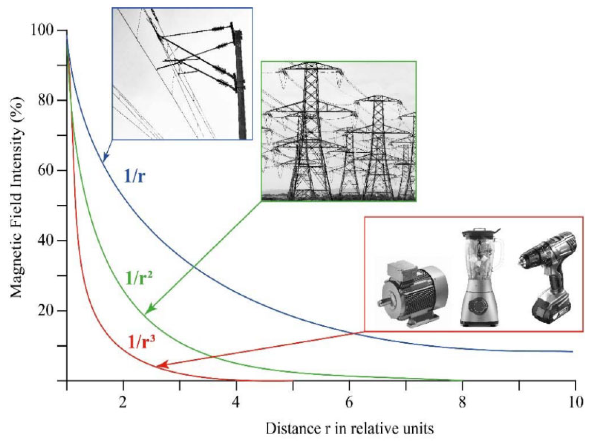
Depending on the exposure source and the distance from that source, magnetic field strengths might vary significantly. Depending on how well the opposing magnetic flux lines cancel each other out or how well the current-carrying lines are balanced, the rate at which the field intensity decreases with distance might differ from one source to another. At an increasing distance, fields from coils, magnets, or transformers degrade quickly by a factor of 1/r3. In power lines, partial field-cancelling causes the drop-off to be 1/r2 when currents flow in opposite directions. When there is an imbalanced current, the field intensity decreases more slowly than 1/r, as shown in Figure 1 [3].
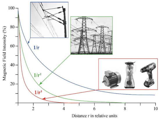
Figure 1.
The magnetic field intensity decreases with the growing distance from the field with fast (1/r3, 1/r2) or slow (1/r) drop-off [1].
The methodology of Extremely Low Frequency (ELF) measurements as defined by the International Telecommunication Union (ITU) is quite complex. Contrary to the measurement of high-frequency fields, extremely low-frequency fields present difficulties in their measurement, since at these frequencies the corresponding wavelengths exceed 100 m, thereby making it difficult to accurately measure in the near field [4]. It should be noted that the quantities of electric field strength, magnetic field strength, and equivalent power density are used to determine public exposure using suitable measuring devices. Regarding exposure to magnetic fields for public safety, the measured values should satisfy the mathematical Equation (1):
where Hi is the measurement of the magnetic field strength and HLi is the reference level for exposure at frequency i, as reported in Table 1, noting that the electromagnetic radiation limits according to Greek legislation correspond to 70% of the values that are described. The Weighted Peak Method (WPM) [5] was established by the ICNIRP 2010 guidelines for non-sinusoidal multiple-frequency fields. This method, incorporated into Directive 2013/35/EU [6], is required for the assessment of electrostimulation effects (non-thermal) at LF/ELF frequencies and is mandatory in all industrial applications for the safety of workers. The complex waveforms are weighted using a filter function that takes into account the waveforms’ phase, as described by the following equation [7]:
where t is the exposure time and Ai and ELi are the harmonic component amplitude and the exposure limit at ith harmonic frequency fi, respectively. The phase and filter angles of the field at the harmonic frequencies are also described by θi, φi. In addition, knowing that isotropic measurements should be along the X, Y, and Z axes, the total measured magnetic field Hi is described by Equation (3):

Table 1.
The Electric and Magnetic field reference levels in the European Union for general public exposure focused on Extreme Low Frequencies (ELF) [1,4].
Table 1.
The Electric and Magnetic field reference levels in the European Union for general public exposure focused on Extreme Low Frequencies (ELF) [1,4].
| Freq. Band | Electric Field Strength (V/m) | Magnetic Field Strength (A/m) | Magnetic Field Induction (μΤ) |
|---|---|---|---|
| 0–1 Hz | - | 3.2 104 | 4 104 |
| 1–8 Hz | 10,000 | 3.2 104/f2 | 4 104/f2 |
| 8–25 Hz | 10,000 | 4000/f | 5000/f |
| 0.025–0.8 kHz | 250/f | 4/f | 5/f |
| 0.8–3 kHz | 250/f | 5 | 6.25 |
| 3–150 kHz | 87 | 5 | 6.25 |
Where f, is the frequency in Hz or kHz, depending on how it is defined in the table cell that is in the same row and column of the frequency band. No E-field value is defined for frequencies less than 1 Hz, which are essentially static electric fields.
The continuing interest in making reliable measurements concerning public exposure to extremely low frequency (ELF) magnetic fields has led researchers to implement measurement devices for several years. Strong magnetic field sources can be detected using an ELF magnetic field meter by taking the necessary precautions [3,8]. The authors in [9] introduced a broadband magnetic field meter at the National Bureau of Standards (NBS), in 1985. The proposed meter has an isotropic probe unit consisting of three mutually orthogonal loops, each 10 cm in diameter, for magnetic field measurements up to 30 A/m. The novelty of this implementation was based on several improvements over available instruments for that time, such as the dynamic range of 44 dB, the flat frequency response (about ±1.0 dB), the isotropic response (about ±0.3 dB), and the overload capability, using only one probe head. The work in [10] introduced a sensor for isotropic magnetic and electric field measurements at frequencies less than 100 kHz, determining the electromagnetic interferences specialized in the audio frequency band. Three orthogonally oriented coils are used as an EMF sensor by the authors in [11], introducing a measurement method that enables a precise analysis of the field distribution. The study suggests a research technique that involves evaluating the strength of the electromagnetic field produced by the emitting coil in a Wireless Power Transfer (WPT) system in terms of both magnitude and direction.
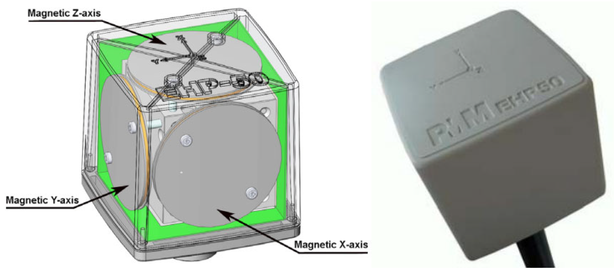
Nowadays, the technology of Electric and Magnetic Fields (EMF) meters has advanced considerably, offering engineers measurements with less uncertainty and the feature of remote equipment real-time monitoring. A professional solution for continuous monitoring of the electric and magnetic fields is provided by the Narda PMM EHP-50C probe analyzer [12,13] which can begin its acquisition by storing the data over 24 h in the operating frequency range of 5 Hz to 100 kHz. The analyzer features a variety of operating modes, including stand-alone mode without an external apparatus connection and cooperation with a Pocket-PC or Narda PMM 8053A portable display unit via fiber optic communication. In [14], another analyzer for measuring magnetic and electric fields in the workplace and public places is presented. The Narda EFA-300 provides field analysis using an FFT computation in combination with built-in, isotropic, magnetic field probes, as shown in Figure 2. The measurement process is intended to be substantially simplified by this new generation of equipment. The Narda EFA-300 incorporates the novel STD (Shaped Time Domain) mode in addition to detecting the RMS and peak values using the conventional filter technique, providing simple but reliable measurement even in complex environments. Regarding the magnetic field measurements, the Narda EFA-300 analyzer can detect fields from 1 nT to 31.6 mT over the operating frequency range of 5 Hz to 32 kHz.

Figure 2.
The internal structure of Narda PMM EHP-50C probe-analyzer for measurements of magnetic and electric fields over the frequency range 5 Hz to 100 kHz. The identical circular sensor probes are devoted to isotropic field measurements in the X, Y, and Z planes [13,14].
The authors in [15] introduced a broadband monitoring system for electromagnetic radiation exposure assessment, focused on RF frequencies (from radio and TV broadcastings, mobile telephony systems, Wi-Fi, and TETRA communications) in 2006. The proposed system called “SMS-K”, has been implemented for recording the E-field on a 24 h basis and sending the data to a central database via a GSM connection, as an early-stage EMF IoT platform. The real-time measurements are available via a web interface for citizens’ information within the framework of the “FASMA” project [16], supported by Wind Hellas Telecommunications SA. Thereinafter, other EMF monitoring projects called “HERMES” (2002) [17], “Pedion 24” (2006) [18], and “National Observatory of Electromagnetic Fields” (2015) [19] were developed for the continuous remote monitoring of electromagnetic radiation via a distributed network of fixed meters in Greece. In these projects, the Narda area monitors AMS-8061/G [20], AMB-8059 [21], and AMB-8057-03/G [22] were used only for E-field measurements at a wide operating frequency band (100 kHz–7 GHz). The measurement data from each stand-alone station are sent to the central database via the 3G/GPRS network for citizens’ information through the web portal of the project.
Undeniably, the existence of magnetic fields in urban and semi-urban environments could be used as another emergency energy source (under certain conditions) to power low-consumption devices, such as IoT sensors. Numerous locations could be beneficial for sensors where the magnetic flux density may be high enough to power a low-consumption WSN’s node, such as in high voltage substations, near railways, etc. Several published studies have covered the research on the magnetic flux density levels (B) under overhead power lines [23]. Researchers have verified that the flux density close to the ground is within legal limits. It stands to reason that different types of pylons will have varying overhead power line physical structures and typical line currents, leading to variable magnetic flux densities.
The authors in [24] propose a novel and efficient harvesting bow-tie coil to scavenge the magnetic field energy under overhead power lines, enabling the self-powering of a large number of sensors. In contrast to the typical way of placing the energy harvester on the power lines, the proposed coil does not need to be fastened to the line and may be put just above the ground, allowing for the powering of sensors with a larger volume.
The work in [25] presents a study of a generator that can continually charge batteries for pulsed communications, using the magnetic field created by high-voltage DC lines. In its implementation, no expensive magnetic material is required; however, several insulating issues, including the Corona phenomenon in transmission lines, should be taken into account for the proposed mounted harvester to be used in practice.
In [26], a free-standing inductive harvester for use in locations with ambient magnetic fields caused by far-off and/or difficult-to-reach conductors is presented. Researchers introduced a self-powered wireless sensor by utilizing ambient 50 Hz magnetic fields in High Voltage (HV) substations. The laboratory experimental results have shown that the proposed magnetic field harvester of the sensor can deliver a useful average power of 300 μW when placed in a magnetic flux density of 18 μT (RMS).
Based on numerous experiments using different inductors and combinations of current-carrying conductors, the authors in [27] offer a feasibility analysis of energy harvested from stray electromagnetic energy of household AC power lines. The results are encouraging since it is possible to harvest up to 2 mW of power using simple components for the harvester implementation.
The study in [28] presents two distinct configurations evaluated in situ along a Norwegian railway and in a controlled laboratory setting to support the viability of magnetic field energy harvesting (MF-EH) in electrical railways. The power output of the proposed system can reach up to 40.5 mW at 50 Hz when positioned near an emulated section of a railway carrying 200 A, based on the experimental measurements carried out at the laboratory. In a region with moderate traffic, the prototype system harvests 109 mJ from a single electric train, yielding an estimated daily energy output of 1.14 J.
Another magnetic field energy harvester (MF-EH) application for railways is presented in [29] to power wireless sensors for condition monitoring. In that study, an MFEH system was designed, enhanced, and tested for energy harvesting from the rail tracks’ traction return currents. The magnetic core was created using two flux collectors to partially enclose the rail track based on the dispersion of the magnetic field around the rail track. Measurements show that the MFEH’s power output was decreased by reducing eddy current loss by positioning it farther from the rail track. The experiment’s power output decreased from 5.05 to 1.6 W when the MFEH was relocated from a distance of 48 mm to 190 mm, where the eddy current loss was insignificant.
In this work, the implementation of an isotropic Extremely Low Frequency (ELF) IoT-based meter is presented. The proposed low-cost meter can measure the magnetic flux density from 100 nT with three identical sensor probes for isotropic field measurements in the X, Y, and Z planes, enhancing the work in [30]. The proposed device has an almost flat response across the frequency range from 40 to 10 kHz, detecting and measuring several magnetic field sources, including the public power supply network and its harmonic frequencies. In our approach, an Arduino UNO Wi-Fi Rev.2 board is used for data transferring from the sensor to the cloud as a complete IoT solution, supported by the Blynk application via Android and iOS operating systems or web interface. Furthermore, an ELF energy harvesting (EH) circuit was also proposed in our study for the utilization of the alternating magnetic fields (50 Hz) derived from the operation of several consumer devices such as transformers, power supplies, hair dryers, etc. using low-consumption applications.
The rest of this article is organized as follows: the proposed magnetic flux density meter operating principles are presented and analyzed in Section 2. Section 3 gives the full description of the electronic circuit (analogue section) of the proposed EMF meter. Section 4 is devoted to the description of the isotropic ELF sensor implementation. A demonstration of real-time ELF field monitoring as a proposed IoT solution via the Blynk application is presented in Section 5. Section 6 is devoted to the description of the magnetic field utilization derived from the operation of common-use electrical devices, such as a hair dryer at the laboratory using a proposed MFEH harvester, and finally, Section 7 includes the conclusions and a discussion on future work.
2. Magnetic Flux Density Meter Operating Principles
The induced electromotive force in any closed circuit is equal to the negative time rate of change in the magnetic flux contained in the circuit, according to Faraday’s Law of Electromagnetic Induction. Consequently, when magnetic flux flows through a coil, a voltage is generated across it, the magnitude of which is dependent on the field’s intensity rate and the enclosed surface area. In mathematical terms,
where Φ is the magnetic flux passing through the coil, A is the area enclosed by each turn of the coil, N is the total number of turns of the coil, B is the magnetic flux density of the field (magnetic field), and t is the time. Essentially, the time derivative of the magnetic flux density determines the rate of change in the magnetic flux density (a derivative of the magnetic flux concerning time).
It is considered that in space there is a harmonic (sinusoidal) magnetic field of the following form:
where B(t) is the instantaneous value of the magnetic flux density (function of time), Bo is the maximum value of the oscillating field, and f is the frequency of oscillation. From (4) and (5), we conclude that if a coil is placed into the harmonic field, a harmonic voltage E(t) will be induced at its terminals, which will be equal to the following:
We observe that the induced voltage is proportional to the geometric characteristics of the coil (A, N), the frequency f, and the field strength Bo. The harmonic term sin(2πft) indicates that voltage is a harmonic function of time and has a phase difference of 90° concerning the field. From (6), we observe that if the induced voltage E can be measured, the B field can be calculated, as long as the exact frequency f is known. In practice, when measuring the magnetic field of an arbitrary (unknown) source, its frequency is undetermined. The unknown frequency problem is resolved by multiplying both sides of Equation (7) by the absolute value of the G/G2πf term, where G is a constant for any specific frequency f, corresponding to amplifier voltage gain. Then, we will have:
By setting:
hence,
where V(t) is the instantaneous value of the harmonic voltage induced in the coil as a product by the absolute value of the G/2πf term. Referring to RMS terms (Root Mean Squared values) the RMS voltage (Vrms) is proportional to the RMS magnetic field density (Brms) and independent of the frequency [31,32]:
Therefore, it is easy to calculate the magnetic flux density (Brms) by measuring the voltage value (Vrms) with an analogue electronic device, i.e., a magnetic flux density meter. Figure 3 illustrates the block diagram of the proposed low-cost IoT magnetic flux density meter providing cloud-based services, as a comparative advantage among similar high-cost measurement equipment [13,14]. The proposed magnetic flux density meter’s electronic circuit is straightforward to implement, and the components have a low tolerance for measurement error minimization. A detector coil with well-defined geometric characteristics as a field sensor, an amplifier with voltage gain equal to G/2πf, an RMS detector, and a voltage display are required for a real circuit that makes use of Equation (9).
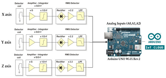
Figure 3.
The block diagram of the proposed isotropic IoT-based magnetic flux density meter. An Arduino UNO Wi-Fi Rev.2 board is used to provide 3 analog inputs for measurements in the X, Y, and Z axes and Wi-Fi connectivity, enhancing the previous version of the sensor [30].
In the proposed implementation, the Arduino UNO Wi-Fi Rev.2 board [33] is used instead of common voltmeters at analog outputs of the device, providing network connectivity for data transferring to the Blynk cloud [34], as a complete IoT EMF solution. The measured voltage values at three analogue inputs correspond to the magnetic field strength values in the X, Y, and Z axes, respectively, and can be displayed on any mobile device with Wi-Fi connectivity.
2.1. The Amplifier with G/2πf Gain
A circuit with a 1/f response is an integrator [35] (a low pass filter with a linear amplitude response and an ideal cut-off frequency of 0 Hz). An operational amplifier and several passive components can be used to create an almost ideal integrator. To achieve high gain value, one high-gain integrator or multiple amplifying stages in series with a reasonable-gain integrator are required. The second approach, in which the amplifier unit is employed before the integrator, is recommended for the proposed circuit. The detector requires high amplification to be sensitive without using any massive coil (since the output voltage for a reasonably sized coil is relatively small, in particular at low frequencies).
2.2. The RMS Detector
A section of the RMS detector is required for the implementation of a magnetic field meter that can measure RMS field values instead of average or peak values. A rectifier is used to extract the DC component and measure the RMS value of the integrators’ AC signal output.
The DC component of a rectified signal is shown to be directly proportional to the RMS value of the harmonic input signal. A half-wave rectified voltage Vs is considered during a full cycle (0–2π rad):
where Vm is the maximum value of the half-wave rectified voltage. The Fourier series of the previous function is as follows [36]:
and hence,
Moreover, we are aware that in half-wave rectified signal:
and,
The first term in (11) represents the DC component of the semi-rectified signal, the second term is the 1st harmonic (base frequency), and the remaining terms are higher-order harmonics, respectively. The following is assumed in a harmonic (sinusoidal) signal:
The RMS value of the input harmonic signal is equal to the π/ of the DC component of the semi-rectified signal. At the rectifier’s output (Vout), except the DC component, a large number of harmonics should be rejected. A low pass filter can be utilized to reject the harmonic frequencies. To achieve perfect harmonics rejection, the low pass filter’s cut-off frequency is required to be as low as possible. Consequently, the RMS detector can be realized consisting of a half-wave rectifier and a low-pass filter.
3. The Electronic Circuit of the Proposed EMF Magnetic Flux Density Meter (Analog Section)
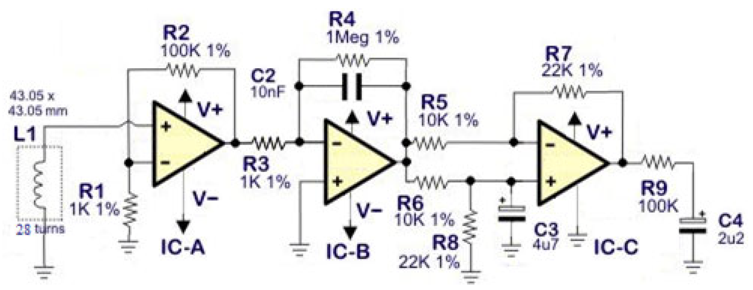
Figure 4 presents the proposed magnetic field meter’s basic electronic circuit (analog section).
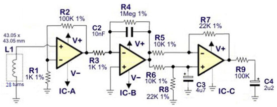
Figure 4.
The basic electronic circuit of the proposed magnetic flux density meter. For the implementation of an isotropic meter, 3 identical circuits are also needed for ELF measurements in the X, Y, and Z planes.
The Op-Amp A is used as a typical non-inverting amplifier with Ga gain:
The gain Ga is defined by R1 and R2 as described in Equation (16); it is equal to 101 and does not depend on frequency. Practically, the gain of the amplifier would be less than 101 for frequencies lower than 40 Hz. The design characteristics of the Op-Amp A limit the amplifier’s responsiveness at higher frequencies (the gain–bandwidth product). Nevertheless, from 40 Hz to 10 kHz, the amplifier response is almost flat, and the gain is approximately equal to the theoretical value with a potential error of less than 1 dB if 1% accuracy resistors are used for R1 and R2. The integrator follows the amplifier, implemented from Op-Amp B, R4, R3, and C2. The response of the integrator is inversely proportional to the frequency due to C2. If the integrator is analyzed as a typical inverse amplifier, it is observed that its gain Gb is equal to
The RF value is the impedance resulting from the parallel combination of resistor R4 and the Xc impedance (reactance) of C2. That is,
Knowing that Xc reactance is equal to:
By combining Equations (17)–(19), we find that:
It is noticed that the above equation is not exactly in the form of 1/f, mainly because our integrator is not ideal due to R4. Nevertheless, the product 2πfR4C2 is much larger than 1 for frequencies above 40 Hz and the “1” in the denominator can be omitted. Consequently, for frequencies above 40 Hz, the integrator’s gain becomes equal to:
The total gain of the amplifier and integrator chain would be the product of the Ga and Gb, namely:
From Equations (16), (21), and (22), we conclude that:
where:
Taking into consideration Equations (24) and (9), we observe that an AC voltage (Vrms) is produced at the output of the integrator, which is equal to
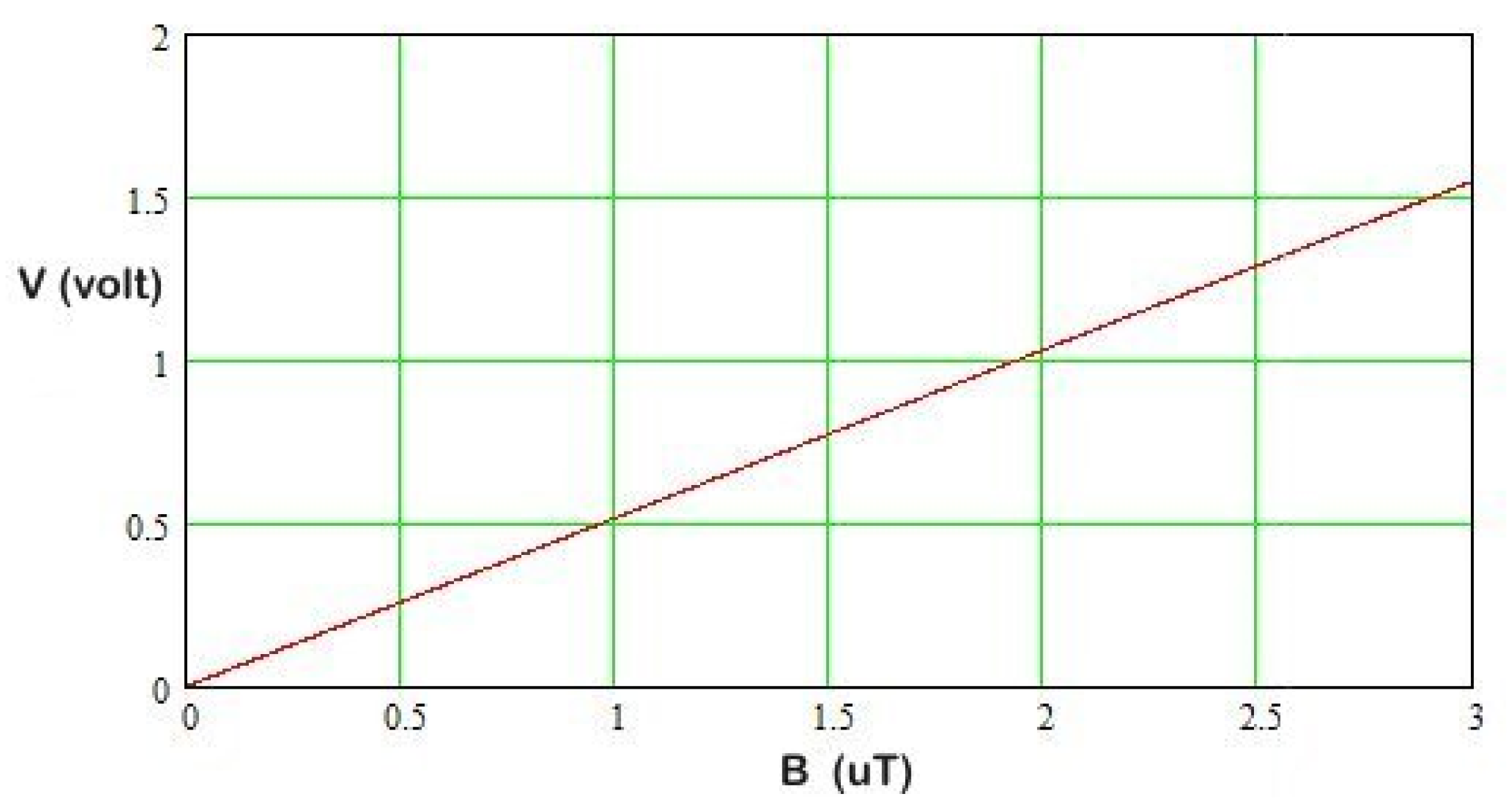
From Equation (25) we notice that the produced voltage is directly proportional to the field and independent of frequency, as shown in Figure 5. Based on the actual value calculation of the G constant, we observe that

Figure 5.
The output voltage of the proposed RMS detector is a function of the magnetic flux density.
The rectifier circuit is subsequent to the integrator, implemented from the Op-Amp C. Since there is no diode anywhere, the rectification circuit is uncommon. The rectification is carried out because the negative half-period of the signal is simply cut off. The Op-Amp C along with the resistors R5, R6, R7, and R8 is a typical differential amplifier circuit (subtraction). The voltage applied to the left end of R5 is subtracted from the voltage applied to the left end of R6. The output of the subtractor will always have a voltage equal to zero since the left edges of R5 and R6 are short-circuited, only in the case of DC. Contrariwise, for the AC signal, the capacitor C3 acts as a short circuit and grounds the non-inverting input of Op-Amp C. This method converts the subtractor into an inverting AC amplifier with an amplification of R7/R5 = 2.2.
The previous analysis demonstrates that Op-Amp C eliminates the DC component of the signal and amplifies the remaining AC signal by a factor of 2.2. Furthermore, Op-Amp C performs a half-rectification of the signal at 0 V reference level without negative supply voltage.
Consequently, it can only amplify the positive half-period of the signal, and during the negative half-period, its output is zero (i.e., half-phase rectification occurs). Op-Amp C output produces a semi-rectified signal containing a DC component and some harmonics (according to the Fourier series analysis mentioned above). The harmonics are filtered out from a simple low pass filter formed by R9 and C4. The cut-off frequency of this specific filter is equal to 1/2πR9C4 = 4.5 Hz, which is a very low one and the filter passes only the DC component. Normally, the DC component of a half-rectified signal is equal to /π of the RMS value of the input signal of the rectifier. The term /π is equal to about 1/2.2.
However, since we use amplification equal to 2.2 in the rectifier, we make the half-rectified signal have a DC component equal to the exact RMS value of the input signal (by cancelling out the 1/2.2 factor). The circuit has an analog output providing voltage equal to 0.1 mV/nT at the Analog to Digital (ADC) port of the Arduino WeMos D1 board. For instance, for a 2 μT field, there will be a voltage of 200 mV at the analogue output of the ELF meter. This output is provided on C4 terminals. C4, along with R9, forms a low-pass filter that extracts the DC component from the output of the rectifier as described above.
4. The Proposed ELF Isotropic Sensor Implementation
Winding a coil with a certain number of turns and specific dimensions may constitute the magnetic field probe of the ELF meter. Suppose that the Vrms voltage needs to be 1.2 V when the coil is placed inside a 2.3 μT (RMS) magnetic field. According to (25), the following equation should be satisfied:
In our initial prototype implementation [30], by choosing a coil with 100 turns, each turn should include an area of 516.6 × 10⁻⁶ m2. The desired area for a rectangular cross-section coil can be achieved if each turn is 43.05 mm × 12 mm. Thus, the meter coil in the initial design consisted of 100 turns of 43.05 mm × 12 mm rectangular cross-sections.
In this study, the sensor of the proposed meter consists of three identical square probes in vertical alignment, providing isotropic H-field measurements from the X, Y, and Z planes, respectively, as shown in Figure 6. Each probe should also satisfy Equations (25) and (27) considering that the initial dimensions should be appropriately changed to achieve the cubic structure of the proposed isotropic sensor. The coil of each axis probe consists of 28 turns of 43.05 mm × 43.05 mm square cross-sections to feed the identical electronic circuits of the meter (Figure 6b), to enhance the work in [30].
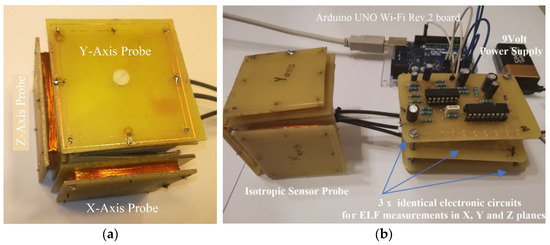
Figure 6.
(a) The sensor implementation of the proposed ELF meter consists of three identical square probes in vertical alignment, providing isotropic H-field measurements from the X, Y, and Z planes. (b) The main parts of the proposed magnetic field meter are the isotropic probes, the Arduino board, and the identical electronic circuits.
The measured incident magnetic field of the proposed sensor with three identical square coils is given by the following equation [14]:
where Vx, Vy, and Vz are the voltages at the outputs of the probe coils of the meter, and kx, ky, and kz are the respective coefficients that are derived from calibrating the device against other available laboratory-calibrated equipment, as the Narda PMM EHP-50C.
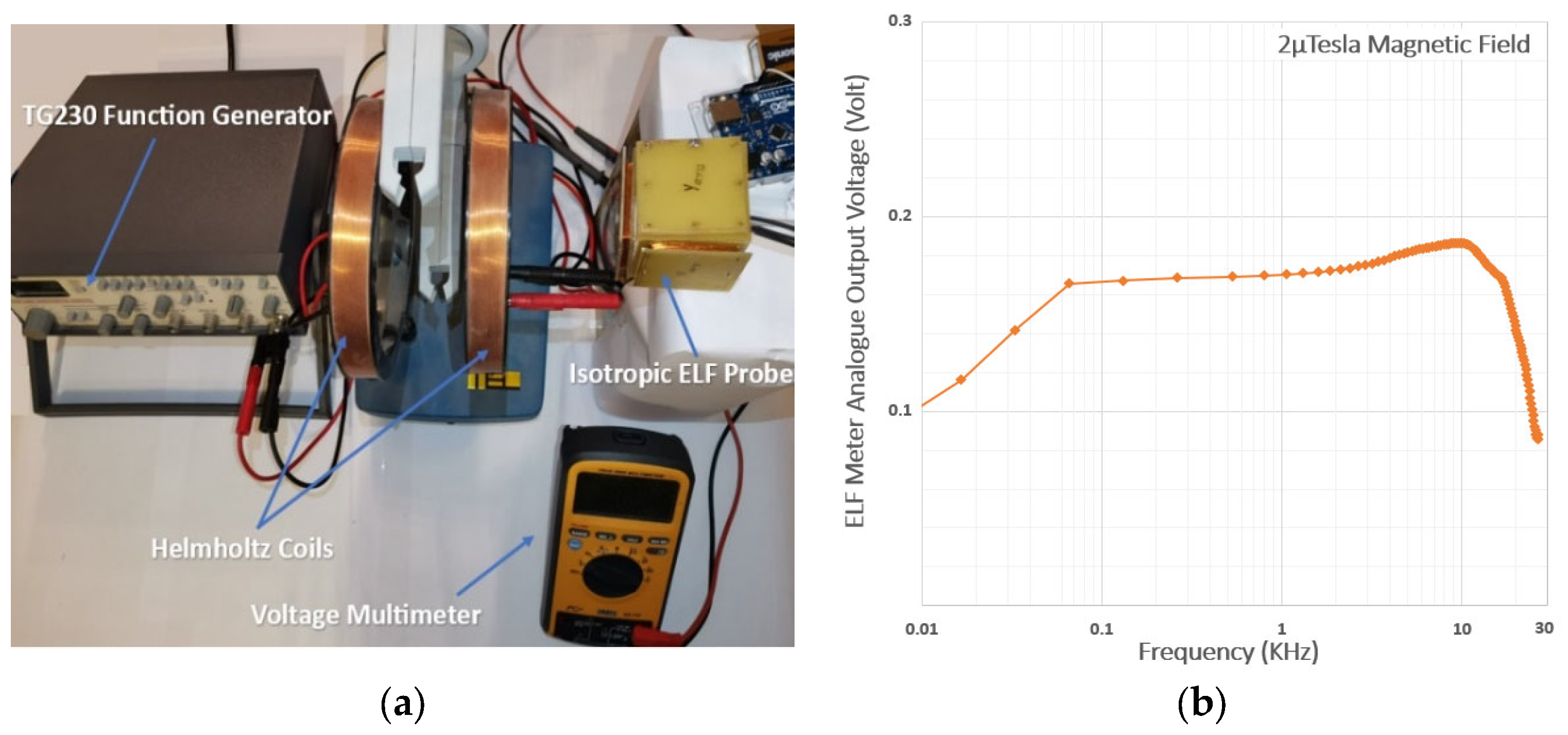
For the system’s frequency response validation, a TTi TG230 function generator was used to feed a pair of Helmholtz coils to provide a homogeneous magnetic field at the laboratory. Keeping constant the generator’s signal amplitude (and at the same time the intensity of the emitted magnetic field at about 2 μT), the operating frequency of the generator was changing in the ELF band (1 Hz–100 kHz) to achieve the frequency response curve of the proposed meter, as shown in Figure 7a. Experimental measurements show an almost flat response over the frequency range from 40 Hz to 10 kHz, as shown in Figure 7b, respectively. Table 2 shows the comparison of the proposed meter with similar high-precision and ultra-high-cost ELF measurement equipment solutions.
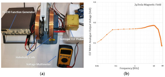
Figure 7.
(a) The frequency response validation via Helmholtz coils utilization feeding by a signal generator to provide a homogeneous magnetic field in the ELF band. (b) The frequency response curve of the meter.
5. IoT Application with Arduino UNO Wi-Fi Rev.2 board for Real-Time ELF Field Monitoring
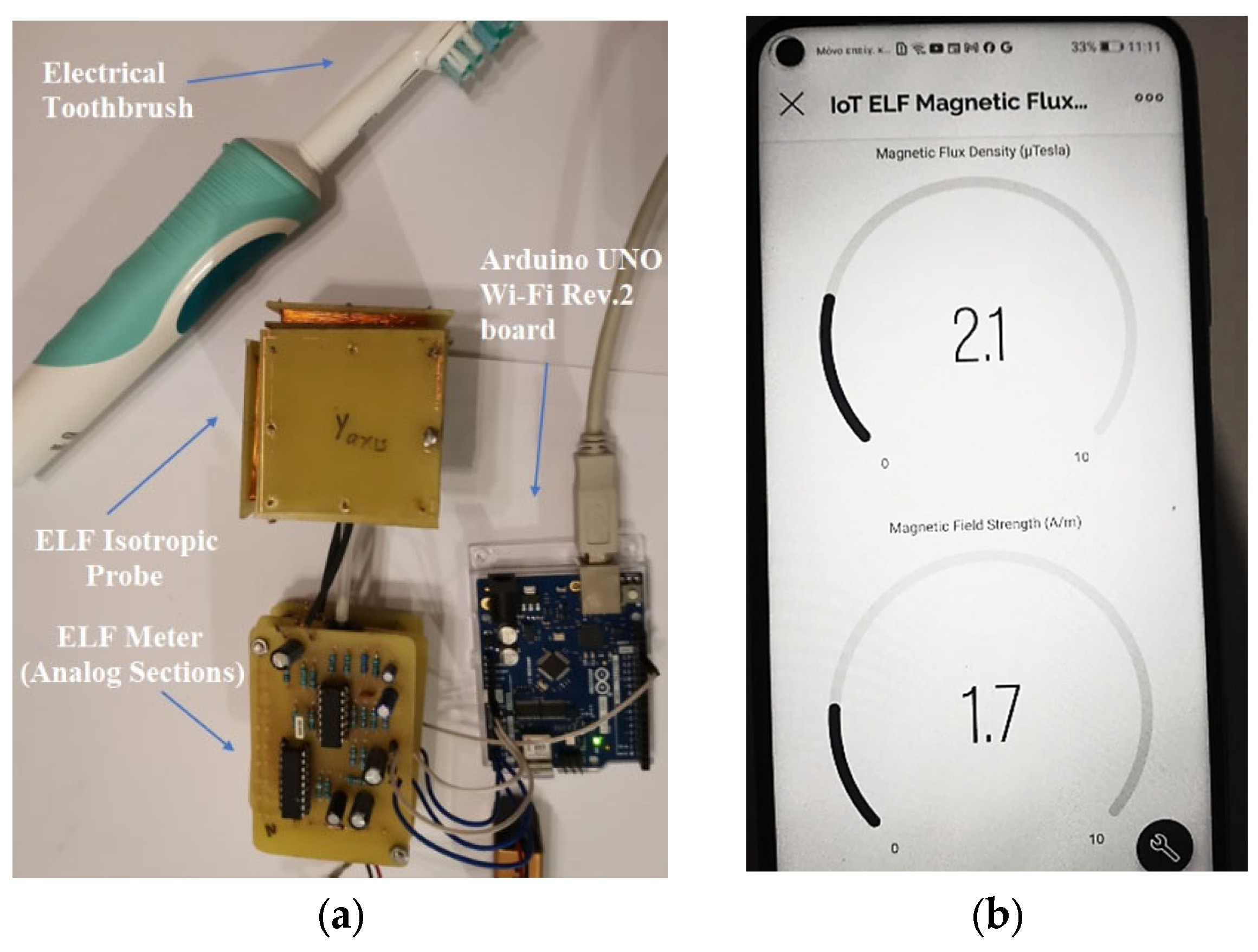
The value of the measured magnetic field can be displayed in real-time on any mobile device with Wi-Fi connectivity via the Blynk application [34] supported by Android and iOS platforms. An Arduino UNO Wi-Fi Rev.2 board with the embedded Wi-Fi Nina [33] module is used to provide three analogue inputs (ADC’s) for measurements in the X, Y, and Z axis, respectively to transfer data from the meter to the cloud as a complete EMF IoT solution [37], as shown in Figure 8. The Arduino Uno WiFi uses an 8-bit microprocessor and an onboard inertial measurement unit (IMU). Its Analog to Digital converter (ADC) has a 10-bit resolution, mapping input voltages between 0 and 5 V into integer values between 0 and 1023. This results in readings of 4.9 mV per unit (5 Volts/1024) on the Arduino UNO board.

Figure 8.
(a) Measuring the magnetic field exposure of an electrical toothbrush by the proposed IoT-based meter. (b) The isotropic ELF field strength values (in A/m and μTesla) are displayed on the Blynk application supported by the Android platform in a mobile phone with Wi-Fi connectivity, as a complete IoT solution.
The Blynk user interface can be displayed on the mobile terminal or the web portal and both the magnetic field strength H (A/m) and the corresponding flux density B (μTesla) values at the same time, using the following transformation formula:
where μr is the relative and μ0 is the free space magnetic permeability. Magnetic field levels up to 300 nT are considered within safe limits in most countries of the world. Several studies have shown that the field is regarded as potentially harmful from 400 nT to 1 μT, and dangerous from 1 μT and above [2,23]. Furthermore, the percentage magnetic field contribution (%) of each probe is available to the user to identify the plane direction (X, Y, or Z) of the incident magnetic field.
Table 2.
The comparison of the proposed meter with similar ELF measurement solutions.
Table 2.
The comparison of the proposed meter with similar ELF measurement solutions.
| Ref. | Freq. Response | Meas. Level | Connectivity | Type of Meas. |
|---|---|---|---|---|
| PMM EHP-50C [13] Narda EHP-50F [38] | 5 Hz–100 kHz 1 Hz–400 kHz | 1 nT–10 mT 0.3 nT–10 mT | Opt./USB Opt./USB | Magnetic/Electric Field Magnetic/Electric Field |
| Narda EFA-300 [14] | 5 Hz–32 kHz | 1 nT–31.6 mT | Opt./Serial | Magnetic/Electric Field |
| Study in [9] | 300 kHz–100 MHz | 125 nT–20 mT | Νot Μentioned | Magnetic Field |
| Study in [10] TM192D [39] | <100 kHz 30 Hz–20 kHz | Νot Μentioned up to 200 μΤ | Νot Μentioned USB | Magnetic/Electric Field Magnetic Field |
| This work | 40 Hz–10 kHz | 100 n–10 μT | WiFi, IoT (Blynk) | Magnetic Field |
6. Magnetic Field Energy Harvesting (MF-EH) from the Operation of Commercial-Use Electrical Devices
Several electric devices such as transformers, power supplies electric motors, hair dryers, etc., create powerful low-frequency magnetic fields capable of powering low-consumption applications (such as WSN sensors). In this section of our study, a Magnetic Field Energy Harvesting (MF-EH) circuit is also proposed for 50 Hz magnetic field utilization derived from these common-use electric devices in short distances. The proposed ELF energy harvester is based on an LC tuning circuit, with the same self-resonance frequency (fSRF) as the operation of the public electricity distribution network (50 Hz). The correlation between the resonance frequency (fSRF) of the circuit and the values of the tuning capacitor (Ctun) and the inductor coil (Ltun), respectively, is given by the Thomson Equations (30) and (31):
and therefore
The quality factor (Q) of the circuit is about 6.7, as calculated by Equation (32), as a series tuning circuit, where the resistance value of the coil (Rcoil) is about 160 Ohms. To achieve resonance at extremely low frequencies (ELF), a relatively high value of either the capacitance or the coil inductance is required. The higher value of the inductance makes the proposed circuit more sensitive for energy harvesting from alternating magnetic fields of 50 Hz.
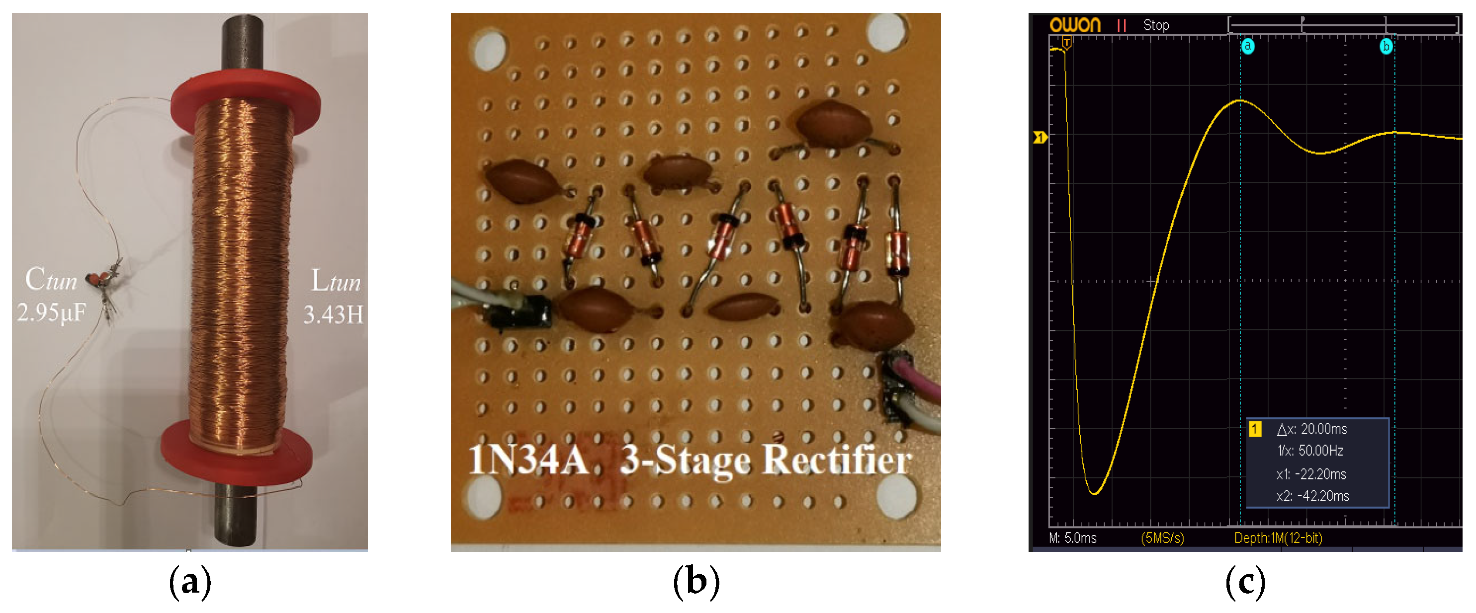
For our implementation, a value of 3.4H has been chosen for the inductance achieved by hundreds of turns of 0.3 mm insulated copper wire, combined with the addition of an iron core in the resonant coil, as shown in Figure 9a. Thus, the capacitor value (Ctun) of the tuning circuit is required to be about 2.9 μF to achieve oscillation at the resonance frequency of 50 Hz. The parametric study of the components was carried out at the laboratory, recording the genesis of the descending oscillation using a digital oscilloscope until the desired resonance frequency of 50 Hz (fSFR) was reached, as shown in Figure 9c.

Figure 9.
(a) The coil of the LC tuning circuit of the proposed ELF harvester is made by hundreds of turns of 0.3 mm insulated copper wire to achieve 50 Hz resonance frequency. (b) 3-Stage Cockcroft-Walton rectifier. (c) The genesis of the descending oscillation using a digital oscilloscope at the laboratory for the resonance frequency fine-tuning at 50 Hz.
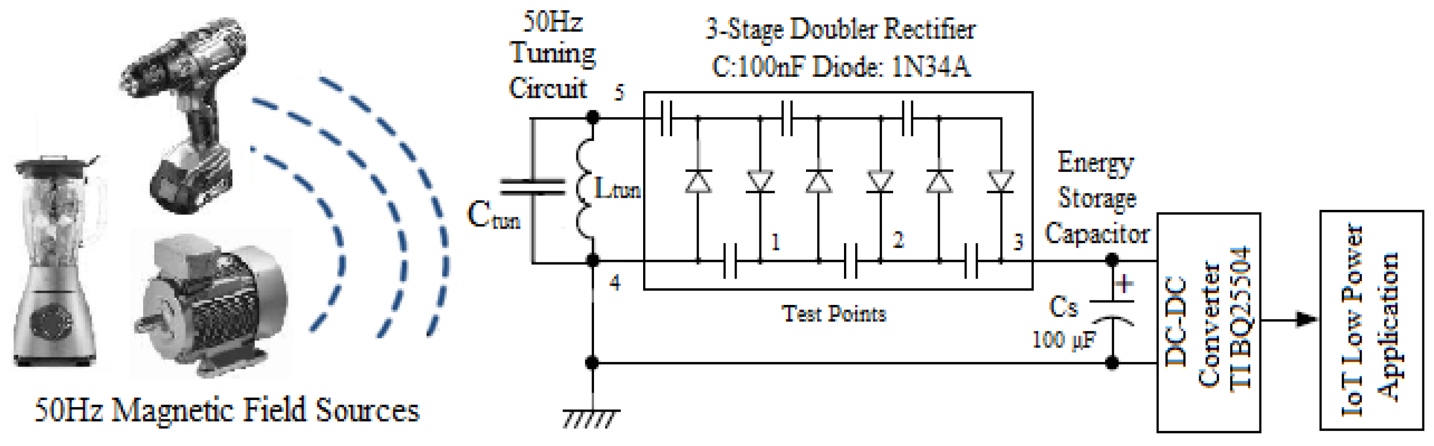
The proposed circuit was tested for alternating magnetic field energy harvesting from electric devices such as transformers, power supplies, etc. in the laboratory. The output of the tuned LC circuit indicates the rectifier of the proposed system. A 3-stage germanium diode-based (1N34A) Cockcroft-Walton rectifier [40] with 100 nF blocking capacitors was used for DC conversion, as shown in Figure 9b. In the prototype, the ability to monitor the output voltage of each rectifier stage is also provided to obtain additional experimental measurements and select the most efficient number of stages at test points 1 to 3, respectively. As already mentioned, the magnetic field intensity decreases with the growing distance from the fields caused by coils, magnets, or transformers by a factor of 1/r3, resulting in harvesting voltage drop, respectively. For this limitation compensation, the Texas Instruments BQ22504 DC-DC boost converter [41] could be used as an optional stage of the system for the necessary voltage raising providing power to low-consumption devices, as shown in the block diagram in Figure 10. The BQ25504 is a high-efficiency ultra-low-power boost converter, designed for energy harvesting applications. This device was created with efficiency in acquiring and managing microwatts (µW) to milliwatts (mW) of power, produced by several DC harvesting sources. It is feasible to start with a VIN as low as 600 mV and continue energy harvesting until the VIN is higher or equal to 130 mV. A storage capacitor (Cs) of 100 μF is placed to store the harvested energy from magnetic field sources as a capacitor-based EH system [42,43], feeding the BQ22504 boost converter for powering low-consumption applications.
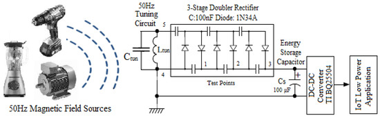
Figure 10.
The electronic diagram of the proposed ELF energy harvesting system and some of the magnetic field sources. The test points 1, 2 and 3 corresponds to the individual stages of the rectifier.
7. MF-EH Experimental Results
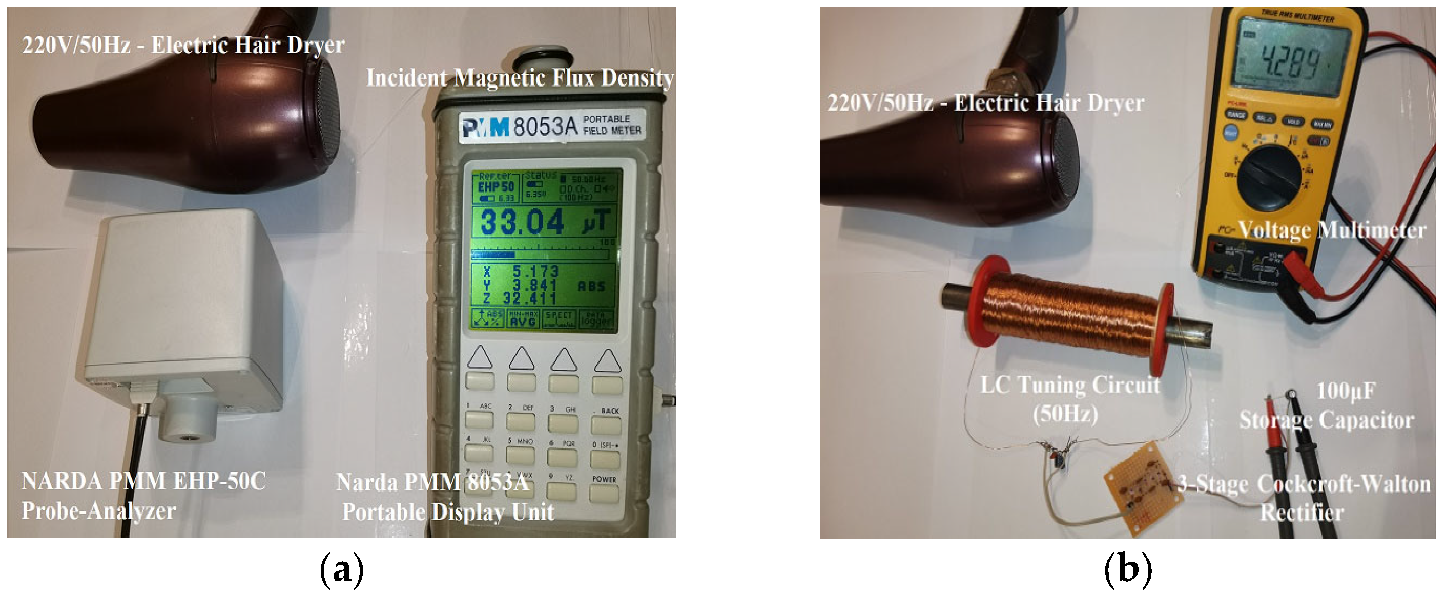
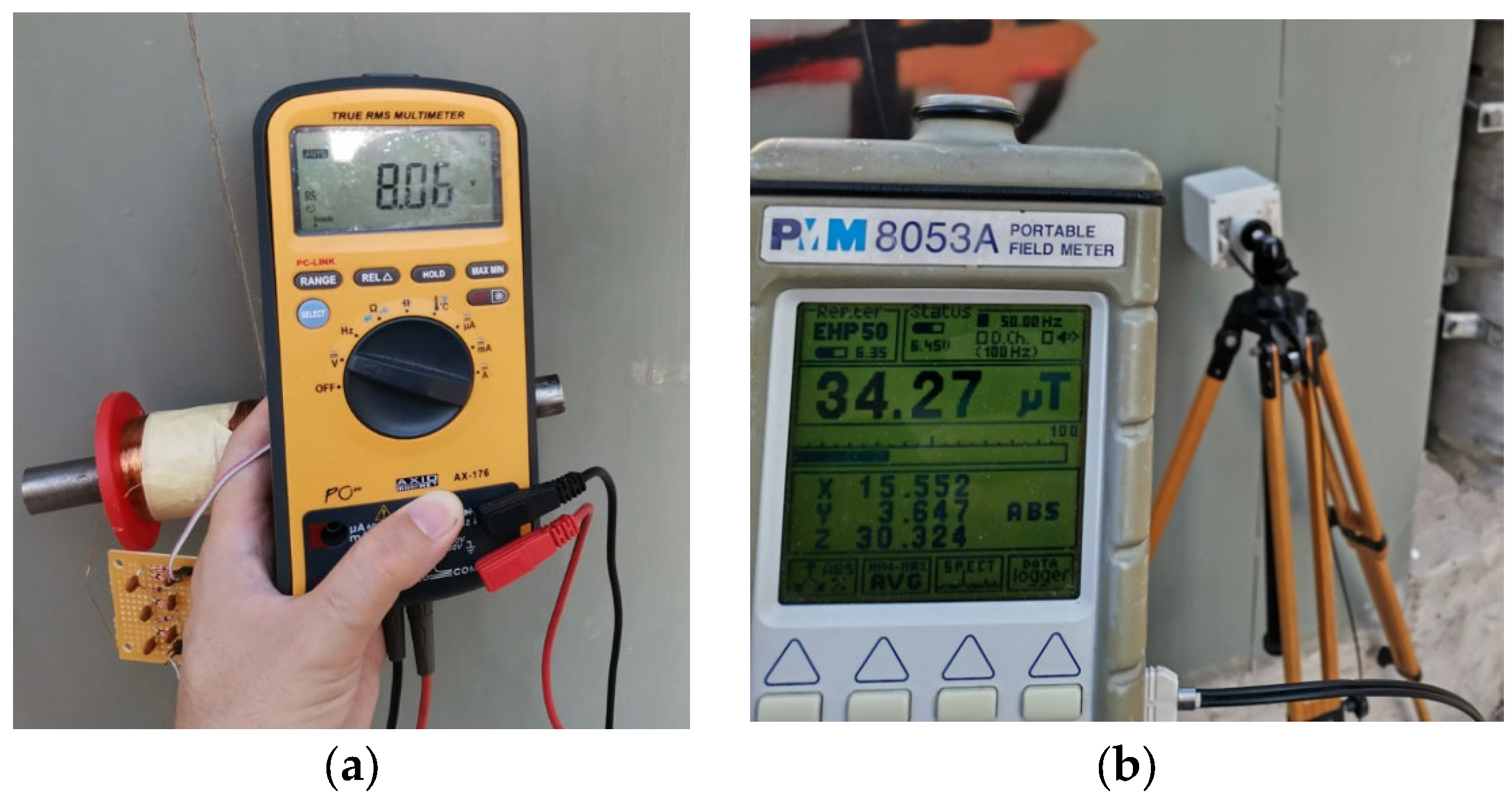
The experimental measurements showed that at a relatively close distance from the tested magnetic source (hair dryer), the (DC) harvesting voltage can reach up to 4.2 volts, as shown in Figure 11b. The storage capacitor (Cs) of the system can be fully charged in 3 min with a 33 μΤ magnetic field caused by the operation of an electric hair dryer, as depicted in Figure 12 and Figure 11a, respectively. The storage capacitor’s (Cs) charging curves demonstrate that the maximum charging voltage (Vmax) is proportional to the ambient magnetic field strength, as shown in Figure 12. The dynamic behaviour of the rectifier diodes depends to a large extent on the levels of the received signal, consequently affecting the equivalent resistance of the rectifier circuit (Rthevenin), with the change in the time constant charging (tcharge) as a final result. The experimental measurements were also extended to the utilization of the alternating magnetic field near medium voltage substations of the electrical public distribution network. Firstly, magnetic field strength measurements were performed around the perimeter of the metal cabin where the transmission lines of the distribution network are driven, with the Narda EHP-50C PMM field meter, detecting magnetic field values of up to 60 μT (at peak time within an urban environment). The experimental setup developed an (open circuit) voltage that reached 8 Volts at points where the magnetic field density was maximum, as shown in Figure 13a,b, respectively. It should be noted that the harvesting voltage is a function of the spatial placement of the tuning circuit of the device, as it is not possible to harvest energy isotopically using the original design of the prototype (axes X, Y, Z).
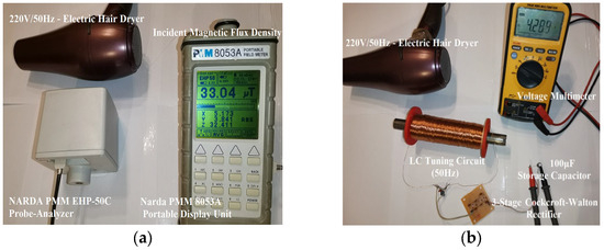
Figure 11.
(a) The irradiated magnetic flux density value can reach up to 33 μT, near a common-use hair dryer, as shown by the Narda PMM EHP-50C analyzer. (b) Experimental measurements showed that the (DC) harvesting voltage can reach up to 4.2 volts from this magnetic field value using the proposed MFEH system.
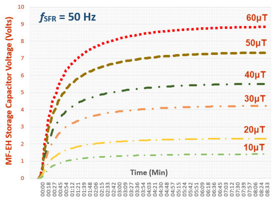
Figure 12.
Charging curves of the storage capacitor (100 μF) as a function of the intensity of the changing magnetic field (50 Hz) environment. The maximum voltage (Vmax) of the storage capacitor depends on the intensity of the magnetic field, having also an effect on the charging time constant.
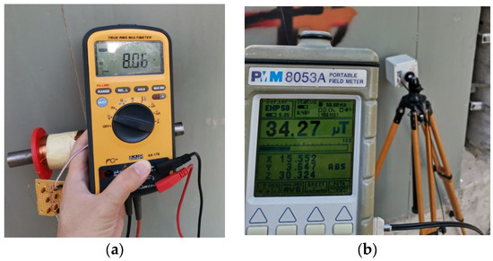
Figure 13.
(a) The harvesting voltage is up to 8 Volt near the metal cabin in a medium voltage substation of the public electricity distribution network using the proposed MF-EH. (b) Τhe average value of the magnetic flux density is about 34 μT, as shown from experimental measurements in a metal cabin of a medium voltage substation within an urban fabric during peak hours.
8. Conclusions and Future Aspects
This study presents the implementation of an isotropic Extremely Low Frequency (ELF) IoT-based meter, as enhanced in our previous work [30]. The prototype circuit can measure the magnetic flux density from 100 nT up to 10 μT with 3 square identical sensor probes in vertical alignment, providing isotropic field measurements in the X, Y, and Z planes. The meter has a flat response across the operating frequency range from 40 Hz to 10 kHz. The proposed low-cost device can measure all magnetic fields from sources such as transformers, electric motors, heaters, hair dryers, and power supply network and their harmonic frequencies. An Arduino UNO Wi-Fi Rev.2 board with the integrated WiFiNINA module is responsible for data transferring from the sensor to the cloud, as a complete IoT solution. The measured field can be displayed on any mobile device with Wi-Fi connectivity, supported by the Blynk application via Android and iOS operating systems or web interface. As a future aspect, an improved version of the proposed isotropic meter could be used to implement a distributed EMF IoT sensors network to remotely monitor ELF magnetic field exposure in an interestingly high-risk area. Furthermore, the Arduino FFT feature could also depict the measured magnetic field strength within its harmonic frequencies in future improved implementation. The presence of magnetic fields in urban and semi-urban areas may be exploited as an emergency backup energy source to power low-consumption electronic devices, like Internet of Things (IoT) sensors. In our study, an ELF energy harvesting (EH) circuit implementation was also presented for the utilization of the alternating magnetic field (50 Hz) derived from the operation of transformers, power supplies, and other consumer devices both at the laboratory and at near-distance of medium voltage substations of the electrical public distribution network. Experimental measurements showed that the (DC) harvesting voltage can reach up to 4.2 volts with a magnetic field of 33 μΤ, which is caused by the operation of an electric hair dryer, and can fully charge the 100 μF storage capacitor (Cs) of the proposed EH system in about 3 min. The usage of a higher value of coil inductance (with a simultaneous change in the capacitance of the capacitor) causes a more sensitive circuit for efficient energy harvested from the magnetic fields of the devices, operating in power frequency (50 Hz).
Author Contributions
Conceptualization, M.G.T.; methodology, M.G.T. and G.A.A.; software M.G.T.; validation, M.G.T.; formal analysis, M.G.T., G.A.A., D.V., T.Y. and D.S.; investigation, M.G.T., G.A.A., D.V., T.Y. and D.S.; resources, M.G.T., G.A.A., D.V., T.Y. and D.S.; data curation, M.G.T.; writing—original draft preparation, M.G.T.; writing—review and editing, M.G.T., D.V., T.Y. and D.S.; visualization, M.G.T.; supervision, D.V., T.Y. and D.S.; project administration, D.V.; funding acquisition, D.V. All authors have read and agreed to the published version of the manuscript.
Funding
The present article is part of the PhD thesis of M.G.T. The implementation of the doctoral thesis was co-financed by Greece and the European Union (European Social Fund-ESF) through the Operational Programme “Human Resources Development, Education and Lifelong Learning” in the context of the Act “Enhancing Human Resources Research Potential by undertaking a Doctoral Research” Sub-action 2: IKY Scholarship Programme for PhD candidates in the Greek Universities (MIS-5113934).

Institutional Review Board Statement
Not applicable.
Informed Consent Statement
Not applicable.
Data Availability Statement
The data used in this study are available upon request from the corresponding author. The data will be publicly available after the completion of the PhD thesis.
Conflicts of Interest
The authors declare that there is no conflict of interest.
References
- Maffei, M.E. Magnetic Fields and Cancer: Epidemiology, Cellular Biology, and Theranostics. Int. J. Mol. Sci. 2022, 23, 1339. [Google Scholar] [CrossRef] [PubMed]
- Park, J.K.; Jeong, E.H.; Seomun, G.A. Extremely Low-Frequency Magnetic Fields Exposure Measurement during Lessons in Elementary Schools. Int. J. Environ. Res. Public Health 2020, 17, 5284. [Google Scholar] [CrossRef] [PubMed]
- Metz, R. Build this Magnetic Field Meter. In Radio Electronics-Electronic Experimenter’s Handbook; 1993; Available online: https://www.industrial-electronics.com/re_elec-exp-hndbk_magnetic.html (accessed on 9 November 2023).
- Stratakis, D.; Miaoudakis, A.; Katsidis, C.; Zacharopoulos, V.; Xenos, T. On the uncertainty estimation of electromagnetic field measurements using field sensors: A general approach. Radiat. Prot. Dosim. 2009, 133, 240–247. [Google Scholar] [CrossRef] [PubMed]
- ICNIRP. Guidelines for limiting exposure to time-varying electric and magnetic fields (1 Hz to 100 kHz). Health Phys. 2010, 99, 818–836. [Google Scholar] [CrossRef]
- EU. Directive 2013/35/EU of the European Parliament and of the Council of 26 June 2013 on the minimum health and safety requirements regarding the exposure of workers to the risks arising from physical agents (electromagnetic fields). Off. J. Eur. Union 2013, 2013, 1–21. [Google Scholar]
- Trentadue, G.; Zanni, M.; Martini, G. Assessment of low-frequency magnetic fields in electrified vehicles. In EUR 30198 EN; Publications Office of the European Union: Luxembourg, 2020. [Google Scholar]
- Bonekamp, H. Magnetic—Field Meter. In Elektor Magazine; 1997; p. 26. Available online: https://www.elektormagazine.com/magazine/elektor-199701/33758 (accessed on 9 November 2023).
- Cruz, J.; Driver, L.; Kanda, M. Design of the National Bureau of Standards Isotropic MagneticField Meter (MFM-10) 300 kHz to 100 MHz. In Technical Note (NIST TN); National Institute of Standards and Technology: Gaithersburg, MD, USA, 1985. [Google Scholar]
- David, V.; Antoniou, M.; Cretu, M.; Salceanu, A. An isotropic sensor for the measurement of low frequency electric and magnetic fields. In Proceedings of the Conference Digest Conference on Precision Electromagnetic Measurements, Ottawa, ON, Canada, 16–21 June 2002; pp. 20–21. [Google Scholar]
- Petrascu, C.; Tulbure, A.; Topa, V. Implementation of an Accurate Measurement Method for the Spatial Distribution of the Electromagnetic Field in a WPT System. Appl. Sci. 2023, 13, 5773. [Google Scholar] [CrossRef]
- Narda PMM 8053A; The Solutions for Every Electrosmog Problem from 5 Hz up to 40 GHz, User Manual. 2004. Available online: http://www.gruppompb.uk.com/public/upload/8053BEN-40918-3.16.pdf (accessed on 9 November 2023).
- Narda EHP-50C; Electric and Magnetic Field Probe-Analyzer from 5 Hz up to 100 kHz, User Manual. 2009. Available online: https://www.gruppompb.com/public/upload/manuale-v-1_32-ehp-50-c.pdf (accessed on 9 November 2023).
- Narda EFA-300; For Isotropic Measurement of Magnetic and Electric Fields, User Manual. 2013. Available online: https://www.narda-sts.com/cn/%E6%9C%8D%E5%8A%A1%E4%B8%8E%E6%94%AF%E6%8C%81/%E4%BA%A7%E5%93%81%E8%B5%84%E6%96%99/efa-cn/pd/pdfs/24104/eID/ (accessed on 9 November 2023).
- Mavromatis, F.; Boursianis, A.; Samaras, T.; Koukourlis, C.; Sahalos, J.N. A Broadband Monitoring System for Electromagnetic-Radiation Assessment. IEEE Antennas Propag. Mag. 2009, 51, 71–79. [Google Scholar] [CrossRef]
- “FASMA” EMF Project—Wind Telecommunications SA. Available online: https://www.wind.gr/ (accessed on 25 September 2023).
- “HERMES” EMF Project—Vodafone Telecommunications. Available online: http://www.hermes.ntua.gr/ (accessed on 25 September 2023).
- “Pedion 24” EMF Project—Cosmote Telecommunications. Available online: http://www.pedion24.gr/ (accessed on 25 September 2023).
- “National Observatory of Electromagnetic Fields-NOEF” EMF Project-Greek Atomic Energy Commission. Available online: https://paratiritirioemf.eeae.gr (accessed on 25 September 2023).
- Narda AMS-8061; Selective Area Monitor—User Manual. Available online: https://www.narda-sts.com/en/selective-emf/ams-8061/pd/pdfs/23219/eID/ (accessed on 25 September 2023).
- Narda AMB-8059; Multi-Band Area Monitor—User Manual. Available online: https://www.narda-sts.com/ (accessed on 25 September 2023).
- Narda AMB 8057-03/G; Broadband Area Monitor—User Manual. Available online: https://www.narda-sts.com/en/selective-emf/ (accessed on 25 September 2023).
- Miroslav, Š.; Lipovský, P.; Draganová, K.; Ňák, J.; Milan, O.; Marek, Š.; Rudolf, A.; Rozenberg, R. Low Frequency Magnetic Fields and Safety. In Proceedings of the 17th Czech and Slovak Conference on Magnetism, Košice, Slovakia, 3–7 June 2019; Acta Physica Polonica Proceedings, A. Volume 137, pp. 693–696. [Google Scholar]
- Yuan, S.; Huang, Y.; Zhou, J.; Xu, Q.; Song, C.; Thompson, P. Magnetic Field Energy Harvesting Under Overhead Power Lines. IEEE Trans. Power Electron. 2015, 30, 6191–6202. [Google Scholar] [CrossRef]
- Guo, F.; Hayat, H.; Wang, J. Energy harvesting devices for high voltage transmission line monitoring. In Proceedings of the 2011 IEEE Power and Energy Society General Meeting, Detroit, MI, USA, 24–29 July 2011; pp. 1–8. [Google Scholar]
- Roscoe, N.M.; Judd, M.D. Harvesting Energy from Magnetic Fields to Power Condition Monitoring Sensors. IEEE Sens. J. 2013, 13, 2263–2270. [Google Scholar] [CrossRef]
- Gupta, V.; Kandhalu, A.; Ragunathan (Raj), R. Energy harvesting from electromagnetic energy radiating from AC power lines. In Proceedings of the 6th Workshop on Hot Topics in Embedded Networked Sensors (HotEmNets ‘10), Killarney, Ireland, 28–29 June 2010; pp. 1–6. [Google Scholar]
- Espe, A.E.; Haugan, T.S.; Mathisen, G. Magnetic Field Energy Harvesting in Railway. IEEE Trans. Power Electron. 2022, 37, 8659–8668. [Google Scholar] [CrossRef]
- Yang, K.; Zheng, C.; Tingwen, R.; Tim, L.; Ben, A.; Bimal, N.; Meiling, Z. Magnetic field energy harvesting from the traction return current in rail tracks. Elsevier J. Appl. Energy 2021, 292, 116911. [Google Scholar]
- Tampouratzis, M.G.; Adamidis, G.; Vouyioukas, D.; Yioultsis, T.; Stratakis, D. IoT-based ELF Magnetic Flux Density Meter. In Proceedings of the 3rd International Conference on Control, Artificial Intelligence, Robotics and Optimization (ICCAIRO), Ierapetra, Greece, 11–13 April 2023. [Google Scholar]
- Gordon, D.; Brown, R.; Haben, J. Methods for measuring the magnetic field. IEEE Trans. Magn. 1972, 8, 48–51. [Google Scholar] [CrossRef]
- Sebo, S.A.; Caldecott, R.; Kasten, D.G.; Wang, S.; Leach, J.A.; Vinh, T. Magnetic flux density measurement techniques to analyze 345 kV circuit breaker maintenance operations. In Proceedings of the IEEE Porto Power Tech Conference, Porto, Portugal, 10–13 September 2001; Volume 4, p. 5. [Google Scholar]
- WiFiNINA Arduino Module. Available online: https://docs.arduino.cc/ (accessed on 25 September 2023).
- Blynk IoT Platform: For Businesses and Developers. Available online: https://blynk.io/ (accessed on 25 September 2023).
- Chaniotakis, M.; Cory, D. 6.071 Introduction to Electronics, Signals and Measurement; Massachusetts Institute of Technology: Cambridge, MA, USA, 2006. [Google Scholar]
- Sethuraman, J. A Note on Fourier Series of Half Wave Rectifier, Full Wave Rectifier, and Unrectified Sine Wave; Vinayaka Mission’s Kirupananda Variyar Engineering College: Salem Tamil Nadu, India. Available online: https://www.academia.edu/7007379/A_NOTE_ON_FOURIER_SERIES_OF_HALF_WAVE_RECTIFIER_FULL_WAVE_RECTIFIER_AND_UNRECTIFIED_SINE_WAVE (accessed on 9 November 2023).
- Getting Started with the Arduino IoT Cloud. Available online: https://docs.arduino.cc/arduino-cloud/guides/overview/ (accessed on 25 September 2023).
- Narda EHP-50F; Electric and Magnetic Field Probe-Analyzer from 1 Hz Up to 400 kHz—User Manual. 2021. Available online: https://www.narda-sts.com/fileadmin/Produktliteratur_BAs_Software/EHP-50F/Bedienungsanleitung_Commands/Manual_EHP50F_EN.pdf (accessed on 9 November 2023).
- LF Tenmars TM-192/TM-192D, 3-Axis EMF Magnetic Field Meter—User Manual. 2020. Available online: https://www.radonshop.com/mediafiles/Anleitungen/Elektrosmog/Tenmars_TM-192/Tenmars_TM-192_ManualEN.pdf (accessed on 9 November 2023).
- Jaiwanglok, A.; Eguchi, K.; Julsereewong, A.; Pannil, P. Alternative of high voltage multipliers utilizing Cockcroft–Walton multiplier blocks for 220 V and 50 Hz input. J. Energy Rep. 2020, 6, 909–913. [Google Scholar] [CrossRef]
- Texas Instruments BQ25504 “Ultra-Low-Power Boost Converter with Battery Management for Energy Harvester Applications” —User Manual. 2023. Available online: https://www.ti.com/lit/ds/symlink/bq25504.pdf (accessed on 9 November 2023).
- Tampouratzis, M.G.; Vouyioukas, D.; Stratakis, D. Discone Rectenna Implementation for Broadband RF Energy Harvesting. In Proceedings of the 8th International Conference on Modern Circuits and Systems Technologies (MOCAST), Thessaloniki, Greece, 13–15 May 2019. [Google Scholar]
- Tampouratzis, M.G.; Vouyioukas, D.; Stratakis, D.; Yioultsis, T. Use Ultra-Wideband Discone Rectenna for Broadband RF Energy Harvesting Applications. Int. J. Technol. 2020, 8, 21. [Google Scholar] [CrossRef]


Disclaimer/Publisher’s Note: The statements, opinions and data contained in all publications are solely those of the individual author(s) and contributor(s) and not of MDPI and/or the editor(s). MDPI and/or the editor(s) disclaim responsibility for any injury to people or property resulting from any ideas, methods, instructions or products referred to in the content. |
© 2023 by the authors. Licensee MDPI, Basel, Switzerland. This article is an open access article distributed under the terms and conditions of the Creative Commons Attribution (CC BY) license (https://creativecommons.org/licenses/by/4.0/).