Nonlinear Dynamics and Energy Harvesting of a Two-Degrees-of-Freedom Electromagnetic Energy Harvester near the Primary and Secondary Resonances

Abstract

Energy harvesting is a useful technique for various kinds of self-powered electronic devices and systems as well as Internet of Things technology. This study presents a two-degrees-of-freedom (2DOF) electromagnetic energy harvester that can use environment vibration and provide energy for small electronic devices. The proposed harvester consists of a cylindrical tube with two moving magnets suspended by a magnetic spring mechanism and a stationary coil. In order to verify the theoretical model, a prototype electromagnetic harvester was constructed and tested. The influence of key parameters, including excitation acceleration, response to a harmonic frequency sweep, and electromechanical coupling on the generated characteristics of the harvester, was investigated. The experimental and theoretical results showed that the proposed electromagnetic energy harvester was able to increase the resonance bandwidth (60–1200 rad/s) and output power (0.2 W). However, due to strong nonlinearity, an unstable region occurred near the main first resonance, which resulted from the Neimark–Sacker bifurcation.

1. Introduction

One of the main challenges of Internet of Things (IoT) technology is to find adequate power supply [1]. The current trend is integrating the IoT system with sensors and wireless communication components. Consequently, there are higher requirements for wireless communication, sensor miniaturization, and reduced power consumption of electronic devices. Energy harvesting is a promising technique that converts unused abundant environmental energy into electrical energy. Therefore, kinetic (or vibration) energy harvesting systems are considered potential candidates to supplement electrical energy sources for self-powered sensors, IoT technology, and wearable microdevices (MEMS). All harvesters use transducer mechanisms to convert mechanical energy into electricity. The most popular ones are electromagnetic, piezoelectric, and electrostatic.

Electromagnetic harvesters (EHs) appear to be extremely promising in practice. One possible explanation for this is the high mechanical robustness of these mass-spring-damper constructions, which means that they can be installed with coils and magnets rather than with fragile piezoelectric crystals [2] and that they can be applied at low frequencies. Most EHs rely on magnets oscillating in a coil suspended by a spring or magnetic levitation. In the paper [3], various technologies were used for the fabrication of the harvester, and insights into the circuits used in real applications were given. That study primarily focused on design configurations, construction parameters, modeling, and experimental validation of transduction mechanisms and energy outcomes. Spreemann et al. [4] demonstrated that an appropriate electromagnetic harvester architecture could improve efficiency by about 10%.

Magnetic levitation energy harvesters are interesting due to their capacity for operation in a low-frequency bandwidth. Therefore, they can be effectively applied in pendulum vibration harvester/absorber systems [5,6]. These harvesters have a simple and easy-to-maintain design, which eliminates the need for mechanical components such as springs. These systems have a non-linear stiffness profile due to magnetic forces producing a nonlinear frequency response, allowing more power to be collected over a larger frequency range. A comprehensive and systematic analysis of 21 design configurations of electromagnetic energy harvesters with magnetic levitation architectures is given in [7]. These are classified into four types based on the number of coils and permanent magnets: single coil and single levitating magnet [8,9], single coil and multiple levitating magnets [10,11], multiple coils and single levitating magnet [12,13,14], and multiple coils and multiple levitating magnets [15,16].

Several studies have found that the amount of energy harvested greatly depends on the geometric optimization of the harvester [17,18,19]. Investigations have been made into magnetic levitation harvesters based on a single moving magnet in the coil. The magnetic restoring force is usually modeled as the Duffing hard characteristics [20]. A study [21] demonstrated that a magnetic levitation vibrational energy harvester exhibited features that were typical of chaotic dynamic systems. However, the state was more complicated than the Duffing equation, which was previously used to describe magnetic forces.

Liu et al. [22] proposed a two-degrees-of-freedom harvester based on magnetic levitation. The effects of the key variables, such as the distance between the lower spring and the suspended magnet, excitation acceleration, spring stiffness, and the copper cylinder mass on the generated properties, were investigated. In reference [23], a 2DOF magnetic levitation harvester with two magnetic springs and a series connection of two induction coils was described. In one of the tested configurations, the harvester’s performance improved by 10% compared to the 1DOF system. Mitura and Kecik [24] studied the influence of resistance charge on the energy recovery in a 2DOF magnetic levitation harvester. They found that changing the distance between the magnets resulted in an optimal resistance variation of about 25%. A magnetically coupled electromagnetic energy harvester consisting of a pair of spring-connected magnets, coils, and a free-moving magnet was proposed in [25]. A multi-harvester consisting of a pair of spring-connected magnets, coils, and a free-moving magnet was proposed in [26]. Two configurations of a multi-generator were fabricated. In the first model, four generators were positioned side by side, while in the second model, the generators were positioned one above the other. The second design was clearly advantageous in terms of power density. The influence of scaling on a 2DOF velocity-amplified electromagnetic generator was presented in [27]. It has been demonstrated that the electromagnetic coupling coefficient degrades more rapidly with scale. The optimization of the transduction mechanism in the harvester, consisting of two masses oscillating one inside the other between four sets of magnetic springs, including the collision effect in [28], was analyzed. The 2DOF nonlinear electromagnetic energy harvester for ultra-low frequency excitations, as described in [29], was also analyzed. It was realized by simply magnetically suspending a 1DOF harvester. The proposed design improved voltage and power outputs, expanded the operating bandwidth, and allowed for easy tuning of the operating frequency band.

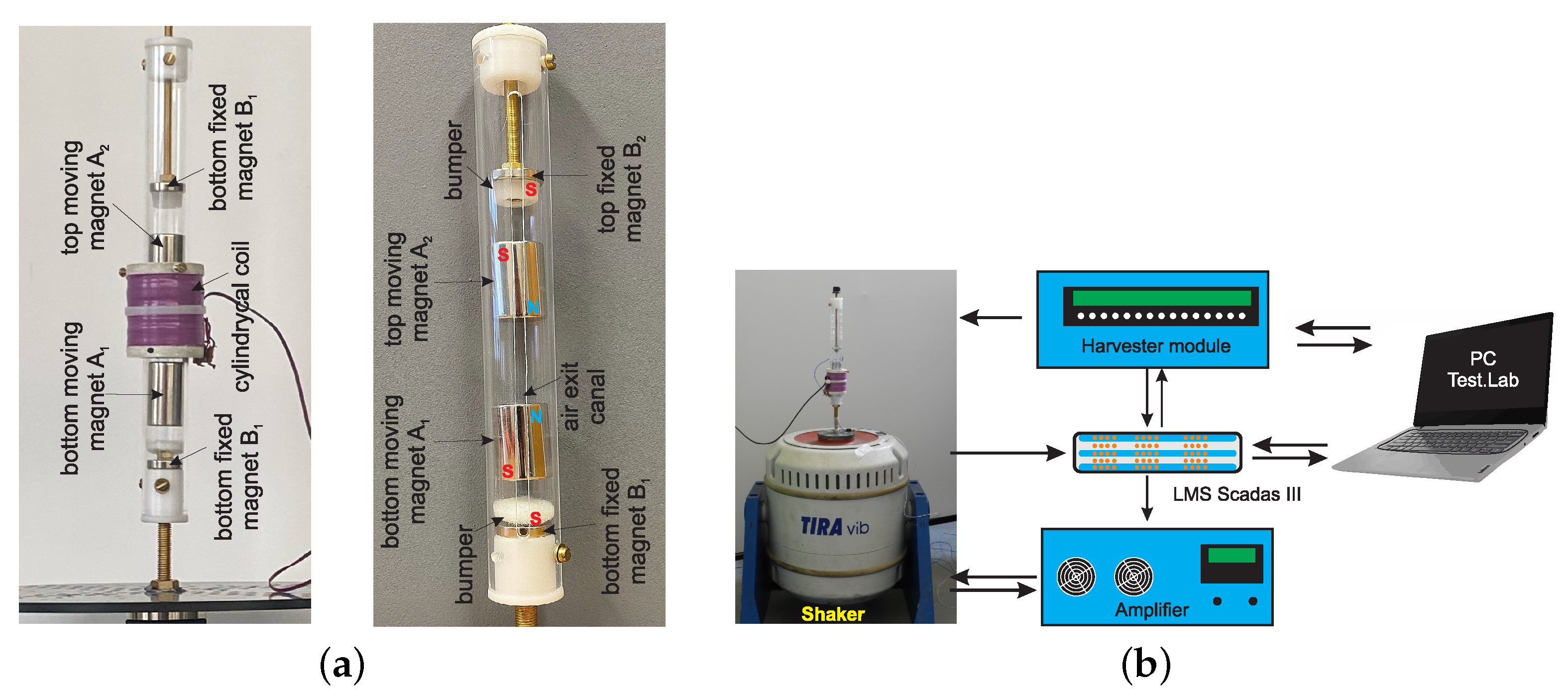
In this study, we focus on the development of an electromagnetic energy harvester with a wider operational frequency applicable for low-frequency vibrations. The rest of the paper is organized as follows. Section 2 is devoted to the modeling and prototyping of an electromagnetic harvester with a single coil and two levitating magnets. In this section, a new model of the magnetic suspension is proposed. Results and discussion are presented in Section 3, and conclusions are presented in Section 4.

2. Materials and Methods

2.1. Electromagnetic Harvester Device

A photograph of the proposed two-degrees-of-freedom (2DOF) harvester is shown in Figure 1a. In this harvester, resonance frequency and magnetic forces can be adjusted by grade, diameter, and shape of the permanent magnets and the distance (stroke) between the fixed magnets. The device consists of two neodymium magnets, $A_1$ and $A_2$, which move due to magnetic repulsion forces of the fixed (end) magnets, $B_1$ and $B_2$. Each of the moving magnets had a diameter of 20 mm and a length of 30 mm, while the end magnets had a diameter of 20 mm and a height of 5 mm. The properties of the harvester’s components are listed in

Table 1. Geometric parameters of the harvester device.

Parameter	Value
magnet moving diameter	20 (mm)
magnet moving height	30 (mm)
magnet fixed diameter	20 (mm)
magnet fixed height	5 (mm)
coil length	50 (mm)
coil inner diameter	22 (mm)
wire diameter	0.14 (mm)

. The magnets were made of materials such as NdFeB N38. The tube had an internal diameter of 21 mm. A small clearance between the tube and the moving magnets allowed the magnet to move freely. The clearance needed to be as small as possible to reduce the leakage rate of the magnetic field. A copper wire was wrapped around the portion of the tube and had 12,740 turns of coil. The coil resistance was estimated to be 1148 $\Omega$, which implied an average of 0.09 $\Omega$ per turn. The coil wire had a diameter of 0.14 mm.

Geometric and physical parameters of the magnetic and electrical harvester components are shown in Table 1.

All magnets were mounted in a non-magnetic PVC hollow cylinder equipped with a special air canal to eliminate air compression. The large height and small air gap of the floating magnets did not allow for rotation in the tube. The magnetic forces acting on the moving magnets were exerted by the lower and upper fixed magnets (end magnets). The tube was equipped with two bumpers to reduce the magnets’ collisions. These movable magnets could move inside the tube, and the end magnet forces acted as a magnetic spring. The opposite orientation of the magnets (poles) caused them to stabilize in an equilibrium position. The magnetic repulsive forces, which are described in Section 2.2 of this paper, were considered as linear damper and nonlinear spring forces induced by the movement of the magnets in the coil. The relative motion of the magnets inside the tube with respect to the fixed coil created a time-varying magnetic flux; therefore, an electromotive force was induced.

The harvester was connected to the harvester’s module and a computer with own software prepared in the C++ programming language to measure voltage induced from the harvester and magnet displacements as well as to provide load resistance (Figure 1b). The harvester module consists of a MicroDAQ module with OMAP L137 Texas Instruments processor and a conditioning device. The key role of the module is to measure the recovered voltage and control the load resistance. The analog outputs in the module made it possible to connect the device to the LMS Scadas data acquisition system. The harvester was mounted on the Tira shaker operated by the LMS system with Test.Lab. A special wireless sensor was attached to one of the magnets to measure magnet displacement. The sensor is based on a commercial ADXL354 accelerometer with added memory and a battery.

2.2. Magnetic Levitation Force

As far as magnetic levitation is concerned, the main characteristic of harvesters is magnetic levitation suspension. Therefore, in this section, the interaction between two moving magnets and two fixed magnets is described. The magnet’s orientation determines attractive or repulsive forces. The forces vary depending on the magnet’s separation distance, shape, diameter, and magnetization direction. The magnetic repulsive forces were induced in the experiment using a specially designed device (Figure 2a) and in the numerical simulation by FEM using the Comsol Multphysics software (https://www.comsol.com/, accessed on 16 May 2023) with progressively finer meshes to reach a higher precision (Figure 2b). There are many methods for computing magnetic forces in Comsol. The magnetic field was modeled using the magnetic field interface in the AC/DC module. The force is based on the surface integration of the Maxwell Stress Tensor, which is an integral computed over the exterior surfaces that are an arbitrary closed path. The geometry domain of magnets is selected for calculation. The movement of the magnet was modeled using the moving mesh interface. The material for the magnet used in the FEM simulation was neodymium N38, which was obtained from the materials module and solid mechanics interfaces selected in the coupling feature.

The measuring system (Figure 2a) was composed of a nonmagnetic tube with a compact sensor FX 292X-100A-0025-L for axial force measurement. Two cylindrical magnets were installed in the tube, and the distance between them could be adjusted with a vertical screw. A small sensor for magnetic force measurement was mounted inside the tube.

Magnetic forces between the moving magnets ($A_1$ or $A_2$) and the fixed magnets $B_1$ and $B_2$ are presented in Figure 3a. To estimate the magnetic force characteristics, each moving magnet was analyzed separately (without the second moving magnet). Then, the position of the magnet was changed, and the force was measured. Figure 3b shows the repulsive force between two moving magnets (between $A_1$ and $A_2$). The blue dots mark the experimental results, while the black line marks the FEM results. The experimental and numerical magnetic forces ($A_1$ and $A_2$) show high agreement. The magnetic force becomes too strong when the two moving magnets are too close to each other. The smaller the distance between the magnets is, the greater the difference between the FEM and experimental results becomes.

The proposed mathematical polynomial model (Equation (1)) is marked with a blue line. The red points and dashed vertical line mark the equilibrium position of both magnets. The equilibrium points (static position) are shifted away from the center point (point 0 in Figure 2b). It should be noted that the force between the moving magnets and two end magnets is different from that in the 1DOF harvester. For the classical 1DOF harvester, the magnetic restoring force resembles the Duffing characteristic [18,20]. However, in this case, the characteristic is different due to the orientation of the magnets (the moving magnet is attracted by one of the fixed magnets). The magnet $A_1$ is repelled by the fixed bottom magnet $B_1$ and attracted to the fixed top magnet (see Figure 2b).

The magneto-elastic forces as well as the magnetic field depend on the distance between the magnets. The relationship can be visualized in the form of magnetic field lines passing through the magnet along its direction of magnetization. The field strength relates to the density of the field lines in a certain area. The fixed magnet produces a field in its core and in its external surroundings. The magnetic field direction “flows” from one pole to the other. The magnetic norm and contour for two different magnet positions are shown in Figure 4a,b. The color scale refers to of the magnetic field density in (T). Each magnet yields a spatial distribution of the magnetic flux lines. These plots are useful for visualizing where the magnetic flux is stronger and how fast it decreases with distace from the magnet.

With two separated magnets, the magnetic flux is spread over the width of the structure, giving a weaker yet more homogeneous field. For simplicity, in the FEM model, the effect of rotation was omitted.

For the magnetic levitation harvester, the magnetic forces (called magneto-elastic) are crucial and decisive for the definition of resonant frequency. Magnetic force models are defined using the polynomial curve fitting approach with numerical and experimental findings. The mathematical model has been calculated using the MATLAB Curve Fitting Toolbox. It offers extensive fitting capability, including evaluating the goodness of fit using residuals and prediction bounds.

The magnetic forces between the moving and fixed magnets $F_{B_1{A}_1{B}_2}\left(x\right)$ and $F_{B_1{A}_2{B}_2}\left(x\right)$ were fitted to the experimental data, and a mathematical polynomial model was proposed,

$$F_{B_1{A}_1{B}_2}\left(x\right)=F_{B_1{A}_2{B}_2}\left(x\right)=p_1{x}^6+p_2{x}^5+p_3{x}^4+p_4{x}^3+p_5{x}^2+p_{6}x+p7,$$

(1)

where x is the moving magnet’s displacement ($x_1$ or $x_2$) and $p_1$–$p_7$ are the coefficients obtained from the curve-fitting technique. The magnetic force between the magnets $A_1$ and $A_2$ can be described by

$$F_{A_1{A}_2}(x_1,x_2)=1+k_{11}(x_1-x_2-0.1)+k_{22}{(x_1-x_2-0.1)}^5,$$

(2)

where $k_{11}$ and $k_{22}$ are the linear and nonlinear stiffness coefficients. All coefficients are listed in

Table 2. Parameters of the 2DOF harvester and the nonlinear coefficients of the magnetic spring.

Parameter	Value	Parameter	Value
m	0.09 (kg)	p${}_1$	1.098 $\times {10}^9$
c	0.07 (Ns/m)	p${}_2$	1.106 $\times {10}^4$
k${}_{11}$	−0.000039577 (N/m)	p${}_3$	−7.762 $\times {10}^5$
k${}_{22}$	−99,042,000 (N/m)	p${}_4$	−38.85
L	1.46 (H)	p${}_5$	2170
R	1000 ($\Omega$)	p${}_6$	0.03027
${\alpha }_1$	30 (N/A)	p${}_7$	−0.1523
${\alpha }_2$	30 (N/A)

. The fit goodness of the proposed models is described by the R-square parameter, having a value of about 0.97, which indicates that a greater proportion of variance is accounted for by the model.

2.3. Modeling

The proposed theoretical nonlinear electromagnetic harvester can be simplified to a 2DOF lumped-parameter model connected by magnetic springs, as shown in Figure 5. Both levitating magnets move axially on the tube when the harvester is excited by the shaker. The mass of the suspended moving magnets is identical: $m_1$ = $m_2$ = m. In the harvester, there are three damping sources: friction from contact of the magnet with the tube, air damping, and electromagnetic damping. Because both magnets are identical, the mechanical damping describing the total damping of both magnets is also the same and denoted by c.

The model consists of three subsystems, two of which are mechanical and one electromagnetic. Based on Newton’s second law, the system dynamics can be described by time-dependent coupled nonlinear differential equations, two of which describe the dynamics of the magnets, and one that represents the electrical circuit output connected to the external resistive load:

$$m{\ddot{x}}_1+c{\dot{x}}_1+F_{B_1{A}_1{B}_2}\left(x_1\right)-F_{A_1{A}_2}(x_1,x_2)+{\alpha }_1\dot{i}=m({\ddot{x}}_s+g),$$

(3)

$$m{\ddot{x}}_2+c{\dot{x}}_2-F_{B_1{A}_2{B}_2}\left(x_2\right)+F_{A_1{A}_2}(x_1,x_2)+{\alpha }_2\dot{i}=m({\ddot{x}}_s+g),$$

(4)

$$L\dot{i}+Ri={\alpha }_1{\dot{x}}_1+{\alpha }_2{\dot{x}}_2.$$

(5)

The coordinates $x_1$ = $X_1$− $x_s$ and $x_2$ = $X_2$− $x_s$ denote the relative magnet’s displacements, where $x_s$ is the shaker’s displacement. The i is the induced current in the coil, from which the recovered energy can be easily estimated (P = $i^{2}R$). The magnet’s positions are measured from the equilibrium points of both magnets relative to the coil’s center. Parameters ${\alpha }_1$ and ${\alpha }_2$ are the electromechanical coupling coefficients that characterize interaction between mechanical and electrical subsystems. These parameters can be estimated based on a geometry magnet-coil system or by simply testing a magnet moving through a coil with known speed [18]. The coil with a resistance $R_C$ and an inductance L is connected to the resistor with a load resistance $R_L$ (the total resistance is R = $R_L$ + $R_C$). The magneto-elastic forces described in Section 2.2 are $F_{B_1{A}_1{B}_2}\left(x_1\right)$, $F_{B_1{A}_2{B}_2}\left(x_2\right)$, and $F_{A_1{A}_2}(x_1,x_2)$. The moving magnets generate a complex current–time signal when the system is excited. Harmonic excitation is generated by the shaker and LMS software (https://elearningindustry.com/directory/software-categories/learning-management-systems, accessed on 16 May 2023), by a harmonic force ${\ddot{x}}_s$ = Acos$\omega t$, where $\omega$ and A are the frequency and amplitude of excitation, respectively.

A detailed analysis of Equation (5) shows that the induced voltage (and current) for a given electrical load depends on the levitating magnets’ velocities and the electromechanical coupling coefficients; hence, the mechanical and electromagnetic subsystems are strongly coupled. Generally, the electromechanical coupling depends on the magnet’s position in the coil, with the highest values obtained close to the coil’s end. However, Kecik et al. [18] showed that the electromechanical coupling could be treated as a constant if selected properly.

3. Results and Discussion

In order to validate the proposed 2DOF harvester model in relation to the experimental results, the physical parameters of the device must be quantified. Most of them are easily measurable and are listed in Table 2. The electromechanical coupling $\alpha$ is measured using a quasi-static test of a single magnet moving through the coil [18]. The damping coefficients are determined by the parameter identification method based on experimental frequency response data (comparing time histories from numerical simulation and experiment; see paper [24]).

Three differential Equations (3)–(5) were numerically solved using the path-following (continuation) method in the Auto-07p software (https://sourceforge.net/projects/auto-07p/, accessed on 16 May 2023) [30] in order to predict the magnets’ responses and output current over a range of frequencies for different acceleration levels. The continuation method is used to study bifurcations, such as equilibria, stability, periodic and homoclinic orbits, and boundary-value problems. More information about this method can be found in [31].

3.1. Simulation Results and Model Validation

The validation of the numerical model is an important stage in ensuring the reliability of the results obtained. To that end, numerical results must be compared with experimental data. Figure 6 shows an example of comparison of the numerical (blue line) and experimental (orange line with circles) frequency response qualitative curves for the bottom magnet (Figure 6a) and induced current (Figure 6b), respectively. The experimental curves were obtained by testing the harvester prototype on the dynamic workbench described in Section 2.1. The frequency response was measured for a sinusoidal excitation on the shaker with an amplitude of A = 0.6 g, where g is the gravitational acceleration. The test was made for forward or backward frequency sweeps with a step 0.5 of Hz and an interval of 5 s.

Generally, the numerical model successfully predicted the nonlinear frequency response curves, and it is observed that the experimental and simulation results are consistent. The presence of two resonance peaks is confirmed, although the experimental peak values are considerably lower.

These differences could be explained by the estimates of damping and the assumptions of constant magnet friction and fixed electromechanical coupling. These assumptions are responsible for errors in the calculation of the numerical resonance curves. Moreover, the resonant frequencies of the experimental results are slightly shifted to the left compared to their numerical equivalents (a detuning phenomenon). This effect may be related to the small rotations of the magnet and the contact of the magnet with the bumper.

3.2. Frequency Response Curve

In the linear harvester, the magnitude of excitation does not affect the resonance bandwidth. However, in the nonlinear harvester, excitation has a great impact on response. Therefore, frequency response analysis is one of the most important analyses in nonlinear systems, because it shows the resonance frequencies of a system and the relative peak amplitude. The main aim of the frequency response is to obtain information about the magnet oscillation level and to obtain the frequencies where the recovered current (and power) is highest. In this subsection, the 2DOF nonlinear harvester is investigated using different excitation accelerations, e.g., from 0.2÷1 g. The maximum (MAX(x${}_1$), MAX(x${}_2$)) and minimum (MIN(x${}_1$), MIN(x${}_2$)) responses of both magnets and the output maximum current (MAX(i)) are analyzed. The displacements of magnets are measured according to the coordinate system from Figure 5.

In Figure 7, the maximum and minimum displacements of the top (Figure 7a) and bottom (Figure 7b) magnets, as well as the maximum recovered current (Figure 7c), are shown. These diagrams were plotted by sweeping the frequency $\omega$ from 20 rad/s to 140 rad/s, for different amplitudes: 0.2 g (black line), 0.6 g (blue line), and 1 g (green line). The dashed line denotes the static position (equilibrium) of both magnets, while the continuous line indicates the stable solution (stable fixed point). The red line between the fold (saddle-node) bifurcation points $FB$ denotes the unstable solution (unstable fixed point). Fold bifurcations occur when two equilibria come together and disappear [32].

It can be noted that the main (first) resonance is observed for $\omega$ ≈ 60 rad/s, while the second one is for $\omega$ ≈ 120 rad/s. It should be noted that the maximal and minimal displacements are not symmetric. An increase in the amplitude of excitation causes an increase in the magnet oscillations, and the hardening effect can be observed. In the first resonance, the hardening effect characterizes two stable and one unstable solution, occurring for A = 1 g (green line). The multistability is caused by a fold bifurcation ($FB$) where the stable and unstable branches meet. The peak-to-peak top and bottom magnets’ output responses are quite similar and amount to 0.022 m (for A = 1 g). Interestingly, the resonance of the recovered current shows two peaks close to the frequencies of $\omega$ ≈ 60 rad/s and 70 rad/s (Figure 7c). These peaks are the result of the dynamic vibration absorption effect. The bottom magnet, for some parameters, causes vibration reduction of the top magnet (region between both peaks). This phenomenon exists in a 2DOF system. Between the two similar peaks, the recovered current decreases from 28 mA (for $\omega$ = 58 rad/s) to 14 mA (for $\omega$ = 60 rad/s). This means that the instantaneous power changes from 0.78 W to 0.2 W.

The second resonance exhibits a multistability behavior, which could already be observed for 0.6 g. This resonance is characteristic of lower magnet oscillations, and the recovered current is about 0.01 mA (0.1 W). However, the peak-to-peak top and bottom magnet response is about 0.02 m (for A = 1 g). It should be noted that the first resonance has a wider frequency bandwidth. Interestingly, close to the second resonance, for a frequency of $\omega$ ≈ 120 rad/s, a strong dynamic absorption of the top magnet occurs. For a frequency of $\omega$ ≈ 110 rad/s, the oscillation of the bottom magnet disappears.

In Figure 7d, the multistability regions with two stable and one unstable solution in the first and second resonances are plotted (orange region). An analysis of both regions reveals that the multistability region in the second resonance is larger. When the excitation amplitude increases, the multistability tongues expand. However, in the first resonance, an unstable region appears (pink region in Figure 7d), caused by the Neimark–Sacker ($NS$) bifurcation. This bifurcation is interesting because it causes the equilibrium to lose stability.

The time histories of the bottom and top magnets (black lines) at $\omega$ = 60 rad/s and A = 0.6 g are shown and compared in Figure 8a. Both time responses are similar and have two harmonic components.

For the top and bottom magnets, the peak-to-peak values are comparable and equal to approximately 0.008 m. The signal of the induced current (red line) is clearly periodic. The peak-to-peak induced voltage equals 0.024 A.

Figure 8b shows the time histories of the induced current in the first and second resonances for an amplitude of A = 1 g. It can be observed that the peak-to-peak induced current decreased from 0.027 A to 0.015 A (comparing both resonances).

3.3. Influence of Amplitude Excitation

To determine the influence of the excitation amplitude on the system dynamics and nonlinear resonance, the excitation frequency $\omega$ was fixed, and then magnet responses were computed versus the bifurcation parameter A. Two fixed frequency values were applied: $\omega$ = 60 rad/s (blue line) and $\omega$ = 120 rad/s (black line). The two displacements were analyzed for each magnet ($MAX$ and $MIN$). This means that the magnet oscillates between both lines. It is similar to the envelope of time series. For a certain range of parameters, the lines intersect, which means that more than one solution exists.

Figure 9a shows the bifurcation diagram for the top magnet. Figure 9b,c presents the bifurcation diagrams for the bottom magnet and induced current, respectively.

All bifurcation diagrams correspond to each other and provide similar results. The bifurcation branches computed begin from the equilibrium point, which causes an increase in A. An analysis of the results obtained for $\omega$ = 60 rad/s shows four possible scenarios: (1) one stable solution, if the amplitude ranges from A = 0 m/s${}^2$ to the $FB2$ point, and from the $NS2$ point (A = 12.5 m/s${}^2$) to A = 20 m/s${}^2$; (2) two stable and one unstable solution between the bifurcation points $FB2$ and $NS1$; (3) two unstable and one stable solution between $NS1$ and $FB1$; and (4) a small region with only one unstable solution between $FB1$ and $NS2$ (pink region). The unstable periodic time courses in this region are shown in Figure 9. The coexistence of the stable solutions (branches) results from the fold bifurcation points that change stability from stable to unstable ($FB1$) and from unstable to stable ($FB2$) during turning, and the coexistence of the solutions depends on the initial conditions.

For a frequency of $\omega$ = 120 rad/s (black line), only two bifurcation scenarios are observed. The first is one stable branch between 0 and $FB2$ and between $FB1$ and 20 rad/s. The second is two stable and one unstable solution occurring between the $FB2$ and $FB1$ bifurcation points. It should be noted that in the case with two stable solutions, one of them has a higher energy output. For example, for a frequency of $\omega$ = 120 rad/s and an amplitude of A = 10 m/s${}^2$, the recovered energy from the bottom branch is about 0.016 W and that from the top branch is 0.064 W. The behavior of the two frequencies is different in the studied cases. In the first resonance, unstable solutions caused by NS bifurcations appear in the same branch. The unstable solution appears between the $NS1$ and $NS2$ bifurcation points.

3.4. Influence of Electromechanical Coupling

The electromechanical coupling coefficient ($\alpha$) measures the efficiency of converting input mechanical energy into electrical energy. It can be changed by modifying the magnet–coil design, using specially designed magnets with separators, adding additional magnets, or modifying the resonance behavior [33]. An increase in the coupling coefficient also causes greater damping in the harvester system, which makes this parameter crucial for energy harvesting. In strong nonlinear systems, especially those with many degrees of freedom and many electromechanical couplings, their impact is difficult to predict.

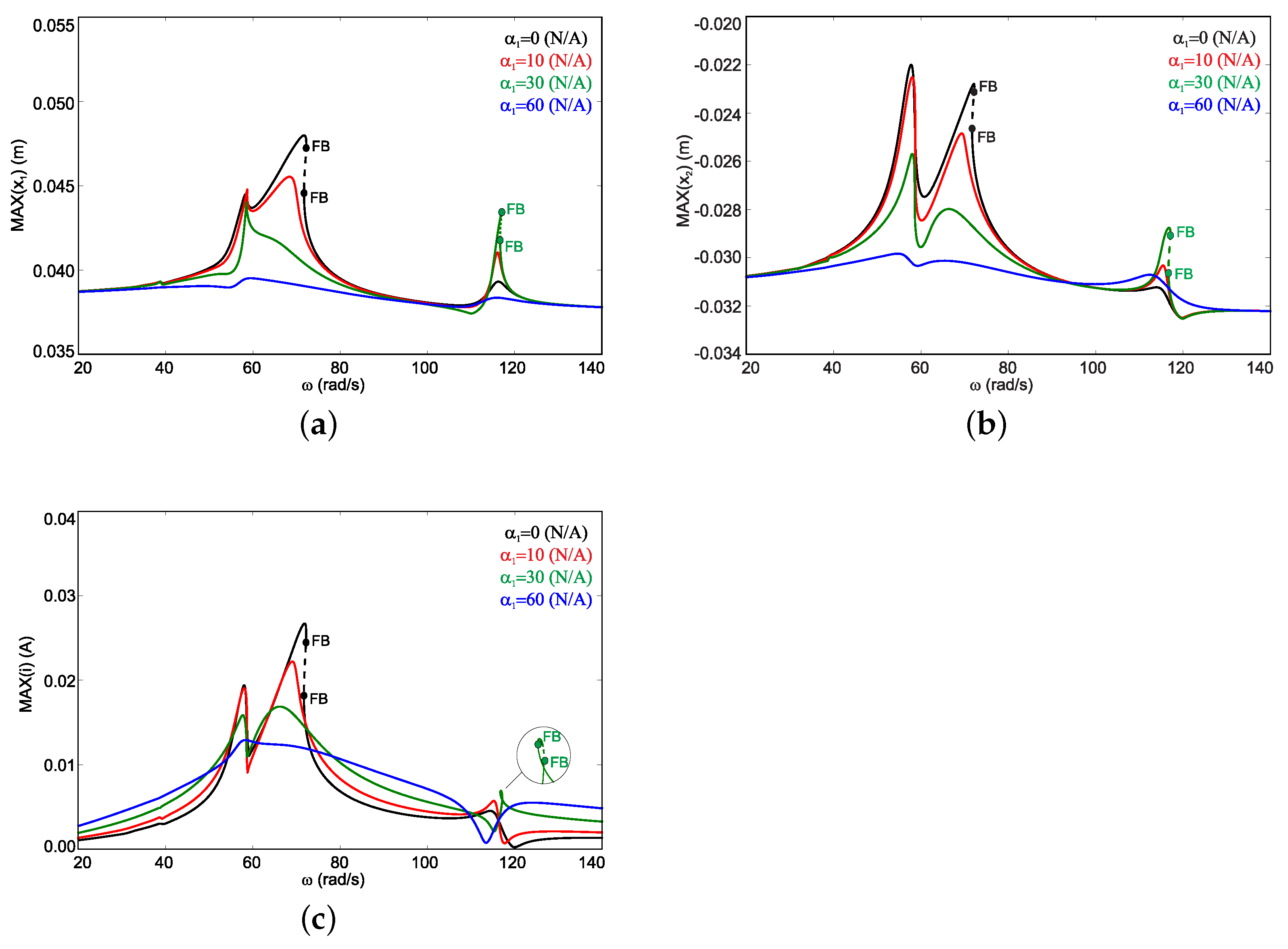
A comparison of the resonance curves for different electromechanical couplings is given in Figure 10 and Figure 11. The resonance curves were obtained by path following of the periodic solutions, starting from $\omega$ = 20 rad/s. The circles denote the bifurcation fold points. Two strategies for electromechanical coupling analysis were applied. First, the electromechanical coupling between the top magnet and the coil (${\alpha }_2$) was modified, and the fixed value of the bottom magnet’s electromechanical coupling was assumed (${\alpha }_1$ = 30 N/A). For ${\alpha }_2$ = 0 N/A (no coupling between the mechanical and electrical subsystems − black line), both magnets exhibit the highest oscillation, and the main nonlinear resonance (two peaks with a hardening behavior) is observed close to the frequency $\omega$ = 60 ÷ 80 rad/s. For this case, the recovered current is the highest and amounts to about $i_{MAX}$ = 0.038 A (Figure 10c).

An increase in ${\alpha }_2$ to 10 N/A causes a reduction in the oscillation of both magnets in the first resonance (red line). When both electromechanical couplings are identical (green line), then the hardening effect occurs in the second resonance. For ${\alpha }_2$ = 60 N/A (blue line), the hardening effect is reduced in both resonances, and no bifurcation points occur. The obtained resonance curves are similar to those of the linear system [34] (the bending effect is not observed). Interestingly, the peak in the second resonance is the lowest for ${\alpha }_2$ = 0 N/A, but higher for ${\alpha }_2$ = 30 N/A and ${\alpha }_2$ = 60 N/A. This means that the higher electromechanical coupling between the bottom magnet and the coil improved recovered current near the second resonance.

The second strategy is similar: a fixed electromechanical coupling between the top magnet and the coil was assumed (${\alpha }_2$ = 30 N/A), and the parameter ${\alpha }_1$ was changed. Figure 11 shows the influence of ${\alpha }_1$ on the harvester response and induced current. It can be observed that the ${\alpha }_1$ parameter plays a similar role to ${\alpha }_2$. An increase in ${\alpha }_1$ causes the magnet amplitude to decrease and the main nonlinear resonance to be reduced. However, the in the second resonance, the recovered current is higher for an ${\alpha }_1$ of 30 N/A and 60 N/A.

An analysis of the obtained curves in Figure 10 and Figure 11 reveals that the electromechanical coupling influences the foldover effect that is responsible for the bending of the resonance curve in an amplitude versus frequency plot. The effect is characterized by two stable and one unstable solution. In Figure 12a, a two-parameter continuation was used to obtain the foldover region in the main resonance. First, it was assumed that ${\alpha }_1$ = 0 N/A and that ${\alpha }_2$ and $\omega$ were changed (dark orange color). Second, ${\alpha }_2$ = 0 N/A, and ${\alpha }_1$ and $\omega$ were changed (light region). The continuation started at the $FB$ point (black point close to $\omega$ ≈ 77 rad/s) and followed the path to its subsequent positions (black borderline). The direction of path-following continuation was marked with arrows. The results showed that the critical values of the electromechanical couplings for foldover reduction were ${\alpha }_{2CR}$ = 12 N/A and ${\alpha }_{1CR}$ = 4 N/A. It should be noted that the foldover effect is more sensitive to the ${\alpha }_1$ parameter, which is in agreement with the resonance curves in Figure 11.

Figure 12b shows the two-parameter continuation of the foldover effect occurring in the main resonance. The continuation began at the point where ${\alpha }_1$ = ${\alpha }_2$ = 30 N/A. For this case, both electromechanical couplings affect the foldover region in the same way. Interestingly, for some frequencies, the foldover regions overlap. This means that both couplings can be used to control the resonance curve bend.

The results of the numerical simulations indicate that the electromechanical coupling parameters ${\alpha }_1$ and ${\alpha }_2$ have a significant impact on the harvester dynamics and the recovered current. In addition to this, the electromechanical coupling parameters can be used for multistability control.

4. Conclusions

This study has investigated a two-degrees-of-freedom electromechanical vibration energy harvester. The numerical simulations and experimental prototype validation have confirmed the theoretical predictions. Magnetic suspension forces were estimated experimentally, and mathematical models were proposed.

The two resonances were detected and experimentally verified. In the resonance curves, the effect of dynamic vibration absorption was noticeable. A small shift between the numerical and experimental resonance peaks was observed. The frequency analysis showed the hardening effect for higher amplitudes of excitation. Inside the first resonance, an unstable region caused by the Neimark–Sacker (torus) bifurcation was observed. The bifurcation analysis showed the presence of multi-solution regions. Apart from the standard region with two stable and one unstable solution (hardening effect), two unstable and one stable solution were observed. The energy harvester benefits from the multistability because both the output response amplitude and the recovered power can be higher.

The analysis of the electromechanical couplings showed that these parameters acted as damping, generally reducing the main resonance. However, in the second resonance, an increase in the electromechanical coupling improved the induced current. Therefore, it can be concluded that a proper configuration of both couplings could increase the effectiveness of energy harvesting. This means that electromechanical couplings can be used to control harvester dynamics as well as energy harvesting.

In the future, the multistability and electromechanical coupling modification will be controlled by design of the magnet–coil system and also by using additional magnets close to the coil.

5. Patent

The result of the work is a Polish patent: “Device for measuring magnetic forces, especially between cylindrical magnets”, no. P.438043 (Figure 2a).