Adaptive-Dynamic-Programming-Based Robust Control for a Quadrotor UAV with External Disturbances and Parameter Uncertainties

Abstract

Thiswork addresses the trajectory-tracking-control problem for a quadrotor unmanned aerial vehicle with external disturbances and parameter uncertainties. A novel adaptive-dynamic-programming-based robust control method is proposed to eliminate the effects of lumped uncertainties (including external disturbances and parameter uncertainties) and to ensure the approximate optimal control performance. Its novelty lies in that two radial basis function neural network observers with fixed-time convergence properties were first established to reconstruct the lumped uncertainties. Notably, they tune only the scalar parameters online and have low computational complexities. Subsequently, two actor–critic neural networks were designed to approximate the optimal cost functions and control policies for the nominal system. In this design, two new actor–critic neural network weight update laws are proposed to eliminate the persistent excitation condition. Then, two adaptive-dynamic-programming-based robust control laws were obtained by integrating the observer reconstruction information and the nominal control policies. The uniformly ultimately bounded stability of the closed-loop tracking control systems was ensured using the Lyapunov methodology. Finally, numerical results are shown to verify the effectiveness and superiority of the proposed control scheme.

1. Introduction

In recent years, unmanned aerial vehicles (UAVs) have attracted significant research interest on account of their wide range of applications in both the civilian and military fields, such as agricultural production, logistics and distribution, urban management, border blockade prevention, reconnaissance, surveillance, etc. [1,2,3,4,5]. Compared with other flight vehicles, a quadrotor UAV has many significant advantages, including a simple structure, vertical take-off and landing, a low manufacturing cost, and so on [6]. However, the quadrotor UAV flight control system is an underactuated system, and its dynamic model possesses the characteristics of nonlinearity and a strong coupling of the translational and rotational dynamics. Moreover, it is very sensitive to disturbances, including external gust disturbances, aerodynamic effects, model uncertainties, and so on. Considering the trajectory tracking control of a quadrotor UAV as the basis for the previously mentioned applications, a series of extensive studies has been undertaken on this subject. For practical applications, linear control schemes have been adopted to linearize the complex dynamic model to ensure the basic operation of a quadrotor UAV, such as proportional–integral–derivative (PID) control [7] and linear quadratic regulator (LQR) control [8]. However, the linear model can cause performance degradations when performing complex tasks and when in unknown environments. In order to improve the tracking performance, various nonlinear control strategies have been further studied, including sliding mode control [9,10], backstepping control [11], adaptive control [12], and so on. However, the control schemes mentioned above only focus on the stability of the system and do not consider the control cost. Since mobile vehicles can carry limited energy equipment, it is necessary to consider the control cost and energy optimization [13,14]. Therefore, it is of great significance to design a tracking control scheme that can not only stabilize the quadrotor UAV flight control system, but also minimize its control cost.

Adaptive dynamic programming (ADP) is an optimization-theory-based control method and achieves a balance between the control cost and control performance by adaptively adjusting the control policy. As an effective method for solving the optimal control problems of nonlinear systems, it has received much attention in its related fields. Werbos et al. [15] first proposed a heuristic dynamic programming algorithm based on reinforcement learning and designed a preliminary online learning control framework. Vamvoudakis et al. [16] proposed an online algorithm based on actor–critic neural networks (AC NNs) to learn the optimal control solutions for nonlinear systems of known dynamics with an infinite horizon cost. The AC NNs were used to approximate the control policy and cost function, respectively. Kamalapurkar et al. [17] investigated an ADP-based optimal tracking problem for nonlinear systems. Wang et al. [18] solved the robust stabilization problem via adaptive-critic-based techniques. Wen et al. [19] introduced a new optimized backstepping control method based on ADP and backstepping technologies, which solved the tracking control problem of strict feedback systems. Furthermore, ADP technology has also been extensively researched in fault-tolerant control [20], zero-sum games [21], multi-agent systems [22], etc. However, most of the existing weight update laws are required to satisfy persistent excitation (PE) conditions. It is worth mentioning that some scholars have performed successive studies to avoid the use of PE conditions and make ADP technology easier to implement in practical engineering. In [23,24], the experience replay technique was utilized to overcome the PE condition for weight convergence. Dong et al. [25] proposed a simplified online learning strategy, which removed the PE conditions via the concurrent learning method. Liu et al. [26] designed a novel weight update law by utilizing adaptive technology, which removed the PE condition. Unfortunately, most of the existing methods still rely on real data. Thus, how to effectively avoid the use of PE conditions is still an open problem.

Meanwhile, uncertainties can seriously degrade the performance of a quadrotor UAV flight control system. Uncertainties usually have time-varying characteristics, and the ADP technique lacks the ability to tackle time-varying signals [26,27]. Thus, it alone cannot be utilized to achieve high-quality control of quadrotor UAVs. Therefore, integrating the uncertainty attenuation technique with the ADP technique is of great significance in solving the control problems of quadrotor UAVs. In recent years, due to their strong fitting ability, neural networks (NNs) have provided some promising approaches to the uncertainty attenuation problem in practical systems such as quadrotor UAVs [28,29,30,31,32]. Zhao et al. [30] proposed an NN-based adaptive control scheme for the unknown and continuous dynamics of quadrotor UAVs, which cannot achieve fast convergence characteristics. To improve the convergence speed of the control system, some scholars have integrated finite-time control techniques with NN-based techniques. Wang et al. [31] proposed a control scheme based on a finite-time multivariate NN interference observer for helicopter systems. Liu et al. [32] proposed an adaptive NN-learning-based control scheme with finite-time convergence characteristics for the quadrotor UAV fault-tolerant control problem. However, the performance of the finite-time control techniques depends heavily on the initial state errors or observation errors, which limits the scope of their application in quadrotor UAVs. Therefore, combining NN-based techniques with fixed-time techniques for application in a quadrotor UAV control system requires further research. In addition, NN units commonly directly approximate the uncertainties in the above-mentioned studies, which leads to a large computational load and parameter explosion.

Motivated by the aforementioned significant research, this paper investigated the control scheme of a quadrotor UAV under external disturbances and parameter uncertainties. The investigation focused on tracking control by integrating the NN-based observer technique with the ADP-based control technique, ensuring that the resulting control laws demonstrate both robust and approximately optimal characteristics. The main contributions are outlined below:

(1)

Two fixed-time NN-based observers (FTNNOBs) were developed to compensate the control inputs of quadrotor UAV, which can estimate external disturbances and parameter uncertainties in a fixed time. Different from the traditional NN approximators designed in [33,34,35], the FTNNOBs only need to adjust the scalar parameters rather than the weight vectors or matrices. They provided a simple structure and inexpensive computation.

(2)

A novel ADP-based robust control scheme is proposed by combining the ADP technique with the estimated information from FTNNOBs, which improves the tracking control accuracy and optimizes the control cost consumption. Different from the existing weight update laws of AC NNs [16,25], two novel weight update laws were introduced in this work. They not only have a simple structure, but are also independent of the PE condition. Moreover, two auxiliary terms related to the system states were introduced to improve the data utilization efficiency of the AC NNs and make the training results more effective.

The rest of the paper is organized as follows. Section 2 introduces the dynamics model of a quadrotor UAV and derives the position and attitude error systems. Section 3 describes the design process of the ADP-based robust control scheme and the stability analysis of the overall closed-loop system. Section 4 introduces the simulation results. Section 5 presents the conclusions of this paper.

Notations 1. 

$∥·∥$ is utilized for the Euclidean norm of vectors and matrices. ${\lambda }_{\min }(·)$ and ${\lambda }_{\max }(·)$ represent the minimum or maximum eigenvalues of symmetric matrices, respectively. For any $\mathit{x}={[x_1,x_2,\cdots ,x_n]}^{\mathrm{T}}$, we define ${\mathrm{sig}}^{\eta }\left(\mathit{x}\right)={[{\left|x_1\right|}^{\eta }\mathrm{sgn}\left(x_1\right),\cdots ,{\left|x_n\right|}^{\eta }\mathrm{sgn}\left(x_n\right)]}^{\mathrm{T}}$, where $\eta \in {\mathcal{R}}^{+}$, $\mathrm{sgn}(·)$ denotes the sign function. ${\mathit{I}}_n$ represents an identity matrix of size n.

2. Model Description and Transformation

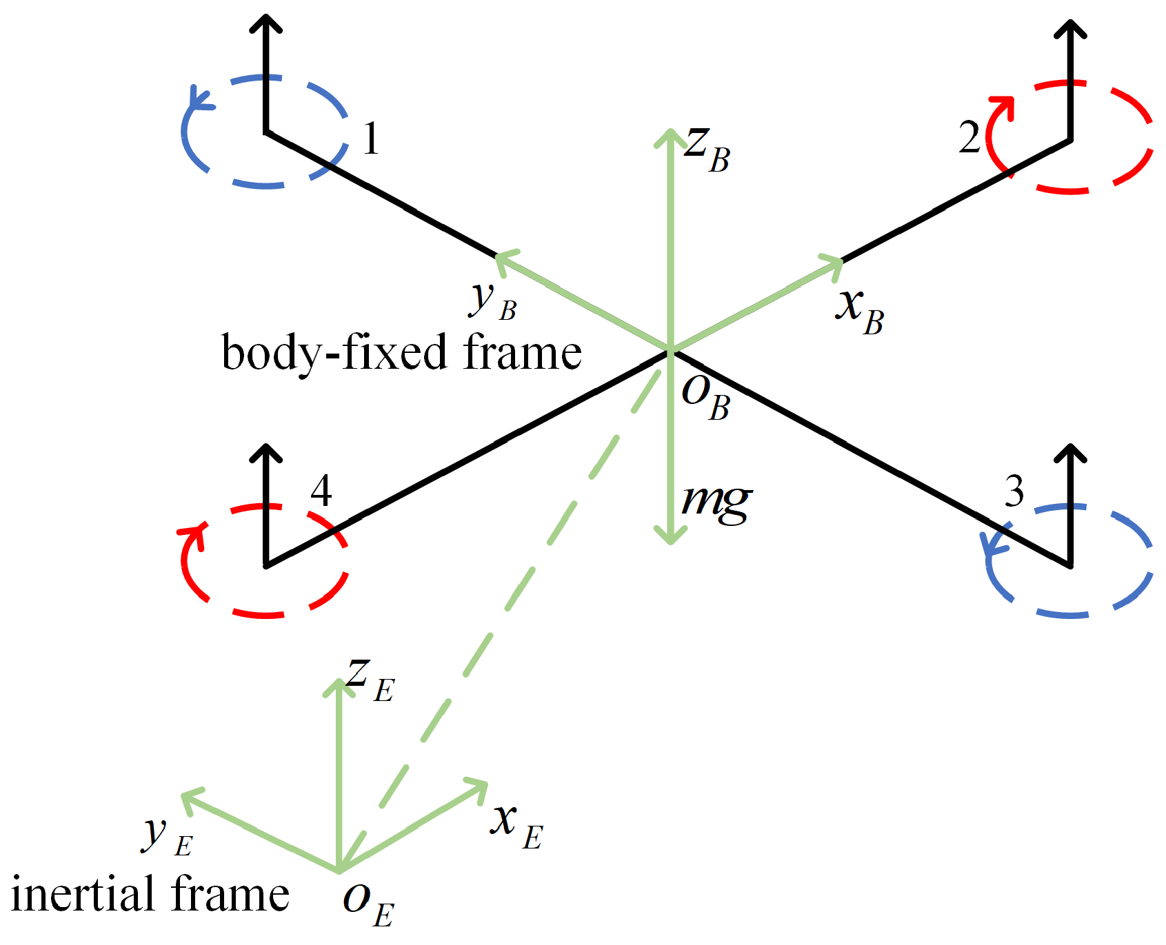
2.1. Dynamics Model

The mechanical structure of a quadrotor UAV and the coordinate reference system are shown in Figure 1. ${\mathit{\varsigma }}_E\left\{{\mathit{o}}_E{\mathit{x}}_E{\mathit{y}}_E{\mathit{z}}_E\right\}$ is the Earth-fixed inertial frame. ${\mathit{\varsigma }}_B\left\{{\mathit{o}}_B{\mathit{x}}_B{\mathit{y}}_B{\mathit{z}}_B\right\}$ denotes the body-fixed frame. In the frame ${\mathit{\varsigma }}_E$, $\mathit{\zeta }={[x,y,z]}^{\mathrm{T}}\in {\mathcal{R}}^3$ presents the position state vector. $\mathbf{\Theta }={[\varphi ,\theta ,\psi ]}^{\mathrm{T}}\in {\mathcal{R}}^3$ is the Euler angle vector, in which $\varphi ,\theta$ and $\psi$ denote the roll, pitch, and yaw angles. $\mathit{\eta }={[u,v,w]}^{\mathrm{T}}\in {\mathcal{R}}^3$ and $\mathbf{\Omega }={[p,q,r]}^{\mathrm{T}}\in {\mathcal{R}}^3$ are the linear and angular velocity vectors under the frame ${\mathit{\varsigma }}_B$, respectively. Furthermore, the kinematic transformation relationships of the quadrotor UAV between the frame ${\mathit{\varsigma }}_E$ and ${\mathit{\varsigma }}_B$ are introduced as [32]:

$$\begin{array}{c}\hfill \dot{\mathit{\zeta }}={\mathit{R}}_B^E\mathit{\eta },\dot{\mathbf{\Theta }}={\mathbf{\Phi }}_B^E\mathbf{\Omega },\end{array}$$

(1)

where the transformation matrices ${\mathit{R}}_B^E$ and ${\mathbf{\Phi }}_B^E$ from the frame ${\mathit{\varsigma }}_B$ to ${\mathit{\varsigma }}_E$ can be expressed as

$$\begin{array}{c}\hfill \begin{array}{c}\hfill {\mathit{R}}_B^E=\left[\begin{array}{ccc}C\theta C\psi & S\varphi S\theta C\psi -C\varphi S\psi & C\varphi S\theta C\psi +S\varphi S\psi \\ C\theta S\psi & S\varphi S\theta S\psi +C\varphi S\psi & C\varphi S\theta S\psi -S\varphi S\psi \\ -S\theta & S\varphi C\theta & C\varphi C\theta \end{array}\right],\end{array}\end{array}$$

$$\begin{array}{c}\hfill {\mathbf{\Phi }}_B^E=\left[\begin{array}{ccc}1& S\varphi T\theta & C\varphi T\theta \\ 0& C\varphi & -S\varphi \\ 0& S\varphi /C\theta & C\varphi /C\theta \end{array}\right],\end{array}$$

with $S·,C·$ and $T·$ denoting $\sin (·),\cos (·)$ and $\tan (·)$, respectively. The dynamical model [36,37] with respect to the frame ${\mathit{\varsigma }}_B$ can be established as

$$\begin{array}{c}\hfill \begin{array}{c}m\dot{\mathit{\eta }}=-{\mathbf{\Omega }}_{\times }m\mathit{\eta }-{\mathit{F}}_f+{\mathit{F}}_g+{\mathit{U}}_f+{\mathit{D}}_f,\\ \mathit{J}\dot{\mathbf{\Omega }}=-{\mathbf{\Omega }}_{\times }\mathit{J}\mathbf{\Omega }-{\mathit{M}}_t+{\mathit{G}}_a+{\mathit{U}}_t+{\mathit{D}}_t,\end{array}\end{array}$$

(2)

where m is the total mass of the quadrotor UAV. $\mathit{J}=\mathrm{diag}\left\{J_x,J_y,J_z\right\}\in {\mathcal{R}}^{3\times 3}$ represents the moments of inertia. ${\mathit{F}}_f={[k_{1}u,k_{2}v,k_{3}w]}^{\mathrm{T}}\in {\mathcal{R}}^3$ and ${\mathit{M}}_t={[k_{4}p,k_{5}q,k_{6}r]}^{\mathrm{T}}\in {\mathcal{R}}^3$ represent aerodynamic friction vectors with $k_1,k_2,\cdots ,k_6$ being the aerodynamic friction coefficients. ${\mathit{U}}_f={[0,0,f]}^{\mathrm{T}}\in {\mathcal{R}}^3$ is the total thrust vector, and ${\mathit{U}}_t={[U_{t1},U_{t2},U_{t3}]}^{\mathrm{T}}\in {\mathcal{R}}^3$ denotes the control torque vector. ${\mathit{D}}_f={[D_{f1},D_{f2},D_{f3}]}^{\mathrm{T}}\in {\mathcal{R}}^3$ and ${\mathit{D}}_t={[D_{t1},D_{t2},D_{t3}]}^{\mathrm{T}}\in {\mathcal{R}}^3$ denote the external disturbance vectors of the quadrotor UAV.

${\mathit{F}}_g={\left({\mathit{R}}_B^E\right)}^{-1}{[0,0,-mg]}^{\mathrm{T}}\in {\mathcal{R}}^3$ denotes the gravity vector with g being the gravity coefficient. ${\mathit{G}}_a={[J_{r}q\overline{\omega },-J_{r}p\overline{\omega },0]}^{\mathrm{T}}\in {\mathcal{R}}^3$ represents the gyroscopic moment vector, where $J_r$ is the inertia of each motor, and $\overline{\omega }={\omega }_1-{\omega }_2+{\omega }_3-{\omega }_4$ is the total residual rotor speed. Note that the inaccessibility of the rotor speed, ${\mathit{G}}_a$ is considered as an additional disturbance during the control design [38]. In addition, ${(·)}_{\times }$ denotes the skew-symmetric matrix satisfying

$$\begin{array}{c}\hfill {\mathit{x}}_{\times }=\left[\begin{array}{ccc}0& -x_3& x_2\\ x_3& 0& -x_1\\ -x_2& x_1& 0\end{array}\right],\forall \mathit{x}={[x_1,x_2,x_3]}^{\mathrm{T}}\in {\mathcal{R}}^3.\end{array}$$

Consider the additive parameter uncertainties of the dynamics system as (2); the model parameters are assumed to be $m=m_0+{\Delta }_m,$  $J_x=J_{x0}+{\Delta }_{J_x},$  $J_y=J_{y0}+{\Delta }_{J_y},$  $J_z=J_{z0}+{\Delta }_{J_z},$  $k_1=k_{10}+{\Delta }_{k_1},$  $k_2=k_{20}+{\Delta }_{k_2},$  $k_3=k_{30}+{\Delta }_{k_3},$  $k_4=k_{40}+{\Delta }_{k_4},$  $k_5=k_{50}+{\Delta }_{k_5},$  $k_6=k_{60}+{\Delta }_{k_6}$. $m_0$ denotes the nominal total mass. ${\mathit{J}}_0=\mathrm{diag}\left\{J_{x0},J_{y0},J_{z0}\right\}$ denotes the nominal inertia matrix. $k_{10},k_{20},\cdots ,k_{60}$ denote the nominal value of the aerodynamic friction coefficients, respectively, and ${\Delta }_{*}$ denotes the corresponding parameter uncertainties. Combining (1) and (2), one can further obtain the position and attitude subsystems in the form of

$$\begin{array}{c}\hfill \left\{\begin{array}{c}{\dot{\mathit{x}}}_{11}={\mathit{x}}_{12},\hfill \\ {\dot{\mathit{x}}}_{12}=-g\mathit{q}-{\mathit{P}}_1{\mathit{x}}_{12}+\frac{1}{m_0}(\mathit{u}+{\mathit{d}}_1),\hfill \end{array}\right.\end{array}$$

(3)

$$\begin{array}{c}\hfill \left\{\begin{array}{c}{\dot{\mathit{x}}}_{21}={\mathit{x}}_{22},\hfill \\ {\dot{\mathit{x}}}_{22}=-{\mathit{P}}_2{\mathit{x}}_{22}+{\mathit{J}}_0^{-1}(\mathit{\tau }+{\mathit{d}}_2)\hfill \end{array}\right.\end{array}$$

(4)

with ${\mathit{x}}_{11}=\mathit{\zeta },{\mathit{x}}_{12}=\dot{\mathit{\zeta }}$, ${\mathit{x}}_{21}=\mathbf{\Theta },{\mathit{x}}_{22}=\dot{\mathbf{\Theta }}$, and $\mathit{q}={[0,0,1]}^{\mathrm{T}}$. $\mathit{u}={\mathit{R}}_B^E{\mathit{U}}_f$ and $\mathit{\tau }={\mathbf{\Phi }}_B^E{\mathit{U}}_t$ represent the control inputs under the frame ${\mathit{\varsigma }}_E$. ${\mathit{P}}_1$ and ${\mathit{P}}_2$ are defined as

$$\begin{array}{c}\hfill \begin{array}{c}{\mathit{P}}_1=\frac{1}{m_0}\mathrm{diag}\left\{k_{10},k_{20},k_{30}\right\},\hfill \\ {\mathit{P}}_2=-{\dot{\mathbf{\Phi }}}_B^E{\left({\mathbf{\Phi }}_B^E\right)}^{-1}+{\mathit{J}}_0^{-1}{\mathit{F}}_1+{\mathbf{\Phi }}_B^E{\mathit{J}}_0^{-1}{\left({\left({\mathbf{\Phi }}_B^E\right)}^{-1}\dot{\mathbf{\Theta }}\right)}_{\times }{\mathit{J}}_0{\left({\mathbf{\Phi }}_B^E\right)}^{-1}\hfill \end{array}\end{array}$$

with ${\mathit{F}}_1=\mathrm{diag}\left\{k_{40},k_{50},k_{60}\right\}$. ${\mathit{d}}_1={\mathit{u}}_d-{\mathit{f}}_p$ and ${\mathit{d}}_2={\mathit{\tau }}_d-{\mathit{f}}_a$ represent the lumped uncertainties, where ${\mathit{u}}_d={\mathit{R}}_B^E{\mathit{D}}_f$, ${\mathit{\tau }}_d={\mathbf{\Phi }}_B^E{\mathit{D}}_t$; the parameter uncertainties ${\mathit{f}}_p$ and ${\mathit{f}}_a$ are defined as

$$\begin{array}{c}\hfill \begin{array}{c}{\mathit{f}}_p={\Delta }_{m}g\mathit{q}+{\Delta }_m\ddot{\mathit{\zeta }}+{\Delta }_{P_1}\dot{\mathit{\zeta }},\\ {\mathit{f}}_a={\Delta }_J\ddot{\mathbf{\Theta }}+{\Delta }_{P_3}\dot{\mathbf{\Theta }}+{\Delta }_{F_1}\dot{\mathbf{\Theta }}\end{array}\end{array}$$

with

$$\begin{array}{c}\hfill \begin{array}{c}{\Delta }_{P_1}=\mathrm{diag}\left\{{\Delta }_{k_1},{\Delta }_{k_2},{\Delta }_{k_3}\right\},\hfill \\ {\Delta }_{F_1}=\mathrm{diag}\left\{{\Delta }_{k_4},{\Delta }_{k_5},{\Delta }_{k_6}\right\},\hfill \\ {\Delta }_{P_3}=-{\mathbf{\Phi }}_B^E{\Delta }_J{\left({\dot{\mathbf{\Phi }}}_B^E\right)}^{-1}+{\mathbf{\Phi }}_B^E\left({\left({\Delta }_J{\left({\mathbf{\Phi }}_B^E\right)}^{-1}\dot{\mathbf{\Theta }}\right)}_{\times }+{\mathit{F}}_2\right){\left({\mathbf{\Phi }}_B^E\right)}^{-1},\hfill \\ {\mathit{F}}_2=[0,J_r\overline{\omega },0;-J_r\overline{\omega },0,0;0,0,0].\hfill \end{array}\end{array}$$

Since ${\Delta }_{P_3}$ is a Coriolis-like matrix, we have the following result according to the properties of the Coriolis matrix [39].

Property 1. 

$∥{\Delta }_{P_3}∥\le {\alpha }_1∥\dot{\mathbf{\Theta }}∥$ with ${\alpha }_1$ being a positive constant.

2.2. Model Transformation

Define the reference trajectories of the position and attitude subsystems as ${\mathit{\zeta }}_d={[x_d,y_d,z_d]}^{\mathrm{T}}$ and ${\mathbf{\Theta }}_d={[{\varphi }_d,{\theta }_d,{\psi }_d]}^{\mathrm{T}}$. Due to the under-actuated characteristics of a quadrotor UAV, the desired roll and pitch can be generated by

$$\begin{array}{c}\hfill \begin{array}{c}{\varphi }_d=\arcsin \left(\frac{u_{q1}\sin {\psi }_d-u_{q2}\cos {\psi }_d}{∥{\mathit{u}}_q∥}\right),{\theta }_d=\arctan \left(\frac{u_{q1}\cos {\psi }_d+u_{q2}\sin {\psi }_d}{u_{q3}}\right),\end{array}\end{array}$$

where ${\mathit{u}}_q=\frac{\mathit{u}}{m_0}$ with ${\mathit{u}}_q={[u_{q1},u_{q2},u_{q3}]}^{\mathrm{T}}$.

Then, the tracking errors can be represented as ${\mathit{\zeta }}_e={[x_e,y_e,z_e]}^{\mathrm{T}}=\mathit{\zeta }-{\mathit{\zeta }}_d$ and ${\mathbf{\Theta }}_e={[{\varphi }_e,{\theta }_e,{\psi }_e]}^{\mathrm{T}}=\mathbf{\Theta }-{\mathbf{\Theta }}_d$. Combining with (3) and (4), one can further obtain the error subsystems:

$$\begin{array}{c}\hfill \left\{\begin{array}{c}{\dot{\mathit{e}}}_{11}={\mathit{e}}_{12},\hfill \\ {\dot{\mathit{e}}}_{12}=-g\mathit{q}-{\mathit{P}}_1{\mathit{e}}_{12}+\frac{1}{m_0}(\mathit{u}+{\mathit{d}}_1)-{\ddot{\mathit{\zeta }}}_d-{\mathit{P}}_1{\dot{\mathit{\zeta }}}_d,\hfill \end{array}\right.\end{array}$$

(5)

$$\begin{array}{c}\hfill \left\{\begin{array}{c}{\dot{\mathit{e}}}_{21}={\mathit{e}}_{22},\hfill \\ {\dot{\mathit{e}}}_{22}=-{\mathit{P}}_2{\mathit{e}}_{22}+{\mathit{J}}_0^{-1}(\mathit{\tau }+{\mathit{d}}_2)-{\ddot{\mathbf{\Theta }}}_d-{\mathit{P}}_2{\dot{\mathbf{\Theta }}}_d,\hfill \end{array}\right.\end{array}$$

(6)

where ${\mathit{e}}_{11}={\mathit{\zeta }}_e,{\mathit{e}}_{12}={\dot{\mathit{\zeta }}}_e$, ${\mathit{e}}_{21}={\mathbf{\Theta }}_e$, and ${\mathit{e}}_{22}={\dot{\mathbf{\Theta }}}_e$. For subsequent optimal controller design, divide the control inputs $\mathit{u}$ and $\mathit{\tau }$ into two parts (i.e., $\mathit{u}={\mathit{u}}_0+{\mathit{u}}_l,\mathit{\tau }={\mathit{\tau }}_0+{\mathit{\tau }}_l$). By setting two feedforward controllers ${\mathit{u}}_l=m_0(g\mathit{q}+{\ddot{\mathit{\zeta }}}_d+{\mathit{P}}_1{\dot{\mathit{\zeta }}}_d)$ and ${\mathit{\tau }}_l={\mathit{J}}_0({\ddot{\mathbf{\Theta }}}_d+{\mathit{P}}_2{\dot{\mathbf{\Theta }}}_d)$, (5) and (6) can be formulated as

$$\begin{array}{c}\hfill {\dot{\mathit{e}}}_i=\mathit{f}\left({\mathit{e}}_i\right)+{\mathit{g}}_i({\mathit{\chi }}_i+{\mathit{d}}_i).\end{array}$$

(7)

As shown in (7), $i=1,2$ represent the error subsystems of position and attitude, respectively. In addition, ${\mathit{e}}_i={[{\mathit{e}}_{i1},{\mathit{e}}_{i2}]}^{\mathrm{T}},{\mathit{\chi }}_1={\mathit{u}}_0,{\mathit{\chi }}_2={\mathit{\tau }}_0$:

$$\begin{array}{c}\hfill \mathit{f}\left({\mathit{e}}_i\right)=\left[\begin{array}{c}{\mathit{e}}_{i2}\\ -{\mathit{P}}_i{\mathit{e}}_{i2}\end{array}\right],{\mathit{g}}_1=\left[\begin{array}{c}{\mathit{0}}_{3\times 3}\\ \frac{1}{m_0}{\mathit{I}}_3\end{array}\right],{\mathit{g}}_2=\left[\begin{array}{c}{\mathit{0}}_{3\times 3}\\ {\mathit{J}}_0^{-1}.\end{array}\right]\end{array}$$

On the basis of the above transformation of the dynamical model, the UAV trajectory tracking control problem is transformed into a stabilization problem. To the end, we first designed FTNNOBs to estimate the uncertainties in fixed time and give online compensation for the approximate optimal control policies. Then, the approximate optimal control policies for the nominal systems ${\dot{\mathit{e}}}_i=\mathit{f}\left({\mathit{e}}_i\right)+{\mathit{g}}_i{\mathit{\chi }}_i$ are obtained using the ADP technique. The block diagram of the control systems is shown in Figure 2.

Lemma 1 

([40]). Consider a nonlinear system in the form:

$$\begin{array}{c}\hfill \dot{\mathit{x}}=\mathit{f}\left(\mathit{x}\right),\mathit{f}\left(\mathit{0}\right)=\mathit{0},\end{array}$$

(8)

where $\mathit{f}:{\mathit{U}}_{\mathit{0}}\to {\mathcal{R}}^n$ is continuous in an open neighborhood ${\mathit{U}}_{\mathit{0}}$ of the origin. Consider the system (8); if a Lyapunov function $V\left(\mathit{x}\right)$ satisfies $\dot{V}\left(\mathit{x}\right)\le -\alpha V^p\left(\mathit{x}\right)-\beta V^q\left(\mathit{x}\right)+\vartheta$, where α, β and ϑ are positive constants, and $0<p<1$, $q>1$, then the trajectory of the system is practical fixed-time stable within settling time $t_f$, which satisfies $t_f\le \frac{1}{\alpha \omega (1-p)}+\frac{1}{\beta \omega (q-1)}$ with $0<\omega <1$. In addition, the residual set is given by $\overline{\vartheta }=\left\{\mathit{x}|V\left(\mathit{x}\right)\le \min \left\{{\left(\frac{\varrho }{\alpha }\right)}^{\frac{1}{p}},{\left(\frac{\varrho }{\beta }\right)}^{\frac{1}{q}}\right\}\right\}$ with $\varrho =\frac{\vartheta }{1-\omega }$.

Lemma 2 

([41]). For any $x,y\in \mathcal{R}$, ${\left|x+y\right|}^{v_1}\le 2^{v_1-1}\left|x^{v_1}+y^{v_1}\right|$, if $v_1\in {\mathcal{R}}^{+}$ and $v_1>1$.

Lemma 3 

([37]). For any $x,y\in \mathcal{R}$, ${(\left|x\right|+\left|y\right|)}^{v_2}\le {\left|x\right|}^{v_2}+{\left|y\right|}^{v_2}$ with $0<v_2\le 1$.

Assumption 1. 

Without loss of generality, we can make the following assumption from [42,43]. The parameter uncertainties ${\mathit{f}}_p,{\mathit{f}}_a$ are bounded by the following functions:

$$\begin{array}{c}\hfill \begin{array}{c}∥{\mathit{f}}_p∥\le {\alpha }_2+{\alpha }_3∥\mathit{\zeta }∥+{\alpha }_4{∥\dot{\mathit{\zeta }}∥}^2,∥{\mathit{f}}_a∥\le {\alpha }_5+{\alpha }_6∥\mathbf{\Theta }∥+{\alpha }_7{∥\dot{\mathbf{\Theta }}∥}^2,\end{array}\end{array}$$

where ${\alpha }_2,{\alpha }_3,{\alpha }_4,{\alpha }_5,{\alpha }_6$, and ${\alpha }_7$ are unknown, but bounded positive constants.

Assumption 2. 

The external continuous disturbances ${\mathit{u}}_d,{\mathit{\tau }}_d$ under the frame ${\mathit{\varsigma }}_E$ and the system matrices ${\mathit{g}}_i$ are norm bounded (i.e., $∥{\mathit{u}}_d∥\le u_{\overline{d}}$, $∥{\mathit{\tau }}_d∥\le {\tau }_{\overline{d}}$, and $∥{\mathit{g}}_i∥\le {\overline{g}}_i$), where $u_{\overline{d}},{\tau }_{\overline{d}}$, and $\overline{g_i}$ are positive constants.

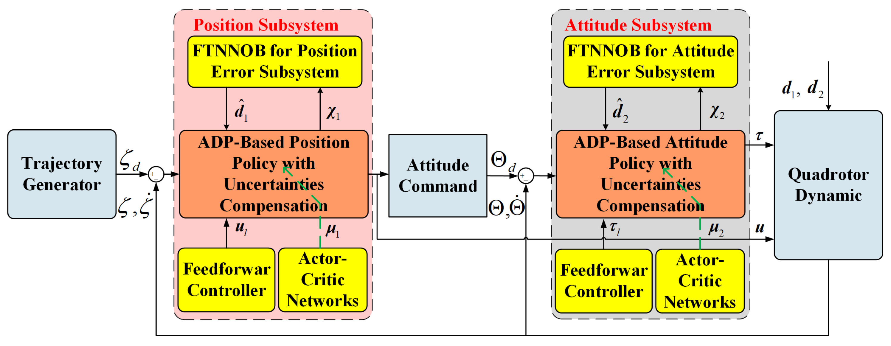
3. Adaptive-Dynamic-Programming-Based Robust Control Design

3.1. Online-Uncertainty-Compensation-Based Fixed-Time NN-Based Observers

Consider the systems (7) with uncertainties; the auxiliary systems are introduced as

$$\begin{array}{c}\hfill {\dot{\widehat{\mathit{e}}}}_i=\mathit{f}\left({\mathit{e}}_i\right)+{\mathit{g}}_i({\mathit{\chi }}_i+{\widehat{\mathit{d}}}_i),\end{array}$$

(9)

where ${\widehat{\mathit{d}}}_i$ are the estimated values of the lumped uncertainties. Define the auxiliary variables as ${\mathbf{\Xi }}_i={\mathit{g}}_i^{†}({\mathit{e}}_i-{\widehat{\mathit{e}}}_i)$ with ${\mathit{g}}_i^{†}$ being pseudo inverse matrices of ${\mathit{g}}_i$. Consider the Assumptions 1 and 2; this yields

$$\begin{array}{c}\hfill ∥{\mathit{d}}_i∥\le h_i{H}_i\left({\mathit{S}}_i\right)={\xi }_i\left({\mathit{S}}_i\right)\end{array}$$

with

$$\begin{array}{c}\hfill \begin{array}{c}{h}_1=\max \left\{u_{\overline{d}},{\alpha }_2,{\alpha }_3,{\alpha }_4\right\},h_2=\max \left\{{\tau }_{\overline{d}},{\alpha }_5,{\alpha }_6,{\alpha }_7\right\},\\ H_1\left({\mathit{S}}_1\right)=1+∥\mathit{\zeta }∥+{∥\dot{\mathit{\zeta }}∥}^2,H_2\left({\mathit{S}}_2\right)=1+∥\mathbf{\Theta }∥+{∥\dot{\mathbf{\Theta }}∥}^2,\end{array}\end{array}$$

where $H_i\left({\mathit{S}}_i\right)$ are defined as the core functions [44]. Furthermore, they are dependent on ${\mathit{S}}_1={[\mathit{\zeta },\dot{\mathit{\zeta }},{\dot{\mathit{\zeta }}}^2]}^{\mathrm{T}}$ and ${\mathit{S}}_2={[\mathbf{\Theta },\dot{\mathbf{\Theta }},{\dot{\mathbf{\Theta }}}^2]}^{\mathrm{T}}$. As pointed out in [45,46], the continuous nonlinear scalar functions ${\xi }_i\left({\mathit{S}}_i\right)$ can be approximated using NNs with Gaussian basis functions:

$$\begin{array}{c}\hfill {\xi }_i\left({\mathit{S}}_i\right)={\mathit{W}}_{fi}^{\mathrm{T}}\mathit{Z}\left({\mathit{S}}_i\right)+{\epsilon }_{fi},\end{array}$$

where $\mathit{Z}\left({\mathit{S}}_i\right)={[Z_1\left({\mathit{S}}_i\right),Z_2\left({\mathit{S}}_i\right),\cdots ,Z_n\left({\mathit{S}}_i\right)]}^{\mathrm{T}}$ are activation function vectors. Furthermore, $Z_n\left({\mathit{S}}_i\right)$ are expressed in detail as

$$\begin{array}{c}\hfill Z_n\left({\mathit{S}}_i\right)=\exp \left(-\frac{{∥{\mathit{S}}_i-{\mathit{\iota }}_{in}∥}^2}{h_{in}^2}\right),\end{array}$$

where ${\mathit{\iota }}_{in}$ and $h_{in}$ are the center vectors and width and n is the sum of the number of the Gaussian basis functions. It is straightforward to show that $\mathit{Z}\left({\mathit{S}}_i\right)$ have norm upper bounds ${ϵ}_i$, that is $∥\mathit{Z}\left({\mathit{S}}_i\right)∥<{ϵ}_i<\infty$ with ${ϵ}_i$ are positive constants. ${\mathit{W}}_{fi}$ denote the optimal weight vectors, and ${\epsilon }_{fi}$ are the approximation errors, in which ${\mathit{W}}_{fi}$ and ${\epsilon }_{fi}$ are bounded, i.e., $∥{\mathit{W}}_{fi}∥\le {\overline{W}}_{fi}$ and $∥{\epsilon }_{fi}∥\le {\overline{\epsilon }}_{fi}$.

In order to reduce the number of parameters for online calculation, the following procedure is designed. Firstly, we have

$$\begin{array}{c}\hfill ∥{\mathit{d}}_i∥\le {\xi }_i\left({\mathit{S}}_i\right)\le ∥{\mathit{W}}_{fi}^{\mathrm{T}}∥∥\mathit{Z}\left({\mathit{S}}_i\right)∥+∥{\epsilon }_{fi}∥\le b_i{Z}_{fi}\end{array}$$

with $b_i=\max \left\{∥{\mathit{W}}_{fi}∥,∥{\epsilon }_{fi}∥\right\},Z_{fi}=1+∥\mathit{Z}\left({\mathit{S}}_i\right)∥$.

Then, the FTNNOBs are established as

$${\widehat{\mathit{d}}}_i=r_{i3}{\mathrm{sig}}^{\frac{m_i}{n_i}}\left({\mathbf{\Xi }}_i\right)+r_{i4}{\mathrm{sig}}^{\frac{p_i}{q_i}}\left({\mathbf{\Xi }}_i\right)+c_i{\widehat{l}}_i{\mathbf{\Xi }}_i{Z}_{fi}^2,$$

(10)

where $m_i,n_i,p_i$ and $q_i$ are positive odd integers satisfying $m_i<n_i,p_i>q_i$. $r_{i3},r_{i4}$, and $c_i$ are positive constants. ${\widehat{l}}_i$ are the estimated values of $l_i=b_i^2$, which are tuned by the following adaptive laws:

$${\dot{\widehat{l}}}_i=-{\varrho }_{i1}{\widehat{l}}_i+c_i{∥{\mathbf{\Xi }}_i∥}^2{Z}_{fi}^2,({\widehat{l}}_i\left(0\right)\ge 0)$$

(11)

with ${\varrho }_{i1}$ being positive constants. The estimation errors of $l_i$ are defined as ${\tilde{l}}_i=l_i-{\widehat{l}}_i$. We have the following result for the proposed procedure.

Lemma 4. 

Based on the proposed adaptive laws (11), there exists positive constants ${\overline{l}}_i$ such that ${\widehat{l}}_i\le {\overline{l}}_i$ and $l_i\le {\overline{l}}_i$.

Proof. 

Select the following positive definite Lyapunov functions:

$$\begin{array}{c}\hfill L_{i1}=\frac{1}{2}{\mathbf{\Xi }}_i^{\mathrm{T}}{\mathbf{\Xi }}_i+\frac{1}{2}{\tilde{l}}_i^2.\end{array}$$

Substituting (10) and (11) into the time derivative of $L_{i1}$ yields

$$\begin{array}{c}\hfill \begin{array}{c}\hfill {\dot{L}}_{i1}\le b_i{Z}_{fi}∥{\mathbf{\Xi }}_i∥-r_{i3}{\left({∥{\mathbf{\Xi }}_i∥}^2\right)}^{\frac{m_i+n_i}{2n_i}}-c_i{\widehat{l}}_i{∥{\mathbf{\Xi }}_i∥}^2{Z}_{fi}^2-c_i{\tilde{l}}_i{∥{\mathbf{\Xi }}_i∥}^2{Z}_{fi}^2+{\varrho }_{i1}{\tilde{l}}_i{\widehat{l}}_i.\end{array}\end{array}$$

(12)

According to Young’s inequality [47], one has

$$\begin{array}{c}\hfill xy\le \frac{{\check{\alpha }}^a}{a}{\left|x\right|}^a+\frac{1}{p{\check{\alpha }}^p}{\left|y\right|}^p,\end{array}$$

where $x,y\in \mathcal{R},\check{\alpha }>0,a>1,p>1$ and $(a-1)(p-1)=1$. Then, one has

$$\begin{array}{c}\hfill \begin{array}{c}\hfill b_i{Z}_{fi}∥{\mathbf{\Xi }}_i∥\le c_i{b}_i^2{∥{\mathbf{\Xi }}_i∥}^2{Z}_{fi}^2+\frac{1}{4c_i}{\varrho }_{i1},{\tilde{l}}_i{\widehat{l}}_i\le -\frac{{\varrho }_{i1}}{2}{\tilde{l}}_i^2+\frac{{\varrho }_{i1}}{2}{l}_i^2.\end{array}\end{array}$$

(13)

According to Lemma 3 and substituting (13) into (12), one can obtain that

$$\begin{array}{c}\hfill \begin{array}{cc}\hfill {\dot{L}}_{i1}\le & -r_{i3}{2}^{\frac{m_i+n_i}{2n_i}}{\left(\frac{1}{2}{∥{\mathbf{\Xi }}_i∥}^2\right)}^{\frac{m_i+n_i}{2n_i}}-{\varrho }_{i1}{2}^{\frac{m_i+n_i}{2n_i}}{\left(\frac{1}{2}{\tilde{l}}_i^2\right)}^{\frac{m_i+n_i}{2n_i}}+{\varrho }_{i1}{\left({\tilde{l}}_i^2\right)}^{\frac{m_i+n_i}{2n_i}}-{\varrho }_{i1}{\tilde{l}}_i^2\hfill \\ \hfill \phantom{=}& +\frac{{\varrho }_{i1}}{2}{l}_i^2+\frac{1}{4c_i}\hfill \\ \hfill \le & -{\pi }_{i1}{L}_{i1}^{a_{i2}}-{\varrho }_{i1}{\tilde{l}}_i^2+{\varrho }_{i1}{\left({\tilde{l}}_i^2\right)}^{a_{i2}}+\frac{{\varrho }_{i1}}{2}{l}_i^2+\frac{1}{4c_i}.\hfill \end{array}\end{array}$$

If ${\tilde{l}}_i^2\ge 1$, one can obtain that

$$\begin{array}{c}\hfill {\varrho }_{i1}{\left({\tilde{l}}_i^2\right)}^{a_{i2}}-{\varrho }_{i1}{\tilde{l}}_i^2\le 0.\end{array}$$

If ${\tilde{l}}_i^2<1$, one can obtain that

$$\begin{array}{c}\hfill 0\le {\varrho }_{i1}{\left({\tilde{l}}_i^2\right)}^{a_{i2}}-{\varrho }_{i1}{\tilde{l}}_i^2\le a_{i1},\end{array}$$

where

$$\begin{array}{c}\hfill \begin{array}{c}\hfill {\pi }_{i1}=\min \left\{r_{i3}{2}^{a_{i2}},{\varrho }_{i1}{2}^{a_{i2}}\right\},a_{i1}={\varrho }_{i1}\left({a_{i2}}^{\frac{a_{i2}}{1-a_{i2}}}-{a_{i2}}^{\frac{1}{1-a_{i2}}}\right)\end{array}\end{array}$$

with $a_{i2}=\frac{m_i+n_i}{2n_i}$. Then, it can further deduced that $L_{i1}\le -{\pi }_{i1}{L}_{i1}^{a_{i2}}+{\vartheta }_{i0}=-L_{i1}^{a_{i2}}({\vartheta }_{i0}-{\pi }_{i1}{L}_{i1}^{-a_{i2}})$ with ${\vartheta }_{i0}=a_{i1}+\frac{{\varrho }_{i1}}{2}{l}_i^2+\frac{1}{4c_i}$. Furthermore, if ${\vartheta }_{i0}-{\pi }_{i1}{L}_{i1}^{-a_{i2}}>0$, $L_{i1}$ will reachan invariant set

$\left\{L_{i1}|L_{i1}\le {\left(\frac{{\pi }_{i1}}{{\vartheta }_{i0}}\right)}^{\frac{1}{a_{i2}}}\right\}$. Thus, one can conclude that $L_{i1}$ and ${\tilde{l}}_i=l_i-{\widehat{l}}_i$ are bounded, and there exists positive constants ${\overline{l}}_i$ such that ${\widehat{l}}_i,l_i\le {\overline{l}}_i$. □

Furthermore, we will show that the proposed FTNNOBs are stable, as shown in the following theorem.

Theorem 1. 

Consider the systems with uncertainties (7); if the FTNNOBs are designed as the form of (10) with ${\widehat{l}}_i$ being updated by (11), the uncertainties’ observation errors ${\tilde{\mathit{d}}}_i={\mathit{d}}_i-{\widehat{\mathit{d}}}_i$ will converge to a bounded region of the origin in a fixed time.

Proof. 

Select a candidate Lyapunov functions in the form of

$$\begin{array}{c}\hfill L_{i2}=\frac{1}{2}{\mathbf{\Xi }}_i^{\mathrm{T}}{\mathbf{\Xi }}_i+\frac{1}{2}{\check{l}}_i^2.\end{array}$$

where ${\check{l}}_i={\overline{l}}_i-{\widehat{l}}_i$. Substituting (10) and (11) into the time derivative of $L_{i2}$, one can achieve

$$\begin{array}{c}\hfill \begin{array}{cc}\hfill {\dot{L}}_{i2}\le & b_i{Z}_{fi}∥{\mathbf{\Xi }}_i∥-r_{i3}{\left({∥{\mathbf{\Xi }}_i∥}^2\right)}^{a_{i2}}-r_{i4}{\left({∥{\mathbf{\Xi }}_i∥}^2\right)}^{a_{i4}}-c_i{\widehat{l}}_i{∥{\mathbf{\Xi }}_i∥}^2{Z}_{fi}^2-c_i{\check{l}}_i{∥{\mathbf{\Xi }}_i∥}^2{Z}_{fi}^2\hfill \\ \hfill \phantom{=}& +{\varrho }_{i1}{\check{l}}_i{\widehat{l}}_i.\hfill \end{array}\end{array}$$

(14)

where $a_{i4}=\frac{p_i+q_i}{2q_i}$. According to Young’s inequality, one has

$$\begin{array}{c}\hfill \begin{array}{c}\hfill b_i{Z}_{fi}∥{\mathbf{\Xi }}_i∥\le c_i{\overline{l}}_i{∥{\mathbf{\Xi }}_i∥}^2{Z}_{fi}^2+\frac{1}{4c_i},{\varrho }_{i1}{\check{l}}_i{\widehat{l}}_i\le -\frac{{\varrho }_{i1}}{2}{\check{l}}_i^2+\frac{{\varrho }_{i1}}{2}{\overline{l}}_i^2.\end{array}\end{array}$$

(15)

Substituting (15) into (14), one can obtain that

$$\begin{array}{c}\hfill \begin{array}{cc}\hfill {\dot{L}}_{i2}\le & -r_{i3}{2}^{a_{i2}}{\left(\frac{1}{2}{∥{\mathbf{\Xi }}_i∥}^2\right)}^{a_{i2}}-{\varrho }_{i1}{2}^{a_{i2}}{\left(\frac{1}{2}{\check{l}}_i^2\right)}^{a_{i2}}-r_{i4}{2}^{a_{i4}}{\left(\frac{1}{2}{∥{\mathbf{\Xi }}_i∥}^2\right)}^{a_{i4}}\hfill \\ \hfill \phantom{=}& -{\varrho }_{i1}{2}^{a_{i4}}{\left(\frac{1}{2}{\check{l}}_i^2\right)}^{a_{i4}}-{\varrho }_{i1}{\check{l}}_i^2+{\varrho }_{i1}{\left({\check{l}}_i^2\right)}^{a_{i2}}+{\varrho }_{i1}{\left({\check{l}}_i^2\right)}^{a_{i4}}+\frac{{\varrho }_{i1}}{2}{\overline{l}}_i^2+\frac{1}{4c_i}.\hfill \end{array}\end{array}$$

If ${\check{l}}_i^2\ge 1$, one can obtain that

$$\begin{array}{c}\hfill {\varrho }_{i1}{\left({\check{l}}_i^2\right)}^{a_{i2}}-{\varrho }_{i1}{\check{l}}_i^2\le 0.\end{array}$$

If ${\check{l}}_i^2<1$, one can obtain that

$$\begin{array}{c}\hfill 0\le {\varrho }_{i1}{\left({\check{l}}_i^2\right)}^{a_{i2}}-{\varrho }_{i1}{\check{l}}_i^2\le a_{i1},\end{array}$$

On account of the inequalities $\left|{\check{l}}_i\right|=\left|{\overline{l}}_i-{\widehat{l}}_i\right|\le \left|{\overline{l}}_i\right|,0<{\widehat{l}}_i<{\overline{l}}_i$ and according to Lemmas 2 and 3, one can further obtain that

$$\begin{array}{c}\hfill {\dot{L}}_{i2}\le -{\pi }_{i1}{L}_{i1}^{a_{i2}}-{\pi }_{i2}{2}^{a_{i3}}{L}_{i1}^{a_{i4}}+{\vartheta }_{i1},\end{array}$$

where ${\pi }_{i1}=\min \left\{r_{i3}{2}^{a_{i2}},{\varrho }_{i1}{2}^{a_{i2}}\right\}$,${\pi }_{i2}=\min \left\{r_{i4}{2}^{a_{i4}},{\varrho }_{i1}{2}^{a_{i4}}\right\},a_{i3}=\frac{q_i-p_i}{2q_i}$, and ${\vartheta }_{i1}=\frac{1}{4c_i}+a_{i1}+{\varrho }_{i1}(\frac{{\overline{l}}_i^2}{2}+{\overline{l}}_i^{2a_{i4}})$. Based on Lemma 1, $L_{i2}$ will reduce to a residual set in fixed time. The settling time can be achieved by $t_{if}\le \frac{1}{{\pi }_{i1}{\omega }_i(1-a_{i2})}+\frac{1}{{\pi }_{i2}{2}^{a_{i3}}{\omega }_i(a_{i4}-1)}$ with $0<{\omega }_i<1$. Defining an augmented vector ${\check{\mathit{X}}}_i={[{\mathbf{\Xi }}_i^{\mathrm{T}},{\check{l}}_i]}^{\mathrm{T}}$, $L_{i2}$ is also represented as $L_{i2}=\frac{1}{2}{\check{\mathit{X}}}_i^{\mathrm{T}}{\check{\mathit{X}}}_i$, and it is bounded by

$$\begin{array}{c}\hfill {\check{\vartheta }}_{i1}=\left\{{\check{\mathit{X}}}_i\mid L_{i2}\left({\check{\mathit{X}}}_i\right)\le \min \left\{{\vartheta }_{i2},{\vartheta }_{i3}\right\}\right\},\end{array}$$

where ${\vartheta }_{i2}={\left(\frac{{\varrho }_{i0}}{{\pi }_{i1}}\right)}^{\frac{1}{a_{i2}}}$ and ${\vartheta }_{i3}={\left(\frac{{\varrho }_{i0}}{{\pi }_{i2}{2}^{a_{i3}}}\right)}^{\frac{1}{a_{i}4}}$ with ${\varrho }_{i0}=\frac{{\vartheta }_{i1}}{1-{\omega }_i}$. Then, one can conclude that

$$\begin{array}{c}\hfill ∥{\mathbf{\Xi }}_i∥\le ∥{\check{\mathit{X}}}_i∥\le \sqrt{2{\overline{\vartheta }}_{i1}}.\end{array}$$

(16)

where ${\overline{\vartheta }}_{i1}=\min \left\{{\vartheta }_{i2},{\vartheta }_{i3}\right\}$. Consider the definition of ${\mathbf{\Xi }}_i$; one has

$$\begin{array}{c}\hfill \begin{array}{cc}\hfill {\dot{\mathbf{\Xi }}}_i=& {\mathit{d}}_i-{\widehat{\mathit{d}}}_i={\mathit{d}}_i-r_{i3}{\mathrm{sig}}^{\frac{m_i}{n_i}}\left({\mathbf{\Xi }}_i\right)-r_{i4}{\mathrm{sig}}^{\frac{p_i}{q_i}}\left({\mathbf{\Xi }}_i\right)-c_i{\widehat{l}}_i{\mathbf{\Xi }}_i{Z}_{fi}^2={\tilde{\mathit{d}}}_i.\hfill \end{array}\end{array}$$

Then, according to the result (16), the upper norm bounds of ${\tilde{\mathit{d}}}_i$ are given by

$$\begin{array}{c}\hfill \begin{array}{cc}\hfill ∥{\tilde{\mathit{d}}}_i∥\le & ∥{\mathit{d}}_i∥+r_{i3}∥{\mathrm{sig}}^{\frac{m_i}{n_i}}\left({\mathbf{\Xi }}_i\right)∥+r_{i4}∥{\mathrm{sig}}^{\frac{p_i}{q_i}}\left({\mathbf{\Xi }}_i\right)∥+c_i{\overline{l}}_i{Z}_{fi}^2∥{\mathbf{\Xi }}_i∥\hfill \\ \hfill \le & b_i(1+{ϵ}_i)+3r_{i3}{\left(\sqrt{2{\overline{\vartheta }}_{i1}}\right)}^{\frac{m_i}{n_i}}+3r_{i4}{\left(\sqrt{2{\overline{\vartheta }}_{i1}}\right)}^{\frac{p_i}{q_i}}+c_i{\overline{l}}_i\sqrt{2{\overline{\vartheta }}_{i1}}{(1+{ϵ}_i)}^2.\hfill \end{array}\end{array}$$

Based on the above analysis and the selection pf appropriate parameter values, the uncertainties’ observation errors ${\tilde{\mathit{d}}}_i$ will converge to a bounded region of origin in a fixed time. □

Remark 1. 

Compared with previous NN-based observer methods, it is obvious that the proposed FTNNOBs only need to estimate a scalar parameter online instead of a weight vector or matrix, which reduces the computational complexities. Moreover, the fixed-time convergence of the estimation error is guaranteed.

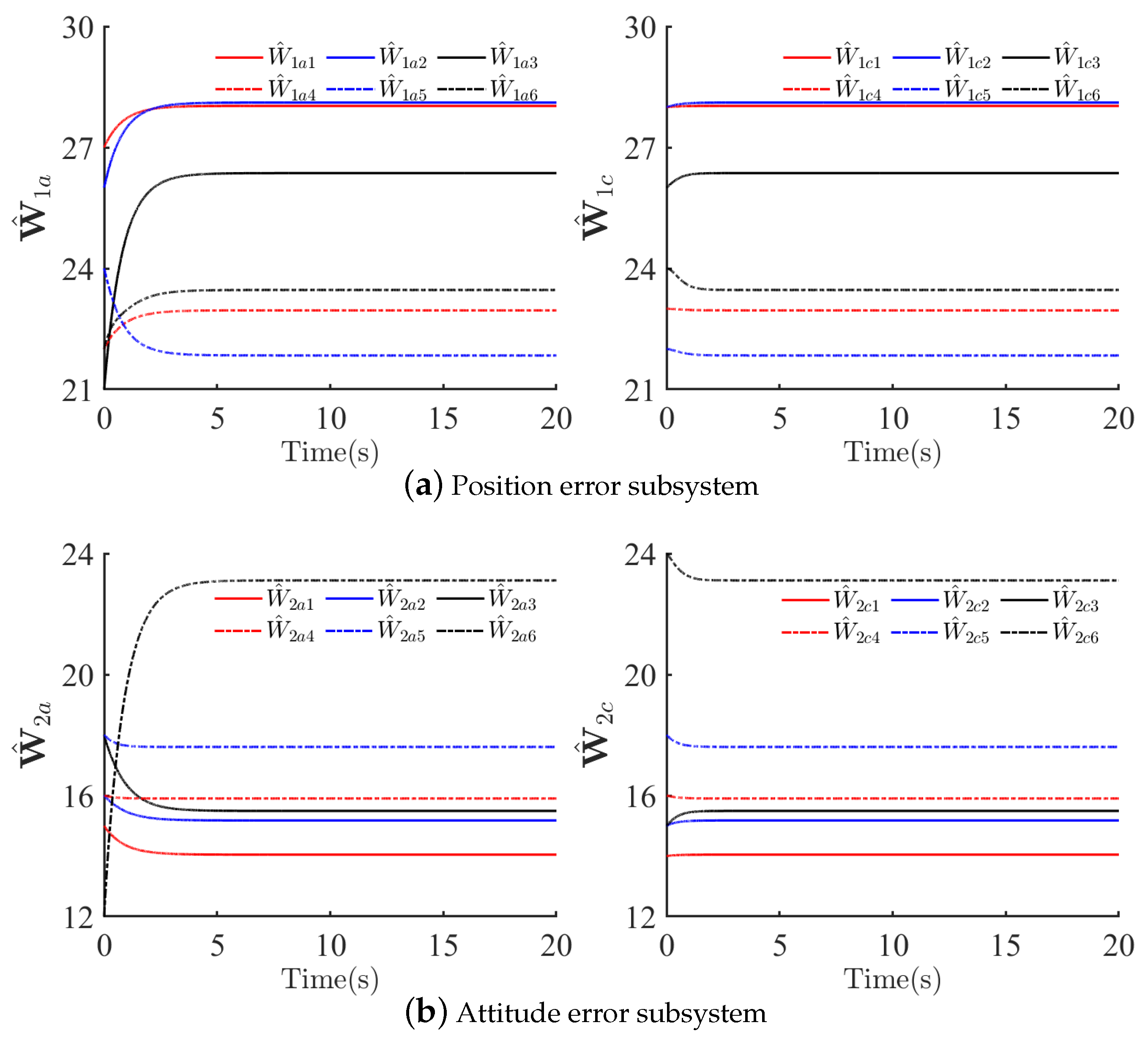
3.2. ADP-Based Nominal Optimal Control Design

Consider the nominal systems of (7):

$$\begin{array}{c}\hfill {\dot{\mathit{e}}}_i=\mathit{f}\left({\mathit{e}}_i\right)+{\mathit{g}}_i{\mathit{\mu }}_i.\end{array}$$

where ${\mathit{\mu }}_i$ is the approximated optimal control policies to be designed. According to [17,26,33], the infinite horizon cost functions can be defined as

$$\begin{array}{c}\hfill V_i\left({\mathit{e}}_i\left(0\right)\right)={\int }_0^{\infty }\left({\mathit{e}}_i^{\mathrm{T}}{\mathit{Q}}_i{\mathit{e}}_i+{\mathit{\mu }}_i^{\mathrm{T}}{\mathit{R}}_i{\mathit{\mu }}_i\right)dt,\end{array}$$

(17)

where ${\mathit{Q}}_i$ and ${\mathit{R}}_i$ are assumed to be positive definite diagonal constant matrices. Assuming that the optimal policies ${\mathit{\mu }}_i^{*}$ exist, the corresponding optimally cost functions of (17) are formulated as

$$\begin{array}{c}\hfill \begin{array}{c}\hfill V_i^{*}\left({\mathit{e}}_i\left(0\right)\right)=\underset{{\mathit{\mu }}_i\in {\mathbf{\Psi }}_i\left({\mathit{\varpi }}_i\right)}{\min }\left({\int }_0^{\infty }\left({\mathit{e}}_i^{\mathrm{T}}{\mathit{Q}}_i{\mathit{e}}_i+{\mathit{\mu }}_i^{\mathrm{T}}{\mathit{R}}_i{\mathit{\mu }}_i\right)dt\right),\end{array}\end{array}$$

(18)

where ${\mathbf{\Psi }}_i\left({\mathit{\varpi }}_i\right)$ are the admissible sets on the compact sets ${\mathit{\varpi }}_i$. Taking the time derivative of (18), one can obtain the Hamilton–Jacobi–Bellman (HJB) equations:

$$\begin{array}{c}\hfill \begin{array}{cc}& H_i\left({\mathit{e}}_i,{\mathit{\mu }}_i^{*},\nabla V_i^{*}\left({\mathit{e}}_i\right)\right)={\nabla }^{\mathrm{T}}{V}_i^{*}\left(\mathit{f}\left({\mathit{e}}_i\right)+{\mathit{g}}_i{\mathit{\mu }}_i^{*}\right)+{{\mathit{\mu }}_i^{*}}^{\mathrm{T}}{\mathit{R}}_i{\mathit{\mu }}_i^{*}+{\mathit{e}}_i^{\mathrm{T}}{\mathit{Q}}_i{\mathit{e}}_i=0,\hfill \end{array}\end{array}$$

(19)

where $\nabla =\partial /\partial {\mathit{e}}_i$ are the Jacobian matrices. Then, the optimal control policies ${\mathit{\mu }}_i^{*}$ can be derived by taking the partial derivative for (19) with respect to ${\mathit{\mu }}_i^{*}$:

$$\begin{array}{c}\hfill {\mathit{\mu }}_i^{*}=-\frac{1}{2}{\mathit{R}}_i^{-1}{\mathit{g}}_i^{\mathrm{T}}\nabla V_i^{*}\left({\mathit{e}}_i\right).\end{array}$$

(20)

Substituting (20) into (19), the HJB equations can be further written as

$$\begin{array}{c}\hfill \begin{array}{c}\hfill 0=\nabla V_i^{*\mathrm{T}}\left({\mathit{e}}_i\right)f\left({\mathit{e}}_i\right)+{\mathit{e}}_i^{\mathrm{T}}{\mathit{Q}}_i{\mathit{e}}_i-\frac{1}{4}\nabla V^{*\mathrm{T}}\left({\mathit{e}}_i\right){\mathit{g}}_i{\mathit{R}}_i^{-1}{\mathit{g}}_i^{\mathrm{T}}\nabla V_i^{*}\left({\mathit{e}}_i\right).\end{array}\end{array}$$

(21)

However, for the HJB Equation (21), it is difficult to obtain the analytical solutions owing to their nonlinearity. Therefore, the AC NN technique will be introduced to solve this problem.

For all ${\mathit{e}}_i\in {\mathit{\varpi }}_i$, the optimal cost functions ${V_i}^{*}\left({\mathit{e}}_i\right)$ can be approximated by

$$\begin{array}{c}\hfill {V_i}^{*}\left({\mathit{e}}_i\right)={\mathit{W}}_i^{\mathrm{T}}{\mathit{\sigma }}_i\left({\mathit{e}}_i\right)+{\epsilon }_i,\end{array}$$

where ${\mathit{W}}_i\in {\mathcal{R}}^n$ denote the unknown ideal weight vectors, and ${\mathit{\sigma }}_i\left({\mathit{e}}_i\right)\in {\mathcal{R}}^n$ are the basis function vectors with n being the number of hidden layer neurons; ${\epsilon }_i$ is the approximation error. In addition, the optimal control policies ${\mathit{\mu }}_i^{*}$ can be reconstructed in the form of

$$\begin{array}{c}\hfill {\mathit{\mu }}_i^{*}=-\frac{1}{2}{\mathit{R}}_i^{-1}{\mathit{g}}_i^T({\nabla }^{\mathrm{T}}{\mathit{\sigma }}_i\left({\mathit{e}}_i\right){\mathit{W}}_i+\nabla {\epsilon }_i).\end{array}$$

Two NNs (i.e., AC NNs) are usually utilized to approximate the control policies and optimal cost functions, respectively. The approximation results can be given by

$$V_i\left({\mathit{e}}_i\right)={\widehat{\mathit{W}}}_{ic}^{\mathrm{T}}{\mathit{\sigma }}_i\left({\mathit{e}}_i\right),$$

(22)

$${\mathit{\mu }}_i=-\frac{1}{2}{\mathit{R}}_i^{-1}{\mathit{g}}_i^{\mathrm{T}}{\nabla }^{\mathrm{T}}{\mathit{\sigma }}_i\left({\mathit{e}}_i\right){\widehat{\mathit{W}}}_{ia},$$

(23)

where ${\widehat{\mathit{W}}}_{ia},{\widehat{\mathit{W}}}_{ic}\in {\mathcal{R}}^n$ denote the weight vectors of the AC NNs.

Substituting (22) and (23) into (21), one can obtain the approximate results of the HJB equations:

$$\begin{array}{c}\hfill \begin{array}{c}\hfill {\widehat{H}}_i={\widehat{\mathit{W}}}_{ic}^{\mathrm{T}}\nabla {\mathit{\sigma }}_i(\mathit{f}\left({\mathit{e}}_i\right)+{\mathit{e}}_i^{\mathrm{T}}{\mathit{Q}}_i{\mathit{e}}_i-\frac{1}{2}{\mathit{g}}_i{\mathit{R}}_i^{-1}{{\mathit{g}}^{\mathrm{T}}}_i{\nabla }^{\mathrm{T}}{\mathit{\sigma }}_i\left({\mathit{e}}_i\right){\widehat{\mathit{W}}}_{ia})+\frac{1}{4}{\widehat{\mathit{W}}}_{ia}^{\mathrm{T}}{\mathit{B}}_i{\widehat{\mathit{W}}}_{ia}=E_i,\end{array}\end{array}$$

where ${\widehat{H}}_i=H_i\left({\mathit{e}}_i,{\mathit{\mu }}_i,\nabla {\mathit{\sigma }}_i\left({\mathit{e}}_i\right)\right)$ and ${\mathit{B}}_i=\nabla {\mathit{\sigma }}_i\left({\mathit{e}}_i\right){\mathit{g}}_i{\mathit{R}}_i^{-1}{{\mathit{g}}^{\mathrm{T}}}_i{\nabla }^{\mathrm{T}}{\mathit{\sigma }}_i\left({\mathit{e}}_i\right)$. $E_i$ represent the Bellman residual errors. Two positive functions are constructed as

$$\begin{array}{c}\hfill {\kappa }_i\left(t\right)={({\widehat{\mathit{W}}}_{ia}-{\widehat{\mathit{W}}}_{ic})}^{\mathrm{T}}({\widehat{\mathit{W}}}_{ia}-{\widehat{\mathit{W}}}_{ic}).\end{array}$$

Then, calculating the time derivative of ${\kappa }_i\left(t\right)$ along ${\widehat{\mathit{W}}}_{ia}$ and ${\widehat{\mathit{W}}}_{ic}$, one has

$$\begin{array}{c}\hfill \frac{d{\kappa }_i\left(t\right)}{dt}=\frac{\partial {\kappa }_i\left(t\right)}{\partial {\widehat{\mathit{W}}}_{ia}}{\dot{\widehat{\mathit{W}}}}_{ia}+\frac{\partial {\kappa }_i\left(t\right)}{\partial {\widehat{\mathit{W}}}_{ic}}{\dot{\widehat{\mathit{W}}}}_{ic}.\end{array}$$

(24)

The weight update laws of ${\widehat{\mathit{W}}}_{ia},{\widehat{\mathit{W}}}_{ic}$ are proposed in the form of

$${\dot{\widehat{\mathit{W}}}}_{ic}=-k_{i1}{\Lambda }_i{\widehat{\mathit{W}}}_{ic}+k_{i3}{\mathit{\beta }}_{i1},$$

(25)

$${\dot{\widehat{\mathit{W}}}}_{ia}=-k_{i1}{\Lambda }_i{\widehat{\mathit{W}}}_{ic}-k_{i2}\left({\widehat{\mathit{W}}}_{ia}-{\widehat{\mathit{W}}}_{ic}\right)+k_{i3}{\mathit{\beta }}_{i1},$$

(26)

where $k_{i1},k_{i2}$, and $k_{i3}$ are the learning rates. $k_{i1}$ and $k_{i2}$ are positive constants, and $k_{i3}=∥{\mathit{Q}}_i∥$. ${\mathit{\beta }}_{i1}=\frac{{\mathit{\beta }}_{i2}}{1+{\mathit{\beta }}_{i2}^{\mathrm{T}}{\mathit{\beta }}_{i2}}$ with ${\mathit{\beta }}_{i2}={\nabla }^{\mathrm{T}}{\mathit{\sigma }}_i\left({\mathit{e}}_i\right)·{\mathit{e}}_i$. ${\Lambda }_i=r_{i1}∥{\mathit{\beta }}_{i1}∥+r_{i2}$ with $r_{i1}$ and $r_{i2}$ being positive constants. In addition, the AC NNs’ weight errors are defined as ${\tilde{\mathit{W}}}_{ia}={\mathit{W}}_i-{\widehat{\mathit{W}}}_{ia}$ and ${\tilde{\mathit{W}}}_{ic}={\mathit{W}}_i-{\widehat{\mathit{W}}}_{ic}$. Substituting (25) and (26) into (24) yields

$$\begin{array}{c}\hfill \frac{d{\kappa }_i\left(t\right)}{dt}=-2k_{i2}{({\widehat{\mathit{W}}}_{ia}-{\widehat{\mathit{W}}}_{ic})}^{\mathrm{T}}({\widehat{\mathit{W}}}_{ia}-{\widehat{\mathit{W}}}_{ic})\le 0.\end{array}$$

(27)

According to (27), it can be further concluded that ${\kappa }_i\left(t\right)=0$ will be finally achieved under the weight update laws (25) and (26). According to [48], the approximate optimal solutions ${\mathit{\mu }}_i$ are expected to satisfy the Bellman residual errors $E_i\to 0$. Furthermore, if $E_i=0$ has a unique solution, it is equivalent to the following equations:

$$\begin{array}{c}\hfill \begin{array}{cc}\hfill \frac{\partial E_i}{\partial {\widehat{\mathit{W}}}_{ia}}& =\frac{1}{2}{\mathit{B}}_i({\widehat{\mathit{W}}}_{ia}-{\widehat{\mathit{W}}}_{ic})={\mathit{0}}_{n\times 1}.\hfill \end{array}\end{array}$$

(28)

Obviously, based on the results ${\kappa }_i\left(t\right)=0$, the derivation of (27) and (28) will be satisfied.

3.3. Adaptive-Dynamic-Programming-Based Robust Control Law Design

Based on the reconstructed information of the above-proposed FTNNOBs ${\widehat{\mathit{d}}}_i$ in (10) and the designed approximate optimal control policies ${\mathit{\mu }}_i$ in (23), the feedforward method was employed to compensate the approximate optimal control policies to restrain the lumped uncertainties. Then, the ADP-based robust control laws can be designed as

$$\begin{array}{c}\hfill {\mathit{\chi }}_i={\mathit{\mu }}_i-{\widehat{\mathit{d}}}_i.\end{array}$$

(29)

Assumption 3. 

For all ${\mathit{e}}_i\in {\mathit{\varpi }}_i$, the following conditions $∥\nabla {\mathit{\sigma }}_i\left({\mathit{e}}_i\right)∥\le \nabla {\overline{\sigma }}_i,∥{\mathit{W}}_i∥\le {\overline{W}}_i$, and $∥\nabla {\epsilon }_i∥\le \nabla {\overline{\epsilon }}_i$ are satisfied with $\nabla {\overline{\sigma }}_i,{\overline{W}}_i$ and $\nabla {\overline{\epsilon }}_i$ being positive constants.

With the designed control law, we can show that the closed-loop system is stable in the following theorem.

Theorem 2. 

Consider the systems in (7), Assumptions 1 and 3, and the cost function (18); if the proposed ADP-based robust control laws are defined as the form of (29) with the FTNNOBs (10) and the approximate optimal laws (23), then the tracking errors ${\mathit{e}}_i$ and AC NNs’ weight errors ${\tilde{\mathit{W}}}_{ia},{\tilde{\mathit{W}}}_{ic}$ can be guaranteed to be ultimately uniformly bounded (UUB).

Proof. 

Select a candidate Lyapunov functions as

$$\begin{array}{c}\hfill L_{i3}=V^{*}\left({\mathit{e}}_i\right)+\frac{{\rho }_{i1}}{2}{\tilde{\mathit{W}}}_{ia}^{\mathrm{T}}{\tilde{\mathit{W}}}_{ia}+\frac{{\rho }_{i2}}{2}{\tilde{\mathit{W}}}_{ic}^{\mathrm{T}}{\tilde{\mathit{W}}}_{ic},\end{array}$$

where ${\rho }_{i1}$ and ${\rho }_{i2}$ are positive constants with ${\rho }_{i1}>{\rho }_{i2}$. Calculating the time derivative of $L_{i3}$ yields

$$\begin{array}{cc}\hfill {\dot{L}}_{i3}=& {\nabla }^{\mathrm{T}}{V}^{*}(\mathit{f}\left({\mathit{e}}_i\right)+{\mathit{g}}_i{\mathit{\mu }}_i^{*})+{\nabla }^{\mathrm{T}}{V}^{*}({\mathit{g}}_i{\mathit{\mu }}_i-{\mathit{g}}_i{\mathit{\mu }}_i^{*})+{\nabla }^{\mathrm{T}}{V}^{*}{\mathit{g}}_i({\mathit{d}}_i-{\widehat{\mathit{d}}}_i)\hfill \\ & -{\rho }_{i2}\tilde{\mathit{W}}{}_{ic}^{\mathrm{T}}{\dot{\widehat{\mathit{W}}}}_{ic}-{\rho }_{i1}\tilde{\mathit{W}}{}_{ia}^{\mathrm{T}}{\dot{\widehat{\mathit{W}}}}_{ia}\hfill \\ \hfill =& -{\mathit{e}}_i^{\mathrm{T}}\mathit{Q}{\mathit{e}}_i-\frac{1}{4}{\mathit{W}}_i^T{\mathit{B}}_i{\mathit{W}}_i+\frac{k_{i1}{\rho }_{i1}}{2}{\mathit{W}}_i^{\mathrm{T}}{\Lambda }_i{\mathit{W}}_i-\frac{1}{2}{\mathit{W}}_i^T\nabla {\mathit{\sigma }}_i\left({\mathit{e}}_i\right){\mathit{g}}_i{\mathit{R}}_i^{-1}{\mathit{g}}_i^{\mathrm{T}}\nabla {\epsilon }_i\hfill \\ \hfill \phantom{=}& -\frac{1}{2}{\nabla }^{\mathrm{T}}{\epsilon }_i{\mathit{g}}_i{\mathit{R}}_i^{-1}{\mathit{g}}_i^{\mathrm{T}}{\nabla }^{\mathrm{T}}{\mathit{\sigma }}_i\left({\mathit{e}}_i\right){\tilde{\mathit{W}}}_{ia}+\frac{1}{2}{\mathit{W}}_i^T\nabla {\mathit{\sigma }}_i\left({\mathit{e}}_i\right){\mathit{g}}_i{\mathit{R}}_i^{-1}{\mathit{g}}_i^{\mathrm{T}}\nabla {\epsilon }_i\hfill \\ \hfill \phantom{=}& -\frac{k_{i1}{\rho }_{i1}}{2}\tilde{\mathit{W}}{}_{ic}^{\mathrm{T}}{\Lambda }_i{\tilde{\mathit{W}}}_{ic}-\frac{k_{i1}{\rho }_{i1}}{2}\widehat{\mathit{W}}{}_{ic}^{\mathrm{T}}{\Lambda }_i{\widehat{\mathit{W}}}_{ic}+\frac{1}{4}{\nabla }^{\mathrm{T}}{\epsilon }_i{\mathit{g}}_i{\mathit{R}}_i^{-1}{\mathit{g}}_i^{\mathrm{T}}\nabla {\epsilon }_i+k_{i1}{\rho }_{i2}\tilde{\mathit{W}}{}_{ia}^{\mathrm{T}}{\Lambda }_i{\widehat{\mathit{W}}}_{ic}\hfill \\ \hfill \phantom{=}& -k_{i3}{\rho }_{i2}\tilde{\mathit{W}}{}_{ic}^{\mathrm{T}}{\mathit{\beta }}_{i1}-k_{i3}{\rho }_{i1}\tilde{\mathit{W}}{}_{ia}^{\mathrm{T}}{\mathit{\beta }}_{i1}-k_{i2}{\rho }_{i2}\tilde{\mathit{W}}{}_{ia}^{\mathrm{T}}{\tilde{\mathit{W}}}_{ia}+k_{i2}{\rho }_{i2}\tilde{\mathit{W}}{}_{ia}^{\mathrm{T}}{\tilde{\mathit{W}}}_{ic}+{\mathit{\vartheta }}_{i4}\hfill \end{array}$$

where ${\mathit{\vartheta }}_{i4}=({\nabla }^{\mathrm{T}}{\mathit{\sigma }}_i\left({\mathit{e}}_i\right){\mathit{W}}_i+{\nabla }^{\mathrm{T}}{\epsilon }_i){\mathit{g}}_i{\tilde{\mathit{d}}}_i$. Based on Assumptions 2 and 3, it is reasonable to assume that $\frac{1}{2}\nabla {\mathit{\sigma }}_i\left({\mathit{e}}_i\right){\mathit{g}}_i{\mathit{R}}_i^{-1}{{\mathit{g}}^{\mathrm{T}}}_i{\nabla }^{\mathrm{T}}{\mathit{\sigma }}_i\left({\mathit{e}}_i\right)$, $\frac{1}{2}{\nabla }^{\mathrm{T}}{\epsilon }_i{\mathit{g}}_i{\mathit{R}}_i^{-1}{\mathit{g}}_i^{\mathrm{T}}\nabla {\epsilon }_i$, and $({\nabla }^{\mathrm{T}}{\mathit{\sigma }}_i\left({\mathit{e}}_i\right){\mathit{W}}_i+{\nabla }^{\mathrm{T}}{\epsilon }_i){\mathit{g}}_i$ are norm-bounded. From Theorem 1, since the disturbance error bounds are fixed-time stable, we can assume that ${\tilde{\mathit{d}}}_i$ are also norm-bounded, that is $∥{\tilde{\mathit{d}}}_i∥\le d_{iM}$ with $d_{iM}$ being positive constants. Then, one has

$$\begin{array}{cc}& \begin{array}{c}∥\frac{1}{2}\nabla {\mathit{\sigma }}_i\left({\mathit{e}}_i\right){\mathit{g}}_i{\mathit{R}}_i^{-1}{{\mathit{g}}^{\mathrm{T}}}_i{\nabla }^{\mathrm{T}}{\mathit{\sigma }}_i\left({\mathit{e}}_i\right)∥\le b_{{\mathit{D}}_i},∥\frac{1}{2}{\nabla }^{\mathrm{T}}{\epsilon }_i{\mathit{g}}_i{\mathit{R}}_i^{-1}{\mathit{g}}_i^{\mathrm{T}}\nabla {\epsilon }_i+{\mathit{\vartheta }}_{i4}∥\le {\alpha }_{i8}\end{array}\hfill \end{array}$$

where $b_{{\mathit{D}}_i}$ are positive constants. Consider the inequality $∥{\mathit{\beta }}_1∥\le \nabla {\overline{\sigma }}_i∥{\mathit{e}}_i∥$; the following inequalities can be obtained by using Young’s inequality:

$$-k_{i3}{\rho }_{i2}\tilde{\mathit{W}}{}_{ic}^{\mathrm{T}}{\mathit{\beta }}_{i1}\le \frac{\nabla {\overline{\sigma }}_i^2}{2}{∥{\tilde{\mathit{W}}}_{ic}∥}^2+\frac{k_{i3}^2{\rho }_{i2}^2}{2}{∥{\mathit{e}}_i∥}^2,$$

(30)

$$-k_{i3}{\rho }_{i1}\tilde{\mathit{W}}{}_{ia}^{\mathrm{T}}{\mathit{\beta }}_{i1}\le \frac{\nabla {\overline{\sigma }}_i^2}{2}{∥{\tilde{\mathit{W}}}_{ia}∥}^2+\frac{k_{i3}^2{\rho }_{i1}^2}{2}{∥{\mathit{e}}_i∥}^2.$$

(31)

In addition, there exist constants $b_{iQ}$ satisfying $b_{iQ}<{\lambda }_{\min }\left({\mathit{Q}}_i\right)$. By utilizing the above inequalities (30) and (31), one can further obtain that

$$\begin{array}{c}\hfill \begin{array}{cc}\hfill {\dot{L}}_{i3}\le & -(b_{iQ}-\frac{k_{i3}^2{\rho }_{i1}^2}{2}-\frac{k_{i3}^2{\rho }_{i2}^2}{2}){∥{\mathit{e}}_i∥}^2-\frac{k_{i2}{\rho }_{i2}-k_{i1}{\rho }_{i2}{\gamma }_i-b_{{\mathit{D}}_i}-{\nabla {\overline{\sigma }}_i}^2}{2}{∥{\tilde{\mathit{W}}}_{ia}∥}^2+{\alpha }_{i8}\hfill \\ \hfill \phantom{=}& -\frac{k_{i1}{\rho }_{i1}{r}_{i2}-k_{i2}{\rho }_{i2}-{\nabla {\overline{\sigma }}_i}^2}{2}{∥{\tilde{\mathit{W}}}_{ic}∥}^2+{\alpha }_{i9},\hfill \end{array}\end{array}$$

(32)

where ${\gamma }_i={\Lambda }_{\max }=r_{i1}{∥{\mathit{\beta }}_{i1}∥}_{\max }+r_{i2}$ and ${\alpha }_{i9}=\frac{k_{i1}{\rho }_{i1}{\gamma }_i}{2}{\overline{W}}_i^2$. Then, we can select the parameters $k_{i1},k_{i2}$, $k_{i3}$, such that $2b_{iQ}-k_{i3}^2{\rho }_{i1}^2-k_{i3}^2{\rho }_{i2}^2>0$, $k_{i2}{\rho }_{i2}-k_{i1}{\rho }_{i2}{\gamma }_i-b_{{\mathit{D}}_i}-{\nabla {\overline{\sigma }}_i}^2>0$, and $k_{i1}{\rho }_{i1}{r}_{i2}-k_{i2}{\rho }_{i2}-{\nabla {\overline{\sigma }}_i}^2>0$ hold. Furthermore, one can conclude that ${\dot{L}}_{i3}\le 0$ when the condition:

$$\begin{array}{c}\hfill \left\{\begin{array}{c}∥{\mathit{e}}_i∥>\sqrt{\frac{2{\alpha }_{i8}}{2b_{iQ}-k_{i3}^2{\rho }_{i1}^2-k_{i3}^2{\rho }_{i2}^2}}\\ ∥{\tilde{\mathit{W}}}_{ia}∥>\sqrt{\frac{2{\alpha }_{i9}}{k_{i2}{\rho }_{i2}-k_{i1}{\rho }_{i2}{\gamma }_i-b_{{\mathit{D}}_i}-{\nabla {\overline{\sigma }}_i}^2}}\mathrm{or}∥{\tilde{\mathit{W}}}_{ic}∥>\sqrt{\frac{2{\alpha }_{i9}}{k_{i1}{\rho }_{i1}{r}_{i2}-k_{i2}{\rho }_{i2}-{\nabla {\overline{\sigma }}_i}^2}}\hfill \end{array}\right.\end{array}$$

is satisfied. Therefore, (32) indicates that the error states of the systems (7) and the AC NNs’ weight errors are UUB stable. □

Remark 2. 

Different from [16,25], we designed weight update laws of the AC NNs that avoid the use of the PE condition by using an adaptive method, where ${\Lambda }_i$ are designed to guarantee stable convergence performances of ${\tilde{\mathit{W}}}_{ic}$ and ${\tilde{\mathit{W}}}_{ia}$. Moreover, the positive constants $r_{i2}$ are introduced in ${\Lambda }_i$ to guarantee ${\tilde{\mathit{W}}}_{ic}$ and ${\tilde{\mathit{W}}}_{ia}$ can converge to a neighborhood of the origin when $∥{\mathit{\beta }}_{i1}∥=0$.

Remark 3. 

In [48,49], the critic NNs’ weight update law only contains a term similar to the first term of (31), which makes the convergence performances of the weights depend heavily on the initial weights. For instance, it is obvious that the training process of the AC NNs’ weights can be broken when the initial weights are set to zero. To emphasize the role of the system states, the second term in the critic NNs’ weight update laws (31) is added to improve the efficiency of the data utilization and the adaption capability of AC NNs.

4. Simulation

Numerical simulations are presented to verify the effectiveness and fine performances of the proposed ADP-based robust trajectory-tracking-control scheme (denoted as ADPFTNs) in this section. Firstly, the robust performances of the proposed ADPFTNs in (29) were verified in the case of external disturbances and parameter uncertainties. Then, we demonstrate the superior ability of the proposed ADPFTNs in balancing control performances and cost. The initial position vector was selected as $\mathit{\zeta }\left(0\right)={[0.1,-0.2,0.131]}^{\mathrm{T}}\mathrm{m}$. The desired position trajectory was ${\mathit{\zeta }}_d={[0.5\sin \left(0.6t\right),0.5\cos \left(0.6t\right),0.5+\frac{3t}{50}]}^{\mathrm{T}}\mathrm{m}$. The desired yaw angle was ${\mathit{\psi }}_d=0\mathrm{rad}$. The basis function vectors are

$$\begin{array}{c}\hfill \begin{array}{c}\hfill {\mathit{\sigma }}_1\left({\mathit{e}}_1\right)={[0.5x_e^2,0.5y_e^2,0.5z_e^2,x_e{\dot{x}}_e,y_e{\dot{y}}_e,z_e{\dot{z}}_e]}^{\mathrm{T}},{\mathit{\sigma }}_2\left({\mathit{e}}_2\right)={[0.5{\varphi }_e^2,0.5{\theta }_e^2,0.5{\psi }_e^2,{\varphi }_e{\dot{\varphi }}_e,{\theta }_e{\dot{\theta }}_e,{\psi }_e{\dot{\psi }}_e]}^{\mathrm{T}}.\end{array}\end{array}$$

The initial weight vectors are

$$\begin{array}{c}\hfill \begin{array}{cc}\hfill {\mathit{W}}_{1a}\left(0\right)& ={[27,26,21,22,24,22]}^{\mathrm{T}},{\mathit{W}}_{2a}\left(0\right)={[15,16,18,16,18,12]}^{\mathrm{T}},\hfill \\ \hfill {\mathit{W}}_{1c}\left(0\right)& ={[28,28,26,23,22,24]}^{\mathrm{T}},{\mathit{W}}_{2c}\left(0\right)={[14,15,15,16,18,24]}^{\mathrm{T}}.\hfill \end{array}\end{array}$$

In addition, the main parameters of the quadrotor UAV are given as $m_0=1.2\mathrm{kg}$, $g=9.81\mathrm{m}/{\mathrm{s}}^2$, ${\mathit{J}}_0=\mathrm{diag}\left\{0.125,0.125,0.25\right\}\mathrm{kg}·{\mathrm{m}}^2$, $J_r=0.002\mathrm{kg}·{\mathrm{m}}^2$, and $k_{10},k_{20},\cdots ,k_{60}=0.01$.

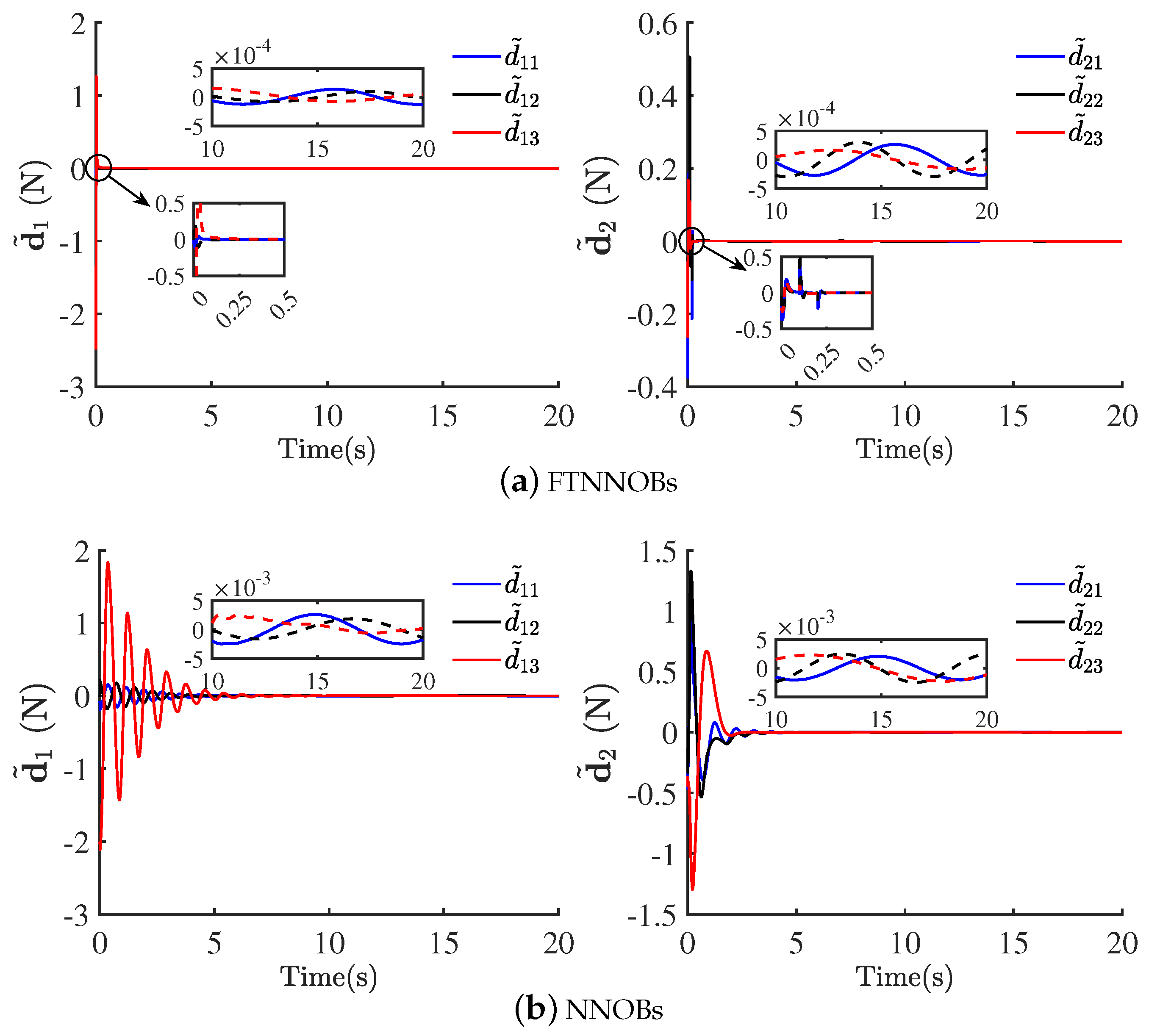
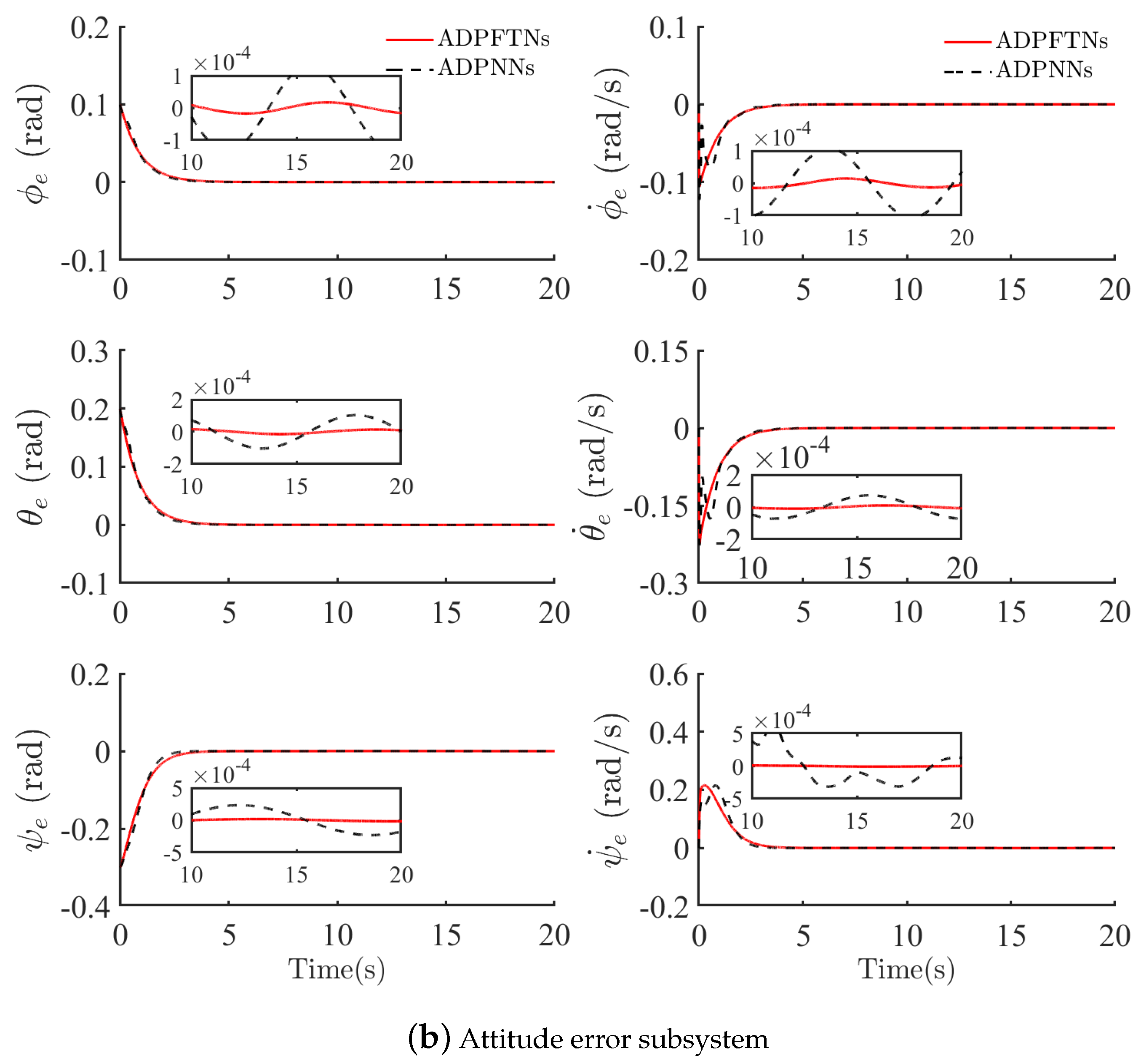
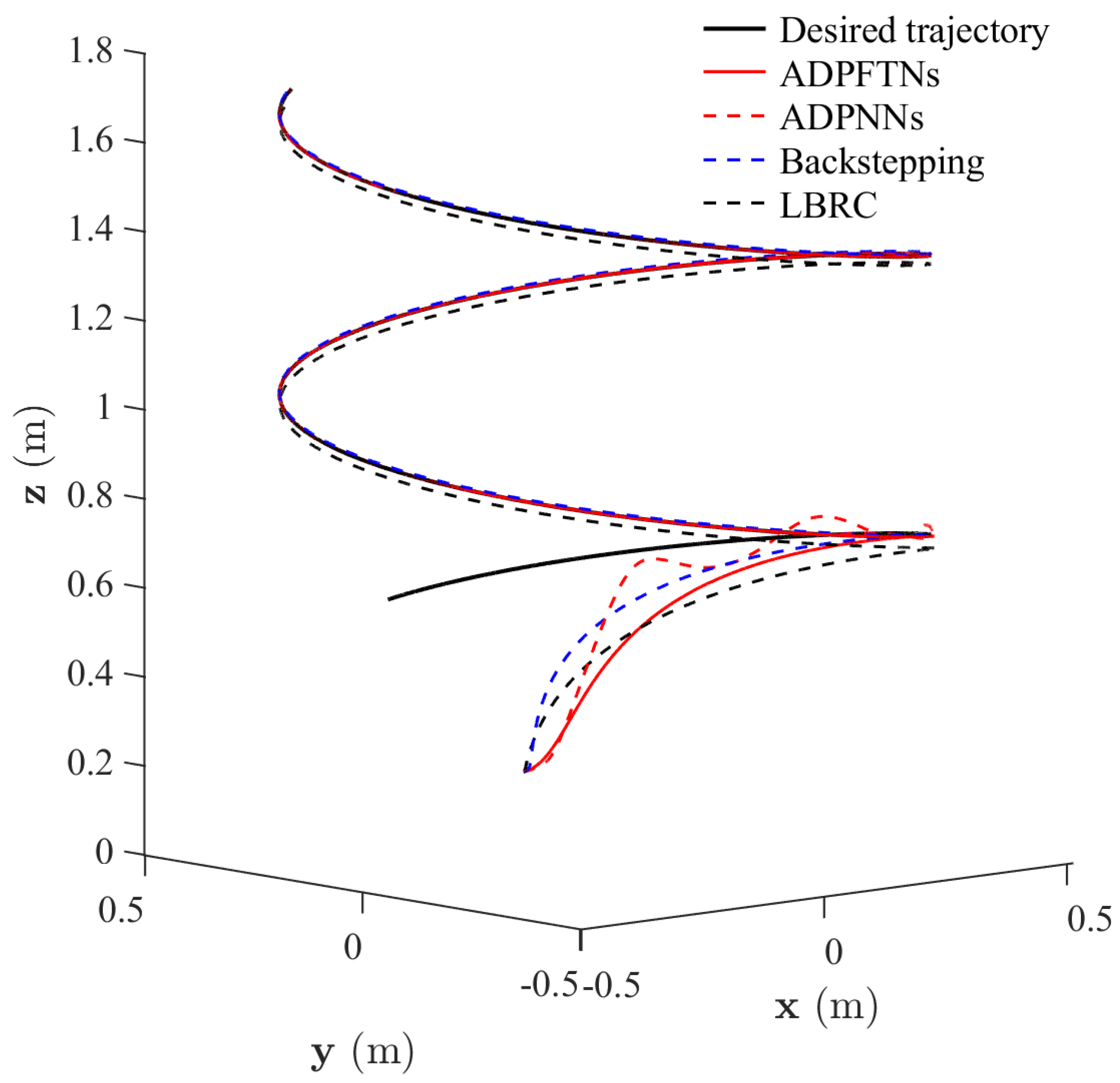
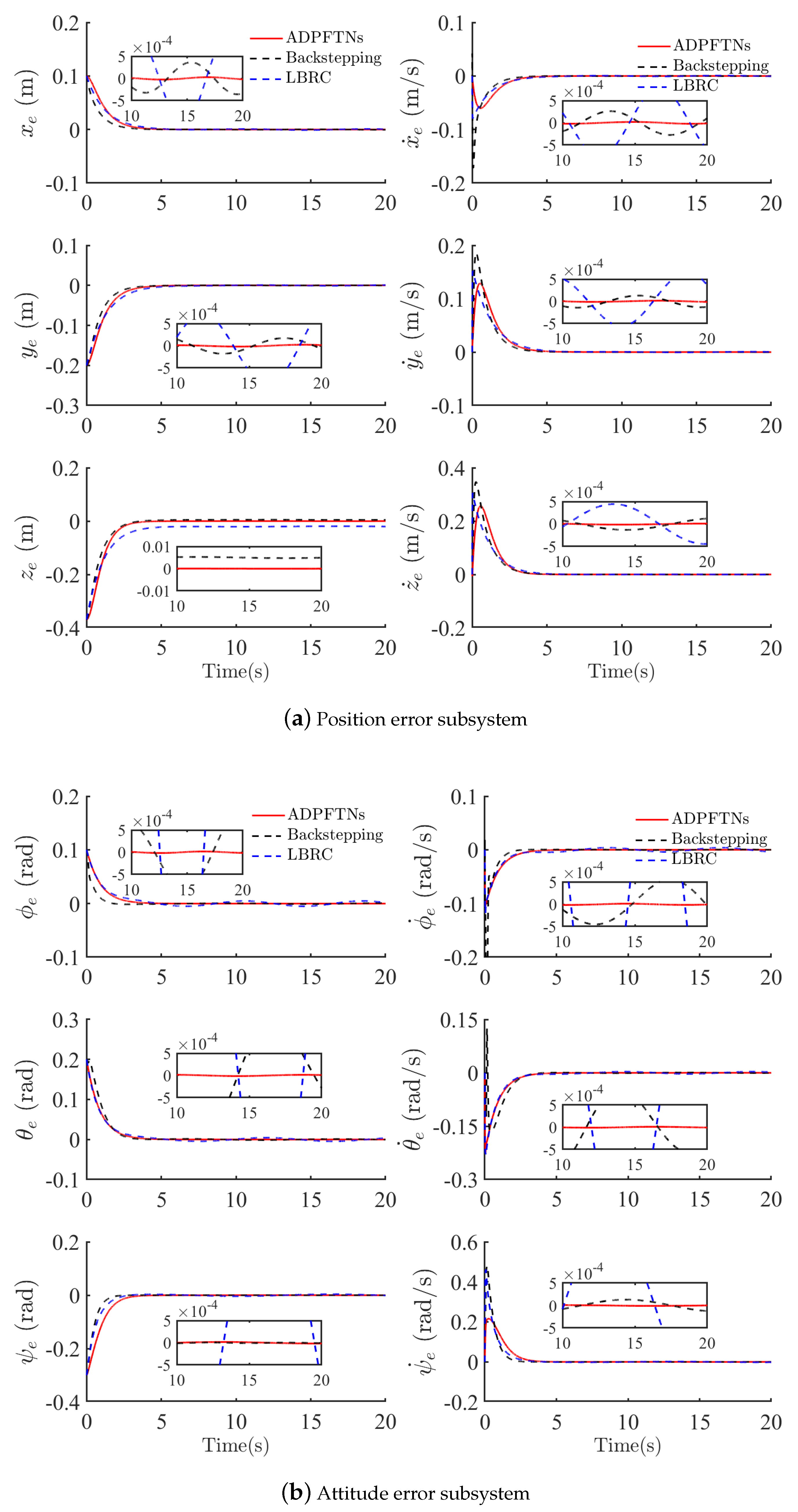
4.1. Robust Tracking Control Performances with Uncertainty

To highlight the superiority of the proposed ADPFTNs, the two NN-based observers (NNOBs) in [34] with the proposed approximate optimal control polices in (29) (denoted as ADPNNs) were employed to compare with the ADPFTNs. The uncertain parameter values were set as ${\Delta }_m=0.2+0.05·\mathrm{rand}\mathrm{kg},{\Delta }_{J_x}={\Delta }_{J_y}={\Delta }_{J_z}=0.03+0.01·\mathrm{rand}\mathrm{kg}·{\mathrm{m}}^2$, and ${\Delta }_{k_1}={\Delta }_{k_2}={\Delta }_{k_3}={\Delta }_{k_4}={\Delta }_{k_5}={\Delta }_{k_6}=0.005+0.001·\mathrm{rand}$. The $\mathrm{rand}$ function generates a random number in the interval $[0,1]$. ${\mathit{u}}_d={[0.1\sin \left(0.8t\right),0.1\sin \left(0.7t\right),0.1\sin \left(0.5t\right)]}^{\mathrm{T}}\mathrm{N}$ and ${\mathit{\tau }}_d={[0.1\sin \left(0.8t\right)+J_r\dot{\theta },0.1\sin \left(0.7t\right)-J_r\dot{\varphi },0.1\sin \left(0.5t\right)]}^{\mathrm{T}}\mathrm{N}·\mathrm{m}$ with $J_r\dot{\theta }$ and $J_r\dot{\varphi }$ being gyroscopic moments of the quadrotor UAV. The parameters of the ADPFTNs are given in

Table 1. Parameters’ selection.

Variable	Position Error System (i = 1)	Attitude Error System (i = 2)
$r_{i1}$	$1\times {10}^{-6}$	$1\times {10}^{-6}$
$r_{i2}$	$1\times {10}^{-5}$	$1\times {10}^{-5}$
$k_{i1}$	$0.01$	$0.01$
$k_{i2}$	$1.2$	$1.2$
${\mathit{Q}}_i$	$4{\mathit{I}}_6$	$10{\mathit{I}}_6$
${\mathit{R}}_i$	$2.5{\mathit{I}}_3$	$5{\mathit{I}}_3$
$r_{i3}$	$1.6$	$1.6$
$r_{i4}$	$0.2$	$0.2$
$c_i$	200	700
${\varrho }_{i1}$	$0.06$	$0.06$
$m_i$	97	99
$n_i$	99	101
$p_i$	105	105
$q_i$	99	101

.

Figure 3 shows the time response of the observation errors for the FTNNOBs and NNOBs, respectively. It can be observed that the observation error of the FTNNOBs stabilizes to the order of ${10}^{-4}$ within 0.5 s, while that of the NNOBs stabilizes to the order of ${10}^{-3}$ around 5 s. It can be concluded that the FTNNOBs have faster convergence performance and higher stabilization accuracy to attenuate external disturbances and parameter uncertainties in comparison with the NNOBs. Figure 4 shows the time response of the tracking errors for the ADPFTNs and the ADPNNs, respectively. For a fair comparison, we adjusted the convergence times of the two control schemes in the simulation to make them approximately equal (Section 4.2 performs the same setup). As shown in Figure 4, the tracking errors’ convergence curve of the proposed ADPFTNs is smoother than that of the ADPNNs and has higher convergence accuracy. This means that, when there are external disturbances and parameter uncertainties in the quadrotor UAV system, the FTNNOBs can quickly and accurately estimate the unknown uncertainties and compensate for the control policies. To illustrate the tracking performance of the two control schemes more directly, the 3D trajectory tracking results are shown in Figure 5. It can be observed that both the ADPFTNs and the ADPNNs can successfully track the desired trajectory. Further, it can be observed that the red solid line (the proposed ADPFTNs in this work) is more consistently close to the black solid line (desired trajectory) compared to the red dotted line (ADPNNs in [34]). Figure 6 shows the time responses of the AC NNs’ weights. One can see that the curves of the position error subsystem and attitude error subsystem stabilize after 5 s. Figure 7 shows the control inputs under the frame ${\mathit{\varsigma }}_E$.

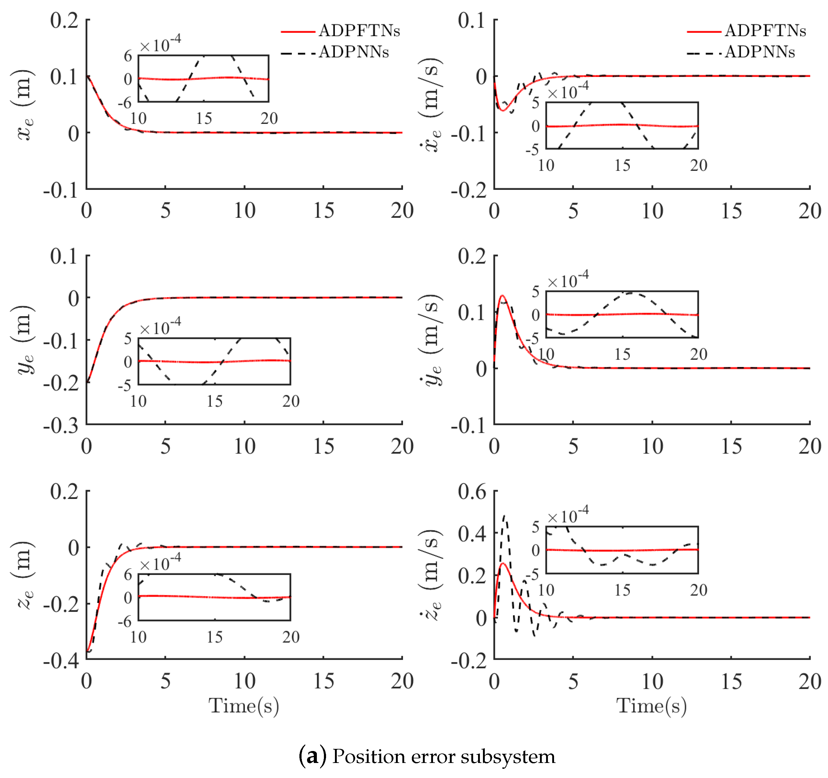
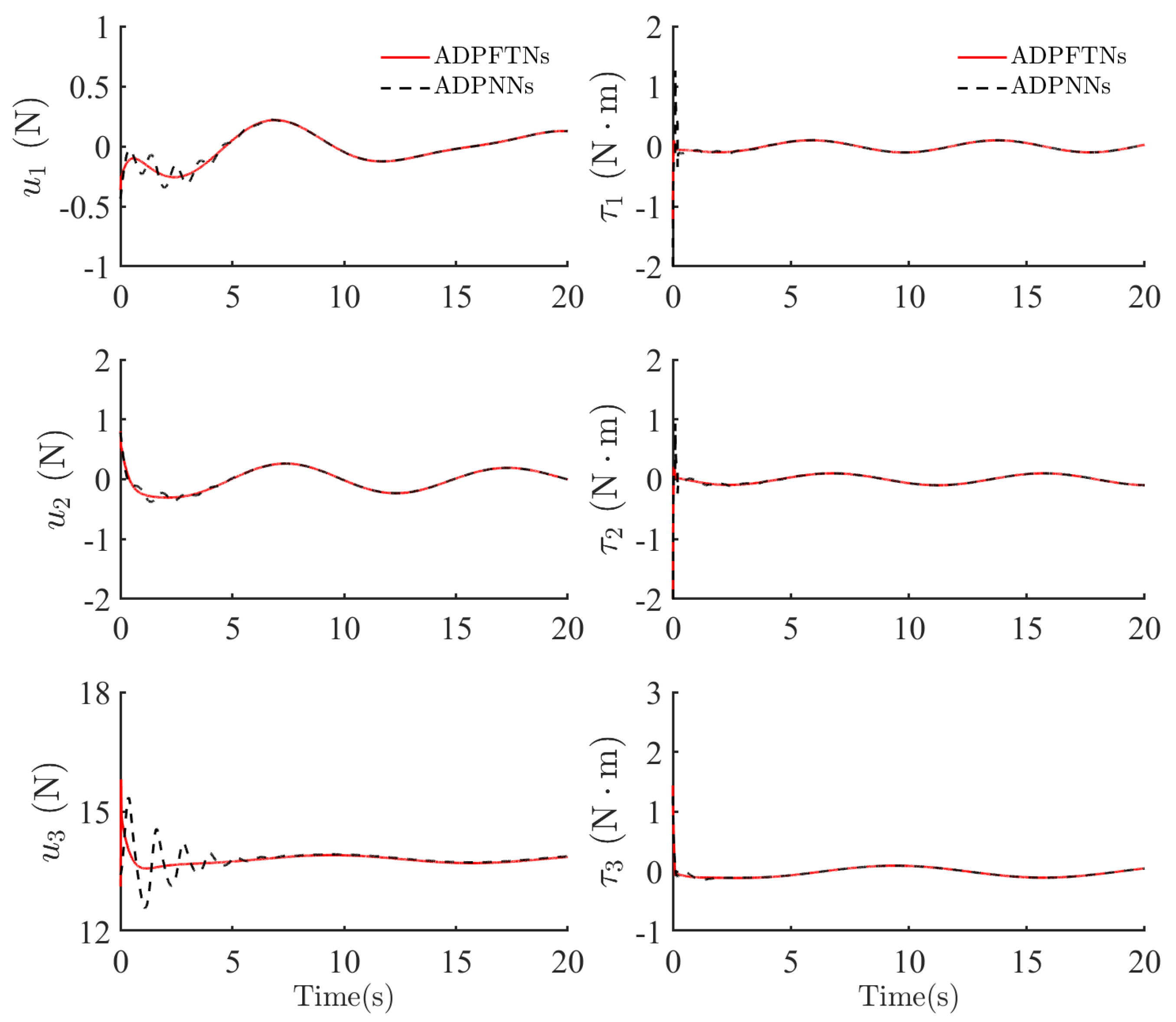
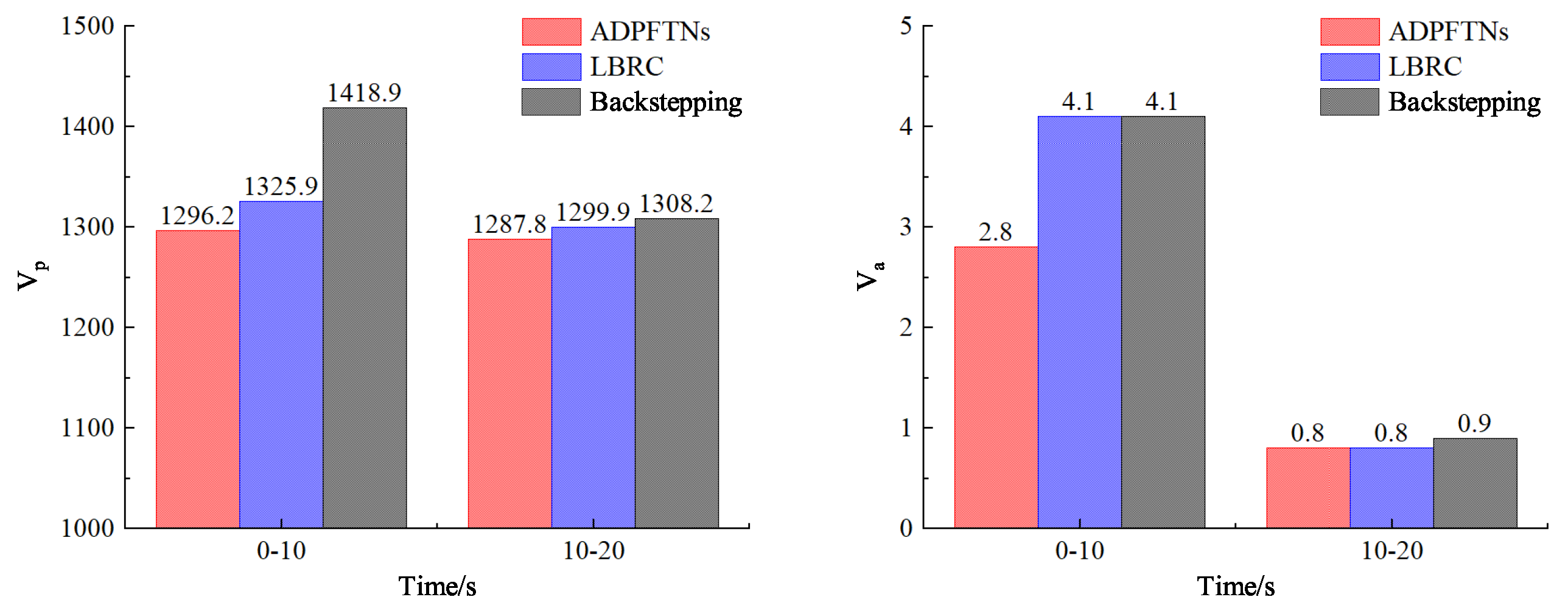
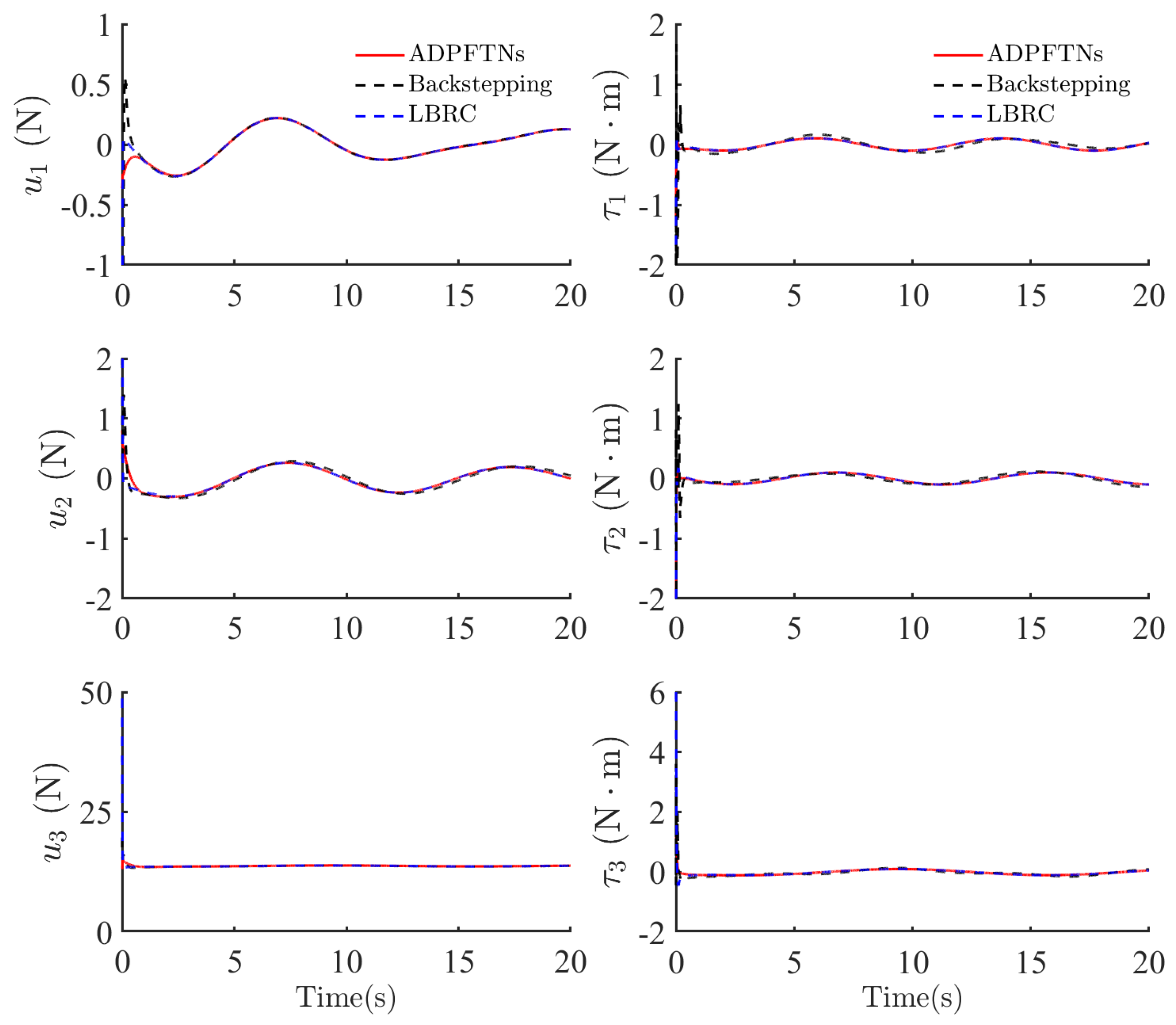
4.2. Tracking Control Performances and Cost

In this subsection, the control performances of the ADPFTNs in (19) are further analyzed from the perspective of control cost quantitatively and compared with the backstepping control scheme in [11] (denoted as Backstepping) and the learning-based robust control scheme in [50] (denoted as LBRC). For a fair comparison, the same cost functions are defined as ${\mathit{V}}_p={\int }_0^{\infty }({\mathit{e}}_1^{\mathrm{T}}{\mathit{Q}}_1{\mathit{e}}_1+{\mathit{u}}^{\mathrm{T}}{\mathit{R}}_1\mathit{u})$ and ${\mathit{V}}_a={\int }_0^{\infty }({\mathit{e}}_2^{\mathrm{T}}{\mathit{Q}}_2{\mathit{e}}_2+{\mathit{\tau }}^{\mathrm{T}}{\mathit{R}}_2\mathit{\tau })$, in which ${\mathit{V}}_p$ and ${\mathit{V}}_a$ represent the system of position and attitude control cost, respectively. For a convenient comparison of the position subsystem control cost, the gravity necessary for the three schemes was ignored in the calculation of the control cost ${\mathit{V}}_p$.

Figure 8 shows the time response of the tracking errors for the ADPFTNs, Backstepping, and LBRC, respectively. As shown in Figure 8, the stabilization accuracy of the ADPFTN was ${10}^{-5}$ orders of magnitude higher than the ${10}^{-4}$ orders of magnitude of Backstepping and LBRC in the same convergence time. In the convergence step, Backstepping and LBRC had steeper convergence trends and faster transient responses, while the ADPFTNs has a smooth convergence tendency. It is worth noting that the steep convergence trends and fast transient responses led to higher control cost. Figure 9 illustrates the control cost of the three control schemes. It can be observed that the ADPFTNs were capable of reducing the control cost while guaranteeing better control performances. In 0–10 s, the tracking errors lied in the convergence process, and it could be obtained that the ADPFTNs had lower control cost than Backstepping and LBRC, which demonstrates the superior performance of the ADPFTNs in reducing the control cost. After 10 s, the tracking error converged to a neighborhood of the origin, and there was no major difference in the control cost of the three control schemes. Compared to Backstepping, the total control cost of the position subsystem was reduced by $5.5\%$ and the total control cost of the attitude subsystem was reduced by $38.9\%$. In addition, the control inputs of the position system were larger than those of the attitude system, which accordingly led to a larger control cost of the position system. The 3D trajectory tracking results are illustrated in Figure 5. It can be observed that all three control schemes can successfully track the desired trajectory. Further, it can be seen that the red solid line had a more-stable tracking result in comparison with the blue dotted line (Backstepping in [11]) and the black dashed line (LBRC in [50]). Figure 10 shows the time response of control inputs in the frame ${\mathit{\varsigma }}_E$. As shown in Figure 9, the initial control inputs of the ADPFTNs were the smallest among the three schemes. Smaller control inputs had a smaller control cost, which corresponds to the results in Figure 9. This further illustrates the superiority of ADPFTNs in balancing control cost.

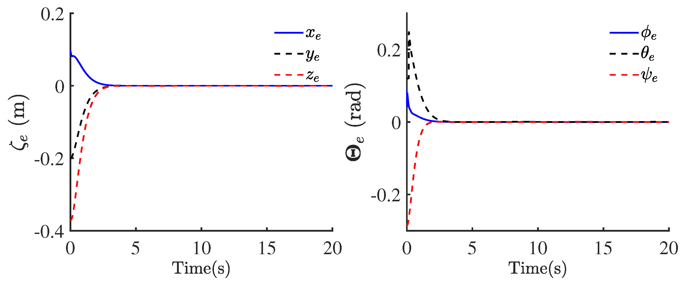
4.3. Matlab/Simscape Simulation Results

In this subsection, the effectiveness of the ADPFTNs is further validated by utilizing the semi-physical simulation environment of Matlab/Simscape, where the mathematical model was replaced with a 3D physical model of SolidWorks. The Quadrotor UAV 3D physical model parameters, external disturbances, and parameter uncertainties were set the same as in the numerical simulation section (Section 4.1 and Section 4.2). Figure 11 shows the time response of the tracking errors of the ADPFTNs in the Matlab/Simscape semi-physical simulation environment. It can be observed that all errors had good convergence performance. The control inputs of the semi-physical simulation are displayed in Figure 12. The simulation results of Matlab/Simscape semi-physical simulation environment in Figure 11 and Figure 12 were almost the same as the numerical simulation results, which indicated that the ADPFTNs have potential value to be extended and transplanted to engineering applications.

5. Conclusions

This paper investigated the ADP-based robust control problem of a quadrotor UAV trajectory tracking control system subject to external disturbances and parameter uncertainties. Firstly, the error subsystems were obtained by preprocessing the quadrotor UAV system using the feedforward technique. Subsequently, two FTNNOBs were designed to estimate external disturbances and parameter uncertainties quickly and accurately (observation errors converged within 0.5 s with an accuracy of the order of ${10}^{-4}$). Then, the AC NNs approximated the optimal value functions and the optimal control policies by designing two new weight update laws. Meanwhile, the designed weight update laws not only avoided utilizing the PE condition, but also improved the adaptive ability of the AC neural network. Finally, the ADPFTNs’ control scheme with high accuracy tracking performance (tracking accuracy of the order of ${10}^{-5}$) and low control cost (a total control cost of position subsystem savings of $5.5\%$; a total control cost of attitude subsystem savings of $38.9\%$) was proposed by combining the FTNNOBs and the approximate results of the AC NNs. Through Lyapunov stability analysis, the proposed control scheme can guarantee the closed-loop tracking control systems to be UUB stable. In the future, we will construct some experiments to demonstrate the practicability of the developed control scheme and perform some research on a multi-UAV system. Meanwhile, we will further improve the adopted model to enhance its accuracy and applicability to ensure that it better reflects the actual situation.

References

1. Liu, N.; Shao, X. Desired compensation RISE-based IBVS control of quadrotors for tracking a moving target. Nonlinear Dyn. 2019, 95, 2605–2624. [Google Scholar] [CrossRef]
2. Das, D.N.; Sewani, R.; Wang, J.; Tiwari, M.K. Synchronized truck and drone routing in package delivery logistics. IEEE Trans. Intell. Transp. Syst. 2021, 22, 5772–5782. [Google Scholar] [CrossRef]
3. Wu, Y.; Wu, S.B.; Hu, X.T. Cooperative path planning of UAVs & UGVs for a persistent surveillance task in urban environments. IEEE Internet Things J. 2021, 8, 4906–4919. [Google Scholar]
4. Gajbhiye, S.; Cabecinhas, D.; Silvestre, C.; Cunha, R. Geometric finite-time inner-outer loop trajectory tracking control strategy for quadrotor slung-load transportation. Nonlinear Dyn. 2022, 107, 2291–2308. [Google Scholar] [CrossRef]
5. Li, B.; Gong, W.Q.; Yang, Y.S.; Xiao, B. Distributed fixed-time leader-following formation control for multi-quadrotors with prescribed performance and collision avoidance. IEEE Trans. Aerosp. Electron. Syst. 2023, 59, 7281–7294. [Google Scholar] [CrossRef]
6. Labbadi, M.; Cherkaoui, M. Robust adaptive backstepping fast terminal sliding mode controller for uncertain quadrotor UAV. Aerosp. Sci. Technol. 2019, 93, 105306. [Google Scholar] [CrossRef]
7. Michael, N.; Mellinger, D.; Lindsey, Q.; Kumar, V. The GRASP Multiple Micro-UAV Testbed. IEEE Robot Autom. Mag. 2010, 17, 56–65. [Google Scholar] [CrossRef]
8. Sun, Y.B.; Xian, N.; Duan, H.B. Linear-quadratic regulator controller design for quadrotor based on pigeon-inspired optimization. Aircr. Eng. Aerosp. Tec. 2016, 88, 761–770. [Google Scholar] [CrossRef]
9. Li, B.; Gong, W.Q.; Yang, Y.S.; Xiao, B.; Ran, D.C. Appointed Fixed Time Observer-Based Sliding Mode Control for a Quadrotor UAV Under External Disturbances. IEEE Trans. Aerosp. Electron. Syst. 2022, 58, 290–303. [Google Scholar] [CrossRef]
10. Zhao, Z.; Cao, D.; Yang, J.; Wang, H. High-order sliding mode observer-based trajectory tracking control for a quadrotor UAV with uncertain dynamics. Nonlinear Dyn. 2020, 102, 2583–2596. [Google Scholar] [CrossRef]
11. Xiao, B.; Yin, S. A New Disturbance Attenuation Control Scheme for Quadrotor Unmanned Aerial Vehicles. IEEE Trans. Industr. Inform. 2017, 13, 2922–2932. [Google Scholar] [CrossRef]
12. Tran, V.P.; Santoso, F.; Garratt, M.A. Adaptive Trajectory Tracking for Quadrotor Systems in Unknown Wind Environments Using Particle Swarm Optimization-Based Strictly Negative Imaginary Controllers. IEEE Trans. Aerosp. Electron. Syst. 2021, 57, 1742–1752. [Google Scholar] [CrossRef]
13. Alifbek, K.K.; Stepan, D.; Murodbek, S.; Dmitry, A.P.; Anvari, G.; Javod, A. Expert system application for reactive power compensation in isolated electric power systems. Int. J. Electr. Comput. Eng. 2021, 11, 3682–3691. [Google Scholar]
14. Martyushev, N.V.; Malozyomov, B.V.; Khalikov, I.H.; Kukartsev, V.A.; Kukartsev, V.V.; Tynchenko, V.S.; Tynchenko, Y.A.; Qi, M. Review of Methods for Improving the Energy Efficiency of Electrified Ground Transport by Optimizing Battery Consumption. Energies 2023, 16, 729. [Google Scholar] [CrossRef]
15. Werbos, P.J. Consistency of HDP applied to a simple reinforcement learning problem. Neural Netw. 1990, 3, 179–189. [Google Scholar] [CrossRef]
16. Vamvoudakis, K.G.; Lewis, F.L. Online actor–Ccritic algorithm to solve the continuous-time infinite horizon optimal control problem. Automatica 2010, 46, 878–888. [Google Scholar] [CrossRef]
17. Kamalapurkar, R.; Dinh, H.; Bhasin, S.; Dixon, W.E. Approximate optimal trajectory tracking for continuous-time nonlinear systems. Automatica 2015, 51, 40–48. [Google Scholar] [CrossRef]
18. Wang, D.; Liu, D.R.; Li, H.L. Policy Iteration Algorithm for Online Design of Robust Control for a Class of Continuous-Time Nonlinear Systems. IEEE Trans. Autom. Sci. Eng. 2014, 11, 627–632. [Google Scholar] [CrossRef]
19. Wen, G.X.; Ge, S.S.; Tu, F.W. Optimized Backstepping for Tracking Control of Strict-Feedback Systems. IEEE Trans. Neural Netw. Learn. Syst. 2018, 29, 13. [Google Scholar]
20. Zhao, B.; Liu, D.R.; Li, Y.C. Observer based adaptive dynamic programming for fault tolerant control of a class of nonlinear systems. Inf. Sci. 2017, 384, 21–33. [Google Scholar] [CrossRef]
21. Wei, Q.L.; Liu, D.R.; Lin, Q.; Song, R.Z. Adaptive Dynamic Programming for Discrete-Time Zero-Sum Games. IEEE Trans. Neural Netw. Learn. Syst. 2018, 29, 957–969. [Google Scholar] [CrossRef]
22. Zhao, W.; Liu, H.; Lewis, F.L. Data-Driven Fault-Tolerant Control for Attitude Synchronization of Nonlinear Quadrotors. IEEE Trans. Automat. Control 2021, 66, 5584–5591. [Google Scholar] [CrossRef]
23. Chowdhary, G.; Yucelen, T.; Mühlegg, M.; Johnson, E.N. Concurrent learning adaptive control of linear systems with exponentially convergent bounds. Int. J. Adapt. Control Signal Process. 2013, 27, 280–301. [Google Scholar] [CrossRef]
24. Yang, X.; He, H. Self-learning robust optimal control for continuous-time nonlinear systems with mismatched disturbances. Neural Netw. 2018, 99, 19–30. [Google Scholar] [CrossRef] [PubMed]
25. Dong, H.Y.; Zhao, X.W.; Yang, H.Y. Reinforcement Learning-Based Approximate Optimal Control for Attitude Reorientation Under State Constraints. IEEE Trans. Control Syst. Technol. 2021, 29, 1664–1673. [Google Scholar] [CrossRef]
26. Liu, H.; Li, B.; Xiao, B.; Ran, D.C.; Zhang, C.X. Reinforcement learning© tracking control for a quadrotor unmanned aerial vehicle under external disturbances. Int. J. Robust Nonlinear Control. 2022, 33, 10360–10377. [Google Scholar] [CrossRef]
27. Sun, J.L.; Liu, C.S. Disturbance observer-based robust missile autopilot design with full-state constraints via adaptive dynamic programming. J. Frankl. Inst. 2018, 355, 2344–2368. [Google Scholar] [CrossRef]
28. Zhao, B.; Xu, S.Y.; Guo, J.Q.; Jiang, R.M.; Zhou, J. Integrated strapdown missile guidance and control based on neural network disturbance observer. Aerosp. Sci. Technol. 2019, 84, 170–181. [Google Scholar] [CrossRef]
29. Zhang, R.; Xu, B.; Shi, P. Finite time observer© output feedback control of MEMS gyroscopes with input saturation. Int. J. Robust Nonlinear Control. 2022, 32, 4300–4317. [Google Scholar] [CrossRef]
30. Zhao, Z.Y.; Jin, X.Z. Adaptive neural network-based sliding mode tracking control for agricultural quadrotor with variable payload. Comput. Electr. Eng. 2022, 103, 108336. [Google Scholar] [CrossRef]
31. Wang, D.D.; Zong, Q.; Tian, B.L.; Shao, S.K.; Zhang, X.Y.; Zhao, X.Y. Neural network disturbance observer-based distributed finite-time formation tracking control for multiple unmanned helicopters. ISA Trans. 2018, 73, 208–226. [Google Scholar] [CrossRef] [PubMed]
32. Liu, K.; Wang, R.J.; Wang, X.D.; Wang, X.X. Anti-saturation adaptive finite-time neural network based fault-tolerant tracking control for a quadrotor UAV with external disturbances. Aerosp. Sci. Technol. 2021, 115, 106790. [Google Scholar] [CrossRef]
33. Fan, Q.Y.; Yang, G.H. Adaptive Actor–Ccritic design-based integral sliding-mode control for partially unknown nonlinear systems with input disturbances. IEEE Trans. Neural Netw. Learn. Syst. 2016, 27, 165–177. [Google Scholar] [CrossRef] [PubMed]
34. Liu, X.; Zhao, B.; Liu, D.R. Fault tolerant tracking control for nonlinear systems with actuator failures through particle swarm optimization-based adaptive dynamic programming. Appl. Soft Comput. 2020, 97, 106766. [Google Scholar] [CrossRef]
35. Adhyaru, D.M. State observer design for nonlinear systems using neural network. Appl. Soft Comput. 2012, 12, 2530–2537. [Google Scholar] [CrossRef]
36. Farid, K.; Zhen Yu, Y.; Kenzo, N. Guidance and nonlinear control system for autonomous flight of minirotorcraft unmanned aerial vehicles. J. Field Robot. 2010, 27, 311–334. [Google Scholar]
37. Abeywardena, D.; Kodagoda, S.; Dissanayake, G.; Munasinghe, R. Improved State Estimation in Quadrotor MAVs: A Novel Drift-Free Velocity Estimator. IEEE Robot. Autom. Mag. 2013, 20, 32–39. [Google Scholar] [CrossRef]
38. Tang, P.; Zhang, F.B.; Ye, J.C.; Lin, D.F. An integral TSMC-based adaptive fault-tolerant control for quadrotor with external disturbances and parametric uncertainties. Aerosp. Sci. Technol. 2021, 109, 106415. [Google Scholar] [CrossRef]
39. Xiao, B.; Yin, S. Exponential Tracking Control of Robotic Manipulators With Uncertain Dynamics and Kinematics. IEEE Trans. Industr. Inform. 2019, 15, 689–698. [Google Scholar] [CrossRef]
40. Li, B.; Zhang, H.C.; Xiao, B.; Wang, C.H.; Yang, Y.S. Fixed-time integral sliding mode control of a high-order nonlinear system. Nonlinear Dyn. 2022, 107, 909–920. [Google Scholar] [CrossRef]
41. Zhao, L.; Yu, J.P.; Lin, C.; Yu, H.S. Distributed adaptive fixed-time consensus tracking for second-order multi-agent systems using modified terminal sliding mode. Appl. Math. Comput. 2017, 312, 23–35. [Google Scholar] [CrossRef]
42. Yu, S.H.; Yu, X.H.; Shirinzadeh, B.; Man, Z.H. Continuous finite-time control for robotic manipulators with terminal sliding mode. Automatica 2005, 41, 1957–1964. [Google Scholar] [CrossRef]
43. Shao, K.; Zheng, J.C.; Huang, K.; Wang, H.; Man, Z.H.; Fu, M.Y. Finite-time control of a linear motor positioner using adaptive recursive terminal sliding mode. IEEE Trans. Ind. Electron. 2020, 67, 6659–6668. [Google Scholar] [CrossRef]
44. Song, Y.D.; Huang, X.C.; Wen, C.Y. Tracking Control for a Class of Unknown Nonsquare MIMO Nonaffine Systems: A Deep-Rooted Information Based Robust Adaptive Approach. IEEE Trans. Automat. Control 2016, 61, 3227–3233. [Google Scholar] [CrossRef]
45. Hornik, K.; Stinchcombe, M.; White, H. Multilayer feedforward networks are universal approximators. Neural Netw. 1989, 2, 359–366. [Google Scholar] [CrossRef]
46. Girosi, F.; Poggio, T. Networks and the best approximation property. Biol. Cybern. 1990, 63, 169–176. [Google Scholar] [CrossRef]
47. Zhang, D.H.; Kong, L.H.; Zhang, S.; Li, Q.; Fu, Q. Neural networks-based fixed-time control for a robot with uncertainties and input deadzone. Neurocomputing 2020, 390, 139–147. [Google Scholar] [CrossRef]
48. Wen, G.X.; Chen, C.L.P.; Ge, S.S. Simplified Optimized Backstepping Control for a Class of Nonlinear Strict-Feedback Systems With Unknown Dynamic Functions. IEEE Trans. Cybern. 2021, 51, 4567–4580. [Google Scholar] [CrossRef]
49. Li, K.W.; Li, Y.M. Adaptive NN optimal consensus fault-tolerant control for stochastic nonlinear multiagent systems. IEEE Trans. Neural Netw. Learn. Syst. 2021, 34, 947–957. [Google Scholar] [CrossRef]
50. Mu, C.X.; Zhang, Y. Learning-Based Robust Tracking Control of Quadrotor With Time-Varying and Coupling Uncertainties. IEEE Trans. Neural Netw. Learn. Syst. 2020, 31, 259–273. [Google Scholar] [CrossRef]
Figure 1. Mechanical structure of a quadrotor UAV.
Applsci 13 12672 g001
Figure 2. Framework for ADP-based robust tracking control of the quadrotor UAV system.
Applsci 13 12672 g002
Figure 3. Time response of the observation errors by different observers.
Applsci 13 12672 g003
Figure 4. Time response of tracking errors under ADPFTNs and ADPNNs.
Applsci 13 12672 g004aApplsci 13 12672 g004b
Figure 5. Three-dimensional trajectory tracking results under different control schemes.
Applsci 13 12672 g005
Figure 6. Time responses of AC NNs’ weights of ADPFTNs.
Applsci 13 12672 g006
Figure 7. Time response of control inputs under ADPFTNs and ADPNNs.
Applsci 13 12672 g007
Figure 8. Time response of tracking errors under different schemes.
Applsci 13 12672 g008
Figure 9. The position control cost and attitude control cost under different schemes.
Applsci 13 12672 g009
Figure 10. Time responses of control inputs under different schemes.
Applsci 13 12672 g010
Figure 11. Time response of tracking errors of ADPFTNs in Simscape.
Applsci 13 12672 g011
Figure 12. Time response of control inputs of ADPFTNs in Simscape.
Applsci 13 12672 g012