Abstract
Despite having some fluctuations and the impact of the COVID-19 crisis, the demand for flights had a general growing trend for the past years. As the airspace is limited, efforts to better manage the total number of flights are noteworthy. In addition, volatility (i.e., unpredicted changes) in the number of flights has been observed to be increasing. Efforts to improve flight forecasting are thus necessary to improve air traffic efficiency and reduce costs. In this study, volatility in the number of flights is estimated based on past trends, and the outcomes are used to project future levels. This enables risk situations such as having to manage unexpectedly high numbers of flights to be predicted. The methodological approach analyses the Functional Airspace Block of Central Europe (FABEC). Based on the number of flights for 2015–2019, the following are calculated: historic mean, variance, volatility, 95th percentile, flights per hour and flights per day of the week in different time zones in six countries. Due to the nature of air traffic and the overdispersion observed, this study uses counting data models such as negative binomial regressions. This makes it possible to calculate risk measures including expected shortfall (ES) and value at risk (VaR), showing for each hour that the number of flights can exceed planned levels by a certain number. The study finds that in Germany and Belgium at 13:00 h there is a 5% worst-case possibility of having averages of 683 and 246 flights, respectively. The method proposed is useful for planning under uncertainties. It is conducive to efficient airspace management, so risk indicators help Air Navigation Service Providers (ANSPs) to plan for low-probability situations in which there may be large numbers of flights.
1. Introduction
Due to the growing number of flights, increasing delays and high-cost pressure on the whole aviation system, the provision of Air Navigation Services (ANS) has recently drawn increasing attention from both academics and policy decision-makers. A major challenge regarding ANS provision is “planning under uncertainties”, e.g., as a result of volatile traffic demand in terms of movement numbers and flow patterns, which can significantly influence resource planning and allocation. Several factors could cause or increase volatility, e.g., weather, strikes, geopolitical factors, airline decisions and unexpected economic downturns [1].
Volatile traffic affects ANS planning on multiple time scales and operational levels [2]. Changes in traffic demand and flow patterns have a direct influence on pre-tactical and strategic capacity planning and on resulting delays, their associated costs and safety. Thus, traffic volatility and the associated airspace risk have become a daily concern for Europe’s ANSPs and Functional Airspace Blocks (FABs), posing a complex challenge due to the size and extent of the problem. So much so that FABEC launched an interactive platform in 2018 to discuss this topic as part of an initiative addressing new developments in air traffic flow management. In the aftermath of the COVID-19 pandemic, the importance of addressing this issue has become even clearer: Although traffic in FABEC started to recover in 2021, the increase in demand was slow and accompanied by extreme volatility, as unplanned flights put pressure on airspace capacity and staff resources.
Changes in traffic demand are not a new phenomenon. But there are at least two reasons that explain why this issue is taken seriously and why a more in-depth analysis of its causes and consequences is being undertaken [3]. On the one hand, volatility has shifted from being an isolated phenomenon to affecting the entire aviation system. On the other hand, recent years have been characterised by increasingly wide variations in the volume of flights and routes (and a high level of volatility in the rate of recovery of traffic levels across Europe following the COVID-19 pandemic).
Figure 1 shows changes in air traffic relative to the base year of 1970 for different countries. Note that, in all cases, the tendency is for a steady increase as years go by. Surprisingly, in 2019, air traffic fell just prior to the general spread of the COVID-19 pandemic. COVID-19 affected the mobility of European air transport with a reduction of as much as 89% in the number of flights [4] and created an uncertain future for the aviation industry [5]. In any event, it must be noted that, in general, the air traffic pattern shows tremendous changes, mean reversion and jumps.
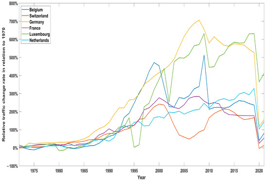
Figure 1.
Rate of change in air traffic relative to 1970. Source: Prepared by authors using data from ref. [6].
ANSPs are constantly recruiting new personnel (controllers) and adapting capacity to demand to provide more flexibility. These solutions have proved effective in the short term [7], but as activity in the industry becomes even more unpredictable [8,9], it is increasingly clear that new ways of setting targets, assessing performance plans in terms of profitability and ultimately measuring the impact of volatility on ANSP operations need to be found. Providing flexible air traffic services therefore requires new thinking to minimise the impact of volatility on the travelling public, while at the same time providing the capacity to meet demand in the short- and long term. This means that efforts to understand what volatility is and propose ways to measure and estimate it are especially welcome in this topic.
The complexity and scope of the industry offer a number of research opportunities from a variety of perspectives. For example, studies on volatility have focused on applying a few metrics [10] or [11] realise a survey on Artificial Intelligence (AI) in order to maintain aviation safety. In the analysis of air traffic flows and delays, there is one part that can be predicted (deterministic) and another that cannot (stochastic). It is common to focus only on the deterministic part. However, when it comes to the aviation sector, non-predictable information (strikes, weather, etc.) is even more important than in other sectors. The study by [12] focuses on volatility (and on changes in it) by applying a stochastic modelling method to estimate future air traffic, delays and the cost of future delays in Germany to quantify risk and its significance for the delivery of cost-effective services.
In this study, we propose negative binomial regression models as a way of estimating volatility in the number of flights in the FABEC area, which compromises the airspace of France, Benelux, Germany and Switzerland and is regarded as the core area of Europe. By estimating the necessary parameters, we can obtain the volatility in the number of flights depending on the days of the week and the hours. That is, we propose a method for reducing and using the uncertainty associated with the number of flights per hour so as to contribute to better planning of ANS. We use hourly traffic data for 2015–2019.
As far as we know, this is a novel methodology that has never before been applied for estimating volatility in the aviation sector. By estimating volatility parameters, we are able to draw up simulations that reveal the full distribution of the number of flights for all FABEC countries. The distributions are very useful in understanding the likelihood and risk of the number of flights exceeding a given threshold number.
The paper is structured as follows: Section 2 reviews the literature and presents the approach. Section 3 provides the data used for the analysis. Section 4 sets out the counting data model, which is a negative binomial regression model. Results and conclusions are given in Section 5 and Section 6, respectively.
2. State of the Art
Air Traffic Management (ATM) needs to be improved in the wake of significant growth and variations in traffic [13]. A new regulatory framework could enhance safety, cost and flight efficiency; an elastic economic regulatory system could also enable capacity and react faster to changes in demand. Such a new ATM system would enhance the Green Deal measures [14].
Single European Sky ATM Research (SESAR) was created in 2008 due to increasing air traffic and rational delays since 2000. Its fourth pillar establishes the management of air transport capacity. In 2018, the Airspace Architecture Study (AAS) [15] identified possible solutions for capacity and demand imbalance such as arrival management and improved aviation meteorology. In [16], two main challenges in the Main Plan (MP) are foreseen: environmental concerns and a mismatch between traffic demand and ATM capacity.
Delays can be due to various reasons including weather conditions [17], ground delays, runway queues and capacity constraints [18], and delays are a major source of direct and opportunity costs [19]. A review of different approaches to flight delay prediction and how this problem is addressed is presented in [20]. They compare the prediction models used, such as operational research [21], machine learning [22], Bayesian network approach [23], probabilistic models, statistical analysis, a super statistical approach [24] and ensemble methods and select representative algorithms [25]. A novel predictive model applying graphs to sequence learning architecture is studied in [26]. Authors in [27] affirm that comparing flight schedules and flight plans is a very useful way of locating flight delay occurrences and modelling flight delays.
Air traffic network efficiency depends on strikes [28] and arrival processes [29] among other factors. The Arrival Manager (AMAN) seeks to improve the flow when capacity constraints exist, so the system needs reliable assessment and estimations of delay and capacity. All this translates into additional miles flown due to cancellations, delays or rerouting of scheduled flights, increasing horizontal flight distance and thus affecting fuel consumption, environmental factors and costs to customers and airlines [30]. An analysis of the insights on the estimated climate costs of the aviation sector due to air management for 2018 and 2019 is presented in [31] and found them to be as high as 1 bn EUR. Other authors study the expected costs for airspace users as a result of Air Traffic Management (ATFM) regulations [32].
ANSPs, airlines, planners and regulators manage imbalances between short- and long-term demand and air capacity in different FABs. Recently, the Eurocontrol Network Operations Plan (NOP) realised that traffic flow predictions are not as accurate as they used to be because of sharp peaks in demand, which make it difficult to apply enough capacity. This situation is exacerbated in core areas of Europe such as FABEC, where 60% of airlines are flying longer and more expensively [2]. As a result, a new term has become very familiar in ATM: volatility. This refers to unexpected changes in the number of flights. It seems to be a useful indicator that can further understanding of the balance between demand and capacity, i.e., traffic variations in time and space. Volatility depends on seasonality, weather forecasts, the closing of airspace due to geopolitical decisions, strikes, airline decisions, unexpected Air Traffic Charges (ATC), service charges and economic cycles. A fuzzy cognitive map of 39 concepts to analyse the links between them and estimate the causes and effects of volatility is drawn in [1]. Guerra et al. conducted a literature review of volatility in air transport, identified factors that influence it and suggested strategies for addressing it [33]. However, they do not mention volatility as a measure of flight fluctuation. The reference [34] shows that the path and cycle approach is a reasonable way of modelling this hotspot problem.
Volatility seems to be an emerging topic in ATM and one that affects Air Space Management (ASM), planning, air security, environmental issues and airport management. The literature mentions various topics directly and indirectly affected by flight volatility such as the foregoing, but as far as we are aware, there is no clear definition of the concept of “volatility in a number of flights” and therefore, no clearly identified model for predicting such volatility.
3. Materials: The Data
In the current study, volatility means a fluctuation in output, not in resources. In terms of ANSPs, output includes metrics, e.g., flight hours, flights, movements at airports and flight distances. So in this case, we are particularly interested in variations in the number of flights.
Eurocontrol offers a number of public and semi-public data sources, e.g., the ATM Cost-Effectiveness (ACE) data [35] and Performance Review Unit (PRU) data [36]. However, each of these datasets covers different temporal and operational levels. They also differ in regard to the years available. The key criterion for this study is the granularity of the data. Data on a daily basis is not sufficient to address short-term volatility, so the PRU database cannot be used. However, there is no publicly available data source for hourly flights. As an alternative, however, ANSPs have access to trajectory data, which can be analysed, for example, via the Network Strategic Tool (NEST) [37]. NEST provides both the actual and planned numbers of flights.
The dataset used for short-term volatility was obtained by using a NEST assessment [38]. Hourly data are available for 2015–2019. Overall, the dataset contains 89 units. However, airspaces often contain overlapping areas. For example, the airspace ED contains all areas connoted to Germany, including parts of Maastricht UAC. However, flights are also available for EDCC (German Area Control Centres (ACCs)) and EDYYCC (Maastricht ACC in German airspace). Finally, there are units with a “CTA” suffix, so the _CC and _CTA airspaces may be subsets, but this is not the case for all observations. As a result, the database was split up in advance to avoid double counting. The differences between LP and LPCC airspace are illustrated in Figure 2.
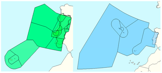
Figure 2.
Portuguese airspace according to NEST—LP (left) and LPCC (right).
The times indicated are in UTC/GMT and refer to the time stamp when a flight enters the unit.
Note that the accuracy of these data is limited in 3 dimensions: time (1 min), vertical distance (400 ft) (or 1000 ft in the climb/descent-phase) and lateral distance (10 NM).
A preliminary analysis of the actual data presented in Table 1, Table 2 and Table 3 shows a clear overdispersion in many hour ranges. That is, the variance is well above the mean in all cases. Data for Germany are used to illustrate the analysis, but the comments and findings can be generalised to all FABEC countries, as shown below.

Table 1.
Historic mean, variance and risk for Germany (EDCC) depending on the hour.
Table 2.
Mean number of flights in Germany depending on day of the week.
Table 3.
Historic mean, variance and risk for FABEC countries between 9 and 12 h.
Note that the variance depends on the time of the flight (from 1–24 h), with 10 h being the time when traffic is heaviest. However, a look at the 95th percentile shows that the highest risk occurs at 9 h, given that there are more than 715 flights in 5% of cases.
Table 1 also shows that there are big differences between volatility and the variance/mean ratio depending on the hour. Note that neither variance nor volatility values take into consideration whether the values on the database are high or low, but the ratio does take this into consideration. This is why the use of the ratio is recommended. However, from the point of view of airspace saturation, more attention must be paid to volatility during peak traffic hours, i.e., when the 95th percentile shows high values, because in such situations the risk of saturation is much higher.
Table 2 presents the mean air traffic figures per hour and per day of the week in Germany. It illustrates that time and day of the week patterns may exist, such as substantial increases in flights between 6 h and 19:00 h. Big differences may arise between different days of the week.
Table 3 shows some data indicators for all the countries in the FABEC area for times from 9:00 to 12:00. These are the hours with the greatest air traffic for all these countries except Belgium, where the peak is at 16 h. A clear overdispersion can be noted.
4. Methods: Modelling Efforts and Calibration
When there is a need to model a variable such as air traffic, which takes integer or zero values, the use of counting data models seems appropriate [39,40,41]. These are specific models for situations in which the dependent variable is either integer positive or zero, i.e., it cannot, by nature, have a negative sign. In such cases, variance is a function of the expected value. In this specific case, the expected value depends on the time, day of the week, seasonality and trend.
The most widely used counting regression models are the Poisson and the negative binomial. Using these models, highly accurate forecasts can be made of the expected number of events (number of flights in this case) and of volatility. In this case, volatility is caused by the uncertainty in the number of flights in each hour. For instance, some authors [42] have used the lineal Poison autoregressive (PAR) model as an alternative to the Poisson model to analyse the impacts of laws and climate on annual road traffic accidents. This alternative method may be applied in future work for comparative purposes.
Note that in the Poisson model, the variance is equal to the expected value, which has its limitations. However, the negative binomial model is applied in situations in which there is overdispersion, i.e., when the variance is greater than the mean. Therefore, an initial analysis of the data is required before it can be decided which of the two models fits better for the purpose of this paper, although there are more precise statistics for making this decision. The preliminary data analysis in Section 3 suggests that a negative binomial model is more adequate for analysing air traffic.
This model is an extension of Poisson regression for cases in which the variance is greater than the mean value. As stated, this is the case of the data used here.
In a counting regression model such as the negative binomial, the expected value is as shown in Equation (1).
where Y stands for the number of flights and X represents the independent variables. The calculation of expected value includes:
- (a)
- A constant .
- (b)
- A trend where t is the time in years.
- (c)
- A yearly cycle with its seasonal components: annual, semi-annual, quarterly, etc.
- (d)
- A weekly cycle depending on the days of the week. These are dummy variables.
- (e)
- A daily cycle based on the hours with their seasonal components in a similar way to the yearly cycle.
The yearly cycle is modelled as in Equation (2).
The weekly cycle is modelled as in Equation (3) using six dummy variables.
where the dummy variable if the day is Monday and for other days of the week. When all dummy variables are zero, it is Sunday.
The hourly cycle is modelled as in Equation (4).
where the variable τ indicates the hour and takes a value between 1 and 24. There are 28 parameters for calculating the expected value in the overall model, depending on trend, annual cycle, weekday and time. Table 4 presents the parameter values calculated for Germany, where the betas correspond to the constant, trend, yearly cycle parameters, weekly parameters and daily cycle parameters as specified in Equation (1) to Equation (4), also the alpha value is calculated.
Table 4.
Negative binomial parameters for Germany.
In this regression model, the variance is calculated using Equation (5).
where α is a value calculated by the regression. Figure 3 shows the variance values as functions of α and μ.
Var(Y|X) = (1 + α × μ) × μ
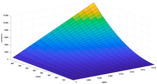
Figure 3.
The variance values as functions of α and μ.
The value of parameter α is obtained by regressing the model in Equation (1). The calculation process can be found in text books as given in [41].
With E(Y|X) = the variance can be obtained using Equation (5). These estimates enable future numbers of flights to be simulated and the full distribution to be obtained. Risk measures can then be proposed to cater for situations in which a given number of flights might be exceeded.
The measures of risk calculated are the well-known ES and VaR [43]. The VaR (95%) is the 95th percentile and is the number of flights that is only exceeded in 5% of cases. This is usually estimated for the 95% percentile, which illustrates the exact point above which the low probability (5%) zone of having an unmanageable number of flights is entered. The ES shows the mean number of flights in that zone or for the 5% of worst cases. Both risk measures are employed to better understand what may happen in the unfavourable tail of the distribution. This is why both ES and VaR are used as risk measures under uncertain conditions.
The method also enables correlations to be estimated between numbers of flights in different countries so as to provide an understanding of the links between different airspaces, so it can be used to develop new airspace regulations.
5. Results and Discussion
The method proposed enables us to estimate the alpha values, which can be shown here as indicators of volatility. The higher these parameters are, the higher the volatility is. As explained above, once the value for alpha is obtained, it is easy to run simulations and obtain the full distribution of the number of flights per hour and per country analysed. In addition, correlations can be estimated between the numbers of flights in different countries in an effort to better understand the interrelationship of airspaces at given times.
For the following calculations, Equation (6) is used. This is a reduced version of Equation (1), where the weekly cycle is erased and calculations are performed per hour. This enables an alpha value to be calculated for each hour and country. However, note that the method proposed can be used with a higher level of disaggregation for each country, hour and day of the week and even for other time periods such as months.
Table 5 presents the values for Belgium as an illustration. The values for the other countries are shown in Appendix A. These variables for some hours are not statistically different from zero, which usually happens when the alpha value is small. Note that when alpha is zero, we are in the case of Poisson regression as there is no overdispersion. The Poisson model is nested in the negative binomial model.
Table 5.
Alpha values for Belgium.
To calculate risk indicators, an expected figure must first be calculated, and then, the full distributions of flights must be obtained. There are various ways of estimating the expected value. In this paper, we use Equation (1) for a given day, i.e., 15 December 2023. Any other day could be used for this purpose, or expected values could be estimated by other methods. Once the expected value is calculated for a given time and day, we use the estimated alpha values to obtain the variance by applying Equation (5). Note that variance is defined as the square of volatility.
Table 6 presents the 95th percentile risk measures and the ES (95%) (i.e., the mean of the 5% of worst cases) for each hour and country. These risk measures are calculated using negative binomial simulations for 1,000,000 values. A mean of simulated values is shown in each case to control for the correct execution of the simulation.
Table 6.
Risk measures.
The values above show that in the cases of Germany and Belgium, for instance, there is a 5% chance of average numbers of flights being 683 and 246 at 13:00 h. Knowing these risk indicators can help the authorities to plan for low-probability situations in which large numbers of flights may arise. Being prepared for low-probability, high-impact situations is tantamount to good risk-averse planning.
6. Conclusions
Volatility in the number of flights poses a serious challenge to airspace management in all countries in the FABEC area. Every year, great efforts are put into trying to understand this and learning to anticipate how the number of flights may fluctuate at given times and on given days of the year.
The analysis presented in this paper presents a sound mathematical method for estimating volatility in the near future based on past data. This volatility may differ depending on various factors, such as country, time and day of the week. This estimation effort then makes it possible to obtain the full distribution of expected flights at a given future time and, consequently, to estimate risk indicators in the form of ES and VaR. These indicators highlight situations in which the number of flights may exceed a given threshold and come to pose a risk for anyone who has to manage the airspace.
The method is applied using actual data to estimate expected future flight numbers and volatilities for each period of interest in each country. Using the expected flights and variance calculated, the full distributions are obtained for those periods and the risk measures are calculated. As far as we know, this is the first time this method has been applied to estimate the volatility of the number of flights, taking into account that the number must be an integer or zero and that volatility can vary with certain factors such as the time and day of the week. The results shown here should enable airspace to be managed in a safer, economically optimal fashion.
The method proposed can also be applied in three other ways:
- (a)
- By combining different methods to estimate expected flights and using the methodology presented here to estimate volatility and risk measures.
- (b)
- By using a higher level of disaggregation in time periods such as months combined with minutes, hours and days of the week.
- (c)
- By linking volatility and risk with welfare, employment and CO2 emissions.
Availability of data and the possibility of making those data public are thus the only limiting factors in undertaking a much more in-depth, detailed analysis.
Author Contributions
Conceptualisation, I.G., L.M.A., T.S., I.R.d.G. and N.G.; methodology, I.G. and L.M.A.; software, L.M.A.; validation, I.G. and T.S.; formal analysis, L.M.A., I.R.d.G. and N.G.; investigation, I.G., L.M.A. and T.S.; resources, T.S.; data curation, I.G., L.M.A. and I.R.d.G.; writing—original draft preparation, I.G., L.M.A. and N.G.; writing—review and editing, T.S. and N.G.; visualisation, L.M.A., T.S. and I.R.d.G.; supervision, I.G. and T.S.; funding acquisition, I.G. and N.G. All authors have read and agreed to the published version of the manuscript.
Funding
This research is supported by María de Maeztu Excellence Unit 2020–2027 Ref. CEX2021-001201-M, funded by MCIN/AEI/10.13039/501100011033. Further support is provided by the Spanish Ministry of Science, Innovation and Universities (MINECO) (Grant RTI-2018-093352-B-I00). Ibon Galarraga and Nestor Goicoechea are grateful for financial support from Research Group B at the University of the Basque Country (Ref. IT1777-22).
Institutional Review Board Statement
Not applicable.
Informed Consent Statement
Not applicable.
Data Availability Statement
The data presented in this study are available on request from the corresponding author. The data are not publicly available due to restrictions from the data owner.
Conflicts of Interest
The authors declare that they have no known competing financial interests or personal relationships that could have appeared to influence the work reported in this paper.
Nomenclature
| Abbreviations: | |
| AAS | Airspace Architecture Study |
| ACCs | Area Control Centres |
| ACE | ATM Cost-Effectiveness |
| AI | Artificial Intelligence |
| AMAN | Arrival Manager |
| ANS | Air Navigation Services |
| ANSP | Air Navigation Service Providers |
| ASM | Air Space Management |
| ATC | Air Traffic Charges |
| ATFM | Air Traffic Flow Management |
| ATM | Air Traffic Management |
| COVID-19 | Corona virus 2019 |
| CTA | Controlled airspace |
| ED | All areas connoted to Germany |
| EDCC | German Area Control Centres |
| EDYYYC | Maastricht ACC in German Space |
| ES | Expected shortfall |
| FAB | Functional Airspace Block |
| FABEC | Functional Airspace Block Central Europe |
| GMT | Greenwich Mean Time |
| LP | All areas connoted to Portugal |
| MP | Main Plan |
| NEST | Network Strategic Tool |
| NM | Nautical Mile |
| NOP | Network Operation Plan |
| PRU | Performance Review Unit |
| SESAR | Single European Sky ATM Research |
| UAC | Upper Area Control |
| UTC | Universal Coordinated Time |
| VaR | Value at Risk |
| Counting model variables and parameters: | |
| Expected number of flights | |
| Y | Number of flights |
| X | Independent variables |
| Negative binomial parameters | |
| Yearly cycle | |
| Weekly cycle | |
| Daily cycle | |
| Dummy variables | |
| τ | Hour values between 1 and 24 |
| QML | Quasi Maximum Likelihood |
Appendix A
All Tables in Appendix A show the authors’ own calculations.
Table A1.
Alpha values for Belgium.
Table A1.
Alpha values for Belgium.
| Hour | Alpha Value | Standard Deviation | z | p-Value | |
|---|---|---|---|---|---|
| 9 | 0.002131 | 0.000939 | 2.2690 | 0.0233 | ** |
| 10 | 0.000636 | 0.000704 | 0.9029 | 0.3666 | |
| 11 | 0.001390 | 0.000762 | 1.8240 | 0.0681 | * |
| 12 | 0.000833 | 0.000638 | 1.3040 | 0.1922 | |
| 13 | 0.000550 | 0.000542 | 1.0150 | 0.3101 | |
| 14 | 0.001786 | 0.000434 | 4.1120 | 0.0000 | *** |
| 15 | 0.000973 | 0.000340 | 2.8630 | 0.0042 | *** |
| 16 | 0.001247 | 0.000309 | 4.0320 | 0.0001 | *** |
Note: Asterisks denote significance as follows: *** 0.1% level; ** 1%; * 5%.
Table A2.
Alpha values for Germany.
Table A2.
Alpha values for Germany.
| Hour | Alpha Value | Standard Deviation | z | p-Value | |
|---|---|---|---|---|---|
| 9 | 0.004061 | 0.001554 | 2.6130 | 0.0090 | *** |
| 10 | 0.002289 | 0.001170 | 1.9570 | 0.0504 | * |
| 11 | 0.002441 | 0.001143 | 2.1350 | 0.0328 | ** |
| 12 | 0.002760 | 0.000892 | 3.0950 | 0.0020 | *** |
| 13 | 0.001910 | 0.000652 | 2.9280 | 0.0034 | *** |
| 14 | 0.002354 | 0.000469 | 5.0200 | 0.0000 | *** |
| 15 | 0.001920 | 0.000297 | 6.4700 | 0.0000 | *** |
| 16 | 0.003658 | 0.000192 | 19.0700 | 0.0000 | *** |
Note: Asterisks denote significance as follows: *** 0.1% level; ** 1%; * 5%.
Table A3.
Alpha values for the Netherlands.
Table A3.
Alpha values for the Netherlands.
| Hour | Alpha Value | Standard Deviation | z | p-Value | |
|---|---|---|---|---|---|
| 9 | 0.001006 | 0.000831 | 1.2110 | 0.2258 | |
| 10 | 0.001083 | 0.000759 | 1.4270 | 0.1536 | |
| 11 | 0.001936 | 0.000889 | 2.1780 | 0.0294 | ** |
| 12 | 0.000917 | 0.000633 | 1.4480 | 0.1475 | |
| 13 | 0.000384 | 0.000531 | 0.7226 | 0.4699 | |
| 14 | 0.000000 | Poisson | |||
| 15 | 0.000000 | 0.000172 | 0.0003 | 0.9998 | |
| 16 | 0.000689 | 0.000377 | 1.8300 | 0.0673 | * |
Note: Asterisks denote significance as follows: ** 1% level; * 5%.
Table A4.
Alpha values for France.
Table A4.
Alpha values for France.
| Hour | Alpha Value | Standard Deviation | z | p-Value | |
|---|---|---|---|---|---|
| 9 | 0.004175 | 0.001376 | 3.0340 | 0.0024 | *** |
| 10 | 0.003457 | 0.001239 | 2.7900 | 0.0053 | *** |
| 11 | 0.003336 | 0.001194 | 2.7940 | 0.0052 | *** |
| 12 | 0.004130 | 0.001079 | 3.8270 | 0.0001 | *** |
| 13 | 0.002843 | 0.000652 | 4.3590 | 0.0000 | *** |
| 14 | 0.004047 | 0.000541 | 7.4740 | 0.0000 | *** |
| 15 | 0.003186 | 0.000345 | 9.2320 | 0.0000 | *** |
| 16 | 0.002619 | 0.000324 | 8.0830 | 0.0000 | *** |
Note: Asterisks denote significance as follows: *** 0.1% level.
Table A5.
Alpha values for Switzerland.
Table A5.
Alpha values for Switzerland.
| Hour | Alpha Value | Standard Deviation | z | p-Value | |
|---|---|---|---|---|---|
| 9 | 0.002057 | 0.000876 | 2.3480 | 0.0189 | ** |
| 10 | 0.000874 | 0.000641 | 1.3630 | 0.1729 | |
| 11 | 0.000929 | 0.000635 | 1.4640 | 0.1433 | |
| 12 | 0.001874 | 0.000622 | 3.0140 | 0.0026 | *** |
| 13 | 0.001850 | 0.000485 | 3.8110 | 0.0001 | *** |
| 14 | 0.004436 | 0.000584 | 7.5930 | 0.0000 | *** |
| 15 | 0.002289 | 0.000296 | 7.7330 | 0.0000 | *** |
| 16 | 0.002777 | 0.000315 | 8.8080 | 0.0000 | *** |
Note: Asterisks denote significance as follows: *** 0.1% level; ** 1%.
Table A6.
Alpha values for Luxembourg.
Table A6.
Alpha values for Luxembourg.
| Hour | Alpha Value | Standard Deviation | z | p-Value | |
|---|---|---|---|---|---|
| 9 | 0.000000 | Poisson | |||
| 10 | 0.000000 | 0.000000 | 0.0929 | 0.9260 | |
| 11 | 0.000000 | 0.000000 | 1.5420 | 0.1231 | |
| 12 | 0.009319 | 0.002768 | 3.3670 | 0.0008 | *** |
| 13 | 0.018811 | 0.002395 | 7.8530 | 0.0000 | *** |
| 14 | 0.016448 | 0.002329 | 7.0640 | 0.0000 | *** |
| 15 | 0.008168 | 0.001951 | 4.1870 | 0.0000 | *** |
| 16 | 0.000000 | 0.000000 | 0.1025 | 0.9184 |
Note: Asterisks denote significance as follows: *** 0.1% level.
References
- Standfuss, T.; Whittome, M.; Ruiz-Gauna, I. Volatility in air traffic management—How changes in traffic patterns affect efficiency in service provision. In Electronic Navigation Research Institute Air Management and Systems IV; Lecture Notes in Electrical Engineering; Springer: Singapore, 2021; Volume 731. [Google Scholar] [CrossRef]
- FABEC. Volatility in ATM: Cases, Challenges, Solutions. InterFAB Panel at World ATM Congress 2018—FABEC OPS Theatre 6 March 2018. 2018. Available online: https://www.fabec.eu/images/user-pics/pdf-downloads/fabec_brochure-volatility-low.pdf (accessed on 20 October 2022).
- Standfuss, T.; Whittome, M. How to Cope with Demand Fluctuations—Resilience as the Solution for Volatile Traffic? InterFAB Research Workshop “Single European Sky and Resilience in ATM. 2020. Available online: https://www.researchgate.net/publication/363640607_How_to_cope_with_Demand_Fluctuations_-_Resilience_as_the_Solution_for_Volatile_Traffic (accessed on 3 November 2022).
- Nizetic, S. Impact of coronavirus (COVID-19) pandemic on air transport mobility, energy, and environment: A case study. Int. J. Energy Res. 2020, 44, 10953–10961. [Google Scholar] [CrossRef]
- Kim, M.; Sohn, J. Passenger, airline, and policy responses to the COVID-19 crisis: The case of South Korea. J. Air Transp. Manag. 2022, 98, 102144. [Google Scholar] [CrossRef] [PubMed]
- The World Bank Data. Carrier Departures per Country. Available online: https://data.worldbank.org/indicator/IS.AIR.DPRT (accessed on 30 October 2022).
- Deltuvaité, V. Does current performance and charging regulation really facilitate resilence of ATM industry? In Proceedings of the Research Workshop: Single European Sky and Resilence in ATM, Sofia, Bulgaria, 15–16 September 2022; Available online: https://www.fabec.eu/images/user-pics/pdf-downloads/resilience/DFS_Resilience%20digital_2023.pdf (accessed on 12 October 2022).
- Fricke, H.; Standfuss, T. Accuracy of Air Traffic Forecasts—Causes and Consequences. InterFAB Expert Talks: ATM Performance Data—Can We Do Better? 2021. Available online: https://www.fabec.eu/images/registrations/experttalks/1st%20InterFAB%20Expert%20Talk_Prof%20Fricke_ppt.pdf (accessed on 4 November 2022).
- Standfuss, T.; Fricke, H.; Whittome, M. Forecasting European Air Traffic Demand—How deviations in traffic affect ANS performance. Trans. Res. Proced. 2021, 59, 105–116. [Google Scholar] [CrossRef]
- Zagrajek, P.; Hoszman, A. Impact of ground handling on air traffic volatility. J. Manag. Financ. Sci. 2019, 33, 147–155. [Google Scholar] [CrossRef]
- Degas, A.; Islam, M.R.; Hurter, C.; Barua, S.; Rahman, H.; Poudel, M.; Ruscio, D.; Ahmed, M.U.; Begum, S.; Rahman, M.A.; et al. A Survey on Artificial Intelligence (AI) and eXplainable AI in Air Traffic Management: Current Trends and Development with Future Research Trajectory. Appl. Sci. 2022, 12, 1295. [Google Scholar] [CrossRef]
- Abadie, L.M.; Galarraga, I.; Ruiz-Gauna, I. Flight Delays in Germany: A model for evaluation of future cost risk. Eur. J. Transp. Infrastruct. Res. 2021, 22, 93–117. [Google Scholar] [CrossRef]
- EUROCONTROL. European Aviation in 2040—Challenges of Growth. 2018. Available online: https://www.eurocontrol.int/publication/challenges-growth-2018 (accessed on 14 October 2022).
- EU. The European Green Deal EN. Communication from the Commission to the European Parliament, the European Council, the European Economic and Social Committee and the Committee of Regions. 2019. Available online: https://eur-lex.europa.eu/legal-content/EN/TXT/PDF/?uri=CELEX:52019DC0640&from=EN (accessed on 14 July 2021).
- AAS. SESAR Joint Undertaking. A Proposal for the Future Architecture of the European Airspace. Brussels: SESAR Joint Undertaking. 2019. Available online: https://www.sesarju.eu/sites/default/files/2019-05/AAS_FINAL_0.pdf (accessed on 12 January 2022).
- Bolíc, T.; Ravenhill, P. SESAR: The past, present, and future of European air traffic management research. Engineering 2021, 7, 448–451. [Google Scholar] [CrossRef]
- Borsky, S.; Unterberger, C. Bad weather and flight delays: The impact of sudden and slow onset weather events. Econ. Transp. 2019, 18, 10–26. [Google Scholar] [CrossRef]
- Basozabal, J.F.; Sorli, M. Sustainable mobility: Transport demand management. Dyna 2022, 98, 341–343. [Google Scholar] [CrossRef]
- Zanin, M.; Zhu, Y.; Yan, R.; Dong, P.; Sun, X.; Wandelt, S. Characterization and Prediction of Air Transport Delays in China. Appl. Sci. 2020, 10, 6165. [Google Scholar] [CrossRef]
- Carvalho, L.; Sternberg, A.; Goncalves, L.M.; Cruz, A.B.; Soares, J.A.; Brandao, D.; Carvalho, D.; Ogasawara, E. On the relevance of data science for flight delay research: A systematic review. Transp. Rev. 2021, 41, 4. [Google Scholar] [CrossRef]
- Gui, G.; Liu, F.; Sun, J.; Yang, J.; Zhou, Z.; Zhao, D. Flight delay prediction based on aviation big data and machine learning. IEEE Trans. Veh. Technol. 2019, 69, 140–150. [Google Scholar] [CrossRef]
- Jun, L.Z.; Alam, S.; Dhief, I.; Schultz, M. Towards a greener extended-arrival manager in air traffic control: A heuristic approach for dynamic speed control using machine-learned delay prediction model. J. Air Transp. Manag. 2022, 103, 102250. [Google Scholar] [CrossRef]
- Li, Q.; Jing, R. Characterization of delay propagation in the air traffic network. J. Air Transp. Manag. 2021, 94, 102075. [Google Scholar] [CrossRef]
- Mitsokapas, E.; Schäfer, B.; Harris, J.; Beck, C. Statistical characterization of airplane delays. Sci. Rep. 2021, 11, 7855. [Google Scholar] [CrossRef]
- Wang, X.; Wang, Z.; Wan, L.; Tian, Y. Prediction of Flight Delays at Beijing Capital International Airport Based on Ensemble Methods. Appl. Sci. 2022, 12, 10621. [Google Scholar] [CrossRef]
- Bao, J.; Yang, Z.; Zeng, W. Graph to sequence learning with attention mechanism for network-wide multi-step-ahead flight delay prediction. Transp. Res. Part C Emerg. Technol. 2021, 130, 103323. [Google Scholar] [CrossRef]
- Zhixing, T.; Shan, H.; Songchen, H. Recent progress about flight delay under complex network. Complexity 2021, 2021, 5513093. [Google Scholar] [CrossRef]
- Jong, G.; Lieshout, R. Disruption in the air: The impact of flight rerouting due to air traffic control strikes. Transp. Res. Part D Transp. Environ. 2021, 90, 102665. [Google Scholar] [CrossRef]
- Rodríguez, A.; Gomez, F.; Arnaldo, R.; Perez, J.; Barragán, R.; Cámara, S. Assesment of airport arrival congestion and delay: Prediction and reliability. Transp. Res. Part C Emerg. Technol. 2019, 98, 255–283. [Google Scholar] [CrossRef]
- Britto, R.; Dresner, M.; Voltes, A. The impact of flight delays on passenger demand and societal welfare. Transp. Res. Part E Logist. Transp. Rev. 2012, 48, 460–469. [Google Scholar] [CrossRef]
- Goicoechea, N.; Galarraga, I.; Abadie, L.M.; Pümpel, H.; Ruiz de Gauna, I. Insights on the economic estimates of the climate costs of the aviation sector due to air management in 2018–19. Dyna 2021, 96, 647–652. [Google Scholar] [CrossRef] [PubMed]
- Delgado, L.; Gurtner, G.; Bolíc, T.; Castelli, L. Estimating economic severity of Air Traffic Flow Management regulations. Transp. Res. Part C Emerg. Technol. 2021, 125, 103054. [Google Scholar] [CrossRef]
- Guerra, J.H.L.; Ribeiro, K.C.; Miotto, C.L. Volatility in the air transport industry: Evidence of its occurrence, causes and strategies to face it. REPAE Rev. Ensino Pesqui. Adm. Eng. 2021, 7, 3–27. [Google Scholar]
- Mannino, C.; Nakkerud, A.; Sartor, G. Air traffic flow management with layered workload constraints. Comput. Oper. Res. 2021, 127, 105159. [Google Scholar] [CrossRef]
- EUROCONTROL. One Sky Online. ACE Working Group. 2020. Available online: https://extra.eurocontrol.int/Pages/default.aspx (accessed on 18 October 2022).
- EUROCONTROL. Pan-European ANS Performance Data Portal—Traffic Complexity. Performance Review Unit. 2020. Available online: https://ansperformance.eu/data/ (accessed on 18 October 2021).
- EUROCONTROL. NEST Modelling Tool. 2018. Available online: http://www.eurocontrol.int/services/nest-modelling-tool (accessed on 16 October 2022).
- Espinar-Nova, J. NEST Data Analysis of Flights on Hourly Basis. DFS Deutsche Flugsicherung GmbH. 2021. Available online: https://www.dfs.de/homepage/de/ (accessed on 19 November 2023).
- Cameron, A.C.; Trivedi, P.K. Microeconometrics: Methods and Applications; Cambridge University Press: Cambridge, UK, 2005; ISBN 9780521848053. [Google Scholar]
- Cameron, A.C.; Trivedi, P.K. Regression Analysis of Count Data. Economic Society Monograph, No. 30; Cambridge University Press: Cambridge, UK, 1998; p. 5. ISBN 0-521-6367. [Google Scholar]
- Hilbe, J.M. Negative Binomial Regression, 2nd ed.; Cambridge University Press: Cambridge, UK, 2011; ISBN 978-0521-19815-8. [Google Scholar]
- Zhang, Y.; Zou, Y.; Wu, L.; Tang, J.; Muneeb Abid, M. Exploring the application of the linear Poisson autoregressive model for analyzing the dynamic impact of traffic laws on fatal traffic accident frequency. J. Adv. Transp. 2020, 2020, 8854068. [Google Scholar] [CrossRef]
- Artzner, P.; Delbaen, F.; Eber, J.M.; Heath, D. Coherent measures of risk. Math. Financ. 1999, 9, 203–228. [Google Scholar] [CrossRef]
Disclaimer/Publisher’s Note: The statements, opinions and data contained in all publications are solely those of the individual author(s) and contributor(s) and not of MDPI and/or the editor(s). MDPI and/or the editor(s) disclaim responsibility for any injury to people or property resulting from any ideas, methods, instructions or products referred to in the content. |
© 2023 by the authors. Licensee MDPI, Basel, Switzerland. This article is an open access article distributed under the terms and conditions of the Creative Commons Attribution (CC BY) license (https://creativecommons.org/licenses/by/4.0/).