Abstract
The permutation flow-shop scheduling problem is a classical problem in scheduling that aims at identifying the optimal sequence of jobs that should be processed in a number of machines in an effort to minimize makespan or some other performance criterion. The distributed permutation flow-shop scheduling problem adds multiple factories where copies of the machines exist and asks for minimizing the makespan on the longest-running location. In this paper, the problem is approached using Constraint Programming and its specialized scheduling features, such as interval variables and non-overlap constraints, while a novel heuristic is proposed for computing lower bounds. Two constraint programming models are proposed: one that solves the Distributed Permutation Flow-shop Scheduling problem, and another one that drops the constraint of processing jobs under the same order for all machines of each factory. The experiments use an extended public dataset of problem instances to validate the approach’s effectiveness. In the process, optimality is proved for many problem instances known in the literature but has yet to be proven optimal. Moreover, a high speed of reaching optimal solutions is achieved for many problems, even with moderate big sizes (e.g., seven factories, 20 machines, and 20 jobs). The critical role that the number of jobs plays in the complexity of the problem is identified and discussed. In conclusion, this paper demonstrates the great benefits of scheduling problems that stem from using state-of-the-art constraint programming solvers and models that capture the problem tightly.
1. Introduction
The problem that is investigated in this paper is the Distributed Permutation Flow-shop Scheduling Problem (DPFSP), which is an extension of the Permutation Flow-shop Scheduling Problem (PFSP), a variant of the Flow-shop Scheduling Problem (FSP), which, in its turn, is closely related to the Job-shop Scheduling Problem (JSP).
JSP constitutes a classical combinatorial optimization challenge in production planning and scheduling. It serves as a fundamental abstraction of scheduling tasks in manufacturing and service environments, wherein a finite number of jobs, each comprising a sequence of tasks (also referred to as operations), must be executed on a set of machines. Each task requires a predefined processing time and can only be performed on a specific machine. The objective of JSP is to construct a schedule that optimizes a chosen performance criterion, which is often the minimization of the makespan (i.e., the time it takes to finish all jobs in a given schedule). At the same time, numerous operational constraints must be respected, often precedence constraints that stipulate the order of execution for the tasks within each job.
FSP closely parallels the JSP in terms of its conceptualization. Within the FSP, a set of jobs is subject to processing on a sequence of machines, each with the same predetermined order of tasks. This sequential constraint differentiates the FSP, which maintains a consistent order of tasks across all jobs and from the JSP, where task sequences can vary among machines. On the other hand, in FSP, the order of jobs executed at each machine can be different.
PFSP emerges as a variant of the FSP, introducing an additional constraint that states that a fixed order of jobs (i.e., a specific permutation of jobs) should be maintained for all machines. At the same time, as in FSP, all jobs have the same processing order through the machines. PFSP represents an actual requirement of several installations when, for example, a conveyor feeds tasks to the machines. Then, the sequence of jobs each machine should process should be the same for all jobs.
Finally, DPFSP is a problem introduced in [1] that extends PFSP by allowing more than one identical factories to exist in the problem. So, each factory contains an identical set of machines with other factories. Denoting with as the processing time of job j on machine i of factory f, it holds that . The typical objective of DPFSP is to minimize the makespan.
The rest of the paper is organized as follows: Section 2 provides a detailed description of DPFSP, alongside a description of publicly available problem instances (i.e., two datasets: one with small problem sizes and one with large ones) that will be used in the experiments. The next section (Section 3) presents the related work. The following section (Section 4) presents the approach employed for solving the DPFSP. It starts with a subsection for the heuristic used to produce good initial solutions. Then, a detailed description of a Constraint Programming model of DPFSP follows. A second model is then presented that drops the same permutation for all machines of the same factory constraint, which essentially changes the problem and now becomes DFSP. Then, a novel heuristic is presented, capable of generating good lower bounds. Section 5 presents results firstly about the efficacy of the lower-bound heuristic. Then, results are shown for the small dataset, where all problem instances are solved to optimality. In the next subsection, results are presented for the first group of large problem instances (i.e., the first 30 problem instances for each category defined by the number of factories, which are 2, 3, 4, 5, 6, and 7). These 180 problem instances are also solved optimally for most of the cases. Then, Section 6 discusses the paper’s findings. Finally, the last section (Section 7) presents the conclusions. Tables with detailed results are included in the paper’s Appendix A.
2. Problem Description
In the Distributed Permutation Flow-shop Scheduling Problem (DPFSP), a set of n unrelated jobs are processed in F factories. A factory should be selected for processing each job. Each factory is equipped with a set of m machines. These machines are uniformly aligned across all factories, meaning the first machine in any factory has the same characteristics as the first machine in every other factory, and this uniformity applies to all subsequent machines in the series. Each job, when processed in a factory, must sequentially pass through all m machines under the flow-shop constraint. Every job is composed of m tasks, corresponding to each machine, and the processing time for each task is fixed, based on the specific job and machine. Also, the following assumptions hold:
- All factories can process all jobs.
- All machines are available throughout the scheduling horizon.
- Each machine can process at most one job at a time.
- Machine setup times for executing tasks are considered to be 0 or are consolidated to the process time of each task.
- Jobs are independent from each other.
- All jobs are available to start at time 0.
- Each job is processed at one machine at a time.
- The route that each job should follow through the machines of a factory is the same for all jobs and known.
- Once a job is assigned to a factory, it must conclude its processing at this factory.
- Each task should finish processing, once it has started (i.e., preemption is not allowed).
The solution to the problem is F sequences of jobs, with one for each factory indicating the production order of jobs for this factory. The desired solution is any solution that minimizes the maximum makespan across all factories. Using the three-field notation (machines/constraints/objective) introduced by Carter et al. in [2], DPFSP is categorized as , where stands for Distributed Flow-shop, for permutation, and for the maximum completion time among all jobs.
In PFSP, the size of the solutions space is since a permutation of the n jobs has to be found. DPFSP is even harder, and in [1], it is proven to have possible solutions when the optimality criterion is makespan. So, the search space of DPFSP is considerably larger than the search space of PFSP, and since DPFSP is reduced to PFSP when , it can be concluded that DPFSP is NP-complete as PFSP is proved to be NP-complete [3], provided that .
2.1. Benchmark Instances
The benchmark instances for DPFSP that will be used for validating the efficiency of the approaches described in this work are publicly available; see the Data Availability Statement at the end of this manuscript. These benchmark instances were first introduced in [1] and contained two datasets: one small and one large. The small dataset consists of 420 small-sized instances, with five instances for each combination of , , and , where n is the number of jobs, m is the number of machines, and F is the number of factories. Likewise, the large dataset is composed of 720 problem instances, derived via the classic benchmark instances of Tailard [4], by augmenting them with six values for the number of factories . In particular, there are 540 problem instances, with 10 instances for each combination of , 120 problem instances for , and 60 problem instances for . The processing times of each job at each machine are randomly selected from a uniform distribution in [1, 99].
An example of the file format used in input files is shown in Figure 1 and it refers to the first problem instance involving 10 jobs, two machines, and two factories of the small instance (i.e., file I_2_10_2_1.txt). On the first row of the file, there are the number of jobs and the number of machines (i.e., 10 and 2, respectively), while on the second row, there is the number of factories (i.e., two). Then, at subsequent rows in the red rectangle, there are the processing times at factory 0 for each one of the 10 jobs, while in the green rectangle, there are the processing times of the jobs at factory 1.
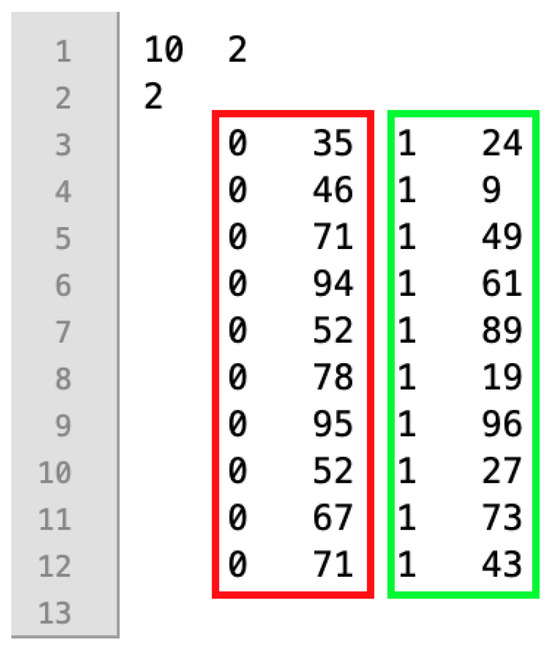
Figure 1.
Example of a problem instance of the small dataset: I_2_10_2_1.txt.
An optimal solution for this problem instance achieving a makespan of 345 is shown in Figure 2. The permutation of jobs for the machines of factory 0 is j0, j3, j8, j7, and j5, and the permutation of jobs for the machines of factory 1 is j4, j6, j2, j9, and j1. Note that the order of visiting machines for each job in both factories is first machine 0 and then machine 1 (i.e., flow-shop constraint).
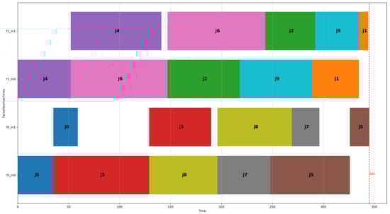
Figure 2.
The optimal solution for the first problem instance for two factories, 10 jobs, and two machines (I_2_10_2_1.txt), having an optimal makespan of 345 time units.
3. Related Work
Scheduling is such a studied area that it is considered a discipline of its own. The textbook of Pinedo [5] that is regularly updated (currently in its sixth edition) is a valuable source of information for the subject. One of the earliest contributions to machine scheduling theory and applications was Johnson’s influential work in [6]. The FSP is one of the most studied scheduling problems, as indicated by the many FSP reviews such as [7,8]. This can be attributed to the fact that having jobs that should visit machines in a predefined order is a common real-world scenario in manufacturing. The PFSP, as a more constrained version of FSP that captures well the existence of conveyor belts, has also attracted much interest [9,10]. The gap between theory and practice that was earlier identified [11] led to several extensions of the FSP and one of them is DPFSP, which is the problem investigated in this paper. Following the paper introducing the problem [1], several other papers presented new ideas and improved upon existing results [12,13]. The recent DPFSP review paper [14] highlights that DPFSP is one of the fastest-growing topics in scheduling and that several variants of the problem have emerged, besides (i.e., classic DPFSP), such as DPFSP with extra constraints (e.g., blocking/buffer, no wait, no idle, and setup times), multi-objective DPFSP, non-deterministic DPFSP, and heterogeneous DPFSP (i.e., non-identical factories). Another recent review paper that studies distributed shop scheduling both in general and concerning DPFSP in particular can be found at [15].
Many alternatives have been proposed regarding the solution approaches to the classic DPFSP. In [1], six Mixed Integer Linear Programming (MILP) formulations were proposed, alongside two factory assignment rules and 14 heuristics based on dispatching rules. The MILP formulations were unable to operate effectively due to the resulting big sizes of the models. Still, a combination of constructive heuristics with Variable Neighborhood Descent methods resulted in good solutions. In [12], Naderi et al. improved the solutions by employing a scatter search algorithm. At the same time, comparisons were made with other competitive optimization methods including a Discrete Electromagnetic metaheuristic [16], a Hybrid Genetic algorithm [17], a Variable Neighborhood Descend with Branch and Bound algorithm [18], a Tabu Search algorithm [19], an Iterated Greedy algorithm [20], and others. In [13], Ruiz et al. presented improved results, which are indeed the best known, by using Iterated Greedy algorithms employing initialization, construction, and destruction procedures, alongside local search. Comparisons were made against other approaches that also managed to produce very good results, such as a Hybrid Immune algorithm [21], a Bounded Search Iterated Greedy algorithm [22], and the Scatter Search algorithm of [12]. The recent work by Hamzadayı [23] has similarities with the approach in this paper since it employs an exact algorithm in order to address the DPFSP. In particular, it uses Benders decomposition and manages to optimally solve several problems but, as the results suggest, without satisfying the same permutation of the jobs’ constraint for all machines of the same factory. In [24], the total tardiness objective is examined, instead of the makespan using a mixed-integer linear programming model, heuristics, and two customized metaheuristics algorithms (i.e., a discrete Harris hawks optimization algorithm and a hybrid iterated greedy algorithm). Another relevant work is [25] that also employs DPFSP and attempts an optimization of the sum of three distinct objectives using exact methods and metaheuristics.
In addition to DPFSP and its lineage, many more scheduling problems exist. Some of them are inspired by specific real-world problems, while others are abstractions of original problems that are easier to study and reason about. Examples of problems belonging to the first case are the problem of scheduling independent tasks to heterogeneous multiprocessors [26] and the machine reassignment problem [27]. On the other hand, an example of the second case is the one-machine scheduling problem [28] that is an abstraction of a real-world scheduling problem that is aimed at achieving efficient charging of electrical vehicles. Another paper that proposes an approximation approach for the one-machine problem, this time including release and delivery times for the jobs, is [29].
4. Materials and Methods
The approach taken to address the DPFSP is based on modeling the problem using Constraint Programming and its specialized features for scheduling, like the interval variables and the non-overlap constraints. Then, a state-of-the-art open-source CP solver (i.e., Google’s ORTools CP-SAT [30]) is employed to solve problem instances of various sizes to assess the approach’s ability to produce competitive results. The process is accelerated when good initial solutions are fed to the solver since the solver does not spend time constructing a good solution from scratch. The good initial solutions are constructed using a known heuristic (i.e., NEH2), so the following section briefly references the vast landscape of heuristics for DPFSP and its parent problem PFSP.
4.1. Heuristics
There are several heuristics for finding solutions to the DPFSP problem, which are adaptations of heuristics for the PFSP that consider the existence of multiple factories in DPFSP. Some PFSP heuristics are shortest processing time (SPT); largest processing time (LPT); Johnson’s rule; CDS heuristic of Campbell, Dudek, and Smith; minimum idle time (MINIT); minimum completion time (MICOT); and NEH heuristic of Nawaz, Enscore, and Ham. Details about these and many more heuristics can be consulted in [31]. An interesting remark is that NEH [32] is regarded as the best-performing heuristic for PFSP when the optimization criterion is the makespan. NEH iteratively constructs a schedule by inserting jobs into an initially empty sequence. It starts by sorting the jobs in descending order based on the sum of their processing times on all machines. Then, it iteratively inserts each job into the current sequence at all possible positions and evaluates the makespan after each insertion. The job permutation that results in the shortest makespan for the partial schedule is chosen and this process is repeated until all jobs are scheduled. The worst case complexity of a naive implementation of NEH is , where n is the number of jobs and m is the number of machines, but by applying the accelerations proposed in [33], the complexity becomes .
Since DPFSP has to decide about two things: the allocation of jobs to factories and the sequence of jobs that will be processed at each factory, NEH might be combined with a rule for the allocation. Such a rule might be “assign job j to the factory which completes it at the earliest time” as proposed in [1], which gives the heuristic named NEH2, which seems to perform better than other alternatives for DPFSP. An extension of NEH2 is NEH2_en [13], which, after inserting a job into the best position among all factories, selects at random either the previous or the following job and assesses its relocation at all possible positions of the partial solution in the same factory. The worst case complexity for both NEH2 and NEH2_en is , where F is the number of factories.
In this approach, NEH2 is used to produce initial solutions for the CP solver. In particular, for each problem instance, NEH2 is executed multiple times (10 to 50, based on the size of the problem) and the best solution (i.e., the solution with the lowest makespan) is kept among all runs. Since NEH2 is deterministic, a minor modification is applied for the algorithm to return a different solution at each run. After the first run, the sequence of jobs created using the algorithm, based on the sum of each job’s processing times on all machines, is “lightly” shuffled. This occurs by taking all triplets of consecutive jobs in the original sequence and shuffling each triplet. Then, the subsequent steps of NEH2 are executed as usual. This “trick” seems to work nicely since it consistently produces better than the initial NEH2 solution for most cases, while the time burden imposed is minimal.
4.2. Model
In this section, the model of the problem is rigorously presented using a Constraint Programming point of view. Let be the set of jobs, be the set of factories, and be a set of machines. Note that each factory has an identical set of machines . Let be optional interval variables defined over all combinations of . Each optional interval variable is defined by its start time, size, and optionality. The size is a parameter integer value , denoting the processing time needed for job j at machine i, which is known in advance. Since the machines in each factory are identical, the index f does not appear at parameters . An important point is that for each job j and factory f, the interval variables for the machines of the factory share the same optional indicator, meaning that either all these interval variables are present in the solution or all of them are not present. Another set of auxiliary decision variables are boolean variables for every pair of different jobs and factory . The role of these variables is to define the order of appearance of jobs in the schedule. So, assumes value 1 when job starts before job at factory f and assumes value 0 for all other cases (i.e., when starts before at factory f, or when jobs are scheduled at different factories).
In DPFSP, each job passes through all machines of the factory that it is scheduled to, occupying the machines in the same order (permutation) as all other jobs. Hereafter, a “task” will be each process of a job at a machine. Therefore, each job comprises a sequence of tasks, with each task executed to a machine (i.e., the first task in the sequence is executed at the first machine of a factory, the second task in the sequence is executed at the second machine of the same factory, etc., as dictated by the workflow).
The objective is simply the finish time of the latest job and it should be minimized. Since each job is a sequence of tasks for the objective, examining the end times of the last tasks of all jobs as shown in Equation (1) suffices.
Next, the constraints of the problem are defined. Some constraints focus on tasks executed on machine 0 (i.e., the first machine in the series of machines that undertake the workflow) of the jobs. These constraints define how the jobs are distributed to factories and the permutation of jobs that the machines of each factory will follow. This is modeled with Equations (2) and (3). Equation (2) defines that the task of each job executed at machine 0 should be scheduled without overlaps with other tasks also executed at machine 0 of the same factory. Note that Equation (2) also determines the permutation of jobs that the machines of each factory will process. Equation (3) ensures that each job will be scheduled at exactly one factory. The equation is applied only to the first machines of each factory since, as stated earlier, all optional interval variables x for each job, factory, and factory’s machines are either all present in the solution or all of them are absent from it.
Equation (4) sets the order of appearance of jobs at each factory by enforcing order between jobs for all possible pairs of jobs. It examines the presence of x variables at the first machines of factories and whether the end time of a job is no later than the start time of another job, setting the corresponding b variable to 1.
Equation (5) ensures that binary variables b involving job j and factory f assume value 0 if job j is not scheduled to factory f. This occurs because if job j is not present in factory f, the left parts of the inequalities in Equation (5) will be 0, pushing both b variables of the right parts to 0 values. On the other hand, if job j is present in factory f, the left part of the inequalities will be two, making the constraint redundant because the sum of two binary variables will always be less or equal to two.
Equation (6) ensures that each task should start after its predecessor in the sequence of a job’s tasks. Note that the sequence of tasks for a job are executed in turn on the machines of a factory. So, this constraint ensures that the job should occupy a machine only after the job has finished processing in the preceding machines.
Equation (7) maintains the permutation of jobs set by Equation (2) for machine 0 and all other machines of the same factory. So, for every pair of jobs that are executed at the same factory f, job will either precede or follow job and this will be in accordance with the value of variable . Moreover, Equation (7) ensures that all jobs executed at machines other than machine 0 will not overlap. This occurs because given that two jobs are executed at the same factory, either variable or variable will be 1, which means that no overlap is possible because one job will start after the other job finishes.
Finally, Equation (8) is a simple symmetry breaking trick that enforces scheduling job 0 at factory 0. This occurs by setting the optional interval variable to be present at the solution, which does not exclude the optimal solution, since the factories are identical and therefore interchangeable.
The full model about the DPFSP follows:
subject to:
4.3. New Model after Throwing the Same Permutation Assumption
As stated in the introduction, adding P, which stands for permutation, to the flow-shop scheduling problem shrinks the domain space from to . This should make the work of tentative solvers easier. In this section, a Constraint Programming model is presented that throws the same permutation of jobs for all machines of each factory assumption, which results in a smaller model capable of finding better or equal solutions with respect to the solutions that the model of Section 4.2 generates.
The objective function of the model in Equation (9) remains the same as in the previous model (i.e., Equation (1)) and represents makespan. Equation (10) states that no overlapping jobs should exist for all machines of all factories. Equation (11) is identical to Equation (3) of the previous model and ensures that each job will be scheduled to exactly one factory. Equation (12) ensures that each job will be processed by the machines of the factory that undertake the execution of the job, as dictated by the sequence of machines of the factory. Finally, Equation (13) serves the same symmetry breaking goal that was described earlier in Equation (8). The full model of the new problem, which will be referred to as DFSP (Distributed Flow-shop Scheduling Problem), follows:
subject to:
The DFSP model is considerably smaller than the previous one since the b variables of the previous model are now eliminated, and, instead of six types of constraints, there are only three. Table 1 shows formulas that compute the number of decision variables and the numbers of the no_overlap and other constraints that the two models use.

Table 1.
Formulas for the number of decision variables and constraints of the DPFSP model and the DFSP model (n = numbers of jobs, m = number of machines, and F = number of factories).
Table 2 shows the numbers of constraints and the number of interval and boolean decision variables that the two models produce for some representative problem instances (i.e., the first 70 out of the 120 problem instances for the two factories and seven factories of the large dataset) of the benchmark. The great number of decision variables and constraints for problem instances after the 30th place, especially for the DPFSP model, suggest that the CP solver will probably not be able to reach optimal or near optimal solutions. Indeed, as it will be demonstrated in Section 5, the CP solver can reach optimal solutions for many problem instances of the first 30 for each group of problem instances as identified by the number of factories. But, for the subsequent 30 problem instances, the performance of the CP approach degrades and solutions are relatively far from the best-known ones. For the rest of the problem instances (i.e., places 61 to 120), the model is so big that the CP solver has trouble creating the model in the first place, let alone reaching good solutions.
Table 2.
Number of decision variables and constraints for DPFSP model and DFSP model for selected problem instances of the large dataset (rows for factories and jobs are not shown).
Figure 3 and Figure 4 show the optimal schedules that result from the DPFSP model and the DFSP model, respectively, for the fourth problem instance of the group of problems with two factories, six jobs, and four machines of the small dataset. The Y-axis of the figure displays the factories, and for each factory, each machine using the notation f<factory_id>_m<machine_id>. The schedule produced by the DFSP model has a makespan of 436 time units, which is smaller than the schedule created using the DPFSP model, which is 440 time units. The more favorable result of the schedule by the DFSP model is attributed to the fact that each machine can have a different permutation of jobs processed in it. So, in Figure 4 at factory 1, machines 0 and 1 process jobs in the sequence j4, j1, j0, j2, but machines 2 and 3 process jobs using the sequence j1, j4, j0, j2. On the other hand, as shown in Figure 3, all four machines of factory 1 peruse the same permutation of jobs, which is j4, j0, j3, j1. The greater degree of freedom given to the DFSP model allows the CP solver to find a better solution than the DPFSP for this problem instance. In Section 5, it will be seen that this occurs in many other problem instances of the small dataset and the large dataset.

Figure 3.
Optimal schedule (makespan = 440) according to the DPFSP model for the fourth problem instance with two factories, six jobs, and five machines (per factory) of the small dataset (problem instance: I_2_6_5_4).
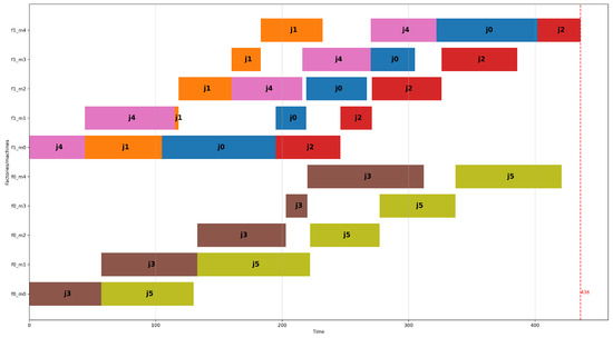
Figure 4.
Optimal schedule (makespan = 436) according to the DFSP model for the same problem instance as in Figure 3.
If the “permutation” component of the problem is added to it not as a physical requirement (e.g., conveyor belt) but as a means of making the problem easier for various solvers to search for near-optimal solutions, then dropping it does not change the gist of the problem. The DPFSP model is able to find solutions in the larger search space that allows different job permutations for the machines of the same factory, but it satisfies the vital constraint of processing each job using the same sequence of machines (i.e., workflow), which is in this case, and can be any sequence of machines by naming the machines appropriately. The “good” behavior of the DFSP model can be attributed to the efficient implementations of the global constraint no_overlap and the interval variables that the CP solver employs.
4.4. A Novel Heuristic for Achieving Lower Bounds
This section presents a heuristic for computing lower bounds of problem instances that apply to DPFSP and DFSP. Let be the index of the machine in a series of machines that is replicated across all factories. The heuristic evenly distributes the total process time of all jobs at machine i of a factory. This should ideally occur when the total process time of all jobs at machine i is divided by the number of factories, giving value . The lower bound is computed by examining each machine i in the series of machines in turn. For each machine i, two values are computed: the shortest total execution time of a job for machines that precede machine i, and the shortest total execution time of a job for the machines that come after machine i. Potential lower bounds are calculated by adding these two minimum values to . Finally, the maximum of the potential lower bounds for all machines is the lower bound. Algorithm 1 describes the procedure in pseudo-code.
| Algorithm 1 Lower Bound Heuristic |
|
The main idea behind the computation of the lower bound is depicted in Figure 5, where at the left of the figure, the situation is shown where machine i is the first machine; in the right of the figure, the situation of machine i is the last machine is depicted; and in the middle of the figure, the situation is depicted where the machine i is any machine in between.

Figure 5.
Makespan lower bounds considering execution of all jobs without gaps at each machine in turn.
A proof of the validity of the lower bound follows:
Proof of the Validity of the Lower Bound.
For computing the lower bound we assume that at a certain machine i, all jobs are scheduled without any gaps between them. This naturally occurs at machine 0, but it can also occur at other machines too. Note that gaps might occur for each machine because the start of a job at this machine must be postponed until the same job finishes at machine and the job that was previously processed at machine i has finished its execution. Let be the average process time of all jobs at machine i ( is computed by totaling the process times of all jobs at machine i and dividing it by the number of factories). Then, let be the minimum sum of process times for machines that precedes machine i, among all jobs, by a single job. Likewise, let be the minimum sum of process times for machines that come after machine i, among all jobs, by a single job. Clearly, when machine i is the first machine, will be zero, and when machine i is the final machine, will be zero. We assert that the maximum among all machines will be a lower bound for the problem.
Let us assume that we know the optimal solution, where for each machine, the jobs are scheduled as dictated by a specific permutation of jobs, with possible gaps in between consecutive jobs. Let be the duration from the time that machine i starts processing to the time that it finishes processing the last job in the optimal solution, at a factory where . We are sure that such a factory exists because the average value of a set is always less or equal than its maximum value. Moreover, let be the time that machine i starts processing. This time is shifted to the right due to the process of the first job in the optimal solution at the machines that precede machine i. Likewise, let be the duration between finishing processing for the last job of the optimal permutation at machine i and the makespan of the schedule. It holds that because by definition, is the smallest possible total process duration among all jobs. Likewise, , since is again the smallest possible total process duration of a single job among all jobs for machines after machine i. So, it follows that . Based on this observation, we expect the maximum among for all machines i to be a lower bound for the problem. □
5. Results
The experiments that gave the results reported in this section were all obtained via runs on an Apple Mac mini, with an M2 Pro chip having 10 cores (six performance and four efficiency) and 16 GB of RAM. The solver used was Google’s ORTools (version 9.7.2996) [30] and its CP-SAT solver. All of the code was written in plain Python (version 3.10).
5.1. Lower Bounds Derived via the Heuristic
Here, the results generated by the lower bound heuristic described in Section 4.4 are presented. Figure 6 and Figure 7 show the percentage difference of the lower bounds that the heuristic produces with respect to the best-known values for all problem instances of the benchmark’s small dataset and large dataset, respectively. The problem instances for the small and large datasets are grouped based on the number of factories. For each group for the small dataset, the problem instances are arranged in a sequence where the number of jobs is 4, 6, 8, 10, 12, 14, and 16, and the number of machines is two, three, four, and five, while the five problem instances exist for each combination of the number of jobs and the number of machines. Likewise, for each group of problem instances of the large dataset, the sequence of problem instances contains 10 problem instances for each combination of jobs and machines as described in Section 2.1.

Figure 6.
Distance of lower bounds to the best-known values for problem instances of the “small” dataset. Order of appearance of problem instances in x-axis: .
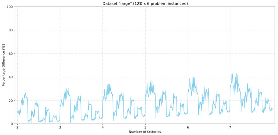
Figure 7.
Distance of lower bounds to the best-known values for problem instances of the “large” dataset.
By examining lower bound values for the problem instances of the small dataset, one case (i.e., I_2_16_2_5) was identified where the lower bound computed via the heuristic is equal to the optimal solution of the problem.
By observing the two figures, it can be seen that there is a tendency to increase the percentage difference when the number of factories increases. Moreover, for each dataset (i.e., small and large) for problem instances with the same number of factories, the percentage differences tend to decrease for problem instances with greater numbers of jobs and machines.
The values of the lower bounds produced by the heuristic for all problem instances can be consulted at the GitHub repository https://github.com/chgogos/DPFSP_CP, accessed on 2 November 2023.
5.2. Results for Problem Instances of the Small Dataset
The DPFSP model’s results for all 420 instances of the small dataset are excellent. All problem instances are solved to optimality, where the optimality is reached for each instance in a matter of seconds or less. The maximum time needed for solving an instance was 1.44 s (for instance, I_3_16_5_3), while the average time of solving them was 0.14 s per instance (i.e., 58.8 s to solve all instances of the small dataset optimally).
Applying the DFSP model, the makespans of many problem instances are further minimized, since now the model constraints allow for such solutions to exist. Indeed, there are 65 problem instances having solutions with smaller makespans than the makespans of the optimal solutions for the DPFSP model and these problem instances, alongside their solutions, are presented in Table A1 in Appendix A. The last column of the table shows the job permutations assigned to each factory machine in the format of a string where the factories are separated with semicolons and the machines of each factory are separated with commas. For each machine, the sequence of jobs is indicated as a string of job ids separated by dashes. So, for example, in the first line of the table, for problem instance I_2_6_5_4, the solution “3-5,3-5,3-5,3-5,3-5;4-1-0-2,4-1-0-2,1-4-0-2,1-4-0-2,1-4-0-2” at the rightmost column means that factory 0 processes the sequence of jobs 3-5 in all of its five machines and factory 1 processes the sequence of jobs 4-1-0-2 for machines 0, 1, and 2, but the sequence changes for machines 3 and 4 to 1-4-0-2. This allows for us to achieve a better makespan value of 436 over 440, (as already seen in Figure 3 and Figure 4), which would have been the optimal solution if the permutation of jobs remained the same for all machines of factory 1, as is dictated by the DPFSP problem statement. Again, the solutions reached for all problem instances are the optimal ones according to the DFSP model and all solutions are reached almost immediately (i.e., maximum time = 3.54 s, for instance I_2_16_4_1, average time = 0.087 s, and total time needed to optimally solve all instances = 36.12 s).
The complete list of objective costs, execution times, and permutations of jobs that are given to the machines of each factory for all problem instances of the small dataset, for the DPFSP model and for the DPSP model, can be found at https://github.com/chgogos/DPFSP_CP, accessed on 2 November 2023.
5.3. Results for Problem Instances of the Large Dataset
Experiments were also run for problem instances of the large dataset. The problem instances selected were the smaller ones of the large dataset. Experiments only used the first 30 problem instances for each case of two, three, four, five, six, and seven factories, totaling 180 problem instances. This means there were 10 problem instances for each case of scheduling 20 jobs at 5, 10, and 20 machines per factory for two to seven factories. Other problem instances that involved 50, 100, 200, and even 500 jobs, starting at problem index 31 for each factory number group, proved to be beyond the capabilities of this paper’s approach for producing optimal results. This behavior was anticipated since the size of the problem (i.e., number of decision variables, number of constraints) assumes high values starting at problem index 31 (i.e., jobs = 50) and reaches extremely high values for problem instances with 100, 200, and 500 jobs.
This paper’s approach optimally solved the majority of the problem instances within the time allotted for execution to the CP solver, which was 300 s on the hardware and software setting described at the beginning of Section 5. In particular, optimal values were found for 13 out of the 30 problem instances for two factories and for all problem instances ( problem instances) for three, four, five, six, and seven factories. Moreover, comparison with the best-known results of Ruiz et al. [13] revealed that all best-known results were reached, proving that 163 of them are indeed optimal. For the 17 problem instances that the CP approach proposed in this paper was not able to prove optimality within the allotted time, a lower bound is provided by the approach instead. These lower bounds (all about problem instances with two factories) are presented in the Appendix A at Table A2. Furthermore, the solutions’ objective (i.e., makespan), the best-known objective values, and the time needed, either due to the 300 s timeout or because the optimal solution was found, are presented in Appendix A at Table A2, Table A3, Table A4, Table A5, Table A6 and Table A7. In the column “Makespan” of these tables, the star symbol indicates an optimal result, while the plus symbol indicates that the solution is not proven optimal but is equal to the best-known solution.
The time needed to prove optimality for each problem instance that is eventually proved optimal is usually longer than the time needed to reach the optimal value. Indeed, by analyzing these times, it was found that, on average, the optimal value is reached at a fraction of the time needed to prove optimality. This is graphically shown in Figure 8. Moreover, Table 3 shows statistics across the problem instances about how many times reaching optimality is faster than proving optimality.
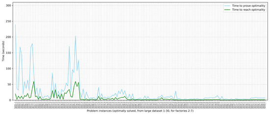
Figure 8.
Time needed by the exact solver to prove optimality vs. time needed to reach the optimal solution for 163 problem instances where the optimal solution is reached within 300 s.
Table 3.
Statistics about how many times reaching an optimal solution is faster than proving it is indeed optimal.
The DFSP model has also been applied to the same problem instances (i.e., the first 30 instances for factories in 2,3,4,5,6,7) of the large dataset. Among the solutions for the 180 problem instances, 133 were optimally solved within 300 s of execution time. The comparison of the solutions with the best-known solutions for the DPFSP model showed that, on 142 of them, the solution that the DFSP model produced is better. On 33 problem instances, the solutions of the DFSP model are equal to the best-known solutions for the DPFSP model, and in only five problem instances, the solutions’ objective values are worse (Ta_013_2 with 1008 instead of 1001, Ta_018_2 with 1027 instead of 1025, Ta_021_2 with 1676 instead of 1674, Ta_027_2 with 1677 instead of 1671, and Ta_028_2 with 1621 instead of 1610). Figure 9 compares the execution times that were needed by the solver to reach optimality for both the DPFSP and DFSP models, for problem instances that were optimally solved within 300 s. As expected, the DFSP model, having more degrees of freedom, is a more difficult problem, and for the majority of problem instances, it needs more time to prove optimality. Nevertheless, this effect is minimized when more factories are added. This can be attributed to the fact that the number of jobs that are distributed to each factory becomes smaller when more factories exist, resulting in fewer possible schedules per factory.
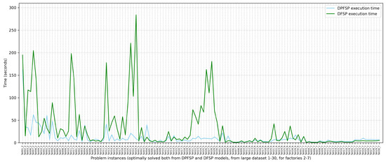
Figure 9.
Time needed by the exact solver to prove optimality for the DPFSP model vs. the DFSP model, for 133 problem instances where optimality is reached by both models within 300 s.
The complete list of objective costs, execution times, and permutations of jobs that are given to the machines of each factory for all problem instances of the large dataset, for the DPFSP model and the DPSP model, can be found at https://github.com/chgogos/DPFSP_CP, accessed on 2 November 2023.
6. Discussion
In optimization, exact methods backed up by solvers like CP solvers, MIP solvers, SAT solvers, and others have several advantages over approximate methods like heuristics, meta-heuristics, and hyper-heuristics. They provide global optimality with theoretical guarantees, they compute lower bounds, and, during execution, they provide information about the gap between the current solution and the current lower bound. Nevertheless, they have disadvantages like the difficulty in modeling complex real-world situations, the long execution times, and, of course, the combinatorial explosion problem that refers to the rapid growth in the number of possible solutions when dealing with combinatorial problems (i.e., problems of making selections, arrangements, or choices from a finite set of discrete elements or objects, often subject to certain constraints or conditions). The DPFSP is such a problem that the number of decision variables and constraints quickly become astronomically large.
In the experiments, the execution time allowed for each problem instance was only 300 s. Experiments using 300 s of execution time for the problem instances with 50 jobs returned mediocre results. It is expected that better results will be found, more solutions will be verified as optimal, and perhaps new optimal solutions will be identified once more execution time is given. This might be advantageous for problem instances with 50 jobs, where a few hours of execution time for each problem instance should reveal good results, as some preliminary experiments have indicated. Nevertheless, this does not scale for problem instances with even more jobs (e.g., 100 jobs or more).
The CP approach can be used in DPFSPs of very large sizes, provided that a solution is built and that the CP solver “sees” only a manageable size of the otherwise intractable via the CP model’s full problem. In such scenarios, the selection of jobs, factories, and machines that might be free to be moved by the CP solver can be decided randomly or based on a pattern (e.g., allow for task rearrangement in a single factory, allow for the move of a small number of tasks of relatively big sizes together with tasks of smaller sizes, and allow for the move of tasks that are responsible for the current makespan).
Another idea for further improving the results or addressing larger problem sizes is to use the solution that the less heavy DFSP model produces and then try to repair it to satisfy the DPFSP problem’s permutation constraint. Indeed, the attempt of repair might be undertaken by the DPFSP model, allowing it to move only a subset of the problem’s tasks.
When the modified NEH heuristic provided relatively good solutions, a strange behavior was noticed for problem instances of big sizes (e.g., jobs = 50 or bigger). The CP solver used (Google’s ORTools) greatly delayed creating the starting solution, and in some cases, the 300 s were not enough to return a solution. This might be caused by the setup of the internal data structures that the CP solver uses in order to continue the search process. Of course, more CP solvers can be used, including the IBM ILOG CP solver and others.
Another remark worth noticing is that for the problem instances of the large dataset with 20 jobs, it proved easier to find optimal solutions when many factories existed (e.g., seven), rather than when there were only two factories. This can be explained by noticing that once the jobs are distributed in the many factories, the combinations of jobs that can be arranged in each factory are significantly smaller.
Finally, a few remarks can be made about the proposed heuristic in Section 5.1 that finds lower bounds. Firstly, it is expected that once the problem increases in size, the lower bounds derived by heuristics will be less tight, and this is indeed the case. Secondly, the usefulness of lower bounds should be highlighted since they can help in assessing the effectiveness of solutions that have no other way of knowing how good they are. Finally, values computed by the heuristic are lower bounds for the DPFSP and DFSP problems.
7. Conclusions
The Distributed Permutation Flow-shop Scheduling Problem (DPFSP) is a problem that originated from the famous Permutation Flow-shop Scheduling problem relatively recently and managed to attract the attention of many researchers. This can be attributed to the fact that nowadays, the modern manufacturing world is more distributed than ever, with many factories processing together deliveries that must be completed in an optimal manner.
This work presented an approach to the problem based on formulating it using Constraint Programming (CP) and its scheduling features (i.e., interval variables and non-overlap constraints). Two models were presented: one for the original problem (i.e., DPFSP) and one for the problem after dropping the same permutation of jobs across all machines of each factory constraint. Both models were simple enough and managed to solve optimal problem instances of sizes that were, to the best of my knowledge, previously unable to be solved using an exact method. Moreover, a novel way of computing lower bounds for DPFSP was presented that was capable of generating relatively tight lower bounds. The approaches were tested on known public datasets for the DPFSP and the results suggest that CP is a viable choice for the problem, given the advances that the theory has made in this area, the capable implementation of CP solvers, and the processing capabilities of modern commodity computer systems.
Funding
This research received no external funding.
Institutional Review Board Statement
Not applicable.
Informed Consent Statement
Not applicable.
Data Availability Statement
Results of this research can be found at the github repository https://github.com/chgogos/DPFSP_CP, accessed on 2 November 2023. The dataset that was used for the Distributed Permutation Flow-shop Scheduling Problem are public and were made available by the research group “Sistemas de Optimización Aplicada SOA”. A mirror of the dataset is kept in https://github.com/chgogos/DPFSP_CP/blob/main/DPFSP.7z, accessed on 2 November 2023.
Conflicts of Interest
The author declares no conflict of interest.
Abbreviations
The following abbreviations are used in this manuscript:
| CP | Constraint Programming |
| DFSP | Distributed Flow-shop Scheduling Problem |
| DPFSP | Distributed Permutation Flow-shop Scheduling Problem |
| FSP | Flow-shop Scheduling Problem |
| JSP | Job-shop Scheduling Problem |
| NHE | Nawaz, Enscore, and Ham heuristic |
| PFSP | Permutation Flow-shop Scheduling Problem |
| SAT | Satisfiability |
Appendix A
Table A1.
65 of the 420 problem instances of the small dataset that have as optimal makespan a smaller value for the DFSP model than the optimal makespan for the DPFSP model.
Table A1.
65 of the 420 problem instances of the small dataset that have as optimal makespan a smaller value for the DFSP model than the optimal makespan for the DPFSP model.
| Instance | DPFSP Makespan | DFSP Makespan | Time (s) | Jobs Permutation per Machine per Factory |
|---|---|---|---|---|
| I_2_6_5_4 | 440 | 436 | 0.01 | 3-5,3-5,3-5,3-5,3-5;4-1-0-2,4-1-0-2,1-4-0-2,1-4-0-2,1-4-0-2 |
| I_2_8_5_1 | 468 | 457 | 0.01 | 2-5,2-5,5-2,5-2,5-2;0-1-4-6-7-3,0-1-4-6-7-3,0-1-4-6-7-3,0-1-4-6-7-3,0-1-4-6-7-3 |
| I_2_8_5_4 | 463 | 459 | 0.02 | 2-7-1-3,2-7-1-3,2-1-7-3,2-1-7-3,2-1-7-3;4-0-6-5,4-0-6-5,0-4-6-5,0-4-6-5,0-4-6-5 |
| I_2_8_5_5 | 376 | 372 | 0.02 | 5-2-7,5-2-7,5-2-7,5-2-7,5-2-7;6-0-4-3-1,6-0-4-3-1,6-4-0-3-1,6-4-0-3-1,6-4-0-3-1 |
| I_2_10_4_2 | 415 | 414 | 0.02 | 0-2-8-5-1,0-2-8-5-1,0-2-8-5-1,0-2-8-5-1;3-4-9-7-6,3-4-9-7-6,3-4-9-6-7,3-4-9-6-7 |
| I_2_10_5_2 | 439 | 432 | 0.03 | 8-9-7-5,8-9-7-5,9-8-7-5,9-8-7-5,9-8-7-5;2-3-4-1-0-6,2-3-4-1-0-6,2-3-4-1-0-6,2-3-4-1-0-6,2-3-1-4-0-6 |
| I_2_10_5_3 | 518 | 512 | 0.04 | 4-5-2-6,4-5-2-6,4-5-2-6,4-5-2-6,4-5-2-6;8-3-9-1-0-7,8-3-9-1-0-7,3-8-9-1-0-7,3-8-9-1-0-7,3-8-9-1-0-7 |
| I_2_12_4_2 | 460 | 455 | 0.05 | 2-6-10-4-3-1,2-6-10-4-3-1,2-6-10-4-3-1,2-6-10-4-3-1;8-9-11-7-0-5,8-9-11-7-0-5,8-9-11-7-5-0,9-8-11-7-5-0 |
| I_2_12_4_5 | 410 | 405 | 0.04 | 4-1-9-3-0,4-1-9-3-0,4-1-9-0-3,4-1-9-0-3;11-8-6-7-5-2-10,11-8-6-7-5-2-10,11-8-7-6-5-2-10,11-8-7-6-5-2-10 |
| I_2_12_5_2 | 443 | 440 | 0.15 | 5-6-10-8-7-3-0,6-5-10-8-7-0-3,6-5-10-8-7-0-3,6-5-8-10-7-0-3,6-5-8-10-7-3-0;1-2-11-4-9,1-2-11-9-4,1-2-11-9-4,1-11-2-9-4,1-11-2-9-4 |
| I_2_12_5_3 | 488 | 485 | 0.06 | 8-10-11-6-4,8-10-11-6-4,8-10-11-6-4,8-10-11-6-4,8-10-11-6-4;1-7-2-9-3-5-0,1-7-2-9-3-5-0,1-7-2-3-9-5-0,1-7-2-3-9-5-0,1-7-2-3-5-9-0 |
| I_2_12_5_4 | 492 | 487 | 0.08 | 0-10-9-4-7-5,0-10-9-4-5-7,0-10-9-4-5-7,0-10-9-5-4-7,0-10-9-5-7-4;3-11-6-8-2-1,3-11-6-8-2-1,3-11-6-8-2-1,3-11-6-8-2-1,3-11-6-8-2-1 |
| I_2_12_5_5 | 573 | 572 | 0.11 | 6-4-10-5-1-0,6-4-10-5-1-0,6-4-10-5-1-0,6-10-4-5-1-0,6-10-4-1-5-0;7-9-3-8-2-11,7-9-3-8-2-11,7-9-3-8-2-11,7-9-3-8-2-11,7-9-3-8-2-11 |
| I_2_14_4_1 | 458 | 457 | 0.11 | 12-4-11-9-5,12-4-11-9-5,12-4-11-9-5,12-4-11-9-5;10-13-6-0-1-8-3-7-2,10-6-0-13-1-8-3-7-2,10-6-0-1-13-8-3-7-2,10-6-0-1-8-3-7-2-13 |
| I_2_14_5_1 | 536 | 534 | 0.2 | 8-10-7-12-0-6-2,8-10-7-12-0-6-2,8-10-7-12-0-6-2,8-10-7-12-0-6-2,8-10-7-12-0-6-2;9-4-13-5-3-1-11,9-4-13-5-3-1-11,9-4-13-3-5-1-11,9-4-13-3-5-1-11,9-4-13-3-5-1-11 |
| I_2_14_5_2 | 553 | 551 | 0.14 | 11-9-12-8-3-5-7,11-9-12-8-3-5-7,11-9-12-8-3-5-7,11-9-12-3-8-5-7,11-9-12-3-8-5-7;4-10-6-0-13-1-2,4-10-0-13-6-1-2,4-10-0-13-6-1-2,4-10-0-13-6-1-2,4-10-0-13-6-1-2 |
| I_2_14_5_3 | 558 | 555 | 0.22 | 4-3-13-2-0-11,4-3-13-2-0-11,4-3-13-2-11-0,4-3-13-2-11-0,4-3-13-2-11-0;5-1-7-9-6-10-12-8,5-1-7-9-6-10-12-8,5-1-7-9-10-6-12-8,5-1-7-9-10-12-6-8,5-1-7-9-10-12-6-8 |
| I_2_14_5_4 | 480 | 474 | 0.37 | 6-4-12-7-3-9-10-1,6-4-12-7-9-10-3-1,6-4-12-7-9-10-3-1,6-4-12-7-9-10-3-1,6-4-12-7-9-10-3-1;13-2-8-0-11-5,13-2-8-0-11-5,13-2-8-11-0-5,2-13-8-11-0-5,2-13-8-0-11-5 |
| I_2_14_5_5 | 541 | 538 | 0.21 | 2-9-4-3-0-11-13,2-9-4-3-0-13-11,2-9-4-3-0-13-11,2-9-4-0-3-13-11,2-9-4-0-3-13-11;7-10-5-6-1-12-8,7-10-5-6-1-12-8,7-10-5-6-1-12-8,7-5-10-6-1-12-8,7-5-10-6-1-12-8 |
| I_2_16_4_1 | 585 | 583 | 3.54 | 13-4-7-6-5-3-8,13-4-7-6-5-3-8,13-4-7-6-5-3-8,13-4-7-6-5-3-8;0-12-14-15-2-1-11-10-9,0-14-12-15-2-1-11-10-9,14-0-12-15-2-1-11-10-9,14-12-0-15-2-1-10-11-9 |
| I_2_16_4_2 | 588 | 587 | 0.45 | 7-6-5-15-3-13-2,7-6-5-15-3-13-2,7-6-5-3-15-13-2,7-6-5-3-15-13-2;10-1-12-14-9-8-11-4-0,10-1-12-14-9-11-8-4-0,10-1-12-14-9-11-8-4-0,10-1-12-14-9-11-8-4-0 |
| I_2_16_5_1 | 526 | 523 | 1.82 | 2-9-5-6-14-12-1-0,2-9-5-6-14-12-1-0,2-9-5-6-14-12-1-0,2-9-5-6-14-12-1-0,2-9-5-6-14-12-1-0;8-13-11-7-4-3-10-15,8-13-11-7-4-3-10-15,8-13-11-7-4-3-10-15,8-13-11-4-7-3-10-15,8-13-11-4-7-3-10-15 |
| I_2_16_5_3 | 652 | 649 | 1.83 | 5-15-7-8-1-12-10,5-15-7-8-1-12-10,5-15-7-8-1-12-10,5-15-7-8-1-12-10,5-15-7-8-1-12-10;6-4-0-13-14-9-11-2-3,6-4-0-14-13-9-11-2-3,4-0-6-14-13-9-11-2-3,4-0-6-14-13-9-11-2-3,4-0-6-13-14-9-11-2-3 |
| I_2_16_5_5 | 653 | 646 | 0.83 | 14-11-0-15-7-1-13-2,14-15-0-7-11-1-13-2,14-15-0-7-1-11-13-2,14-15-0-1-7-11-13-2,14-15-0-1-7-11-13-2;12-10-6-3-4-9-8-5,12-10-6-3-4-9-8-5,12-10-6-3-4-9-8-5,12-10-3-6-4-9-8-5,12-10-3-6-4-9-8-5 |
| I_3_6_5_3 | 413 | 380 | 0.01 | 0,0,0,0,0;3-4-1,3-4-1,3-4-1,3-4-1,3-4-1;2-5,2-5,2-5,5-2,5-2 |
| I_3_6_5_4 | 388 | 382 | 0.01 | 5,5,5,5,5;4-0,4-0,4-0,4-0,4-0;2-3-1,2-3-1,2-1-3,2-1-3,2-1-3 |
| I_3_8_5_1 | 344 | 342 | 0.02 | 6,6,6,6,6;0-7-4,0-7-4,0-7-4,0-7-4,0-7-4;5-3-2-1,5-3-2-1,5-3-2-1,3-5-2-1,3-5-2-1 |
| I_3_8_5_2 | 320 | 319 | 0.02 | 2-3,2-3,2-3,3-2,3-2;0-6-4,0-6-4,0-6-4,0-6-4,0-6-4;5-1-7,5-1-7,5-1-7,1-5-7,1-5-7 |
| I_3_12_4_1 | 357 | 353 | 0.04 | 8-9-10-4,8-9-10-4,8-9-10-4,8-9-10-4;11-0-6-5,11-0-6-5,0-11-6-5,0-11-6-5;7-1-2-3,7-1-2-3,7-1-2-3,7-1-2-3 |
| I_3_12_4_4 | 414 | 408 | 0.06 | 8-10-0,8-10-0,8-10-0,8-10-0;1-2-9-3,1-2-9-3,1-2-9-3,1-2-9-3;4-11-7-5-6,4-11-7-5-6,4-11-5-7-6,4-11-5-7-6 |
| I_3_12_5_3 | 438 | 431 | 0.04 | 2-8-5,2-8-5,2-8-5,2-8-5,2-5-8;4-0-11-1-7,4-0-11-1-7,4-0-11-1-7,0-4-11-1-7,0-4-11-1-7;9-10-3-6,9-10-3-6,9-10-3-6,9-10-6-3,9-10-6-3 |
| I_3_12_5_4 | 414 | 413 | 0.04 | 8-11-6,8-11-6,8-11-6,8-6-11,8-6-11;10-4-3-0,10-4-3-0,10-4-3-0,10-4-3-0,10-3-4-0;5-1-9-7-2,5-1-9-7-2,5-1-7-2-9,5-1-7-2-9,5-1-7-2-9 |
| I_3_14_4_5 | 381 | 371 | 0.08 | 4-9-5-10,4-9-10-5,4-10-9-5,4-10-9-5;11-3-7-0-1-6,11-3-7-0-1-6,11-3-7-0-1-6,11-3-7-0-1-6;2-13-8-12,2-13-8-12,2-13-8-12,2-13-8-12 |
| I_3_14_5_2 | 497 | 491 | 0.14 | 8-12-11-1,8-12-11-1,8-12-11-1,8-12-11-1,8-12-11-1;9-6-10-3-0,9-6-10-3-0,9-6-10-3-0,9-6-3-10-0,9-6-3-10-0;13-4-7-2-5,13-4-7-2-5,13-4-7-2-5,13-4-7-2-5,13-4-7-2-5 |
| I_3_14_5_4 | 494 | 490 | 0.13 | 5-9-10-0-6,5-9-10-0-6,5-9-10-0-6,5-9-10-6-0,5-9-10-6-0;7-13-2-1,7-13-2-1,7-13-2-1,7-13-1-2,7-13-1-2;11-12-3-8-4,11-12-3-8-4,11-12-3-8-4,11-12-3-8-4,11-12-3-8-4 |
| I_3_14_5_5 | 491 | 489 | 0.44 | 10-2-1-3,10-2-1-3,10-2-1-3,10-2-1-3,10-2-1-3;9-6-5-4-0,9-6-5-4-0,9-6-5-4-0,9-6-5-4-0,9-6-5-4-0;8-7-12-11-13,8-7-12-11-13,8-12-11-7-13,8-12-11-7-13,12-8-11-7-13 |
| I_3_16_3_1 | 340 | 339 | 0.15 | 4-15-2-8,4-2-8-15,4-2-8-15;3-10-7-0-13-14,3-7-10-0-13-14,3-10-7-0-13-14;1-5-9-11-6-12,1-5-9-11-6-12,1-5-9-11-6-12 |
| I_3_16_3_3 | 350 | 349 | 0.1 | 4-12-1-10,4-12-1-10,4-12-1-10;2-11-6-15-0-13-5,2-11-6-15-0-13-5,2-11-6-15-0-13-5;3-7-14-8-9,3-7-14-8-9,3-7-14-8-9 |
| I_3_16_3_5 | 362 | 361 | 0.12 | 9-3-7-14-15,9-3-7-14-15,9-3-7-14-15;1-0-2-12-6,1-0-2-12-6,1-0-2-12-6;10-8-11-5-4-13,10-8-11-5-4-13,10-8-11-5-4-13 |
| I_3_16_4_1 | 422 | 421 | 0.32 | 1-11-9-12-8,1-11-9-12-8,1-11-9-12-8,1-11-9-12-8;10-5-7-3-0,10-5-7-3-0,10-5-7-3-0,10-5-7-3-0;2-15-4-6-14-13,2-15-4-6-14-13,15-2-4-6-13-14,15-4-2-6-13-14 |
| I_3_16_4_2 | 458 | 457 | 0.27 | 12-1-11-7-13,12-11-7-13-1,12-11-7-13-1,12-11-7-13-1;15-5-2-8-3-0,15-5-2-8-3-0,15-5-2-8-3-0,15-5-2-8-3-0;4-9-14-10-6,4-9-14-10-6,4-9-14-10-6,4-9-14-10-6 |
| I_3_16_4_3 | 421 | 417 | 0.17 | 11-7-5-6-4-14,11-7-5-6-4-14,11-7-6-5-14-4,11-7-6-5-14-4;13-12-2-0-9,13-12-2-0-9,13-12-2-0-9,13-12-2-0-9;3-10-1-15-8,3-10-1-15-8,3-10-1-15-8,3-10-1-15-8 |
| I_3_16_4_4 | 430 | 429 | 0.36 | 0-13-2-6-7,0-13-2-6-7,0-13-2-7-6,0-13-2-7-6;5-10-9-8-1-11,5-10-9-8-1-11,5-10-9-8-1-11,5-10-9-8-1-11;4-3-15-12-14,4-3-15-12-14,4-3-15-12-14,4-3-15-12-14 |
| I_3_16_4_5 | 419 | 411 | 0.33 | 12-1-10-5-4,12-1-10-5-4,1-12-10-5-4,1-12-10-5-4;6-3-8-9-14-0,6-3-8-9-14-0,6-3-8-9-14-0,6-3-8-9-14-0;11-13-2-15-7,11-13-2-15-7,11-13-2-15-7,11-13-2-15-7 |
| I_3_16_5_1 | 453 | 449 | 0.23 | 9-3-8-11-5,9-3-8-11-5,9-3-8-11-5,9-3-8-11-5,9-3-8-11-5;6-0-10-13-15-14-2,6-0-10-13-15-14-2,6-10-0-13-15-14-2,6-10-0-13-15-14-2,6-10-0-13-15-14-2;4-1-7-12,4-1-7-12,4-1-7-12,4-1-7-12,4-1-7-12 |
| I_3_16_5_2 | 500 | 499 | 2.45 | 12-15-11-4,12-15-11-4,12-15-11-4,12-15-11-4,12-15-11-4;0-2-5-13-10-14-3,0-2-5-10-13-14-3,0-2-5-10-13-14-3,0-2-5-10-13-14-3,0-5-10-2-13-14-3;9-7-6-8-1,9-7-6-8-1,9-7-6-8-1,9-7-6-8-1,9-7-6-8-1 |
| I_3_16_5_3 | 476 | 475 | 1.42 | 15-11-6-4-10,15-11-6-10-4,15-11-6-4-10,15-11-6-4-10,15-11-6-4-10;14-3-1-0-5,14-1-0-5-3,1-14-0-5-3,1-14-0-5-3,1-14-0-5-3;8-9-7-12-2-13,8-9-7-12-2-13,8-9-12-7-2-13,8-9-12-7-2-13,8-9-12-7-2-13 |
| I_3_16_5_4 | 524 | 519 | 0.6 | 10-0-14-2-11,10-0-14-2-11,10-0-14-2-11,10-0-14-2-11,0-10-14-2-11;3-8-12-1-6-7,3-8-12-1-6-7,3-8-12-1-6-7,3-8-12-1-6-7,3-8-12-1-6-7;5-9-13-15-4,5-9-13-15-4,5-9-15-13-4,5-9-15-13-4,9-5-15-13-4 |
| I_3_16_5_5 | 473 | 469 | 0.89 | 6-2-12-3-0,6-2-12-3-0,2-6-12-3-0,2-6-12-3-0,2-6-12-3-0;11-13-1-8-4,11-13-1-8-4,11-13-1-8-4,11-13-1-8-4,11-13-1-8-4;15-10-5-14-7-9,15-10-5-14-7-9,10-15-5-14-7-9,10-15-14-5-9-7,10-15-14-5-9-7 |
| I_4_12_4_1 | 290 | 286 | 0.04 | 3-5,3-5,5-3,5-3;4-11-9-1,4-11-9-1,4-11-9-1,4-11-9-1;8-2-7,8-2-7,8-2-7,8-2-7;10-6-0,10-6-0,10-6-0,10-6-0 |
| I_4_12_4_5 | 331 | 327 | 0.04 | 1-7-4,1-7-4,1-7-4,1-7-4;8-11-2,8-11-2,8-2-11,8-2-11;6-10,6-10,6-10,6-10;0-3-5-9,0-3-5-9,0-3-5-9,0-3-9-5 |
| I_4_12_5_2 | 396 | 395 | 0.05 | 5-3,5-3,5-3,5-3,5-3;1-8-9-7,1-9-8-7,1-9-8-7,1-9-8-7,1-9-7-8;6-2-4,6-2-4,6-2-4,2-6-4,2-6-4;11-0-10,11-0-10,11-10-0,11-10-0,11-10-0 |
| I_4_12_5_3 | 415 | 411 | 0.06 | 1-2-0,1-0-2,1-0-2,1-2-0,1-0-2;4-5,4-5,4-5,5-4,5-4;8-11-7,8-11-7,8-11-7,8-11-7,8-11-7;3-9-10-6,3-9-10-6,3-9-10-6,3-9-10-6,3-9-10-6 |
| I_4_12_5_4 | 372 | 360 | 0.05 | 6,6,6,6,6;8-11-1,8-11-1,8-11-1,8-1-11,8-1-11;4-10-5,4-10-5,4-10-5,4-10-5,4-10-5;7-9-0-2-3,7-9-0-2-3,7-9-0-2-3,7-9-0-3-2,7-9-0-3-2 |
| I_4_14_4_5 | 297 | 292 | 0.06 | 4-12-13,4-12-13,4-12-13,4-12-13;8-5-10,8-5-10,8-5-10,8-5-10;3-9-6-7,3-9-6-7,3-9-7-6,3-9-7-6;0-2-1-11,0-2-1-11,0-2-1-11,0-2-1-11 |
| I_4_14_5_1 | 398 | 397 | 0.14 | 8-9-5-6,8-9-5-6,8-9-5-6,8-5-9-6,8-5-9-6;3-7-11,3-7-11,3-7-11,3-7-11,3-7-11;10-13-12,10-13-12,10-13-12,13-10-12,13-10-12;0-1-2-4,0-1-2-4,0-1-2-4,0-1-2-4,0-1-2-4 |
| I_4_14_5_4 | 425 | 423 | 0.12 | 7-11,7-11,7-11,7-11,7-11;13-4-1-3,13-4-1-3,13-4-1-3,13-4-1-3,13-4-1-3;6-12-9-10,6-12-9-10,6-12-9-10,6-12-10-9,6-12-10-9;0-2-8-5,0-2-8-5,0-8-2-5,0-8-2-5,0-8-2-5 |
| I_4_14_5_5 | 432 | 427 | 0.1 | 2-9-3,2-3-9,2-3-9,2-3-9,2-3-9;4-13-1-5,4-13-1-5,4-13-1-5,4-13-1-5,4-13-1-5;11-6-12-10,11-6-12-10,11-6-12-10,11-6-12-10,11-6-12-10;7-0-8,7-0-8,7-0-8,0-7-8,0-7-8 |
| I_4_16_3_3 | 312 | 311 | 0.06 | 0-6-2-1,0-6-2-1,0-6-2-1;9-5-10-13,9-5-10-13,9-5-10-13;14-8-3,14-8-3,14-8-3;15-7-4-12-11,15-7-4-12-11,15-7-4-12-11 |
| I_4_16_4_1 | 323 | 319 | 0.11 | 12-5-2,12-5-2,12-5-2,12-5-2;1-14-7-11-15,1-14-7-11-15,1-14-7-11-15,1-14-7-15-11;8-6-10-4-3,8-6-10-4-3,6-8-10-4-3,6-8-10-4-3;13-0-9,13-0-9,13-0-9,13-0-9 |
| I_4_16_4_2 | 359 | 357 | 0.12 | 5-13-3-1,5-13-3-1,5-13-3-1,5-13-3-1;6-8-10,6-8-10,6-8-10,6-8-10;9-7-12-15,9-7-12-15,9-7-12-15,9-7-12-15;2-14-0-11-4,2-14-0-11-4,2-14-0-11-4,2-14-0-11-4 |
| I_4_16_4_3 | 373 | 369 | 0.19 | 4-7-0,4-7-0,4-0-7,4-0-7;8-13-10-12,8-13-10-12,8-13-10-12,8-13-10-12;2-6-3-11,2-6-3-11,2-3-6-11,2-6-3-11;14-15-1-9-5,14-15-1-9-5,14-15-1-9-5,14-15-1-9-5 |
| I_4_16_4_5 | 397 | 390 | 0.14 | 5-14-13-9-3,5-14-13-9-3,5-14-13-3-9,5-14-13-3-9;15-8-12-11,15-8-12-11,15-8-12-11,15-8-12-11;4-6-7,4-6-7,4-6-7,4-6-7;10-1-0-2,10-1-0-2,10-1-0-2,10-1-0-2 |
| I_4_16_5_3 | 365 | 363 | 0.2 | 4-0-5,4-0-5,4-0-5,4-0-5,4-0-5;3-1-7-15,3-1-7-15,3-1-7-15,3-1-7-15,3-1-7-15;12-8-10-14-11,12-8-10-14-11,12-8-10-14-11,12-8-10-14-11,12-8-10-14-11;9-6-13-2,9-6-13-2,9-6-13-2,9-6-13-2,9-6-13-2 |
| I_4_16_5_4 | 447 | 441 | 0.25 | 3-11-12,3-11-12,3-11-12,3-11-12,3-11-12;6-15-1-10,6-15-1-10,6-15-1-10,6-15-1-10,6-15-1-10;5-8-9-2,5-8-9-2,5-8-9-2,5-8-9-2,5-8-9-2;0-7-13-4-14,0-7-13-4-14,0-7-13-4-14,0-7-13-4-14,0-7-13-4-14 |
Table A2.
Results for the problem instances 1–30 of the large dataset for 2 factories ( indicates optimality, indicates equality with the best known solution).
Table A2.
Results for the problem instances 1–30 of the large dataset for 2 factories ( indicates optimality, indicates equality with the best known solution).
| Instance (F/J/M) | LB | Makespan | Best Known (by [13]) | Time (s) |
|---|---|---|---|---|
| Ta001_2 (2/20/5) | 746 | 746 | 746 | 161.7 |
| Ta002_2 (2/20/5) | 768 | 768 | 768 | 35.1 |
| Ta003_2 (2/20/5) | 645 | 645 | 645 | 33.7 |
| Ta004_2 (2/20/5) | 765 | 765 | 765 | 183.3 |
| Ta005_2 (2/20/5) | 730 | 730 | 730 | 143.6 |
| Ta006_2 (2/20/5) | 705 | 705 | 705 | 17.0 |
| Ta007_2 (2/20/5) | 706 | 706 | 706 | 62.3 |
| Ta008_2 (2/20/5) | 709 | 709 | 709 | 45.0 |
| Ta009_2 (2/20/5) | 719 | 719 | 719 | 44.1 |
| Ta010_2 (2/20/5) | 645 | 645 | 645 | 33.6 |
| Ta011_2 (2/20/10) | 1049 | 1049 | 1049 | 218.3 |
| Ta012_2 (2/20/10) | 927 | 1117 | 1117 | 300.0 |
| Ta013_2 (2/20/10) | 854 | 1001 | 1001 | 300.0 |
| Ta014_2 (2/20/10) | 789 | 911 | 911 | 300.0 |
| Ta015_2 (2/20/10) | 959 | 959 | 959 | 160.3 |
| Ta016_2 (2/20/10) | 796 | 925 | 925 | 300.0 |
| Ta017_2 (2/20/10) | 989 | 989 | 989 | 114.1 |
| Ta018_2 (2/20/10) | 846 | 1025 | 1025 | 300.0 |
| Ta019_2 (2/20/10) | 878 | 1023 | 1023 | 300.0 |
| Ta020_2 (2/20/10) | 882 | 1073 | 1073 | 300.0 |
| Ta021_2 (2/20/20) | 1404 | 1674 | 1674 | 300.0 |
| Ta022_2 (2/20/20) | 1336 | 1566 | 1566 | 300.0 |
| Ta023_2 (2/20/20) | 1478 | 1720 | 1720 | 300.0 |
| Ta024_2 (2/20/20) | 1420 | 1634 | 1634 | 300.0 |
| Ta025_2 (2/20/20) | 1441 | 1694 | 1694 | 300.0 |
| Ta026_2 (2/20/20) | 1417 | 1654 | 1654 | 300.0 |
| Ta027_2 (2/20/20) | 1417 | 1671 | 1671 | 300.0 |
| Ta028_2 (2/20/20) | 1393 | 1610 | 1610 | 300.0 |
| Ta029_2 (2/20/20) | 1409 | 1663 | 1663 | 300.0 |
| Ta030_2 (2/20/20) | 1377 | 1602 | 1602 | 300.0 |
Table A3.
Results for the problem instances 1–30 of the large dataset for 3 factories ( indicates optimality).
Table A3.
Results for the problem instances 1–30 of the large dataset for 3 factories ( indicates optimality).
| Instance (F/J/M) | Makespan | Best Known (by [13]) | Time (s) |
|---|---|---|---|
| Ta001_3 (3/20/5) | 575 | 575 | 20.0 |
| Ta002_3 (3/20/5) | 578 | 578 | 60.5 |
| Ta003_3 (3/20/5) | 505 | 505 | 6.7 |
| Ta004_3 (3/20/5) | 602 | 602 | 48.1 |
| Ta005_3 (3/20/5) | 563 | 563 | 11.2 |
| Ta006_3 (3/20/5) | 552 | 552 | 4.2 |
| Ta007_3 (3/20/5) | 545 | 545 | 11.2 |
| Ta008_3 (3/20/5) | 557 | 557 | 9.6 |
| Ta009_3 (3/20/5) | 552 | 552 | 13.0 |
| Ta010_3 (3/20/5) | 501 | 501 | 4.3 |
| Ta011_3 (3/20/10) | 871 | 871 | 17.1 |
| Ta012_3 (3/20/10) | 922 | 922 | 69.6 |
| Ta013_3 (3/20/10) | 834 | 834 | 14.4 |
| Ta014_3 (3/20/10) | 758 | 758 | 64.1 |
| Ta015_3 (3/20/10) | 798 | 798 | 7.8 |
| Ta016_3 (3/20/10) | 767 | 767 | 31.4 |
| Ta017_3 (3/20/10) | 820 | 820 | 8.6 |
| Ta018_3 (3/20/10) | 851 | 851 | 38.7 |
| Ta019_3 (3/20/10) | 840 | 840 | 26.2 |
| Ta020_3 (3/20/10) | 890 | 890 | 31.1 |
| Ta021_3 (3/20/20) | 1466 | 36.1 | |
| Ta022_3 (3/20/20) | 1383 | 1383 | 47.2 |
| Ta023_3 (3/20/20) | 1509 | 1509 | 160.7 |
| Ta024_3 (3/20/20) | 1439 | 1439 | 31.0 |
| Ta025_3 (3/20/20) | 1474 | 1474 | 91.2 |
| Ta026_3 (3/20/20) | 1458 | 1458 | 78.2 |
| Ta027_3 (3/20/20) | 1466 | 1466 | 142.6 |
| Ta028_3 (3/20/20) | 1417 | 1417 | 106.5 |
| Ta029_3 (3/20/20) | 1467 | 1467 | 114.6 |
| Ta030_3 (3/20/20) | 1402 | 1402 | 34.6 |
Table A4.
Results for the problem instances 1–30 of the large dataset for 4 factories ( indicates optimality).
Table A4.
Results for the problem instances 1–30 of the large dataset for 4 factories ( indicates optimality).
| Instance (F/J/M) | Makespan | Best Known (by [13]) | Time (s) |
|---|---|---|---|
| Ta001_4 (4/20/5) | 489 | 489 | 6.1 |
| Ta002_4 (4/20/5) | 489 | 489 | 27.6 |
| Ta003_4 (4/20/5) | 440 | 440 | 2.5 |
| Ta004_4 (4/20/5) | 517 | 517 | 39.3 |
| Ta005_4 (4/20/5) | 485 | 485 | 6.7 |
| Ta006_4 (4/20/5) | 478 | 478 | 2.4 |
| Ta007_4 (4/20/5) | 469 | 469 | 5.3 |
| Ta008_4 (4/20/5) | 482 | 482 | 8.2 |
| Ta009_4 (4/20/5) | 475 | 475 | 6.7 |
| Ta010_4 (4/20/5) | 429 | 429 | 3.0 |
| Ta011_4 (4/20/10) | 780 | 780 | 6.1 |
| Ta012_4 (4/20/10) | 830 | 830 | 41.6 |
| Ta013_4 (4/20/10) | 752 | 752 | 3.6 |
| Ta014_4 (4/20/10) | 680 | 680 | 17.9 |
| Ta015_4 (4/20/10) | 717 | 717 | 4.2 |
| Ta016_4 (4/20/10) | 688 | 688 | 8.9 |
| Ta017_4 (4/20/10) | 743 | 743 | 4.6 |
| Ta018_4 (4/20/10) | 762 | 762 | 10.3 |
| Ta019_4 (4/20/10) | 755 | 755 | 6.5 |
| Ta020_4 (4/20/10) | 802 | 802 | 7.2 |
| Ta021_4 (4/20/20) | 1361 | 1361 | 21.1 |
| Ta022_4 (4/20/20) | 1293 | 1293 | 15.9 |
| Ta023_4 (4/20/20) | 1397 | 1397 | 20.2 |
| Ta024_4 (4/20/20) | 1348 | 1348 | 8.8 |
| Ta025_4 (4/20/20) | 1368 | 1368 | 31.5 |
| Ta026_4 (4/20/20) | 1354 | 1354 | 17.9 |
| Ta027_4 (4/20/20) | 1360 | 1360 | 47.5 |
| Ta028_4 (4/20/20) | 1315 | 1315 | 18.5 |
| Ta029_4 (4/20/20) | 1362 | 1362 | 26.7 |
| Ta030_4 (4/20/20) | 1296 | 1296 | 13.6 |
Table A5.
Results for the problem instances 1–30 of the large dataset for 5 factories ( indicates optimality).
Table A5.
Results for the problem instances 1–30 of the large dataset for 5 factories ( indicates optimality).
| Instance (F/J/M) | Makespan | Best Known (by [13]) | Time (s) |
|---|---|---|---|
| Ta001_5 (5/20/5) | 440 | 440 | 5.3 |
| Ta002_5 (5/20/5) | 435 | 435 | 14.6 |
| Ta003_5 (5/20/5) | 393 | 393 | 2.0 |
| Ta004_5 (5/20/5) | 468 | 468 | 39.7 |
| Ta005_5 (5/20/5) | 434 | 434 | 6.7 |
| Ta006_5 (5/20/5) | 433 | 433 | 2.2 |
| Ta007_5 (5/20/5) | 430 | 430 | 1.8 |
| Ta008_5 (5/20/5) | 435 | 435 | 2.9 |
| Ta009_5 (5/20/5) | 427 | 427 | 5.8 |
| Ta010_5 (5/20/5) | 390 | 390 | 2.0 |
| Ta011_5 (5/20/10) | 729 | 729 | 4.0 |
| Ta012_5 (5/20/10) | 770 | 770 | 14.6 |
| Ta013_5 (5/20/10) | 698 | 698 | 3.3 |
| Ta014_5 (5/20/10) | 634 | 634 | 16.4 |
| Ta015_5 (5/20/10) | 671 | 671 | 3.4 |
| Ta016_5 (5/20/10) | 640 | 640 | 4.5 |
| Ta017_5 (5/20/10) | 693 | 693 | 3.8 |
| Ta018_5 (5/20/10) | 715 | 715 | 6.6 |
| Ta019_5 (5/20/10) | 709 | 709 | 3.9 |
| Ta020_5 (5/20/10) | 753 | 753 | 4.3 |
| Ta021_5 (5/20/20) | 1297 | 1297 | 10.1 |
| Ta022_5 (5/20/20) | 1234 | 1234 | 8.8 |
| Ta023_5 (5/20/20) | 1336 | 1336 | 14.7 |
| Ta024_5 (5/20/20) | 1294 | 1294 | 8.2 |
| Ta025_5 (5/20/20) | 1300 | 1300 | 10.2 |
| Ta026_5 (5/20/20) | 1286 | 1286 | 9.7 |
| Ta027_5 (5/20/20) | 1294 | 1294 | 9.4 |
| Ta028_5 (5/20/20) | 1258 | 1258 | 8.7 |
| Ta029_5 (5/20/20) | 1300 | 1300 | 13.1 |
| Ta030_5 (5/20/20) | 1236 | 1236 | 8.7 |
Table A6.
Results for the problem instances 1–30 of the large dataset for 6 factories ( indicates optimality).
Table A6.
Results for the problem instances 1–30 of the large dataset for 6 factories ( indicates optimality).
| Instance (F/J/M) | Makespan | Best Known (by [13]) | Time (s) |
|---|---|---|---|
| Ta001_6 (6/20/5) | 407 | 407 | 3.1 |
| Ta002_6 (6/20/5) | 403 | 403 | 22.6 |
| Ta003_6 (6/20/5) | 369 | 369 | 1.6 |
| Ta004_6 (6/20/5) | 432 | 432 | 15.5 |
| Ta005_6 (6/20/5) | 404 | 404 | 2.6 |
| Ta006_6 (6/20/5) | 402 | 402 | 1.9 |
| Ta007_6 (6/20/5) | 430 | 430 | 1.4 |
| Ta008_6 (6/20/5) | 408 | 408 | 2.6 |
| Ta009_6 (6/20/5) | 396 | 396 | 2.6 |
| Ta010_6 (6/20/5) | 365 | 365 | 1.6 |
| Ta011_6 (6/20/10) | 693 | 693 | 3.3 |
| Ta012_6 (6/20/10) | 730 | 730 | 3.6 |
| Ta013_6 (6/20/10) | 673 | 673 | 3.1 |
| Ta014_6 (6/20/10) | 603 | 603 | 6.3 |
| Ta015_6 (6/20/10) | 650 | 650 | 4.4 |
| Ta016_6 (6/20/10) | 613 | 613 | 6.7 |
| Ta017_6 (6/20/10) | 671 | 671 | 2.8 |
| Ta018_6 (6/20/10) | 692 | 692 | 3.0 |
| Ta019_6 (6/20/10) | 702 | 702 | 2.7 |
| Ta020_6 (6/20/10) | 722 | 722 | 3.2 |
| Ta021_6 (6/20/20) | 1257 | 1257 | 7.1 |
| Ta022_6 (6/20/20) | 1191 | 1191 | 7.1 |
| Ta023_6 (6/20/20) | 1320 | 1320 | 6.4 |
| Ta024_6 (6/20/20) | 1257 | 1257 | 6.8 |
| Ta025_6 (6/20/20) | 1280 | 1280 | 7.7 |
| Ta026_6 (6/20/20) | 1256 | 1256 | 7.0 |
| Ta027_6 (6/20/20) | 1250 | 1250 | 10.5 |
| Ta028_6 (6/20/20) | 1232 | 1232 | 8.1 |
| Ta029_6 (6/20/20) | 1257 | 1257 | 17.4 |
| Ta030_6 (6/20/20) | 1197 | 1197 | 7.5 |
Table A7.
Results for the problem instances 1–30 of the large dataset for 7 factories ( indicates optimality).
Table A7.
Results for the problem instances 1–30 of the large dataset for 7 factories ( indicates optimality).
| Instance (F/J/M) | Makespan | Best Known (by [13]) | Time (s) |
|---|---|---|---|
| Ta001_7 (7/20/5) | 384 | 384 | 4.1 |
| Ta002_7 (7/20/5) | 381 | 381 | 13.9 |
| Ta003_7 (7/20/5) | 360 | 360 | 1.5 |
| Ta004_7 (7/20/5) | 413 | 413 | 3.2 |
| Ta005_7 (7/20/5) | 385 | 385 | 1.9 |
| Ta006_7 (7/20/5) | 383 | 383 | 1.6 |
| Ta007_7 (7/20/5) | 430 | 430 | 1.5 |
| Ta008_7 (7/20/5) | 385 | 385 | 4.7 |
| Ta009_7 (7/20/5) | 376 | 376 | 3.0 |
| Ta010_7 (7/20/5) | 347 | 347 | 1.9 |
| Ta011_7 (7/20/10) | 668 | 668 | 6.2 |
| Ta012_7 (7/20/10) | 706 | 706 | 3.7 |
| Ta013_7 (7/20/10) | 649 | 649 | 3.4 |
| Ta014_7 (7/20/10) | 586 | 586 | 3.0 |
| Ta015_7 (7/20/10) | 628 | 628 | 3.4 |
| Ta016_7 (7/20/10) | 591 | 591 | 3.9 |
| Ta017_7 (7/20/10) | 671 | 671 | 3.0 |
| Ta018_7 (7/20/10) | 692 | 692 | 3.1 |
| Ta019_7 (7/20/10) | 702 | 702 | 2.9 |
| Ta020_7 (7/20/10) | 707 | 707 | 2.9 |
| Ta021_7 (7/20/20) | 1237 | 1237 | 7.0 |
| Ta022_7 (7/20/20) | 1191 | 1191 | 6.7 |
| Ta023_7 (7/20/20) | 1320 | 1320 | 6.6 |
| Ta024_7 (7/20/20) | 1239 | 1239 | 10.2 |
| Ta025_7 (7/20/20) | 1253 | 1253 | 7.2 |
| Ta026_7 (7/20/20) | 1256 | 1256 | 7.0 |
| Ta027_7 (7/20/20) | 1232 | 1232 | 7.5 |
| Ta028_7 (7/20/20) | 1227 | 1227 | 6.9 |
| Ta029_7 (7/20/20) | 1240 | 1240 | 6.9 |
| Ta030_7 (7/20/20) | 1166 | 1166 | 7.0 |
References
- Naderi, B.; Ruiz, R. The distributed permutation flowshop scheduling problem. Comput. Oper. Res. 2010, 37, 754–768. [Google Scholar] [CrossRef]
- Graham, R.L.; Lawler, E.L.; Lenstra, J.K.; Kan, A.R. Optimization and approximation in deterministic sequencing and scheduling: A survey. In Annals of Discrete Mathematics; Elsevier: Amsterdam, The Netherlands, 1979; Volume 5, pp. 287–326. [Google Scholar]
- Garey, M.R.; Johnson, D.S.; Sethi, R. The complexity of flowshop and jobshop scheduling. Math. Oper. Res. 1976, 1, 117–129. [Google Scholar] [CrossRef]
- Taillard, E. Benchmarks for basic scheduling problems. Eur. J. Oper. Res. 1993, 64, 278–285. [Google Scholar] [CrossRef]
- Pinedo, M.L. Scheduling; Springer International Publishing: Berlin/Heidelberg, Germany, 2022. [Google Scholar] [CrossRef]
- Johnson, S.M. Optimal two-and three-stage production schedules with setup times included. Nav. Res. Logist. Q. 1954, 1, 61–68. [Google Scholar] [CrossRef]
- Reisman, A.; Kumar, A.; Motwani, J. Flowshop scheduling/sequencing research: A statistical review of the literature, 1952–1994. IEEE Trans. Eng. Manag. 1997, 44, 316–329. [Google Scholar] [CrossRef]
- Gupta, J.N.; Stafford, E.F., Jr. Flowshop scheduling research after five decades. Eur. J. Oper. Res. 2006, 169, 699–711. [Google Scholar] [CrossRef]
- Iyer, S.K.; Saxena, B. Improved genetic algorithm for the permutation flowshop scheduling problem. Comput. Oper. Res. 2004, 31, 593–606. [Google Scholar] [CrossRef]
- Framinan, J.M.; Gupta, J.N.; Leisten, R. A review and classification of heuristics for permutation flow-shop scheduling with makespan objective. J. Oper. Res. Soc. 2004, 55, 1243–1255. [Google Scholar] [CrossRef]
- Maccarthy, B.L.; Liu, J. Addressing the gap in scheduling research: A review of optimization and heuristic methods in production scheduling. Int. J. Prod. Res. 1993, 31, 59–79. [Google Scholar] [CrossRef]
- Naderi, B.; Ruiz, R. A scatter search algorithm for the distributed permutation flowshop scheduling problem. Eur. J. Oper. Res. 2014, 239, 323–334. [Google Scholar] [CrossRef]
- Ruiz, R.; Pan, Q.K.; Naderi, B. Iterated Greedy methods for the distributed permutation flowshop scheduling problem. Omega 2019, 83, 213–222. [Google Scholar] [CrossRef]
- Perez-Gonzalez, P.; Framinan, J.M. A review and classification on distributed permutation flowshop scheduling problems. Eur. J. Oper. Res. 2023. [Google Scholar] [CrossRef]
- Duan, J.; Wang, M.; Zhang, Q.; Qin, J. Distributed shop scheduling: A comprehensive review on classifications, models and algorithms. Math. Biosci. Eng. 2023, 20, 15265–15308. [Google Scholar] [CrossRef]
- Liu, H.; Gao, L. A discrete electromagnetism-like mechanism algorithm for solving distributed permutation flowshop scheduling problem. In Proceedings of the 2010 International Conference on Manufacturing Automation, Hong Kong, China, 13–15 December 2010; pp. 156–163. [Google Scholar]
- Gao, J.; Chen, R. A hybrid genetic algorithm for the distributed permutation flowshop scheduling problem. Int. J. Comput. Intell. Syst. 2011, 4, 497–508. [Google Scholar]
- Gao, J.; Chen, R.; Deng, W.; Liu, Y. Solving multi-factory flowshop problems with a novel variable neighbourhood descent algorithm. J. Comput. Inf. Syst. 2012, 8, 2025–2032. [Google Scholar]
- Gao, J.; Chen, R.; Deng, W. An efficient tabu search algorithm for the distributed permutation flowshop scheduling problem. Int. J. Prod. Res. 2013, 51, 641–651. [Google Scholar] [CrossRef]
- Lin, S.W.; Ying, K.C.; Huang, C.Y. Minimising makespan in distributed permutation flowshops using a modified iterated greedy algorithm. Int. J. Prod. Res. 2013, 51, 5029–5038. [Google Scholar] [CrossRef]
- Xu, Y.; Wang, L.; Wang, S.; Liu, M. An effective hybrid immune algorithm for solving the distributed permutation flow-shop scheduling problem. Eng. Optim. 2014, 46, 1269–1283. [Google Scholar] [CrossRef]
- Fernandez-Viagas, V.; Framinan, J.M. A bounded-search iterated greedy algorithm for the distributed permutation flowshop scheduling problem. Int. J. Prod. Res. 2015, 53, 1111–1123. [Google Scholar] [CrossRef]
- Hamzadayı, A. An effective Benders decomposition algorithm for solving the distributed permutation flowshop scheduling problem. Comput. Oper. Res. 2020, 123, 105006. [Google Scholar] [CrossRef]
- Khare, A.; Agrawal, S. Effective heuristics and metaheuristics to minimise total tardiness for the distributed permutation flowshop scheduling problem. Int. J. Prod. Res. 2021, 59, 7266–7282. [Google Scholar] [CrossRef]
- Alaghebandha, M.; Naderi, B.; Mohammadi, M. Economic lot sizing and scheduling in distributed permutation flow shops. J. Optim. Ind. Eng. 2019, 12, 103–117. [Google Scholar]
- Gogos, C.; Valouxis, C.; Alefragis, P.; Goulas, G.; Voros, N.; Housos, E. Scheduling independent tasks on heterogeneous processors using heuristics and Column Pricing. Future Gener. Comput. Syst. 2016, 60, 48–66. [Google Scholar] [CrossRef]
- Gavranović, H.; Buljubašić, M.; Demirović, E. Variable neighborhood search for google machine reassignment problem. Electron. Notes Discret. Math. 2012, 39, 209–216. [Google Scholar] [CrossRef]
- Valouxis, C.; Gogos, C.; Dimitsas, A.; Potikas, P.; Vittas, A. A Hybrid Exact–Local Search Approach for One-Machine Scheduling with Time-Dependent Capacity. Algorithms 2022, 15, 450. [Google Scholar] [CrossRef]
- Alonso-Pecina, F.; Hernández, J.A.; Sigarreta, J.M.; Vakhania, N. Fast approximation for scheduling one machine. Mathematics 2020, 8, 1524. [Google Scholar] [CrossRef]
- Perron, L.; Didier, F. Google’s ORTools CP-SAT. Available online: https://developers.google.com/optimization/cp/cp_solver (accessed on 15 October 2023).
- Pan, Q.K.; Ruiz, R. A comprehensive review and evaluation of permutation flowshop heuristics to minimize flowtime. Comput. Oper. Res. 2013, 40, 117–128. [Google Scholar] [CrossRef]
- Nawaz, M.; Enscore, E.E., Jr.; Ham, I. A heuristic algorithm for the m-machine, n-job flow-shop sequencing problem. Omega 1983, 11, 91–95. [Google Scholar] [CrossRef]
- Taillard, E. Some efficient heuristic methods for the flow shop sequencing problem. Eur. J. Oper. Res. 1990, 47, 65–74. [Google Scholar] [CrossRef]
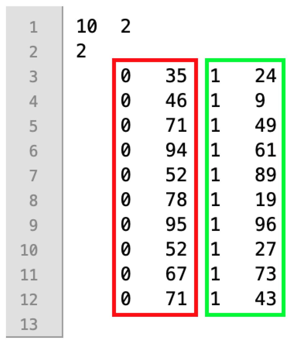

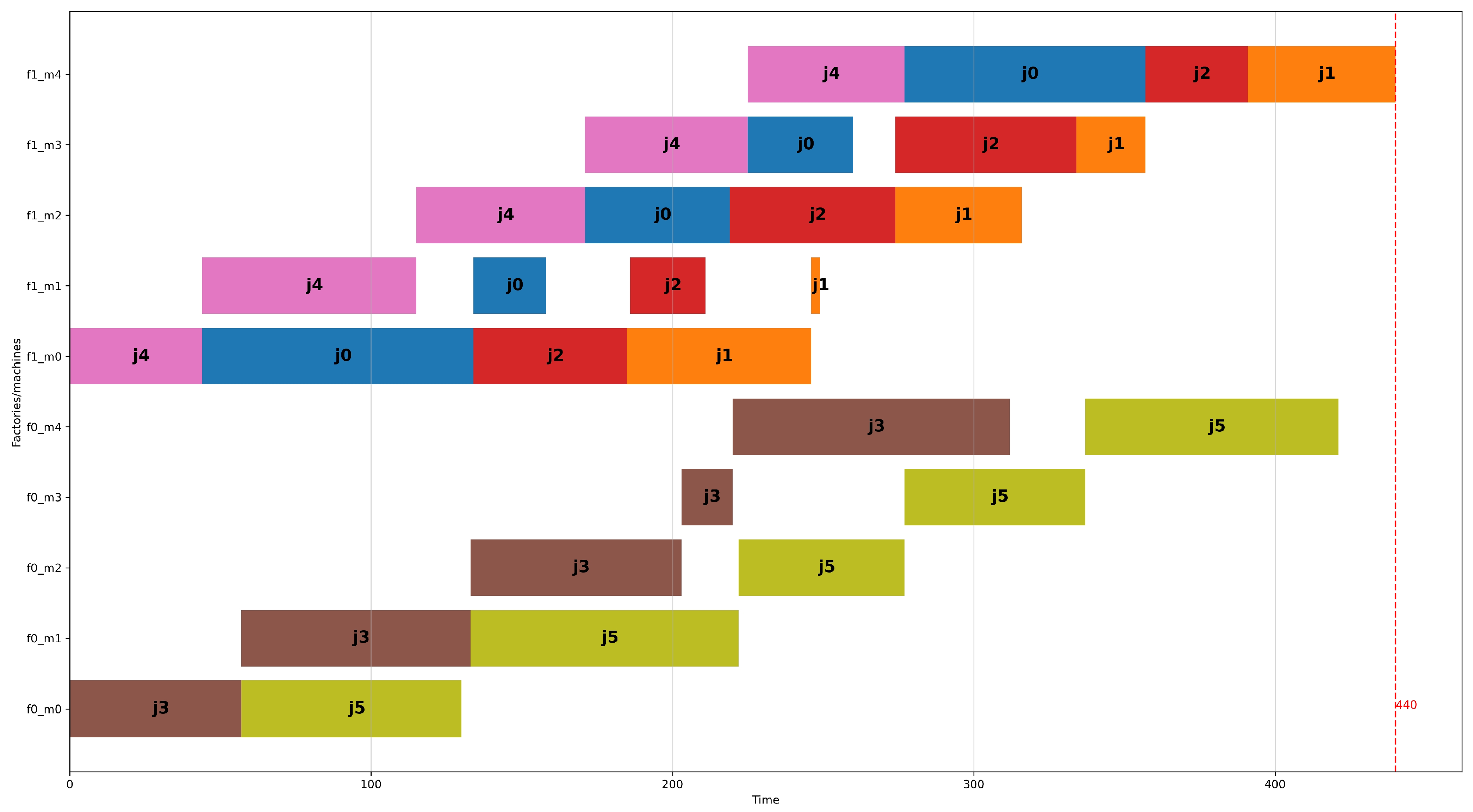

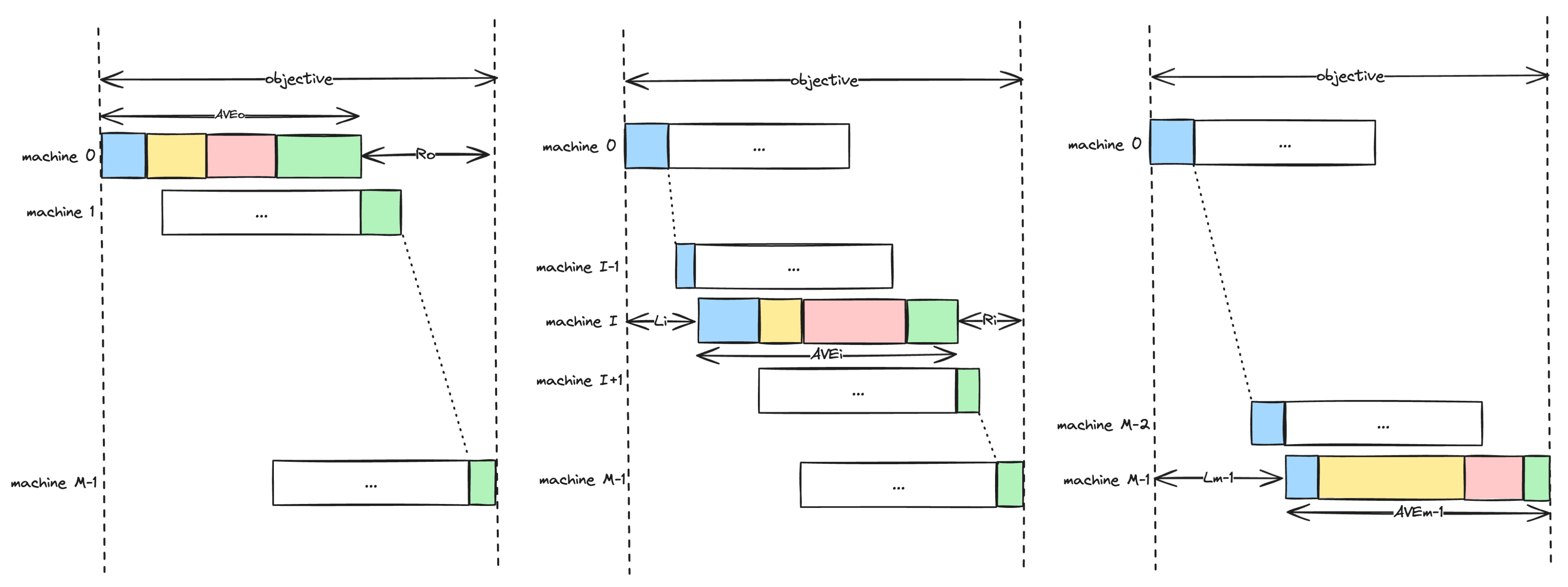
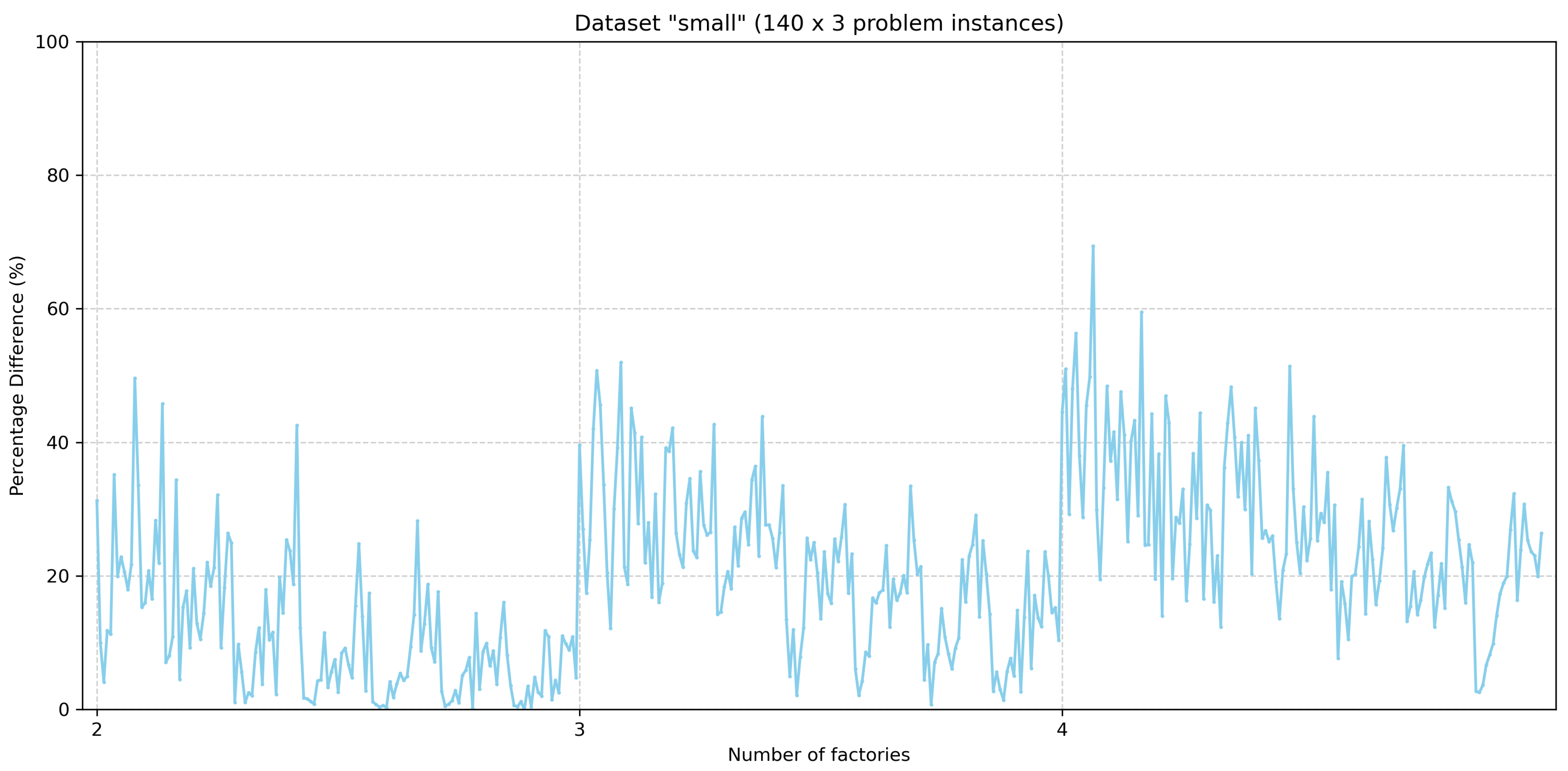
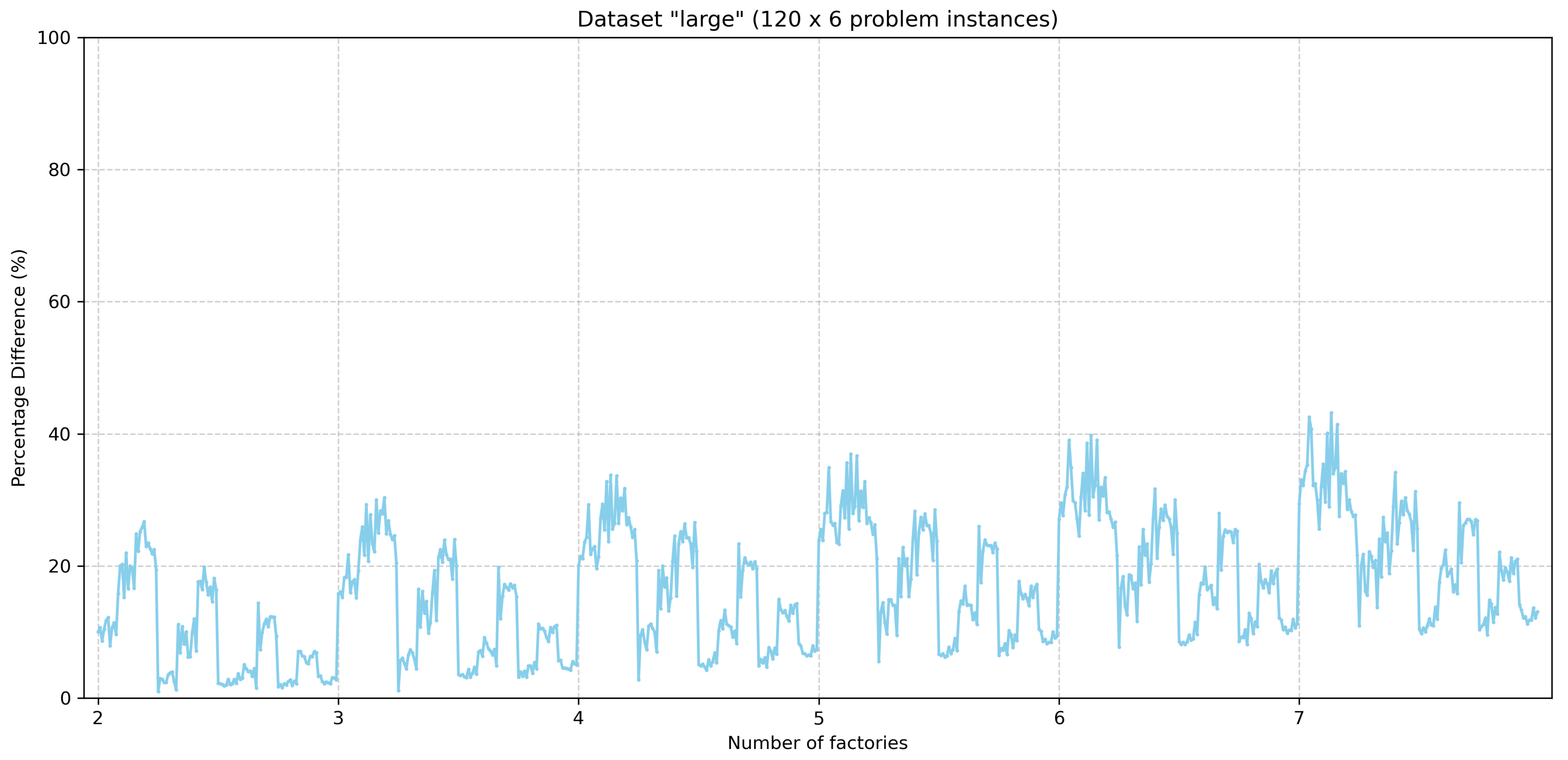
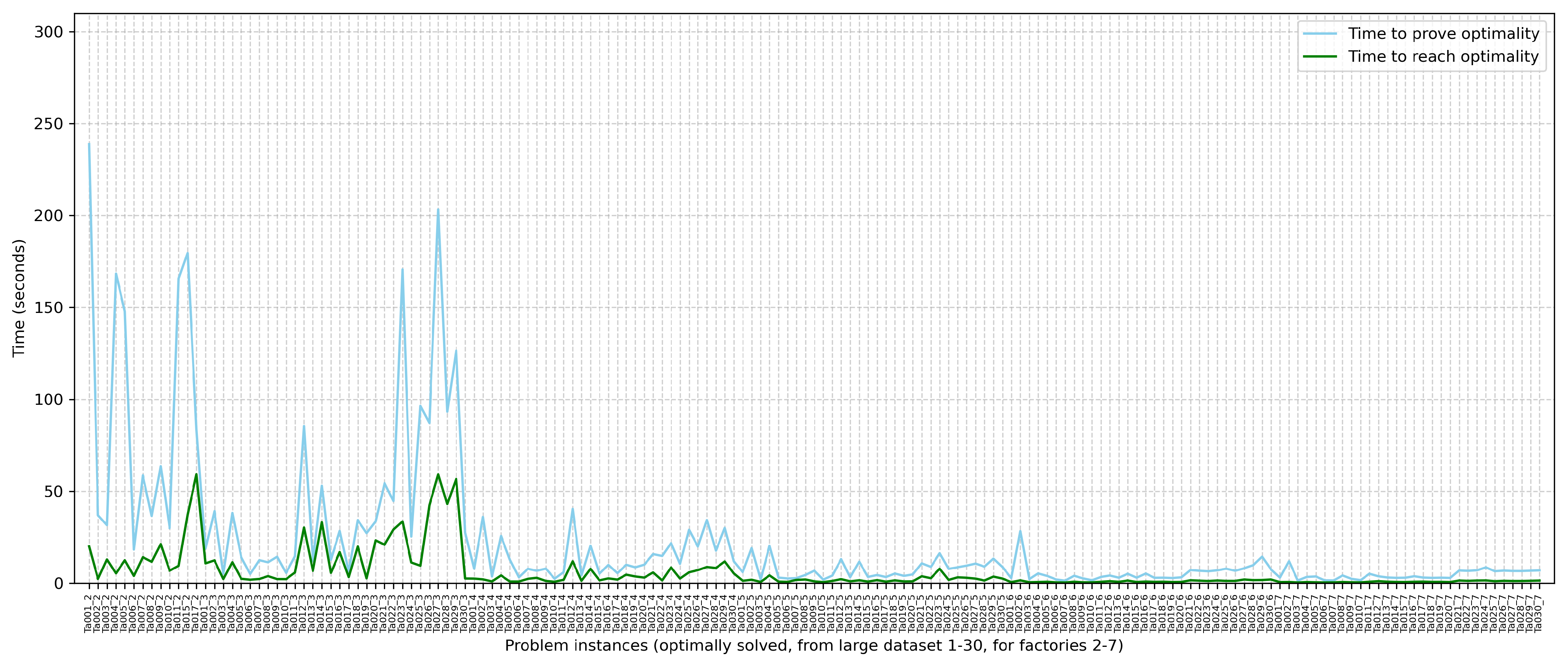
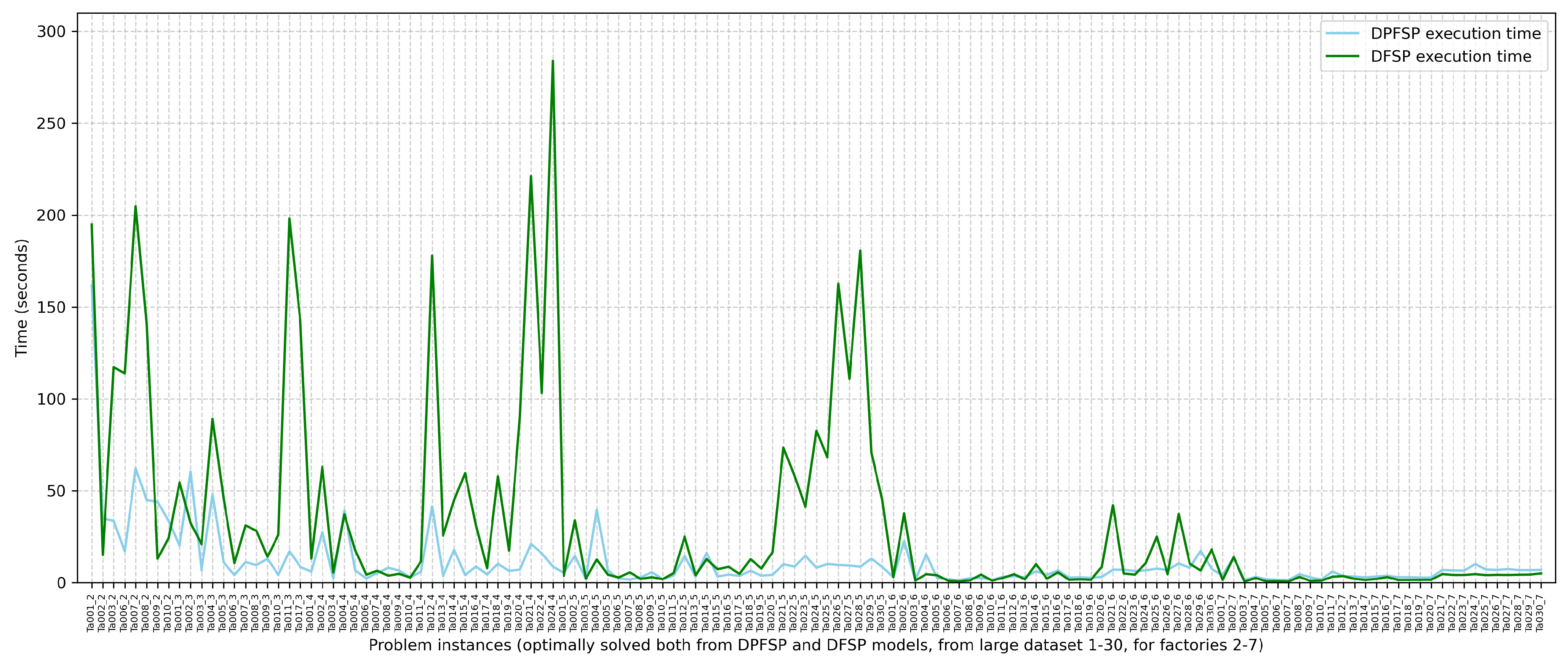
Disclaimer/Publisher’s Note: The statements, opinions and data contained in all publications are solely those of the individual author(s) and contributor(s) and not of MDPI and/or the editor(s). MDPI and/or the editor(s) disclaim responsibility for any injury to people or property resulting from any ideas, methods, instructions or products referred to in the content. |
© 2023 by the author. Licensee MDPI, Basel, Switzerland. This article is an open access article distributed under the terms and conditions of the Creative Commons Attribution (CC BY) license (https://creativecommons.org/licenses/by/4.0/).