An Improvement to the 2-Opt Heuristic Algorithm for Approximation of Optimal TSP Tour

Abstract

The travelling salesman problem (TSP) is perhaps the most researched problem in the field of Computer Science and Operations. It is a known NP-hard problem and has significant practical applications in a variety of areas, such as logistics, planning, and scheduling. Route optimisation not only improves the overall profitability of a logistic centre but also reduces greenhouse gas emissions by minimising the distance travelled. In this article, we propose a simple and improved heuristic algorithm named 2-Opt++, which solves symmetric TSP problems using an enhanced 2-Opt local search technique, to generate better results. As with 2-Opt, our proposed method can also be applied to the Vehicle Routing Problem (VRP), with minor modifications. We have compared our technique with six existing algorithms, namely ruin and recreate, nearest neighbour, genetic algorithm, simulated annealing, Tabu search, and ant colony optimisation. Furthermore, to allow for the complexity of larger TSP instances, we have used a graph compression/candidate list technique that helps in reducing the computational complexity and time. The comprehensive empirical evaluation carried out for this research work shows the efficacy of the 2-Opt++ algorithm as it outperforms the other well-known algorithms in terms of the error margin, execution time, and time of convergence.

1. Introduction

The travelling salesman problem is one of the most researched problems in the combinatorial optimisation domain [1] due to its importance and usage in different areas of daily life and many other applications. However, it is still an open challenge. Furthermore, its applications also span a variety of domains that are either formulated or generalised forms of TSP, such as circuit board printing [2], the overhauling of gas turbines [3], scheduling with deadlines [4], vehicle routing [5], and TSP with drones [6]. Due to the difficulty of solving the large instances of these problems, approximation algorithms and heuristics are the most widely used and practical approaches to obtain near-optimal solutions in a reasonable time.

Generally, the algorithm is provided with a set of cities V and the distance w between every pair of cities, and the aim of the algorithm is to find a closed tour starting from any random vertex and visiting each and every point in V with the minimum possible cost [7,8,9].

Finding the optimum solution using an exact algorithm may be very steeply priced, both in terms of time and computational resources. Complexity in this situation can reach up to $O(n!)$ because of its NP-hard nature. To cope with this problem, researchers have devised multiple heuristics and approximation techniques to find a quick and near-optimal solution [10]. The effort in finding the optimal result of any NP-hard problem can grow exponentially from huge to impossible, thus making the retrieval of a solution impractical for relatively larger-scale problem sizes [1]. Heuristics can minimise the complexity from exponential to polynomial time by sacrificing some accuracy [7]. Almost all real-world problems that rely on the effective results of TSP instances, such as network optimisation, logistics, postal, or any other industry that involves planning or logistics, can greatly benefit from the provided TSP algorithm [11,12,13].

Consider a complete graph as input to the algorithm: ${\displaystyle G=(V,E)}$ where V represents the nodes and E represents the edges. Each edge ${\displaystyle (u,v)}$∈ E has a non-negative integer cost denoted as ${\displaystyle c(u,v)}$. The problem is to find a Hamiltonian cycle (tour) of G with the minimum cost. The heuristic algorithm should solve symmetric TSP instances with a minimal error margin. It should effectively solve large-input problems in a reasonable amount of time.

The TSP can be formulated as below.

Given a set of vertices V = 0,1,2,…., n − 1, where the distance between a pair of vertices is given as $d_{ij}$, the objective is to minimise

$$\sum _i\sum _j{d}_{ij}{X}_{ij}$$

(1)

where

$$X_{ij}=\left\{\begin{array}{cc}1\hfill & \mathrm{the}\mathrm{path}\mathrm{goes}\mathrm{from}\mathrm{node}i\mathrm{to}\mathrm{node}j\hfill \\ 0\hfill & \mathrm{otherwise}\hfill \end{array}\right.$$

(2)

subject to

$$\sum _j{X}_{ij}=1$$

(3)

and each vertex needs to be visited once.

$$\sum _i{X}_{ij}=1$$

(4)

The salesman must come from only one vertex when visiting this vertex.

$$X_{ii}=0$$

(5)

There should be no self-loop.

$$\sum _i\sum _j{X}_{ij}⩽\left|S\right|-1,\forall S\subset V,2⩽\left|S\right|⩽n-2$$

(6)

We need to incorporate the global requirement that there is one tour that visits all vertices, as the local constraints defined above can lead to situations where there are multiple tours visiting only a subset of the total number n of vertices V. Here, S is a set of all possible subtours of graph G. This constraint requires that the tour should proceed from a vertex in S to a vertex not in S (and vice versa).

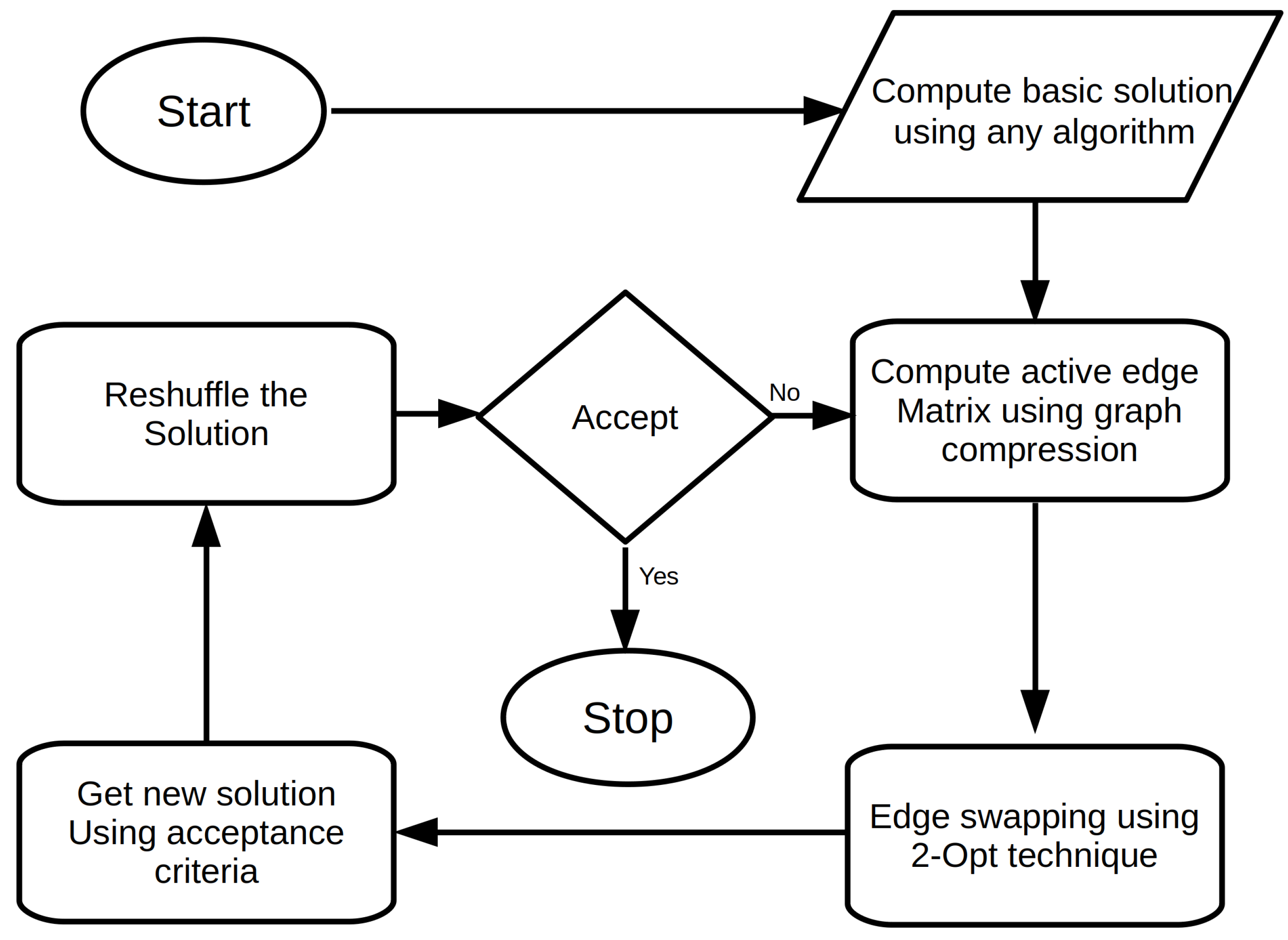
In this paper, an improved algorithm, 2OPT++, is proposed using the 2-opt technique for the TSP problem. The algorithm performs considerably well in terms of the running time and approximation ratio, even for very large problem instances. It is proposed to use an optional graph compression step to improve the running time of the algorithm when dealing with large problem instances. The approach is commonly known as the “candidate list” and results in a considerable computational performance improvement for huge graphs. An empirical comparison of the effect of utilising this technique to reduce the TSP complexity with respect to the quality of the solution is provided. A comprehensive experimental evaluation of some of the most well-known algorithms and heuristics used to solve TSP problems is provided, namely ruin and recreate, nearest neighbour, genetic algorithm, simulated annealing, Tabu search, and ant colony optimisation. Our proposed algorithm utilises an edge swap technique mixed with some carefully studied steps to generate near-optimal results. In the following, we list the steps of the 2-Opt++ algorithm; every step is further described in detail. Figure 1 shows the flow diagram of the algorithm.

• Compute a basic solution to the input problem.
• Compute an active edge matrix using the graph compression technique (optional and recommended for larger problem instances).
• Use the 2-Opt technique for edge swapping.
• Accept the new solution using acceptance criteria.
• Reshuffle the cycle and repeat until convergence or pre-defined end of iterations.

2. Existing Algorithms

A wide range of algorithms have been proposed in the literature to solve the TSP. Exact algorithms such as branch-and-bound, branch-and-cut, and cutting plane methods are guaranteed to find the optimal solution, but their running time is exponential in the worst case. Heuristic algorithms such as nearest neighbour, 2-Opt, 3-Opt, and Christofides’ algorithm provide approximate solutions in polynomial time, but the optimality of the solutions is not guaranteed. Meta-heuristics such as genetic algorithm, simulated annealing, Tabu search and ant colony optimisation are high-level strategies that can find approximate solutions quickly.

In recent years, researchers have proposed various hybrid methods that combine the advantages of different meta-heuristics with exact algorithms. These methods are considered state-of-the-art techniques to solve large-scale TSP. A number of researchers have also proposed to use meta-heuristics such as genetic algorithm, simulated annealing, Tabu search and ant colony optimisation, which can find approximate solutions quickly.

Additionally, various modifications of the TSP have been proposed in the literature, such as the asymmetric TSP (ATSP), the prize collecting TSP (PCTSP), and the multiple TSP (mTSP), which have been studied and attempted to be solved using similar approaches as in the TSP.

This section provides an introduction to some previous and well-known algorithms used to solve the travelling salesman problem.

2.1. Christofides Algorithm

In 1976, an algorithm was proposed that was guaranteed to provide a solution within a 3/2 factor of the optimal solution. The Christofides algorithm is considered one of the best algorithms due to its ease of understanding, computational complexity, and approximation ratio. This algorithm, proposed by Christofides, combines the minimum spanning tree with a solution of minimum-weight perfect matching [14,15]. In 2011, an improved version of Christofides’ algorithm was proposed for k-depot TSP, which shows a closer approximation of $2-(1/k).$ If the value of k is close to 2, the approximation bound becomes close to $3/2$ (i.e., the original approximation of Christofides).

2.2. 2-Opt and 3-Opt

Optimising the problem using smaller moves is also a very popular technique that has yielded promising results. The 2-Opt and 3-Opt algorithms are branches of local search algorithms, which are commonly used by the theoretical computer science community for the solution of the TSP [16]. The 2-Opt algorithm removes two edges from the graph and then reconstructs the graph to complete the cycle. There is always only one possibility in adding two unique edges to the graph for the completion of the cycle. If the new tour length is less than the previous one, it is kept; otherwise, it is rejected. On the other hand, 3-Opt removes three edges from the tour, resulting in the creation of three sub-tours and eight possibilities for the addition of new edges to complete the cycle again. The time complexity in 3-Opt is O(n${}^3$) for a single iteration, which is higher than for the 2-Opt algorithm. 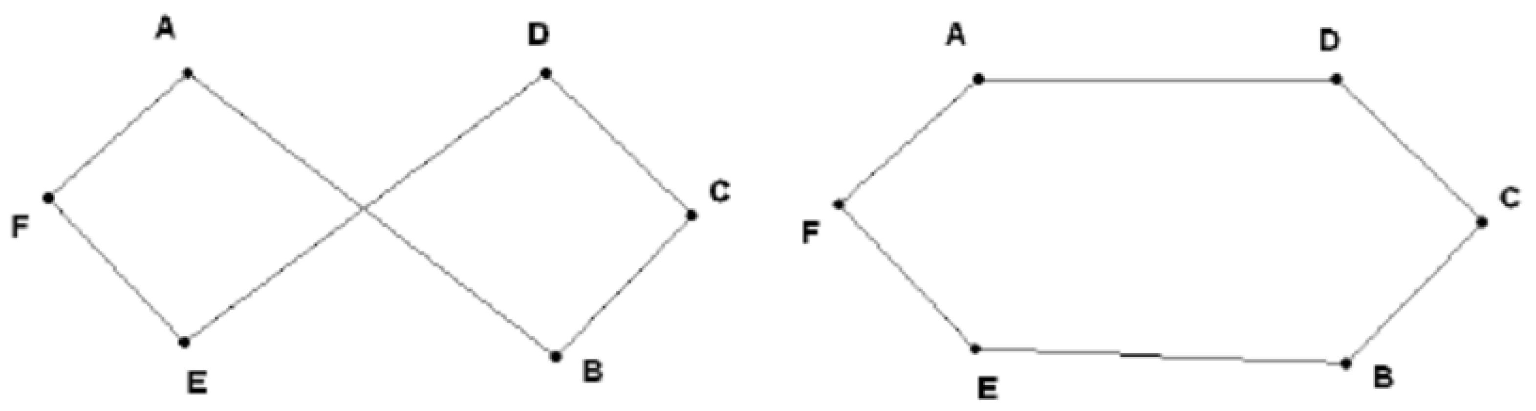Figure 3 shows the moves of the 2-Opt technique.

2.3. Nearest Neighbour

The nearest neighbour algorithm (NN) is a straightforward, greedy approximation algorithm. The tour starts with the selection of a random initial city and then incrementally adds the closest unvisited city until all cities are visited. Although this algorithm is computationally very efficient, it generally fails to provide effective results. In [10], its empirical results were compared with those of five other algorithms utilising TSPLIB problems. In this paper, we also compare the results of the 2-Opt++ algorithm with the nearest neighbour algorithm’s results. The comparison highlights that the nearest neighbour algorithm is a poor choice for TSP approximation.

2.4. Simulated Annealing

In 1983, Kirkpatrick, Gelatt, and Vecchi introduced a powerful heuristic algorithm known as simulated annealing (SA). SA is a probabilistic algorithm used to find the global optimum. The probability increases or decreases with the quality of the move. A parameter T is used to measure the probability of the move. When T tends toward zero, the probability of selection becomes more unlikely.

$$P\left(Acceptance\right)\sim 1-exp(\mathsf{\Delta }E/CT))$$

(7)

Here, C is a constant related to energy or temperature, and T is a control parameter and is set very high initially. Simulated annealing allows some poor moves to traverse through the large solution space. The acceptance of the new state is based on some predefined criteria. This process is repeated until convergence to the solution [1]. In [17], the authors claim that the threshold acceptance method is better than simulated annealing.

2.5. Genetic Algorithm

Genetic algorithm is inspired by the genetic operations of evolution, i.e., selection, crossover, and mutation. GA has been extensively used in the literature for TSP and related problems. The mutation is a key operator driving the search for a better solution. Swapping, flipping, and sliding are the main types of mutations used in GA. The idea behind genetic algorithm comes from genes, where offspring are created by exchanging the genes of their parents. Unlike other meta-heuristic methods, GA uses natural selection rules, crossover, and mutations to make the computation easier and faster. These aspects make it a more valuable, better-performing, and more efficient algorithm than others [18,19,20].

2.6. Tabu Search

Tabu search (TS) was proposed by Fred Glover in 1986 and is also known as an algorithm for neighbourhood search. Here, the search method is primarily based on the search history, denoted as Tabu listing. It is an intensive local search algorithm [21]. TS avoids the problem of becoming stuck in local optima by allowing moves with negative gains and constructing a Tabu list to inhibit contradictory moves. Whenever it becomes stuck in local optima, it searches for a solution from the neighbourhood stored in memory, even if it is worse than the currently selected one (negative gain), thus allowing it to discover more feasible options from the solution space. Here, the Tabu list helps TS to avoid cycling in the tour. TS uses 2-Opt moves to enhance the solution. However, TS is slower than other 2-Opt local search algorithms.

2.7. Ant Colony Optimisation

Machine learning scientist Marco Dorigo, in 1993, outlined a strategy to heuristically solve TSP by deploying a technique involving the recreation of a subterranean insect province called the Ant Colony System (ACS). It uses the analogy that genuine ants discover short paths between sustainable sources and their homes. As ants are blind, they start navigating towards the food source from their colony and deposit pheromones along the path. Every ant searches and follows the path at random. The probability of following a path increases with the increase in pheromones in the path. The algorithm uses artificial ant behaviour, and it records their location and the quality of the solution so that this path can be checked for acceptance or rejection in future iterations. The measure of pheromone storage corresponds to the visit length: the shorter the visit, the more it stores [22,23]. In their work, Leila Eskandari and Ahmad Jafarian [24] argue that ACO is one of the most efficient nature-motivated meta-heuristic algorithms and has outperformed a considerable number of algorithms in this domain. They have modified and improved the ACO algorithm to devise another strategy to solve TSP. In essence, they compare both local and global solutions to find the best possible solution. In [22], the authors use Tabu listing to avoid the repetition of path selection in ant colony optimisation, which considerably improves the overall algorithm’s time and convergence.

2.8. Tree Physiology Optimisation

An important property in nature is sustainability and continuous improvement for survival. This unique property reflects the pattern of optimisation. TPO is an algorithm influenced by a tree development scheme that uses the shoot and root feature to achieve optimal survival. The shooting system expands to a light source in ordinary plant growth to capture light and initiate the photosynthesis process. The method of photosynthesis transforms light into carbon with the assistance of water, which is then provided and used by other components of the plant; specifically, the root system uses oxygen to elongate shooting in the opposite direction. It consumes carbon to further elongate inside the floor for water and nutrient searching, which is then provided to the shooting extension system. The shoot–root system’s connection to ideal development can be converted by a straightforward concept into an optimisation algorithm; the shoot searches for carbon using root nutrients, and the root searches for nutrients using the shooting system. In [10], TPO results are compared with those of five other algorithms.

2.9. Ruin and Recreate

R&R is a simple but powerful meta-heuristic used to solve combinatorial optimisation problems. The ruin and recreate (R&R) method uses the concepts of simulated annealing or threshold acceptance, with massive actions in place of smaller ones. As the name suggests, a large chunk of the problem is ruined and recreated. Complex problems such as timetable scheduling or vehicle routing problems, which are often discontinuous, require large moves to bypass the local optima. The R&R algorithm has proven to be an important candidate to find the global optimum. The vehicle routing problem using R&R is discussed in detail in [25]. A case study using R&R is presented in [26]. There is a fleet of vehicles that has to serve different numbers of customers. There is a central depot where the route of each vehicle starts and ends. Vehicles need to serve customers that have certain demands. The idea is to serve the customers with the minimum route (distance travelled) and within the capacity of every vehicle assigned to it. A time window constraint can also be added to the problem, i.e., every customer can add a start and end time to their service. A total of 56 problems have been studied in this paper and the results are discussed. Jsprit is an implementation of the R&R algorithm presented in [25], and it is available for download (https://github.com/graphhopper/jsprit (accessed on 3 May 2023)) and use.

We have used the above implementation to benchmark the problems from TSPLIB and compared the results with those of the 2-Opt++ algorithm. In this study, R&R performed considerably well in terms of the error margin and convergence in some problems.

3. 2-Opt++ Algorithm

3.1. Basis for Solution

Initially, the algorithm needs to be provided with a Hamiltonian cycle as a base input. A random Hamiltonian cycle is quickly computed by using a greedy technique (least cost edge) and then an edge swap technique is used to iteratively improve upon the original tour. It is pertinent to mention that although we have computed the Hamiltonian cycle in a greedy manner for this work, any method can be utilised to compute the Hamiltonian cycle, as the effectiveness of the 2-Opt++ algorithm is beneficial in cases where the initial Hamiltonian cycle is of higher quality in terms of the total edge weight. However, it is not entirely dependent on such optimistic scenarios only, as the proposed edge swap technique and the graph compression/candidate list are also key to the 2-Opt++ algorithm’s success.

3.2. Graph Compression (Optional)

Also known as a candidate list, for each graph, a $N\times N$ matrix is initialised with 0s, where N is the number of nodes in the graph. The nearest k points are identified and these points are considered active for the node v${}_i$∈ V and are marked 1 in the active edge matrix. Only active edges are considered and compared in the algorithm. This step is optional and is recommended for larger instances of TSP to save time. Here, 100 active edges (i.e., $k=100)$ are considered in solving large problem instances.

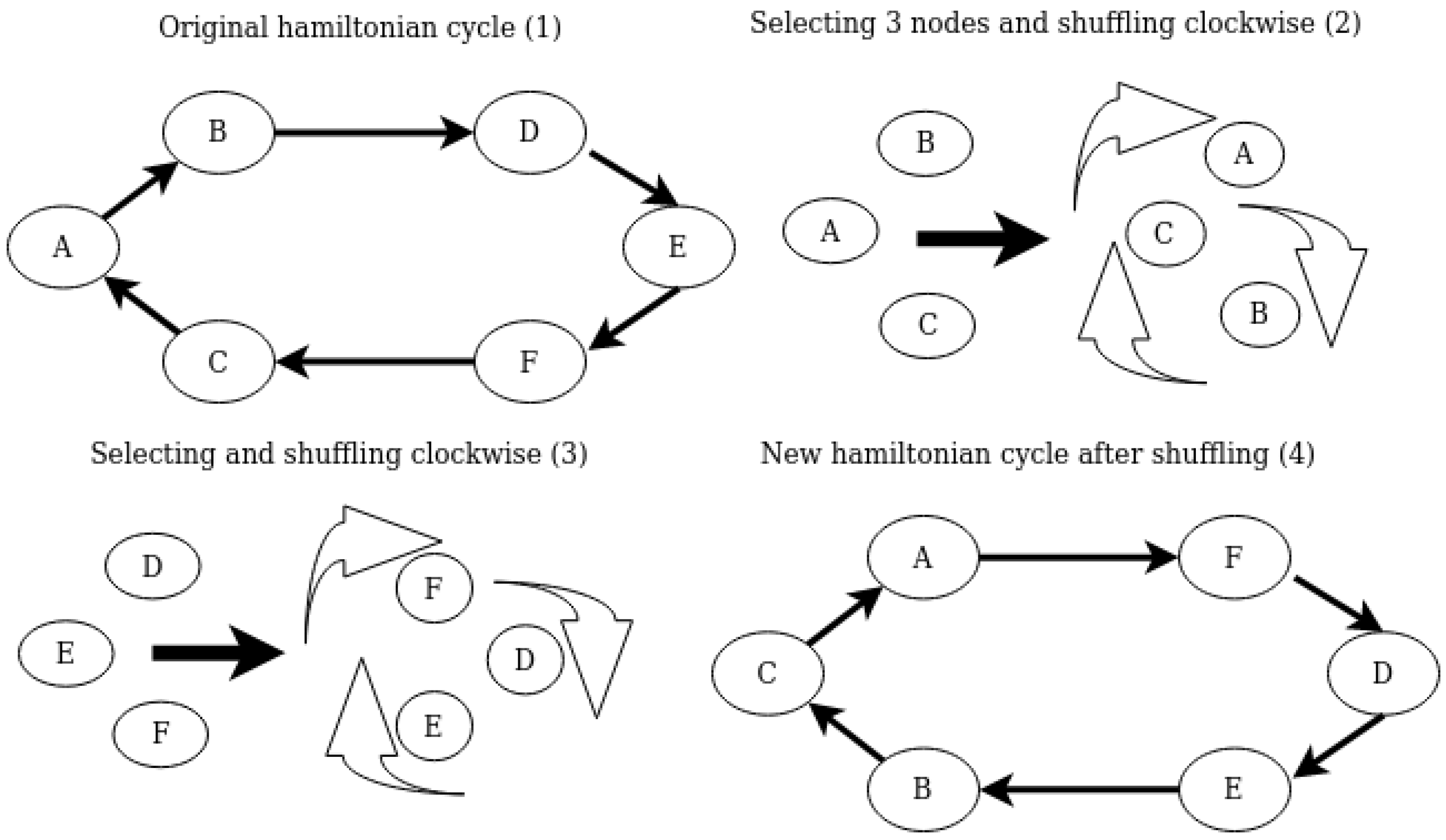
3.3. Shuffling

The next step is to shuffle the original Hamiltonian cycle generated in the first step. The algorithm selects a group of three nodes from the original cycle and then processes them in a clockwise direction in two steps. We would like to highlight that although it is possible to select a variable number of nodes and steps, we have selected a combination of 3 nodes and 2 steps after an extensive evaluation with different combinations of numbers of nodes and steps, as shown in Figure 2.

3.4. Mutation

Different techniques have been used for mutation in different algorithms, and Lin–Kernighan is a well-known one that removes two, three, four, or five connections from the graph and then selects a new solution from 2, 4, 25, or 208 different possible scenarios [8]. In this article, we have applied a simple mutation. We remove two edges from the complete Hamiltonian cycle H and revert them and reconnect them again to create a new solution. This is the same technique used in the Lin-2-Opt method [16].

Suppose that we have two edges AD and EB, shown in Figure 3. We remove these two edges from the graph and add two more edges as AB and ED to complete the graph.

3.5. Gain Computation

The total weight of this newly computed graph will be calculated again, and if the new sum of the weight is smaller than the previous one, the distance is minimised from the previous value and new edges will be accepted; otherwise, they will be rejected. This step will be repeated for every edge in the graph of the respective node.

Let x be the distance from node A to node D from Figure 3 and $\overline{x}$ be the distance from node E to node B. In the case of a symmetric graph, the distance from A to D and D to A will be identical. Let y be the distance from node A to node B and $\overline{y}$ be the distance from node E to node D. Then, we have a gain as

$$Gain=R_n-R_p$$

(8)

Here, let $R_n$ be the sum of the edge distance that is to be added to the new graph, i.e., $R_n$ = $y+\overline{y}$, while $R_p$ is the sum of the edge distance that is to be removed, i.e., $R_p$ = $x+\overline{x}$ (Algorithm 1).

Algorithm 1 2-Opt++

3.6. Selection Criteria

Reverting the edges and then testing for an improved solution is a simple yet powerful method. However, there is a caveat in this solution. As we are checking for every suitable solution and then adapting it in a greedy manner, it raises the possibility of missing a better solution. This point can be improved in the future by defining some criteria for the possible acceptance of a solution, e.g., simulated annealing accepts any better solution with a certain probability measure [1]; moreover, in the threshold acceptance method, results are accepted if they satisfy certain threshold values [17]. If the gain in the previous step is greater than 0, we will keep this new solution. The 2-Opt++ algorithm is fully explained above 1.

4. Experimental Results and Analysis

In this section, we present a detailed evaluation of the 2-Opt++ algorithm using multiple resources and provide a performance comparison with some of the other well-known algorithms selected from the literature. We have mainly benchmarked TSPLIB examples to test the efficiency of our algorithm and have compared it with the $R\&R$ algorithm and some other well-known algorithms/heuristics selected from the existing literature, such as nearest neighbour, Tabu search, simulated annealing, genetic algorithm, and ant colony optimisation. We have selected 67 symmetric problems from the well-known TSPLIB library, as shown in

Table 1. Problems selected from the library TSPLIB for benchmarking.

No.	Name	Nodes	Opt.	No.	Name	Nodes	Opt.
1	eil51	51	426	35	a280	280	2579
2	berlin52	52	7542	36	pr299	299	48,191
3	st70	70	675	37	lin318	318	42,029
4	eil76	76	538	38	rd400	400	15,281
5	pr76	76	108,159	39	fl417	417	11,861
6	rat99	99	1211	40	pr439	439	107,217
7	kroa100	100	21,282	41	pcb442	442	50,778
8	krob100	100	22,141	42	d493	493	35,002
9	kroc100	100	20,749	43	u574	574	36,905
10	krod100	100	21,294	44	rat575	575	6773
11	kroe100	100	22,068	45	p654	654	34,643
12	rd100	100	7910	46	d657	657	48,912
13	eil101	101	629	47	u724	724	41,910
14	lin105	105	14,379	48	rat783	783	8806
15	pr107	107	44,303	49	pr1002	1002	259,045
16	pr124	124	59,030	50	u1060	1060	224,094
17	bier127	127	118,282	51	vm1084	1084	239,297
18	ch130	130	6110	52	pcb1173	1173	56,892
19	pr136	136	96,772	53	d1291	1291	50,801
20	pr144	144	58,537	54	rl1304	1304	252,948
21	ch150	150	6528	55	rl1323	1323	270,199
22	kroa150	150	26,524	56	fl1400	1400	20,127
23	krob150	150	26,130	57	u1432	1432	152,970
24	pr152	152	73,682	58	fl1577	1577	22,249
25	u159	159	42,080	59	d1655	1655	62,128
26	rat195	195	2323	60	vm1748	1748	336,556
27	d198	198	15,780	61	u1817	1817	57,201
28	kroa200	200	29,368	62	rl1889	1889	316,536
29	krob200	200	29,437	63	d2103	2103	80,450
30	ts225	225	126,643	64	pr2392	2392	378,032
31	tsp225	225	3916	65	fl3795	3795	28,772
32	pr226	226	80,369	66	pla33,810	33,810	66,048,945
33	gil262	262	2378	67	pla85,900	85,900	142,382,641
34	pr264	264	49,135	-	-	-	-

.

We have rigorously evaluated the 2-Opt++ algorithm and present our findings in this section, with a detailed comparison with $R\&R$ and six other algorithms/heuristics. Jsprit is an implementation of the ruin and recreate algorithm [25]. We have empirically tested the $R\&R$ algorithm by using TSPLIB problems, and the results obtained are presented in

Table 2. Comparison of 2-Opt++ algorithm with $R\&R$ in time and error.

Name	Opt.	R&R			2-Opt++ Algorithm
		Best	Err %	Sec	Best	Err %	Sec
berlin52	7542	7820.80	3.70	5.7	7544.26	0.03	0.12
bier127	118,282	127,550.90	7.84	30.2	119,228.26	0.8	0.58
ch150	6528	6712.87	2.83	52.4	6683.37	2.38	1.00
d198	15,780	15,937.39	1.00	74	16,160.30	2.41	1.85
d493	35,002	35,923.41	2.63	258	36,479.08	4.22	14.21
eil101	629	662.89	5.39	15.2	666.93	6.03	0.31
eil51	426	444.42	4.32	2.5	432.35	1.49	0.08
eil76	538	573.28	6.56	6.6	553.01	2.79	0.17
fl417	11,861	13,094.38	10.40	207	12,061.45	1.69	8.46
gil262	2378	2422.93	1.89	108	2462.66	3.56	2.63
kroa100	21,282	21,559.42	1.30	15.8	21,522.49	1.13	0.31
kroa150	26,524	26,952.53	1.62	46.8	26,635.40	0.42	0.77
kroa200	29,368	30,231.95	2.94	73	30,031.72	2.26	1.39
krob100	22,141	22,746.89	2.74	15	22,295.99	0.7	0.33
krob150	26,130	26,237.26	0.41	48	26,568.98	1.68	0.76
kroc100	20,749	21,154.50	1.95	15	20,815.40	0.32	0.36
krod100	21,294	21,842.21	2.57	17.5	21,813.57	2.44	0.31
kroe100	22,068	22,413.32	1.56	14.8	22,299.71	1.05	0.34
pr107	44,303	63,228.97	42.72	19	46,066.26	1.08	0.41
pr124	59,030	70,108.17	18.77	26	59,667.52	1.24	0.71
pr136	96,772	104,690.06	8.18	36	97,971.97	2.25	0.84
pr144	58,537	69,368.47	18.50	42	59,854.08	0.46	0.84
pr152	73,682	79,805.00	8.31	46	74,020.94	2.11	0.96
pr226	80,369	88,804.29	10.50	99	82,064.79	0.82	2.28
pr264	49,135	58,608.78	19.28	105	49,537.91	3.78	3.75
pr299	48,191	53,950.30	11.95	116	50,012.62	3.27	4.71
pr439	107,217	120,717.01	12.59	188	110,723.00	1.83	11.63
pr76	108,159	110,467.08	2.13	6.5	110,138.31	0.94	0.23
rat195	2323	2378.49	2.39	67	2344.84	6.68	1.80
rat99	1211	1231.29	1.68	13	1291.89	1.65	0.40
rd100	7910	8046.29	1.72	14.8	8040.52	1.12	0.38
st70	675	693.37	2.72	5.2	710.51	1.96	0.21
ts225	126,643	142,681.07	12.66	82.5	129,125.20	1.38	2.28
tsp225	3916	4371.03	11.62	83.2	3970.04	3.52	2.27
u159	42,080	49,734.95	18.19	47	43,561.22	2.51	0.93

, along with the results of the 2-Opt++ algorithm. The comprehensive comparative analysis of the 2-Opt++ algorithm with existing algorithms, i.e., nearest neighbour (NN), genetic algorithm (GA), simulated annealing (SA), Tabu search (TS), ant colony optimisation (ACO), and tree physiology optimisation (TPO), are provided in

Table 3. Comparison of 2-Opt++ algorithm with existing algorithms.

N0.	TSP Instance	Error %
		TPO	NN	GA	SA	TS	ACO	2-Opt++
1	eil51	2.64	18.56	6.60	3.08	3.08	9.73	2.37
2	berlin52	2.17	8.50	5.36	5.55	2.63	5.04	0.03
3	st70	3.28	12.82	3.81	3.16	2.26	12.08	1.96
4	eil76	3.49	13.80	5.95	5.42	4.41	9.78	2.87
5	pr76	5.26	21.05	13.70	4.48	1.64	9.78	0.94
6	ch150	6.35	8.42	7.30	8.18	5.12	12.60	2.54
7	a280	7.89	19.98	8.82	9.74	8.60	11.20	6.29
8	rd400	19.04	19.23	8.42	10.05	35.62	26.03	5.89
9	pcb442	19.64	16.10	9.73	13.08	63.70	24.93	3.98
10	rat99	4.53	13.03	6.16	5.48	2.68	9.36	2.79
11	eil101	7.31	17.01	9.04	6.86	6.14	19.70	6.27
12	d198	5.49	14.46	5.09	3.81	1.92	14.27	2.74
13	kroA100	5.55	16.05	6.79	4.68	5.82	7.80	1.13
14	ch130	6.63	17.82	8.20	7.34	9.94	13.16	2.34

. We also present the performance of 2-Opt++ for larger TSP problem instances in

Table 4. Error comparison of 2-Opt++ algorithm with nearest neighbour drawn by graph compression technique in all categories.

No.	Name	2-Opt++	NN	No.	Name	2-Opt++	NN
1	eil51	2.65	18.56	34	fl3795	6.21	18.95
2	berlin52	0.03	8.50	35	a280	6.03	19.98
3	st70	3.08	12.82	36	pr299	2.05	24.3
4	eil76	5.3	13.80	37	lin318	3.16	28.56
5	pr76	0.56	21.05	38	rd400	6.32	19.23
6	rat99	2.99	13.03	39	fl417	1.69	27.43
7	kroa100	1.13	16.05	40	pr439	6.79	22.45
8	krob100	0.71	31.68	41	pcb442	5.24	16.10
9	kroc100	0.32	26.89	42	d493	4.64	24.7
10	krod100	2.44	26.56	43	u574	4.69	27.03
11	kroe100	1.15	25.01	44	rat575	8.02	24.75
12	rd100	1.13	25.68	45	p654	3.45	25.31
13	eil101	6.19	17.01	46	d657	5.01	27.12
14	lin105	1.38	41.61	47	u724	8.02	31.77
15	pr107	0.89	5.36	48	rat783	7.96	27.81
16	pr124	1.07	17.4	49	pr1002	5.34	21.83
17	bier127	0.87	14.77	50	u1060	5.02	25.68
18	ch130	2.55	17.82	51	vm1084	5.49	25.98
19	pr136	2.32	24.81	52	pcb1173	7.37	23.53
20	pr144	0.53	5.32	53	d1291	7.31	17.99
21	ch150	2.68	8.42	54	rl1304	4.94	34.33
22	kroa150	2.95	26.71	55	rl1323	5.41	22.91
23	krob150	1.67	25.62	56	pr2392	7.74	22
24	pr152	4.32	16.31	57	fl1400	4.1	34.01
25	u159	3.37	29.92	58	u1432	8.06	23.43
26	rat195	6.94	18.9	59	fl1577	3.72	25.58
27	d198	2.22	14.46	60	d1655	8.14	20.55
28	kroa200	3.72	21.9	61	vm1748	6.43	21.25
29	krob200	2.25	25.63	62	u1817	7.92	24.3
30	ts225	2.29	20.41	63	rl1889	4.49	26.58
31	tsp225	3.25	23.31	64	d2103	5.27	8.72
32	pr226	0.66	17.81	65	pla33,810	9.24	17.08
33	gil262	3.26	36.31	66	pla85,900	10.14	22.23

.

4.1. Parameter Settings and Machine Configuration

In the 2-Opt++ algorithm, there are two main variables, $N^{itr}$ and $K^{itr}$. $N^{itr}$ is set for shuffling the Hamiltonian cycle after every mutation cycle, while $K^{itr}$ is set for the number of mutation cycles. Thus,

$$TotalNumberofIterations=N^{itr}\times K^{itr}$$

(9)

We have divided the benchmark problems shown in Table 1 into three categories from the library, i.e., small, medium, and large. Small problems are in the range of (50 < n ≤ 500), medium benchmark problems have a range of (500 < n ≤ 5000), and large problems have a range of (n > 5000). We have defined 2000 iterations for the small category, 500 iterations for the medium category, and 50 iterations for the large category. The $R\&R$ results have also been generated by running the algorithm on 2000 iterations for the sake of fairness. The authors that have published results for other algorithms, i.e., NN, GA, SA, TS, ACO, and TPO algorithms, have opted for a minimum of 10,000 iterations for each algorithm [10]. For the convergence graph, every problem has been iterated 10, 100, 500, 1000, and 2000 times and the corresponding result has been recorded. All the empirical results have been computed by running the 2-Opt++ algorithm and $R\&R$ on an i7 core, 6600U CPU @ 2.60 GHz * 2, machine having 16 GB RAM and a 64-bit operating system.

4.2. Experiment with $R\&R$

In this section, we present the experimental results of the 2-Opt++ algorithm along with the results of the well-known ruin and recreate algorithm implemented as Jsprit using similar settings [25]. Each test case involved 10, 100, 500, 1000, and 2000 iterations to draw the graph for convergence. We ran both algorithms a fixed number of times for every TSP problem. Moreover, we also recorded the time taken by each algorithm to provide the results for each problem.

In the case of the 2-Opt++ algorithm, for small problems comprising 50 to 500 nodes, we decided to run the algorithm on 2000 iterations and with a full active matrix, which means that each and every node was active in the graph. In Table 2, we provide the results after experimenting on both algorithms with the details of individual TSP problems. The error formula is defined as

$$Error=\left(\right(result-opt)/opt)\times 100$$

(10)

In 29 out of 35 selected benchmarked problems, belonging to the small category, the 2-Opt++ algorithm performed better than $R\&R$. In six problems, $R\&R$ outperformed the 2-Opt++ algorithm. However, a key aspect of the 2-Opt++ algorithm in comparison to $R\&R$ is that the error variance never increases more than $7\%$, while the $R\&R$ algorithm produces a sub-par 42.7% error margin for the problem pr107. It is also evident from the results that there are many cases where the error percentage of the results produced by $R\&R$ is more than 18%. Moreover, if we look at the execution time factor, the 2-Opt++ algorithm outperforms $R\&R$ by a fair margin while still producing notably better results for all the tested problems. It is also worth mentioning that after applying graph compression for up to 100 nodes, i.e., $k=100$, the time taken by the 2-Opt++ algorithm is improved even further. It is also shown in Figure 5, that the $R\&R$ algorithm performed so poorly in terms of the computation time for the larger problems that we had to abort the computation of results for larger problems for comparison’s sake. However, we recorded the results for the 2-Opt++ algorithm for all categories and they are presented in Table 4, for future reference.

4.3. Performance Comparison

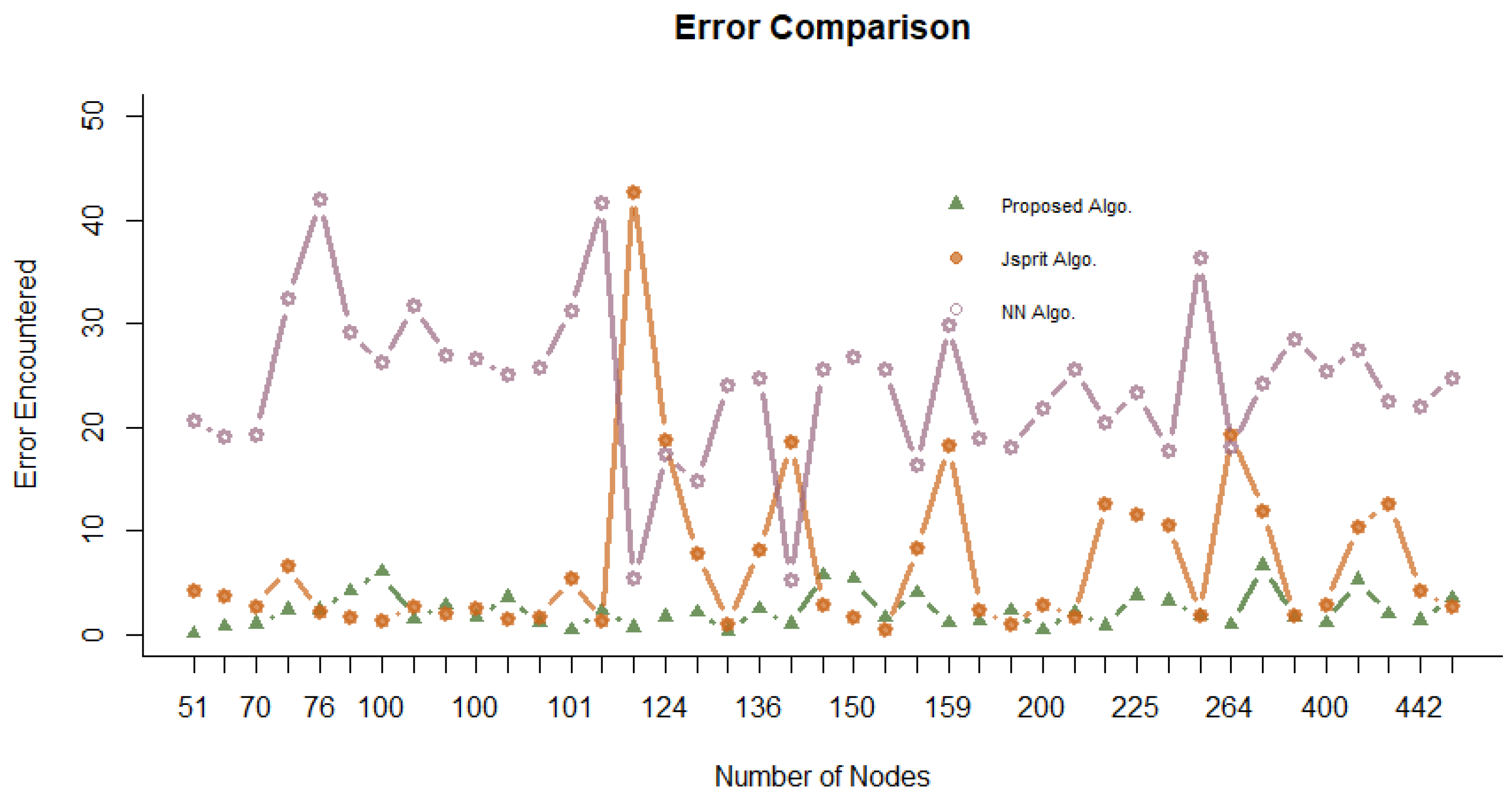
The graph of Figure 4 depicts the error margin in the three algorithms, i.e., 2-Opt++, NN, and $R\&R$ algorithms, for the small category. It is evident that the 2-Opt++ algorithm outperforms the two other algorithms most of the time, and $R\&R$ performs comparatively better than NN. However, it is also worth noting that, in some cases, the $R\&R$ algorithm yielded results that were even worse than NN, and the variance in the error margin from $R\&R$ was also considerably higher. On the other hand, the 2-Opt++ algorithm produced better and more consistent results and never exceeded the acceptable margin of 7% for problems belonging to the small category.

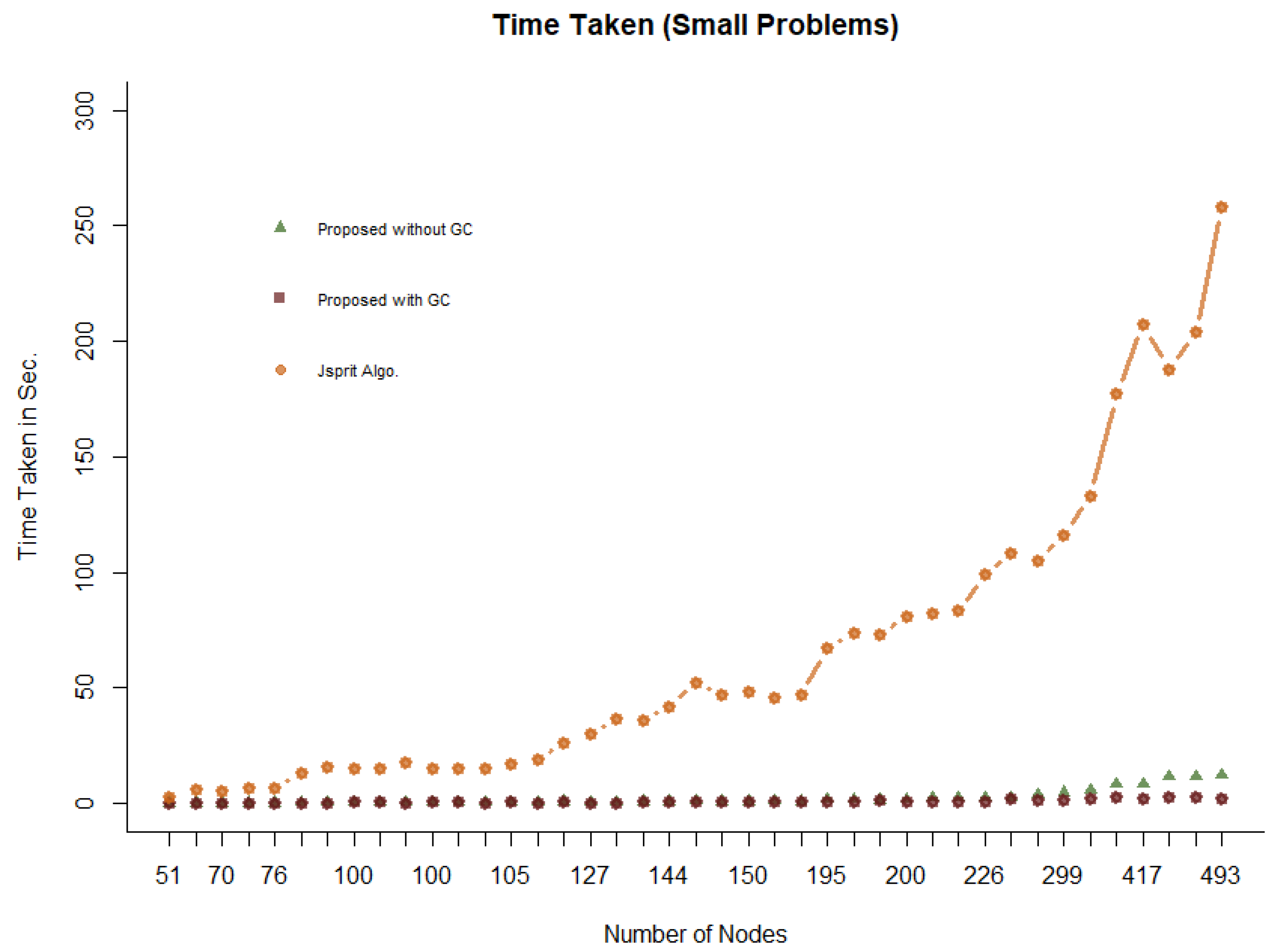
Figure 5 provides a graphical comparison of the time consumed by the $R\&R$ and 2-Opt++ algorithms in the small category. The results highlight the superiority of our proposed algorithm in terms of the computational time. It is pertinent to mention that the computational time consumed by the 2-Opt++ algorithm is impressive even for considerably larger problems. The computational time performance was improved further after applying the graph compression technique. The graph clearly showed an abrupt increase in the time taken by the $R\&R$ algorithm for problems with an increasing number of nodes.

4.4. Comparison with Other Algorithms/Heuristics

In this section, we elaborate and compare the results of six other well-known algorithms/heuristics with the 2-Opt++ algorithm and highlight the key findings. In the original comparative study [10], the authors selected some parameters, such as the number of iterations and number of experiments with each algorithm. The minimum number of iterations was selected as 10,000. Each algorithm continued its execution until it reached the already published results or completed the defined number of iterations.

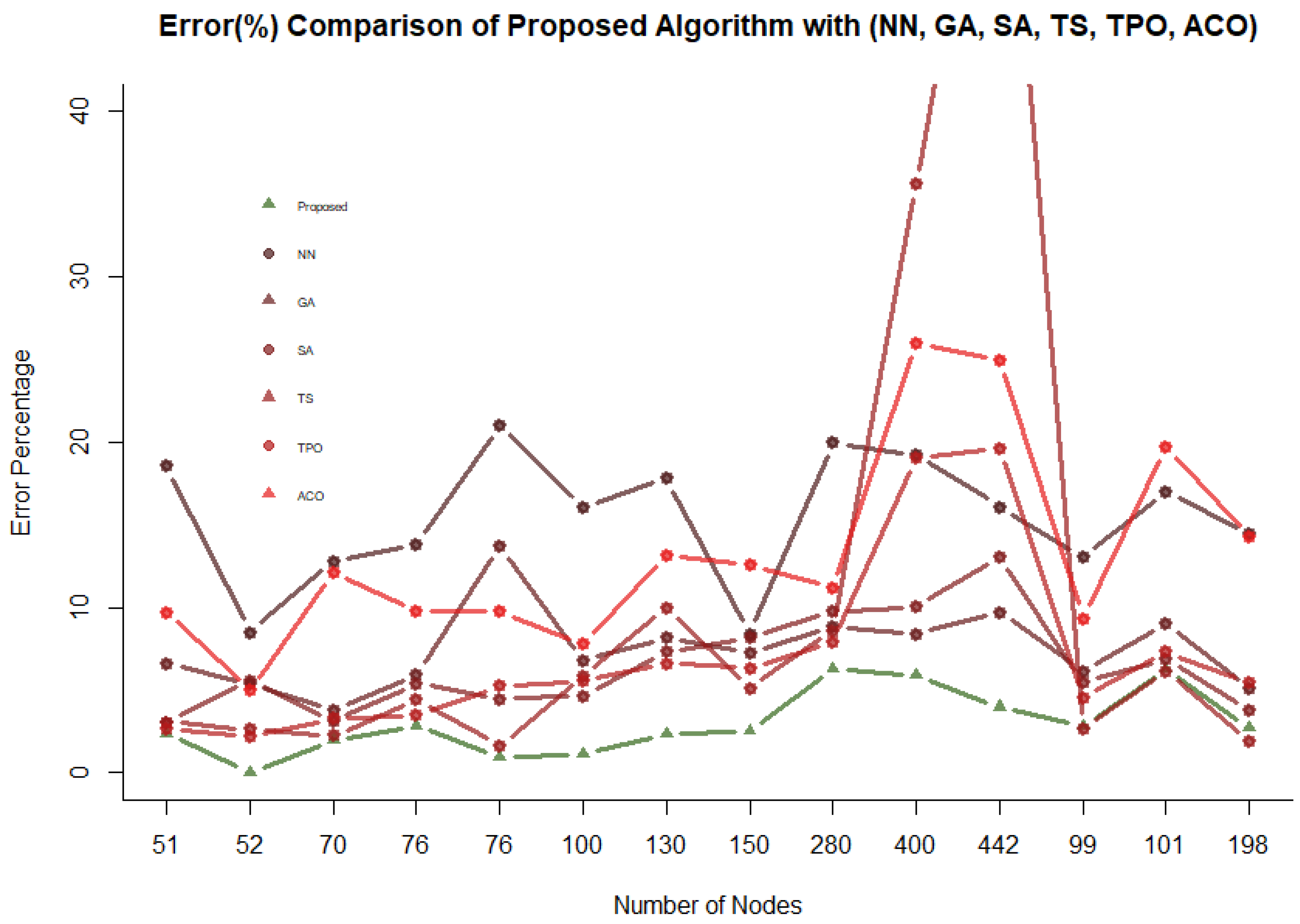
In Table 3, we present the resultant error margins of the six selected algorithms along with the results of the 2-Opt++ algorithm. Each problem was evaluated with 2000 iterations of the 2-Opt++ algorithm. Table 3 provides the error percentages of all the algorithms using a simple, basic formula for the error percentage, i.e., $\left(\right(best-opt)/opt)\times 100$. It is clearly evident that the results of the 2-Opt++ algorithm are superior and it is more effective than the other algorithms in terms of the error percentage.

Out of the 14 problems, our proposed algorithm yielded the best results for 11 problems, and, even for the other three problems, the difference was minimal. In problem rat99, Tabu search provided a better solution, with an error percentage of 2.68%, while the 2-Opt++ algorithm yielded a 2.79% error rate. However, when we regenerated our results with the graph compression technique using only 40 active edges, our algorithm produced a much improved error rate of 2.26%, even outperforming the initially best-performing Tabu search. For the problem eil101, Tabu search provided a 6.14% error rate, while the 2-Opt++ algorithm showed a 6.27% error rate. However, again, when we applied the graph compression technique, the 2-Opt++ algorithm was able to surpass Tabu search, with an error rate of 5.63%. For the problem d198, Tabu search showed an error margin of 1.92% and the 2-Opt++ algorithm produced a 2.74% error. Again, after reproducing the results with graph compression, i.e., setting the active edges to 40, we were able to produce a 1.49% error rate.

It is clearly evident that the 2-Opt++ algorithm performs well for more than 80% of the cases in normal execution, and, even for the rest of the cases, our algorithm is able to outperform the others in terms of the error percentage with the introduction of the graph compression technique.

Figure 6 depicts a graphical comparison of the error margins of the seven different algorithms. The graph clearly shows the impressive performance of the 2-Opt++ algorithm.

4.5. Qualitative Results

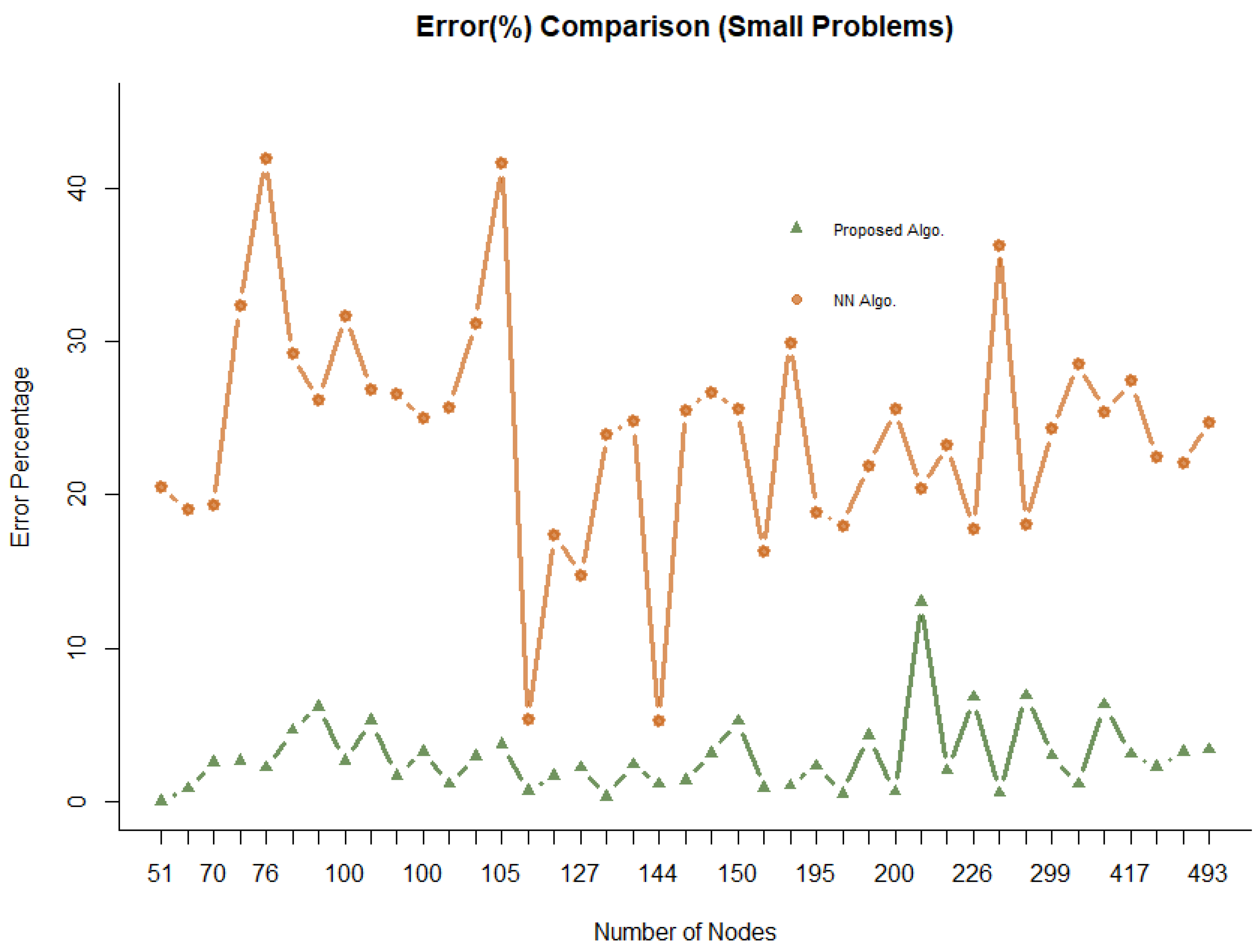
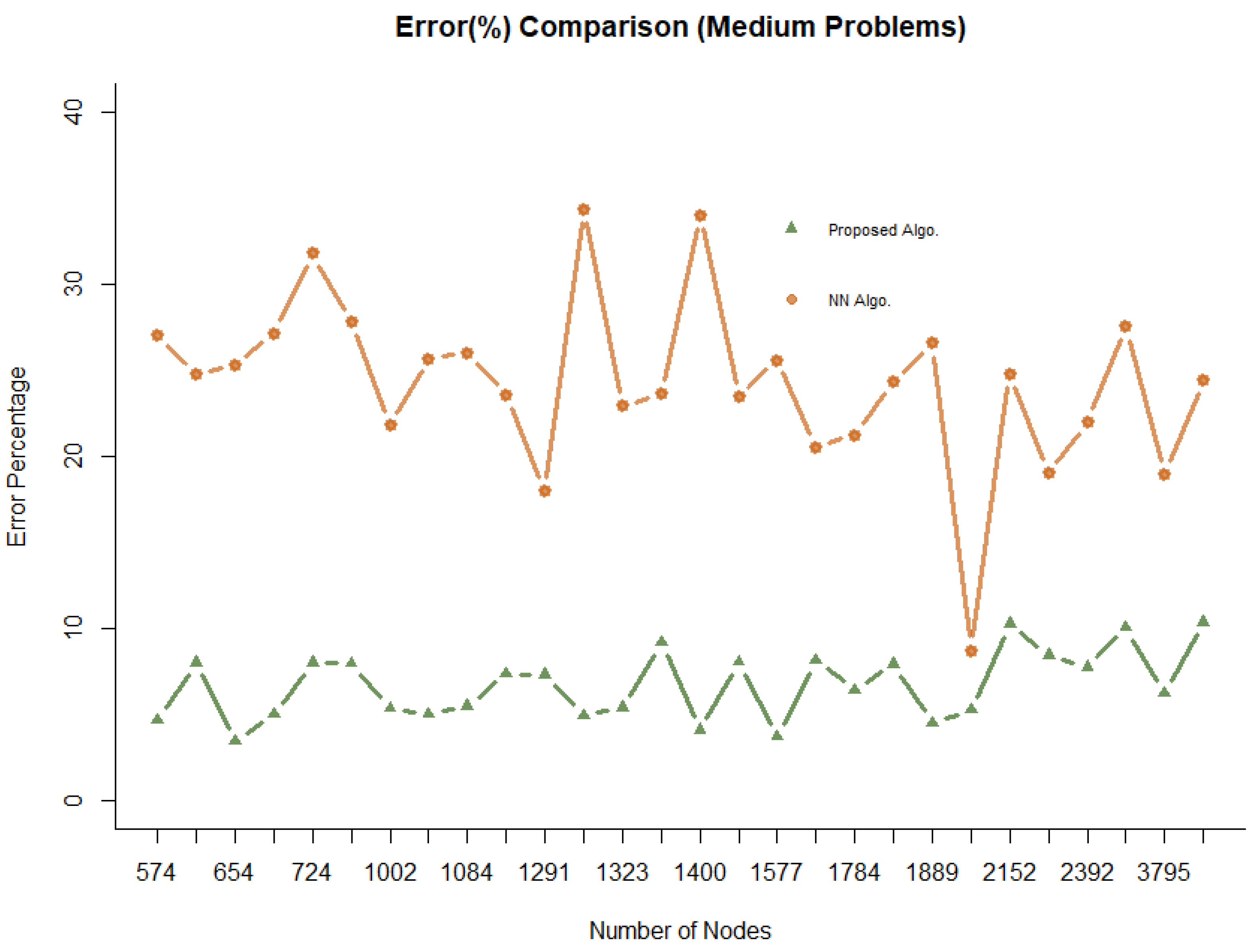
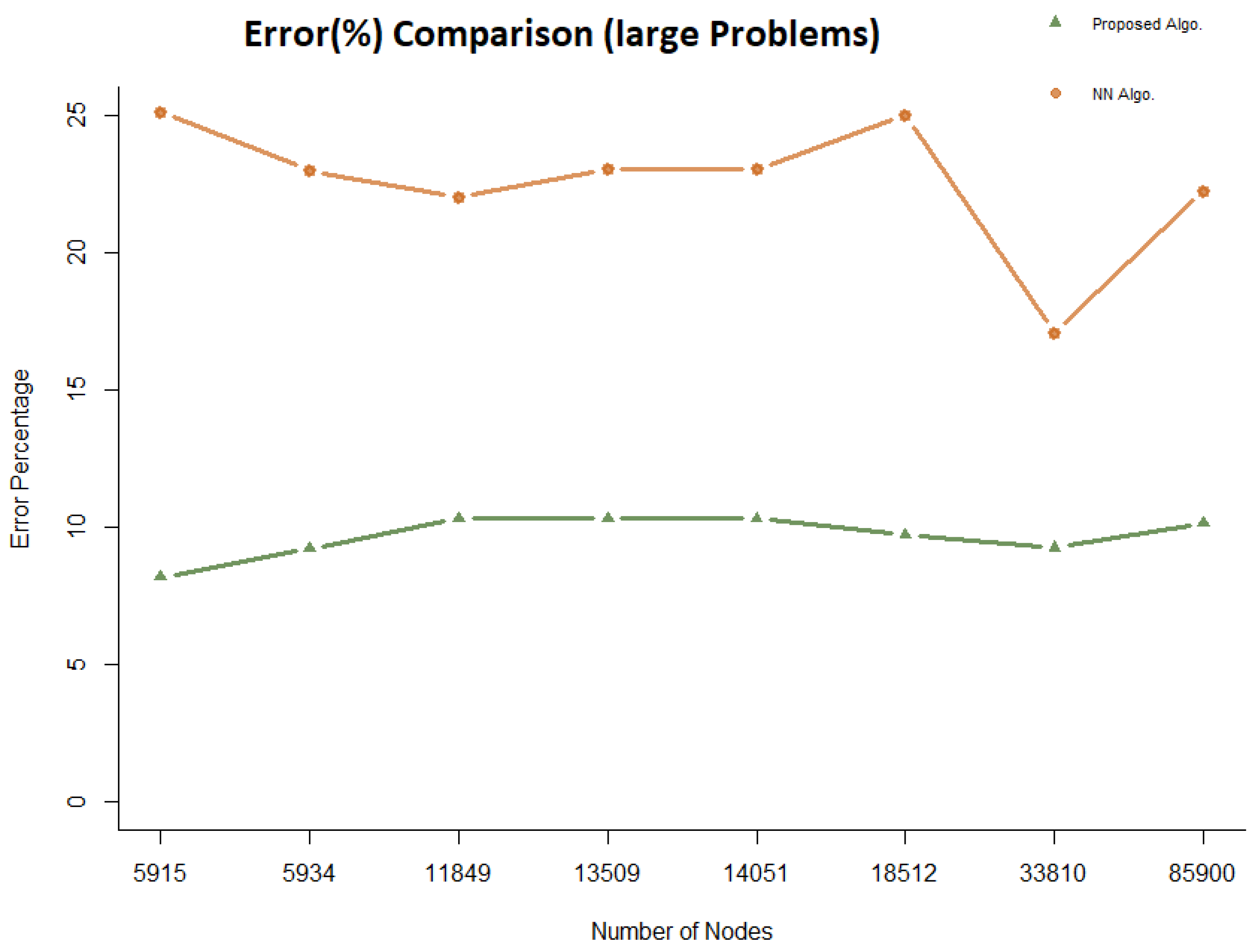
In this section, we present the results of the 2-Opt++ algorithm after deploying the graph compression technique for all three categories of problems: small, medium, and large. The results of small category problems are provided in Table 4, and the resultant comparison graph is depicted in Figure 7. For comparison’s sake, we also present the results of the nearest neighbour algorithm along with the results of the 2-Opt++ algorithm. An important point to be noted is that for all small category problems, our proposed algorithm produced an error margin percentage of below 7%. We would like to mention that only one of the problems, p264, produced a sub-par 13% error margin rate. However, once we added the number of active edges, it provided a much improved error rate of 3.78%. This means that all the problems were successfully managed under an error margin of 7%. In Figure 7, Figure 8 and Figure 9, we can clearly see that the variance of the error is lower in the 2-Opt++ algorithm as compared to nearest neighbour. We only considered NN for the comparison of larger problem instances (>1000 vertices) because, for the other algorithms, the resource and computation time requirements were simply huge. There are some techniques available to deal with larger problem instances in the literature, but they are implementation-dependent [27].

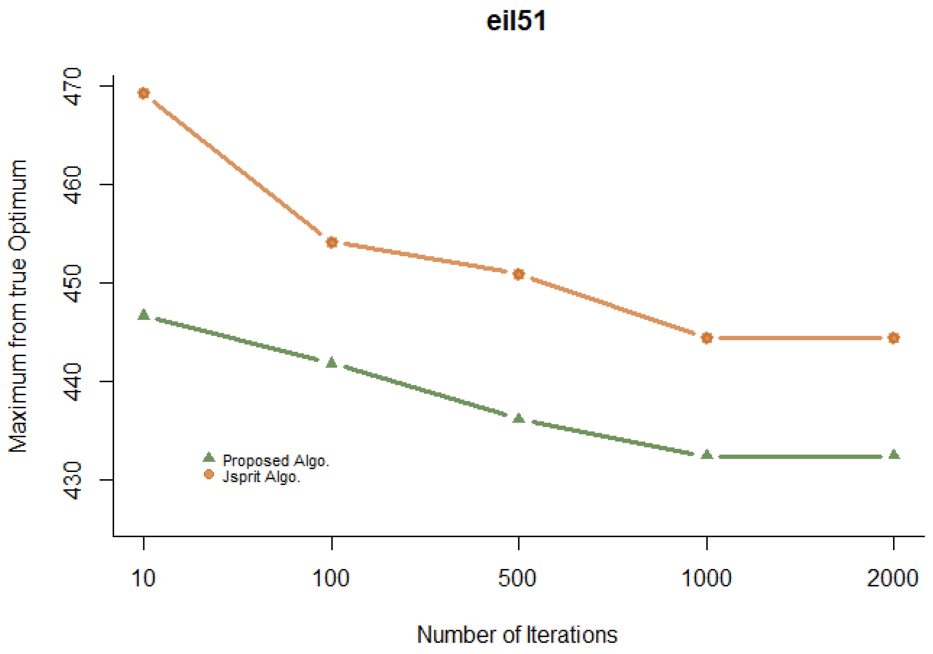
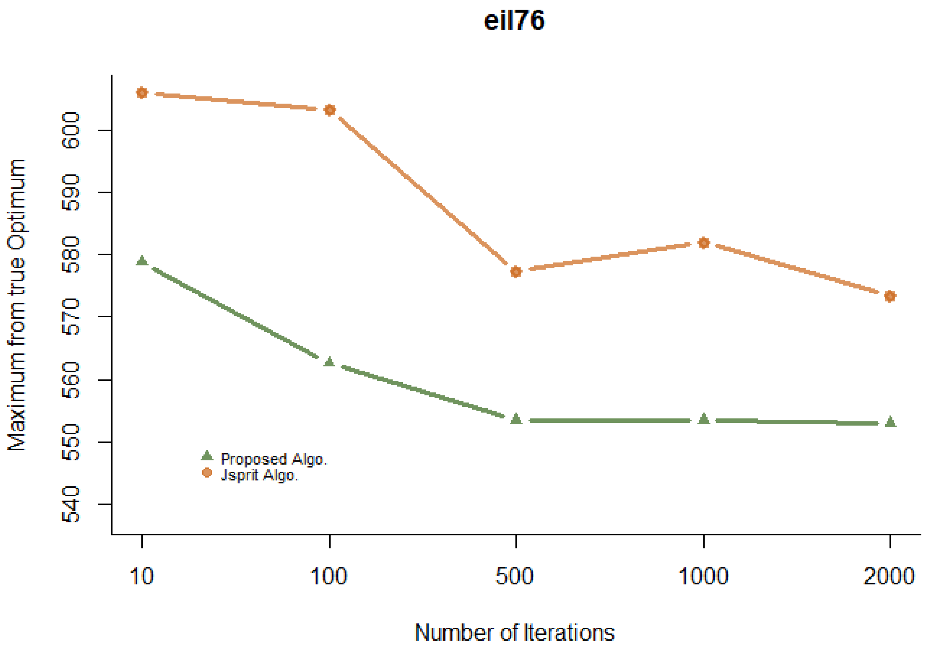
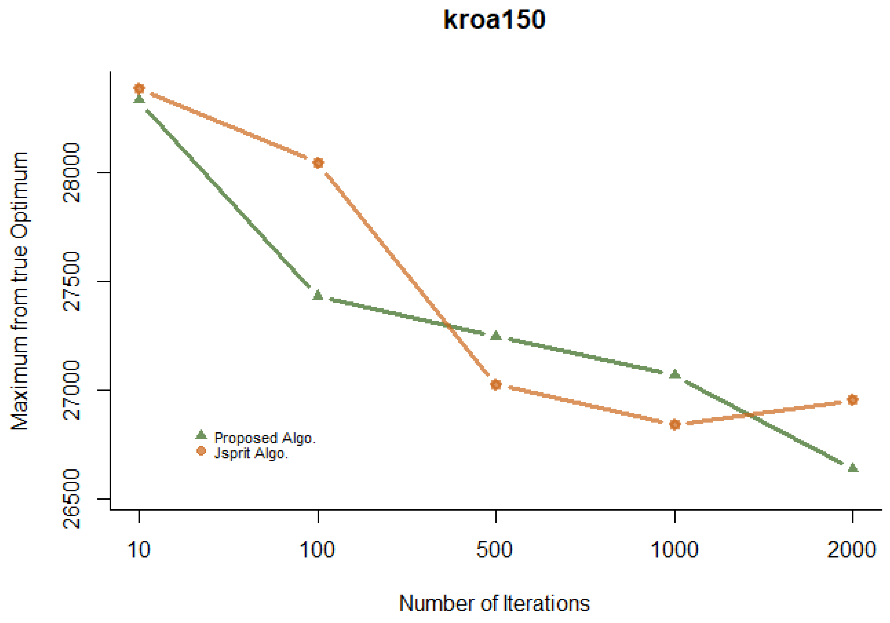
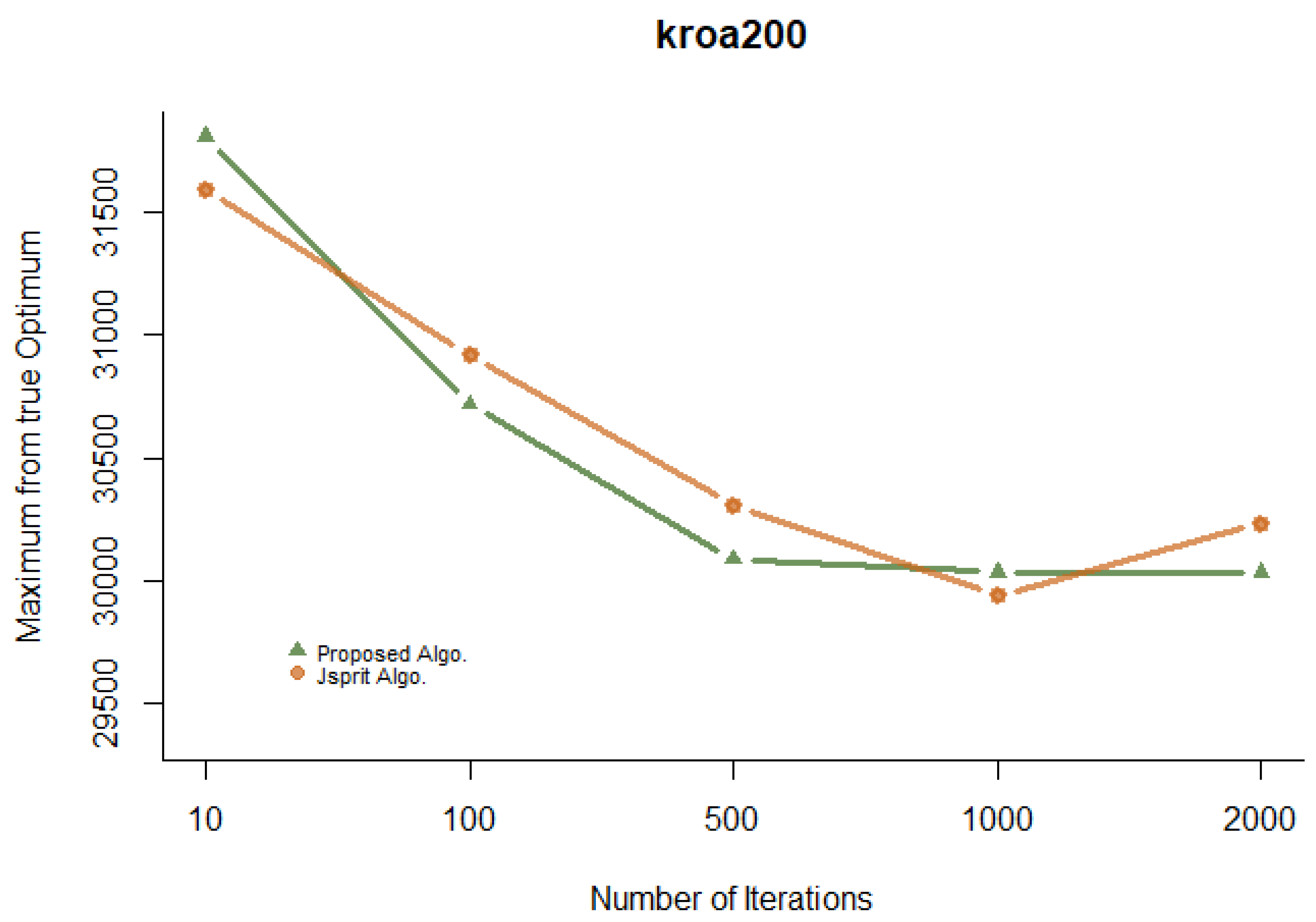
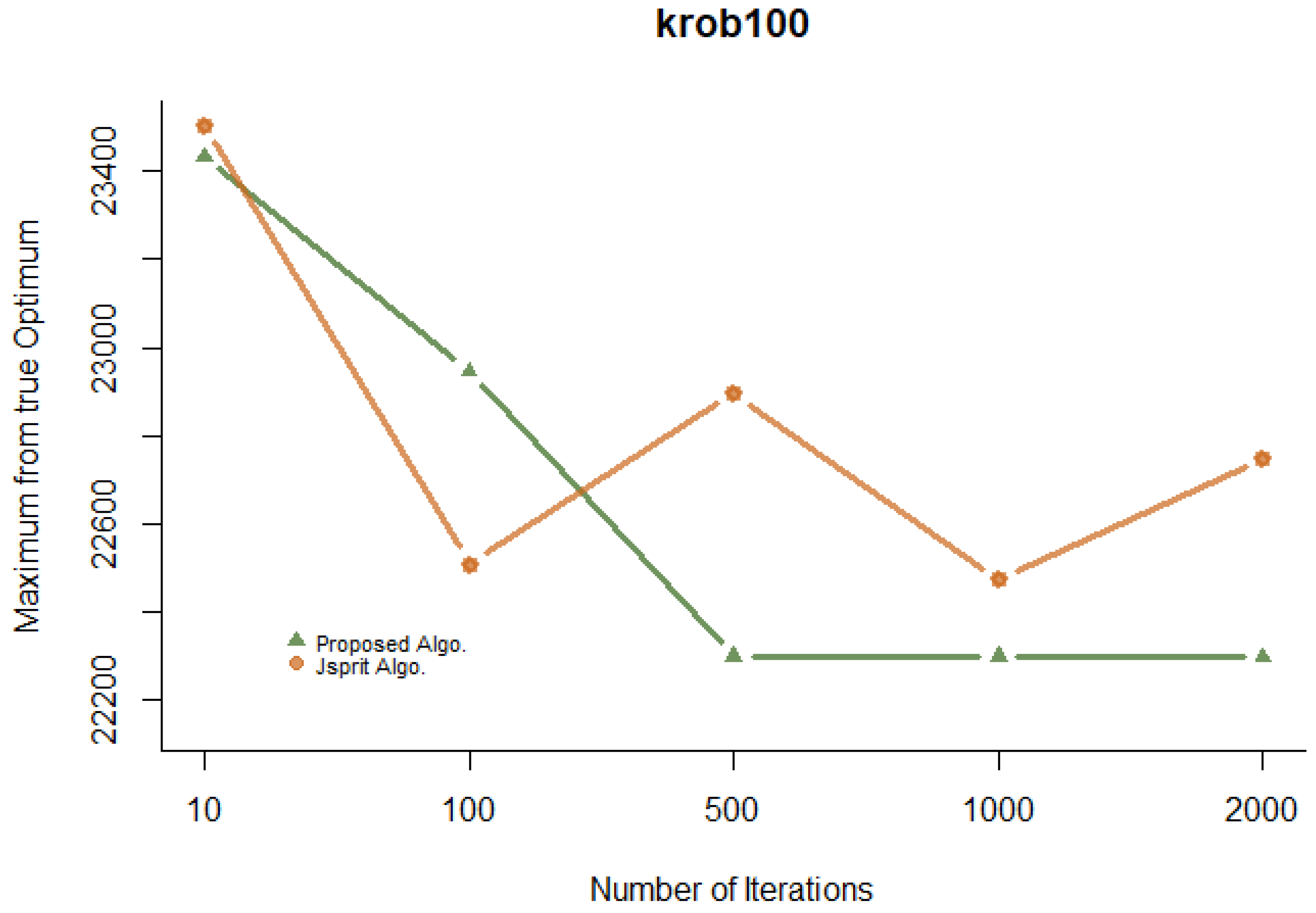
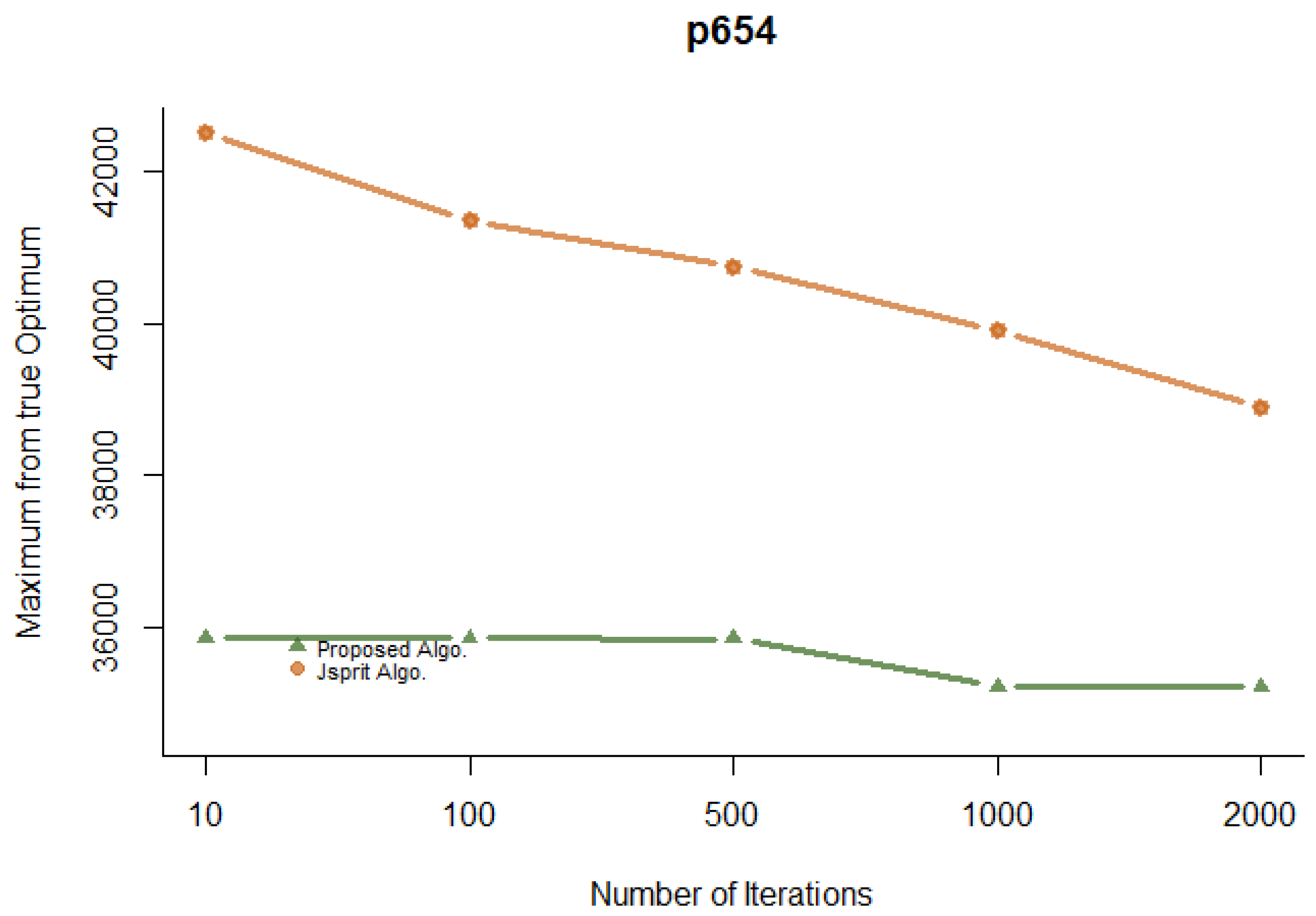
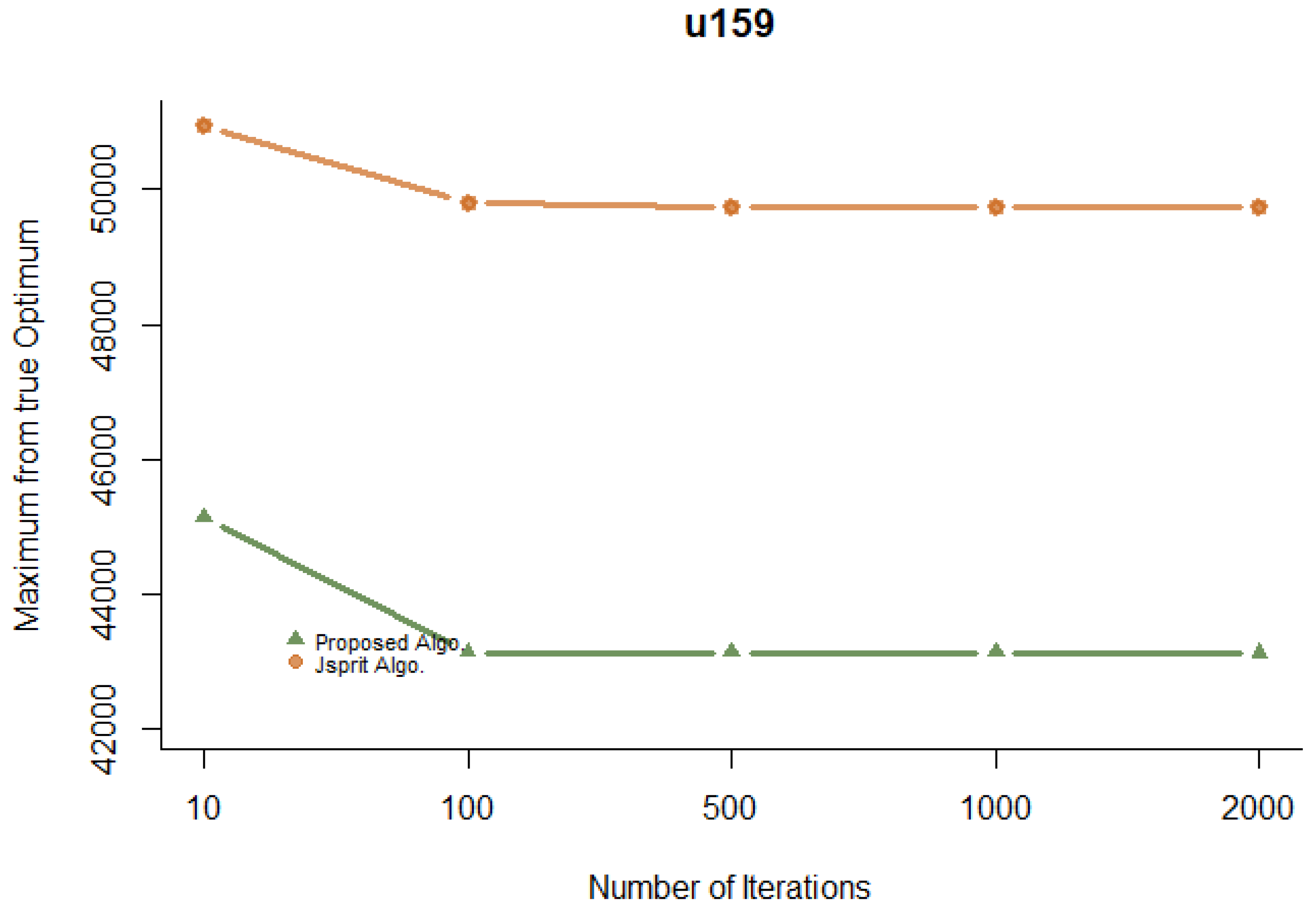
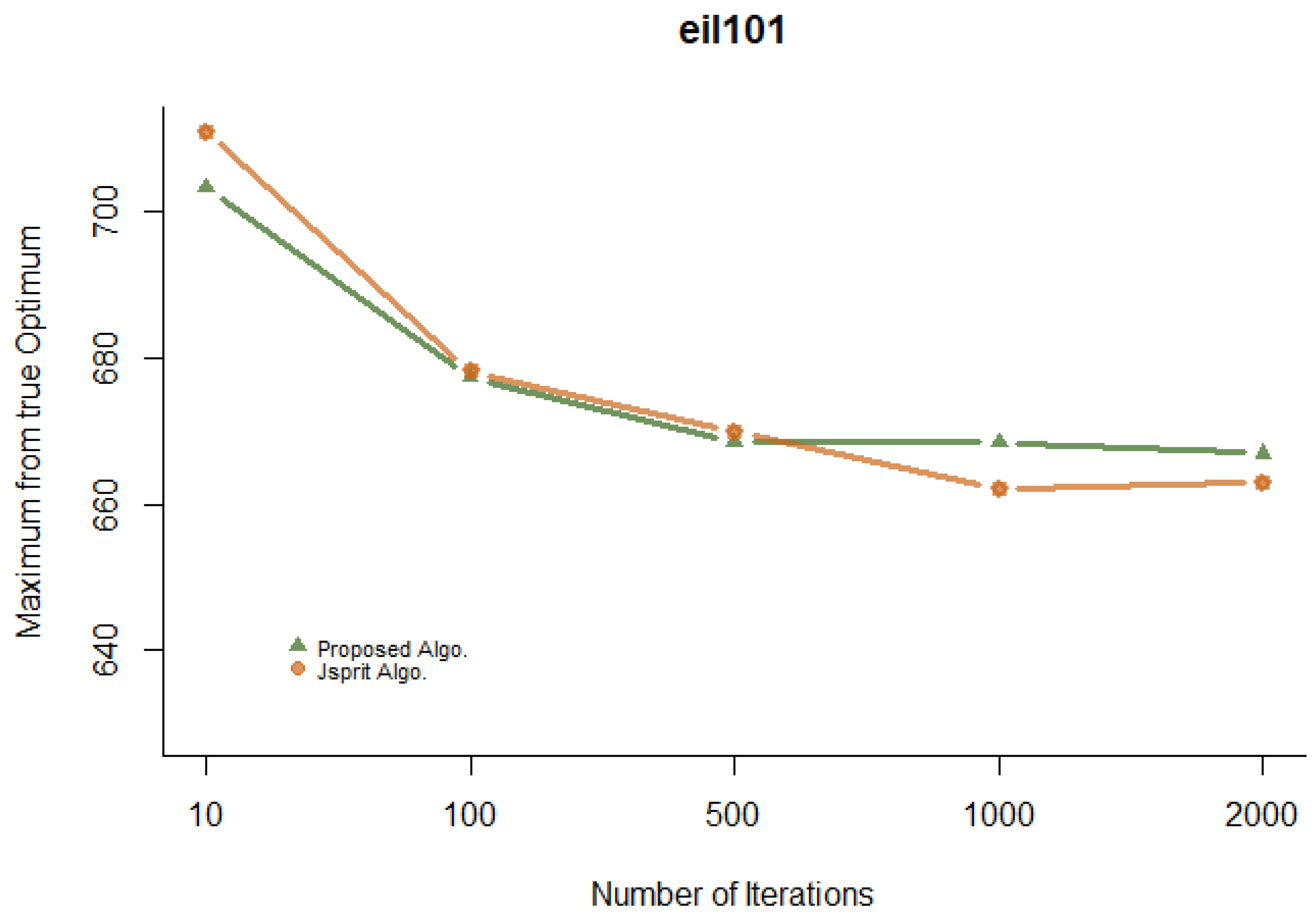
4.6. Convergence Analysis

In this section, we provide the graphs for the convergence of both the 2-Opt++ and $R\&R$ algorithms. For this purpose, we ran and executed the selected examples with 10, 100, 500, 1000, and 2000 iterations. We plotted the results for eight different problems Figure 10, Figure 11, Figure 12, Figure 13, Figure 14, Figure 15, Figure 16 and Figure 17. From the diagrams, it is clearly visible that, in general, the 2-Opt++ algorithm converged faster than $R\&R$. Only for one problem, i.e., eil101, although the 2-Opt++ algorithm performed well in the beginning, in the end, $R\&R$ showed better results in terms of convergence.

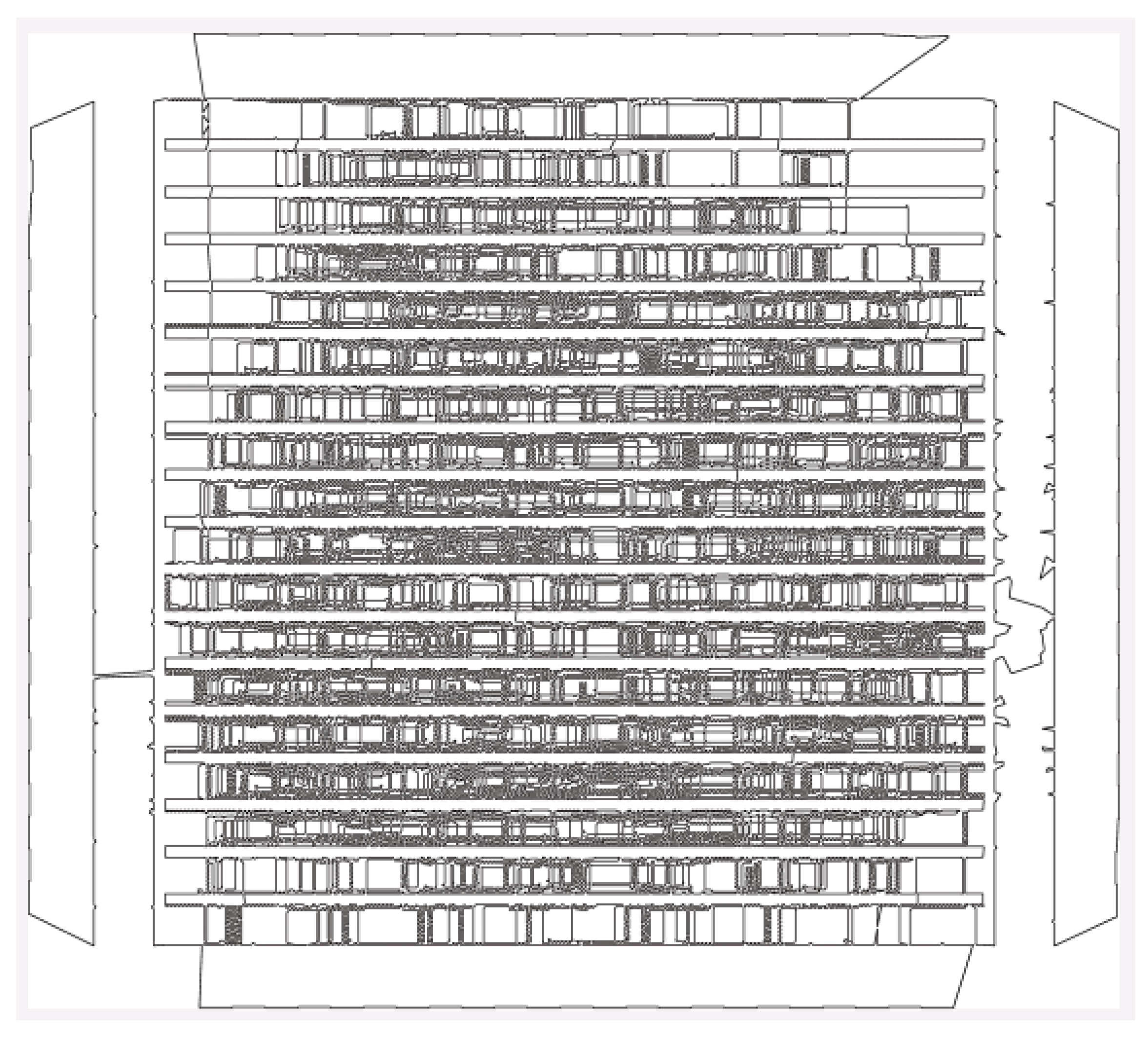
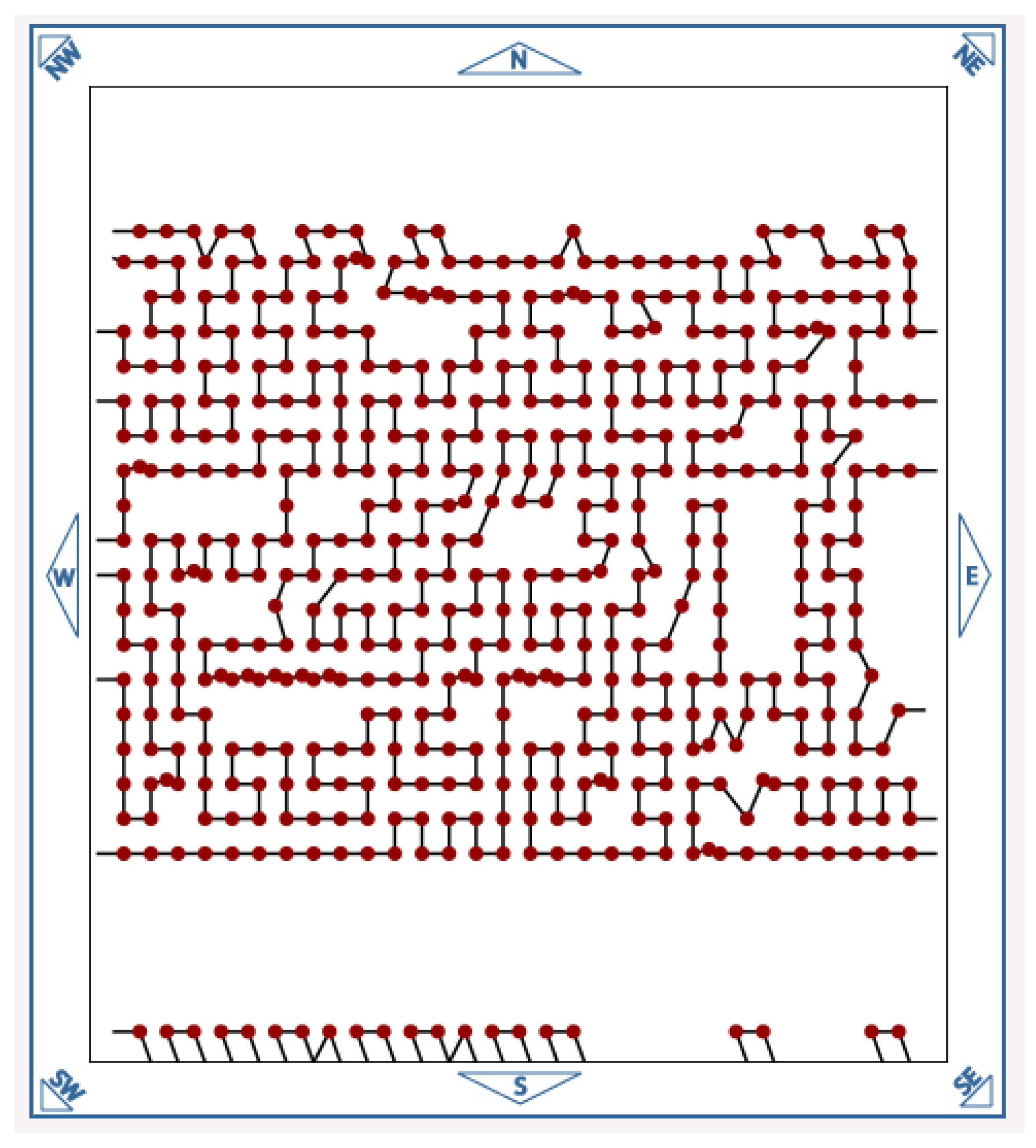
4.7. pla85,900 Solution

This is a special problem in the TSPLIB library. It consists of 85,900 nodes. It is the largest optimally solved problem for TSP. It was solved in 2005/06 with the Concorde algorithm [11]. Solving this problem with the 2-Opt++ methodology was a major challenge for us as it demanded huge memory resources. To represent this problem as a matrix, at least 55 GB of memory was required. The solution graph and a magnified view of this graph are shown in Figure 18 and Figure 19.

To address this huge memory requirement problem, we divided the large problem into four smaller problems. We solved these small problems and finally merged them to obtain the approximate solution. To break one large problem down into four small problems, we took the average of the x-axis points and y-axis points. All points on the x-axis that were less than the average value were placed below the virtual line, and all points on the x-axis that were greater than this value were placed over the line. This means that all the points that fell below the line were placed in the third and fourth quarters, while all points above the line were placed in the first and second quarters. The same technique was used with the y-axis points. Thus, we calculated all the points that fell within the first, second, third, and fourth quarters. We considered every problem as an independent problem and solved it; in the end, all problems were merged. This produced an error margin of 10.14%. In Table 4, the results of each small problem, the total best distance, and the computed error are provided.

5. Discussion

After analysing the results of 2-Opt++ with seven other algorithms in similar settings, we assert that the 2-Opt++ outperforms all other well-known algorithms in terms of (i) error variance; (ii) convergence; and (iii) computation time. In this section, we compare the average error and the average time taken by the 2-Opt++ and the R&R algorithm. For the 35 problems extracted from the TSPLIB library for the small category, the average error variance for $R\&R$ stood at 6.79%, while our 2-Opt++ produced 2.33%, which is a quite significant difference. Even for those cases where $R\&R$ produced a better result than our proposed algorithm, the difference was minor. The average time consumed by $R\&R$ and 2-Opt++ is 64.63 s and 2.41 s, respectively. These results show that our 2-Opt++ is efficient for almost all types of symmetric TSP problem instances.

We are also able to conclude that the NN algorithm is the fastest, followed by the 2-Opt++ algorithm, TPO, and GA. Based on the problem size, different algorithms show different patterns in time consumption. Tabu search and ACO depict exponential time increases as the problem size increases, while others show a slight increase in time with the problem size. In the average error comparison, 2-Opt++ performed outstandingly, followed by Tabu search, TPO, and GA. Tabu search’s better performance in terms of the average error could be due to its diversification mechanisms, such as swap, reversion, and insertion techniques, and the Tabu list, which ensures the best selection of the solution candidate. TS still shows up to a 64% error margin in a problem of 442 nodes. This problem can be addressed by using some other algorithms in the Tabu list mechanism. In terms of accuracy, GA shows consistent results, with error margins of less than 15% in all selected problems. It uses a mutation process, which drives it towards a better solution. If we compare the individual results, 2-Opt++ performs best, followed by TS, TPO, and GA.

6. Conclusions

The computational performance of 2-Opt++ is comparatively better than some other well-known techniques that provide approximate solutions to the symmetric TSP problem instances. The algorithm finds a tour with the minimum complexity and computational time using edge swap and graph compression/candidate list techniques, yielding an excellent solution in terms of the error margin. The graph compression technique/candidate list has been applied to solve relatively larger problems in a reasonable amount of time. In the first comparison, we compared and contrasted our results with the state-of-the-art algorithm known as ruin and recreate with respect to time, convergence, and error variance from the optimum results. In the second comparison, the results of the 2-Opt++ were compared with those of six other well-known algorithms published in a research paper [10]. The algorithms selected for the comparison were NN, GA, SA, TS, ACO, and TPO. The performance of our 2-Opt++ has proven to be impressive. We also considered the effect of using candidate lists in the third comparison.

In future work, we aim to employ multiple mutations for swap, reversion, and insertion and adopt better selection criteria, such as threshold acceptance or simulated annealing, over the existing greedy approaches to improve the results. A new and better technique can be devised for compression, which can take into account all the nearest points in 360 degrees. This will be of great importance in graphs where many points are assembled in a small area.