Article

Advanced Meteorological Hazard Defense Capability Assessment: Addressing Sample Imbalance with Deep Learning Approaches

1
Graduate School of Informatics, Osaka Metropolitan University, Osaka 559-8531, Japan
2
College of Computer and Information, Hohai University, Nanjing 211100, China
3
Research Institute, State Grid Jiangsu Electric Power Company Ltd., Nanjing 211100, China
*
Author to whom correspondence should be addressed.
Appl. Sci. 2023, 13(23), 12561; https://doi.org/10.3390/app132312561
Submission received: 9 October 2023 / Revised: 3 November 2023 / Accepted: 9 November 2023 / Published: 21 November 2023

Abstract

:
With the rise in meteorological disasters, improving evaluation strategies for disaster response agencies is critical. This shift from expert scoring to data-driven approaches is challenged by sample imbalance in the data, affecting accurate capability assessments. This study proposes a solution integrating adaptive focal loss into the cross-entropy loss function to address sample distribution imbalances, facilitating nuanced evaluations. A key aspect of this solution is the Encoder-Adaptive-Focal deep learning model coupled with a custom training algorithm, adept at handling the data complexities of meteorological disaster response agencies. The model proficiently extracts and optimizes capability features from time series data, directing the evaluative focus toward more complex samples, thus mitigating sample imbalance issues. Comparative analysis with existing methods like UAE-NaiveBayes, UAE-SVM, and UAE-RandomForest illustrates the superior performance of our model in ability evaluation, positioning it as a robust tool for dynamic capability evaluation. This work aims to enhance disaster management strategies, contributing to mitigating the impacts of meteorological disasters.

1. Introduction

As climatic volatility continues to escalate worldwide, the importance of preemptive evaluations in protecting communities from meteorological disasters has become increasingly paramount. These calamities, encompassing hurricanes, typhoons, tornadoes, and floods, not only unleash widespread destruction but also precipitate a harrowing loss of life and crippling economic setbacks. Hence, a meticulous assessment of disaster prevention mechanisms is vital, facilitating the fortification of areas like early warning systems that are crucial in curtailing damages. Through a nuanced appraisal of these mechanisms, authorities can channel resources judiciously, mitigating risks and fostering a state of readiness for potential emergencies. Consequently, the discerning evaluation of meteorological disaster prevention capabilities stands as a cornerstone in minimizing the adverse impacts of extreme weather phenomena on human life, assets, and the environment.
Historically, the proficiency of weather disaster response agencies has been gauged predominantly through expert rating methods. Despite their reliability, these methodologies are often marred by substantial time investments and financial burdens, consequently hampering the timeliness and efficacy of evaluations.
As we navigate these complex challenges, enhancing the emergency management capabilities of local governments emerges as a pivotal venture. A focus on the rigorous evaluation of government functionalities, encompassing their practices, efficacy, and efficiency, can potentially revolutionize the approach to emergency preparedness. By harnessing a scientifically robust assessment index system, governments stand to refine their operations significantly, slashing administrative overheads and amplifying overall effectiveness. This study, therefore, ventures into the realms of deep learning and data science, pioneering an innovative approach to tackle the intrinsic challenges of capability evaluations. Drawing upon the insights from recent studies such as Baihaqi (2023), it proposes adept solutions to counter the imbalances in sample data, setting a new standard for meteorological disaster defense evaluations [1].
Expertise in Emergency Management: Bryen D. N. (2009) posited that social organizations have inherent expertise in emergency management. They argued that governmental management agencies should oversee natural disaster emergency responses, emphasizing the need for comprehensive capabilities spanning pre-disaster preparedness to post-disaster recovery [2]. Corbacioglu Sitki et al. (2006) explored factors influencing emergency response capabilities, encompassing technology, information, cooperative communication, and cultural development [3]. Adding to this discourse, Mah Hashim et al. (2023) highlighted the necessity for a coordinated system to manage flood disasters in Malaysia, suggesting a more efficient framework for flood governance [4].
Integration of Performance Monitoring Methods: Kathy Zantal-Wiener et al. (2010) suggested incorporating performance monitoring methods from the U.S. education sector into the Government Performance and Results Approach (GPRA) to enable holistic evaluations [5]. Meanwhile, JinFeng Wang et al. (2012) employed a wavelet neural network in assessing coal mine inundation disaster response capacities [6]. Sugumaran et al. (2017) proposed a model to assess emergency organization capabilities, offering insights for varying local emergency management entities [7]. In a similar vein, Kyrkou et al. (2023) con-ducted a comprehensive survey on the application of machine learning algorithms in emergency management, identifying promising avenues for leveraging these technologies in various phases of disaster management [8].
Academic Interest in Natural Disasters: The academic sphere has long been intrigued by natural disasters, with a recent surge in interest around the theoretical exploration of crisis management due to societal shifts caused by human rights movements, ideological changes, and economic crises. Scholars have delved into government decision-making and implementation mechanisms, striving to ensure the scientific soundness of policies addressing natural disasters. Over time, the theories around natural disaster management have matured and diversified in research directions, a trend echoed in the works of Herlianto (2023), who emphasized the importance of early disaster recovery strategies in post-disaster implementation in Indonesia [9].
Legal Frameworks and Policies: The study of the formulation of laws, establishment of management systems, and preparation of emergency plans for natural disaster management has been the focal point of many academics, aimed at bolstering governmental emergency management capabilities. The U.S., starting in the 1980s, progressively introduced legislative frameworks such as the Flood Control Act and the Natural Disaster Mitigation Act to govern the emergency management of natural catastrophes [10]. The Disaster Relief and Emergency Assistance Act of 1974 established a foundation for the U.S. federal government to support state and local governments, delineating guidelines for post-disaster relief and rescue operations. Meanwhile, Japan’s Disaster Relief Act integrated the concepts of disaster mitigation and prevention into a singular legislative framework. This was succeeded by the Basic Law for Disaster Countermeasures, transitioning Japan’s legal framework from a singular response system to a multi-faceted comprehensive system. This shift emphasized institutional structuring, early disaster warnings, plan development, emergency response, and post-disaster recovery and rebuilding [11]. Furthermore, the Basic Countermeasures for Natural Disasters Act laid the foundation for Japan’s preventative and mitigation strategies [12].
Innovative Studies and Technological Advancements: Recent studies have ventured deeper into the nuances of management strategies and institutional evolution. Junfeng Yao et al. (2023) utilized network analysis and the Petri net model to foster organizational collaboration, concentrating on the synergy of emergency management entities and disaster response protocols, thereby enhancing efficiency and reducing response time [13]. On another front, Ling Shen et al. (2023) leveraged a social networking perspective to amplify emergency management competencies, advocating for a collaborative governance mechanism involving multiple entities, particularly emphasizing grassroots governments [14].
In the era of big data, Zhenling Liu and Liang Ma (2022) navigated the complexities of governmental emergency responses, pinpointing the transformative role of digital government in reshaping government management and business structures and suggesting institutional reforms to harness new opportunities in democratic politics [15]. Similarly, C. J. Wang et al. (2020) critically evaluated Taiwan’s emergency response mechanisms during the COVID-19 pandemic, proposing avenues for improvement using big data analytics and new technology for proactive testing, thereby safeguarding public health through timely and transparent information dissemination [16]. The recent advancements in information technology have facilitated the standardization and automation of primary behavioral data for meteorological disaster agencies [17]. Consequently, capability evaluations have increasingly incorporated data-driven methodologies, such as machine learning and deep learning, yielding promising results. Nonetheless, integrating deep learning techniques into the assessment of emergency response capacities for weather-related disasters has unveiled certain mismatches and issues [18]. This arises primarily because machine and deep learning algorithms adjust model parameters based on the loss function values of training data, making the loss function a foundational element for model training regarding capacity evaluation rules.
The existing loss functions, however, have shown some limitations in assessing weather hazard response capabilities:
(1)
The capability spectrum across weather disaster emergency response agencies is diverse, and current loss functions tend to undervalue agencies with lower capabilities. For instance, out of the capability evaluation results for 1249 agencies released by the National Meteorological Administration in 2017, only 121 agencies scored below grade A. This indicates an unbalanced distribution of capability levels. With the current loss function, during the training of deep learning models, a handful of low-grade agencies might be misclassified as high-grade ones. Drawing from 2017 data, even if all 1370 agencies were ranked AA or above, the cumulative loss would merely be 8.8%.
(2)
Due to factors like inconsistent attention, variance in evaluation difficulty for institutional meteorological disaster response capabilities, and the present loss function, it becomes arduous to focus the evaluation model on entities that pose evaluative challenges. The essence of a capability evaluation is to spotlight agencies that demonstrate subpar capabilities, enabling the deployment of specific, tailored supervision [19]. However, evaluation bodies don’t uniformly allocate attention to their assessment outcomes. While the capability evaluation model can more easily discern capability levels from metrics like institution size and qualifications, for a minority of entities, ascertaining their capability levels via competency attributes is tough. Furthermore, agencies, especially those with diminished capabilities or those that are hard to evaluate, draw significant attention from actual management. The standard loss function used in contemporary machine learning models for capability evaluation struggles to adapt to imbalanced data. It disproportionately emphasizes easy-to-identify samples over complex ones, undermining the model’s generalization performance [20].
Addressing the challenges of overlooking hard-to-rate agencies and accurately distinguishing low-capacity disaster defense entities in current capacity evaluation models requires a nuanced approach [21]. Enhancing the deep learning algorithm from the perspective of the loss function offers a promising avenue. The modified loss function, during the training of the deep-learning-based capability evaluation model, can be tuned to spotlight disaster defense agencies that are inherently complex to categorize [22]. By doing this, the penalty for inaccurately classifying low-rated and challenging-to-rate agencies is augmented. Here’s an in-depth look at the steps proposed:
(1)
Weighted Loss Function Addition: By embedding a weighted loss function, the model is oriented toward paying extra attention to specific low-capacity-rank agencies. Given the uneven capability distribution among weather disaster emergency response agencies, the traditional loss function can be appropriately weighted [23]. By doing so, the loss function value for sparse low-capacity samples is augmented, leading to higher penalties for misclassifications. Consequently, the inherent losses from poor assessments of low-capacity agencies are curtailed [24].
(2)
Adaptive Focal Loss Function Integration: To focus on meteorological disaster response agencies with ambiguous capability levels, an adaptive focal loss function is established. This function, crafted around the classification error trends exhibited by agencies during model training, instructs the evaluation model to zero in on those agencies that present significant evaluative challenges. Theoretically, the focal loss function rectifies the imbalance between high and low capability samples throughout training, potentially outperforming preceding methods. The idea is that this scaling factor will automatically decrease the weight of straightforward samples during training, spotlighting those tricky-to-identify low-capacity entities.
(3)
Comprehensive WAFL Loss Construction: Combining the previously discussed loss functions, a holistic WAFL (Weighted Adaptive Focal Loss) function is proposed. This function, which contemplates both potential misclassification scenarios mentioned above, offers a harmonized blend of both. From an analytical perspective, merging weighted and focal losses enhances the prevailing model both at the sample level and during the training phase. This synthesis proves to be particularly beneficial for gauging the capability of entities in the water resources sector and appraising the risks linked with engineering quality.
(4)
WAFL-Based Deep Learning Algorithm Examination: With the WAFL loss function as a foundation, this delves into the intricacies of the deep neural network’s forward computation, error propagation, and parameter updating mechanisms. By harnessing the capabilities of the WAFL-based deep learning algorithm, a robust capability evaluation model can be crafted.
By following the above blueprint, the groundwork for constructing competency evaluation models has been laid. After this, the focus can be directed toward interpreting evaluation outcomes and contrasting the results of diverse models using empirical datasets. This systematic approach ensures a more holistic and accurate capability evaluation of agencies, addressing the inherent challenges presented by the current models.

2. Materials and Methods

In recent times, machine learning algorithms, including support vector machines and deep learning, have become prominent in capability evaluation problems [25]. Typically, machine learning models employ the loss function as the optimization objective for training model parameters [26,27]. For capability evaluation, the cross-entropy loss function is predominantly used, as represented in (1).
L C E p i , y i = y i T log p i
In this Equation, y i represents the actual ability level of the ith sample, and p i represents the predicted probability distribution generated by the competency evaluation model for the competency level of the ith sample.
Before we delve into the details of the Weighted Adaptive Focus Loss (WAFL) function, it is essential to define the terms “simple”, “difficult”, and “anomalous” samples.
Definition 1.
Suppose that the capability characteristics of the ith sample are denoted by xi, and the true value of the capability level is represented by yi. The capability levels of the construction weather disaster emergency agency are categorized into five levels: AAA (very good capability), AA (good capability), A (better capability), BBB (average capability), and CCC (poor capability), respectively.
yi belongs to the set {AAA, AA, A, BBB, CCC}. For each yi, a One-Hot encoding method is used, utilizing a 5-bit status register to represent the 5 ability levels. Each level has its own independent register bit, and only one bit is valid at any given moment. The representation in One-Hot encoding is as follows:
y i [ 1,0 , 0,0 , 0 ] T , [ 0,1 , 0,0 , 0 ] T , [ 0,0 , 1,0 , 0 ] T , [ 0,0 , 0,1 , 0 ] T , [ 0,0 , 0,0 , 1 ] T
The predicted probability distribution of the ability levels is denoted by p i , given by:
p i = P y i = 1,0 , 0,0 , 0 T , P y i = [ 0,1 , 0,0 , 0 ] T , P y i = [ 0,0 , 1,0 , 0 ] T , P ( y i = [ 0,0 , 0,1 , 0 ] T ) , P ( y i = [ 0,0 , 0,0 , 1 ] T ) T .
Assuming that the capability characteristics of the first sample are denoted by xi, the true value of the capability level is denoted by yi, and the predicted value of the capability level is denoted by pi, we define the following types of samples:
(1)
Simple sample: a sample whose ability level can be easily discerned by the model, i.e., the sample whose predicted label value closely matches the true value. The closer the error | y i p i | is to zero, the simpler the sample is.
(2)
Difficult samples: samples for which the model finds it hard to correctly determine the ability level, i.e., samples with predicted label values significantly differing from the true values. The larger the error | y i p i | , the more challenging the sample is.
(3)
Anomalous samples: extreme cases within the difficult samples, deviating significantly from the normal distribution, such that not even the optimal model can classify them correctly.
The sample types are defined in Definition 1 based on the error in determining the ability levels. As illustrated, difficult samples vary significantly from both simple and abnormal samples. The existing loss function of the model is not tailored to address this subset of samples, resulting in a substantial classification error for them. If the loss function, as depicted in Equation (1), leads to a total loss dominated by a majority of high-ability-level samples, the ability evaluation model may find it challenging to distinguish between samples with lower ability levels. To address this, enhancing the loss function coupled with specific sampling techniques can facilitate the generation of simple samples from difficult ones, highlighting that difficult samples are not synonymous with abnormal samples.

2.1. Loss Function Construction

2.1.1. Category-Weighted Loss Function

Data imbalances across different ability levels are a prevalent issue in data evaluations. To address this, researchers commonly employ data sampling methods and loss function optimization techniques. This paper introduces category weights αi to enhance the conventional cross-entropy loss function, aiming to mitigate the imbalance problem in sample categories.
Definition 2.
Let S{(xi, y)j |i = 1, 2, …N} be the set of training samples created by the ability evaluation model.  y i  indicates the category of the ith sample,  N y i  represents the count of samples in the same category as yj, and  N y i  represents the count of samples in categories other than yj, and  N y i + N y i = N , thus
α i = N y i N y i + N y i , α i 0,1
Here, αi denotes the weight of the ith sample. The magnitude of αi in Definition 2 positively correlates with N y i and negatively correlates with N y i , meaning that if the sample (xi, yj) falls into the majority category, its loss weight is reduced. Therefore, incorporating category weights αi into the cross-entropy loss function can augment the impact of a minority of low-ability-level samples on the loss function and diminish the loss weights of high-ability-level samples, thus neutralizing the loss discrepancies induced by the imbalanced distribution of high- and low-ability-level samples.
Definition 3.
Given yj and pj as illustrated in Definition 1, we have
L α p i , y i = α i y i T log p i
This Equation represents the category-weighted cross-entropy loss function. The distinction between Equation (3) and the standard cross-entropy loss function is the inclusion of sample category weights αi to counterbalance the loss variation arising from differing sample counts across categories. If αi is designated as 1, then Equation (3) reverts to the standard cross-entropy loss function.

2.1.2. Adaptive Focus Loss Function Construction

To address the disproportionate ratio of simple to difficult samples, Yang Lian and others introduced a cross-entropy function grounded on Focal Loss (FL). This concept posits that the abundance of simple samples in the dataset, which predominantly govern the total loss, have a negligible influence on model refinement. Therefore, the model should prioritize difficult samples. Accordingly, a focus parameter γ γ 0 is integrated into the loss function to lessen the contribution of simple samples to the total loss.
Definition 4.
With yj and pj defined as in Definition 1, we state that
L F o c a l p i , y i = | y i p i | γ y i T log p i
This Equation embodies the focal loss function. As inferred from Equations (3) and (4), the simpler the sample, the closer p i is to y i , and the smaller | y i p i | γ , hence the factor | y i p i | γ serves to diminish the contribution of simple samples while amplifying that of difficult samples. The larger the γ value, the more pronounced this effect becomes [28].
However, considering that meteorological disaster emergency response capability assessments are conducted by experts, a degree of subjectivity is unavoidable. This leads to partial evaluations of the capability profiles of disaster response agencies and the occurrence of mislabeled samples. In this study, these mislabeled samples are termed anomalous samples. Although anomalous samples are not classified as difficult samples, emphasizing them excessively during training can hinder the model from learning the true data distribution efficiently. This not only squanders computational resources and prolongs training time, but also escalates the likelihood of overfitting, showcasing the limitations of Focal Loss. Consequently, this paper proposes an adaptive focal loss function to overcome these issues.
Definition 5.
Let yj, pj be as defined in Definition 1. Then, the adaptive focal loss function is given by
L A d a p t i v e F o c a l p i , y i = s i y i T log p i
where
s i ( e ) = ρ s i ( e 1 ) + ( 1 ρ ) d i f f i e 1
d i f f i ( e 1 ) = | | y i p i | ( e 1 ) | y i p i | ( e 2 ) |
Here,  e  represents the number of training rounds.  d i f f i ( e 1 )  denotes the difference in training error between the  e 1  th round and the previous round for sample  i , with  d i f f i ( 0 ) = 0 .
From Definition 5, we observe that s i ( e ) represents the accumulated value of d i f f i for sample i up to the e 1 th training round, indicating the degree of difficulty in classifying that sample. When e = 1 , s i ( 0 ) = 1 . The hyperparameter ρ , ranging between [0,1], controls the adjustment magnitude of d i f f i ( e 1 ) on s i ( e ) . The smaller the value of ρ , the greater the correction effect exerted by d i f f i ( e 1 ) on s i ( e ) . It is evident that L Adaptive - Focal   p i , y i at the eighth round is influenced by the accumulated error differences from all previous rounds. If ρ = 1 , then d i f f i ( e 1 ) will not impact s i ( e ) , making s i perpetually equal to 1, which reduces L Adaptive - Focal   p i , y i to L C E p i , y i . Conversely, if ρ = 0 and d i f f i ( e 1 ) remains constantly equal to y i p i ( e 1 ) , then L Adaptive - Focal   p i , y i simplifies to L Focal   p i , y i .
As the model undergoes more training rounds, d i f f i ( e 1 ) varies continually. If d i f f i ( e ) stays relatively small over several rounds, it signifies a lack of significant improvement in the model’s fit to sample i during those rounds. This can occur due to two reasons:
(1)
The loss associated with sample i has nearly minimized as the training rounds have increased.
(2)
Sample i is anomalous, and the model is unable to learn the correct distribution. In both scenarios, the value of s i will decrease, thereby reducing the loss value L Adaptive - Focal   p i , y i , fulfilling the goal of minimizing the loss for simple and anomalous samples.

2.1.3. Weighted Adaptive Focus Loss Function

To address the issues of category imbalance and uneven classification difficulty encountered in ability evaluation, this paper proposes the integration of category weights and the newly developed adaptive focal loss to enhance the cross-entropy loss function. This enhancement aims to bolster the ability evaluation model’s proficiency in identifying samples characterized by low ability levels and greater classification challenges.
Definition 6.
Let  y j , p j  be as defined in Definition 1 and let  α i , s j  be as defined in Definitions 2 and 5. Then, the weighted adaptive focus loss function is expressed as
L α A d a p t i v e F o c a l p i , y i = α i s i y i T log p i = α i s i L C E p i , y i
This loss function, outlined in Definition 6, amalgamates the category weights α i of the samples and the classification difficulty s i . Consequently, the training of the parameters in the ability evaluation model can be more acutely fine-tuned toward the samples with low ability levels that are not readily categorized. The values for α i and s i can be deduced from Equations (2) and (6), respectively.

2.2. Deep Learning Model for Evaluating Weather Disaster Emergency Response Capacity

A deep neural network, a type of multilayer feedforward neural network, operates based on the error backpropagation algorithm. Due to its profound nonlinear representation capability, many researchers have utilized it for capability evaluation in recent years, yielding commendable results [24,29]. In this study, we integrate the newly constructed weighted adaptive focal loss function with the deep neural network. This combination aims to refine the weather disaster emergency capability evaluation model, placing greater emphasis on the loss weight for sparse low-capability-level samples and challenging samples. This enhancement optimizes the model’s ability to recognize pivotal samples. The model construction, akin to other deep learning models, encompasses three primary phases: forward propagation of capability information, backward propagation of the error gradient, and updating of network parameters based on the gradient [30].

2.2.1. Forward Calculation

The weighted adaptive focus loss function formulated in this paper is depicted in Equation (8). As a function reliant on the output value of the ability evaluation model, it necessitates the application of the neural network’s forward propagation to ascertain the loss function’s value. The forward propagation of ability information entails the input of the institution a i ’s ability feature data into the model. Through the utilization of each hidden layer’s linear mapping matrix and non-linear activation function, a successive feature mapping is performed, culminating in the prediction of the institution’s ability level at the output layer. The loss function calculation doesn’t impinge on the deep learning forward propagation process; hence, this paper’s model forward calculation aligns with that of the deep neural network model.
Suppose the model comprises ‘Layers’ network layers, where C l , W l , and b l , and g l , z l , and r l represent the number of neurons, the weight matrix, and the bias vector in the l th   layer, as well as the activation function, the input to the activation function, and the output at the l t h layer (with l ranging from 1 to M ), respectively. The attributes such as capability characteristics, the true capability level, and the predicted capability level of the i th   weather disaster emergency agency in area i are represented by a i , y i , and p i , respectively, where i falls within the range of { 1,2 , , N } .
The forward propagation operates under the following principles:
(1)
a i serves as the input to the deep neural network. The first layer’s activation function input, z 1 , i , is determined through the first hidden layer as elucidated in Equation (9):
z 1 , i = W 1 a i + b l
(2)
z 1 , i is activated, undergoing a non-linear transformation as delineated in Equation (10):
r 1 , i = g 1 ( z 1 , i )
(3)
Following calculations at the M 1 layer, the output r M 1 , i corresponding to a i is acquired. The predicted value p i is then computed as
z M , i = W M r M 1 , i + b 2
p i = g M ( z M , i )
Ability evaluation constitutes a multi-classification issue, typically utilizing the Softmax function as the output layer’s activation function g M . This is represented as
p i = e z M i j = 1 n l M e z j
where z M i denotes the M th   hidden layer’s output value for the i th   sample, and n l M indicates the number of nodes at the M th   layer.

2.2.2. Error Backpropagation

Contemporary deep learning models for capability evaluation often utilize the cross entropy defined in Equation (1) as the loss function to juxtapose the forecasted values, derived during the forward propagation, with the true values. This approach helps calculate the gradient values of the network parameters and disseminates them in a backward fashion. Contrastingly, this study employs the Equation (8) L α - Adaptive - Focal   p i , y i as the model’s loss function.
Consequently, both the gradient calculation and the backward propagation processes of the model parameters diverge from those seen in conventional deep learning models.
Given that the problem at hand is multiclassification, y i is represented as a One-Hot vector, with L α - Adaptive - Focal   p i , y i designating the loss value. Assuming a deep neural network model comprising ‘Layers’ layers, we aim to calculate the gradient of the model parameters at layer l . Here, g l z l symbolizes the derivative of the output r l from the l th layer’s hidden node z l within deep learning layer l , and the partial derivative of L α - Adaptive - Focal   p i , y i with respect to z l , denoted as δ l , can be defined as
δ l = L α   Adaptive - Focal   p i , y i z l = α i s i L C E p i , y i z l
This Equation further transforms as
= α i s i L C E p i , y i z l + 1 z l + 1 r l r l z l = α i s i W l + 1 T δ l + 1 g l z l
According to Equation (14), the gradient value of any layer’s parameter is a function of the preceding layer. Given that there are no neurons following the final layer of ‘Layers’, its δ value is
δ Layers   = L α   Adaptive - Focal   p i , y i z Layers   = α i s i L C E p i , y i z Layers   = α i s i p i y i
where l { 1,2 , , Layers -1 } , and, using Equations (14) and (15), the partial derivatives of L α - Adaptive - Focal   p i , y i with respect to z at each layer can be recursively computed in reverse. Subsequently, according to the chain rule, we can pinpoint the partial derivatives of L α - Adaptive - Focal   p i , y i concerning the weight matrix W l of the l th layer,
L α - Adaptive - Focal   p i , y i W l = L α - Adaptive - Focal   p i , y i z l z l W l = α i s i L C E p i , y i z l z 6 W l
Here, α i can be procured from Equation (2), and s i can be inferred from Equations (6) and (7). Moreover, δ l can be inferred from Equations (14) and (15), and r l 1 can be deduced from Equations (9)–(11).

2.2.3. Network Parameter Update

As per Equation (16), we obtain the Jacobian matrix of the partial derivatives for the weight matrix of each layer by calculating the loss function. Utilizing this matrix, we can ascertain the necessary adjustments to W l to accordingly alter L α - Adaptive - Focal   p i , y i . The objective of model training is to steadily decrease the loss value until reaching the global optimum. In this pursuit, we modify W l in Equation L α   Adaptive - Focal   p i , y i W l in the direction opposite to the gradient to minimize L α - Adaptive - Focal   p i , y i . This method is termed Gradient Descent (GD).
The formula is given by
W l = W l l r · L α A d a p t i v e F o c a l p i , y i W l = W l l r · α i s i δ l r l 1 T
In this Equation, l r denotes the learning rate, a positive scalar that dictates the step size. The gradient descent algorithm facilitates the model’s weight adjustments along the gradient of the training set, representing the fastest descent direction for L α - Adaptive - Focal   p i , y i . There exist numerous refined algorithms for this purpose, such as the SGD algorithm which harmonizes training efficiency with learning efficacy, as well as the AdaGrad, RMSProp, and Adam algorithms. These algorithms autonomously amend the learning rate following certain strategies to pinpoint the global optimum, among other techniques. Algorithm 1 delineates the pseudo-code for the training algorithm employed in the deep neural network model, grounded in the weighted adaptive focus loss function.
Algorithm 1. Training algorithm of deep neural network model based on weighted adaptive focus loss function.
Input:
Sample set S^’ comprising meteorological disaster emergency response capability features
Error limit E
Maximum number of iterations K
Learning rate (lr)
Batch size (B)
Output:
Optimized weights and biases for the capability feature extraction model
Initialize: epoch = 0
While epoch < K:
  for batch in S': # Extract a batch of weather emergency subject sample data from S'
    Loss = 0 # Initialize the total loss of each batch
        for i in range(batch_size):
      for l in range(1, Layers): # Stepwise forward calculation to obtain hidden layers based on Equations (9)–(11)
        z_l = dot (W_l, r_(l-1))
        r_l = g_l(z_l)
     p_i = g_l(z_l) # Forward calculation of the output layer according to Equation (12)
       # Calculate the loss according to Equation (8)
      L_(α-Adaptive-Focal)(p_i,y_i) = -α_i s_i y_i^T log(p_i)
      Loss += L_(α-Adaptive-Focal)(p_i,y_i)
     # Calculate the average loss of a batch of samples
    L_(α-Adaptive-Focal)(p_batch,y_batch) = Loss/batch_size
     if L_(α-Adaptive-Focal)(p_batch,y_batch) ≤ E: # If the error is less than E, terminate the training
      break
     # Calculate the loss partial derivative of z_Layers according to Equation (15)
    δ_Layers = α_batch s_batch |p_batch-y_batch|
     for l in range(Layers-1, 0, −1): # Backward propagate the gradient according to Equations (14)–(16)
      # Calculate the loss partial derivative of z_l according to Equation (14)
      δ_l = α_batch s_batch W_(l+1)^T δ_(l+1) * g_l'(z_l)
      # Calculate the gradient of the loss to the lth layer parameter according to Equation (16)
      (∂L_(α-Adaptive-Focal)(p_batch,y_batch))/∂W_l = α_batch s_batch δ_l r_(l-1)^T
 for l in range(Layers-1, 0, −1): # Update the weights of each layer according to Equation (17)
      W_l = W_l − lr × α_batch s_batch δ_l r_(l-1)^T
    epoch += 1
To further enhance the transparency and reproducibility of our study, Appendix A includes a segment of the code used in our experiments. This code provides insights into the specific implementation details of our models and algorithms. It serves as a valuable resource for readers interested in the technical intricacies of our approach or those who wish to replicate or build upon our research. We encourage readers to refer to Appendix A to gain a more comprehensive understanding of the coding practices and methodologies employed in this study.

3. Experiments and Analysis

3.1. Model Evaluation Criteria

The efficacy of a model is validated by evaluation organizations using specific model evaluation criteria. When faced with the dual challenges of imbalanced sample categories and the complexity of building a capability evaluation model, it’s crucial to choose appropriate metrics to gauge the model’s classification efficacy. While loss functions measure how well a classification model anticipates the future, evaluation metrics serve a similar purpose. However, the key difference is that evaluation metrics are not integrated into the model’s training phase. Accuracy stands as the most frequently employed metric in traditional classification algorithms. Yet, when dealing with imbalanced data, the limited sample size of certain classes might have minimal impact on accuracy. It means high accuracy might still be observed even if all low-capability samples are misclassified. This contradicts the pragmatic needs of capability evaluation, which emphasizes the importance of low-risk samples [31].
To effectively assess the classification prowess of the proposed model, this study leverages three popular metrics: Accuracy, F1 score, and AUC. The computation of these metrics is anchored on the confusion matrix presented in Table 1.
Table 1 illustrates the following metrics:
The terms True Positive (TP), False Positive (FP), False Negative (FN), and True Negative (TN) represent the number of correctly and incorrectly classified positive and negative samples, respectively.
The formula for Accuracy, which depicts the ratio of correctly classified samples to the total number of samples, is given by
A c c u r a c y = T P + T N T P + F P + T N + F N
The F1 score combines both precision and recall. To achieve a high F1 score, the model must accurately and comprehensively classify positive samples. It’s defined as
F 1 = 2 P r e c i s i o n R e c a l l P r e c i s i o n + R e c a l l
Precision and Recall are described by:
P r e c i s i o n = T P T P + F P
R e c a l l = T P T P + F N
The AUC (Area Under the Curve) is defined as the area beneath the ROC (Receiver Operating Characteristic) curve. The ROC curve’s horizontal axis represents the False Positive Rate (FPRate), and its vertical axis represents the True Positive Rate (TPRate). These rates are defined as [28]:
F P R a t e = F P F P + T N
T P R a t e = T P T P + F N
From Equations (22) and (23), we discern that the TPRate signifies the ratio of positive samples accurately classified, whereas the FPRate depicts the ratio of negative samples mistakenly identified as positive. Thus, the AUC considers the model’s evaluation efficacy for different sample classes. It remains effective even when certain classes have very few samples, a situation where Accuracy and F1 score may falter. This makes the AUC particularly apt for evaluating imbalances in sample counts, such as when assessing the capabilities of weather disaster response agencies.
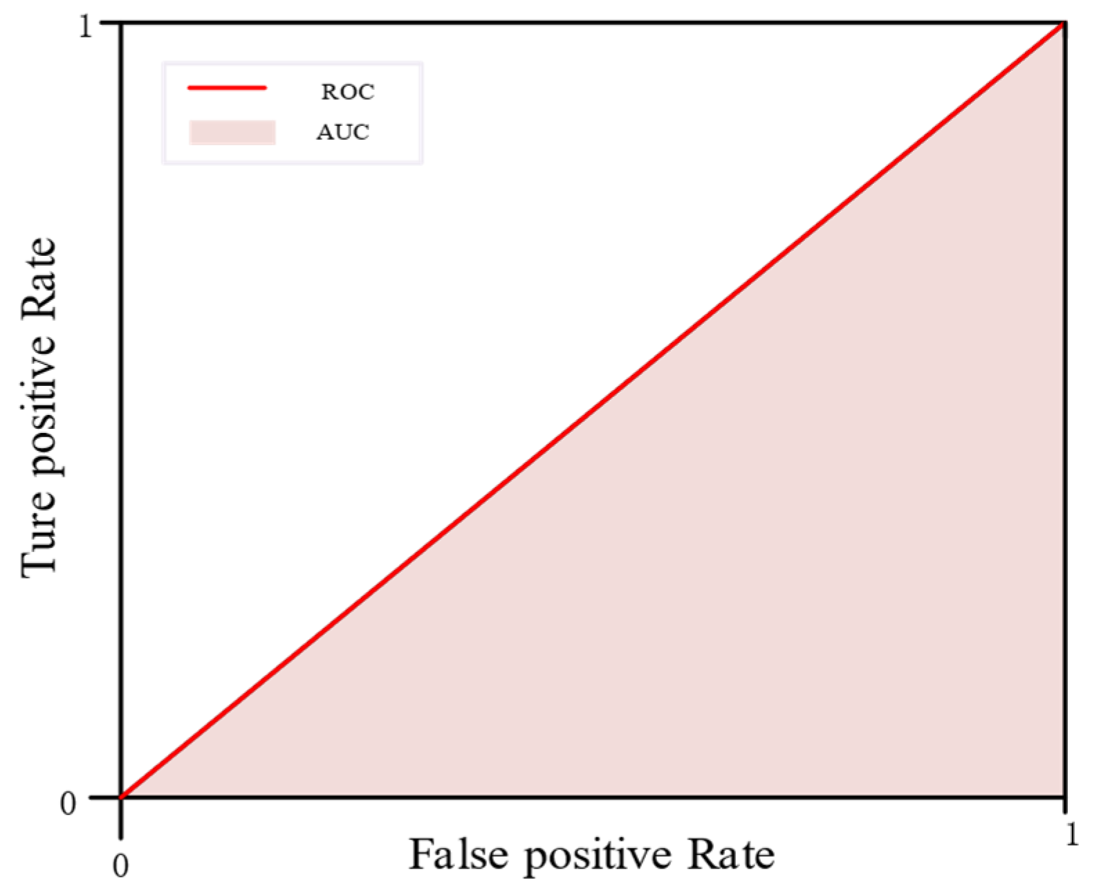
Figure 1 presents a scenario where the TPRate exceeds the FPRate. In this case, the AUC value surpasses 0.5. This implies that the model is more likely to correctly classify positive samples than to misclassify negative samples. It suggests that the model can reliably differentiate between positive and negative samples.
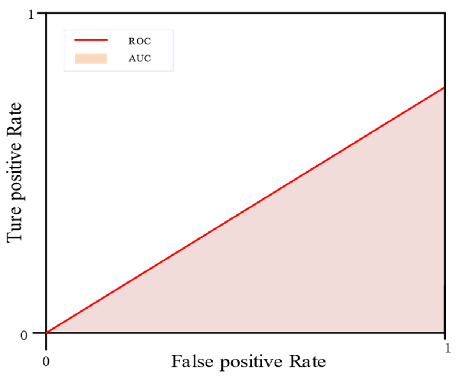
Figure 2 illustrates the scenario where the TPRate equals the FPRate, and the value of AUC stands at 0.5. In this situation, the proportion of positive samples accurately classified as positive by the ability evaluation model equals the proportion of negative samples falsely classified as positive. This suggests that the model is essentially making random predictions akin to a coin flip, unable to correctly differentiate between positive and negative samples.
Figure 3 portrays the extreme case where the TPRate is lower than the FPRate. Here, the AUC value is less than 0.5, indicating that the model is more likely to classify sample categories incorrectly. Interestingly, reversing the predicted categories in this scenario could potentially yield a capability evaluation model with an AUC greater than 0.5.
The evaluation metrics of Accuracy, F1 score, and AUC are typically employed to gauge a model’s proficiency in distinguishing positive instances in binary classification problems. However, given the multiclass nature of the ability evaluation issue addressed in this paper, relying solely on Accuracy, F1 score, and AUC for evaluation is not feasible. Consequently, we adopt a “one-vs.-one balanced” strategy (Macro Average), wherein each label serves as the positive class once, with the remaining acting as the negative class. The Accuracy, F1 score, and AUC are calculated at each iteration, followed by averaging the totals. A higher average value across Accuracy, F1 score, and AUC indicates a stronger classification performance of the ability evaluation model.

3.2. Model Construction

The capability evaluation of meteorological disaster emergency response agencies encompasses two primary components: capability feature extraction and evaluation model construction [29]. Building on this foundation, a more comprehensive capability evaluation model construction phase is developed, integrating the model extraction steps delineated in the previous section.
(1)
Capability Feature Encoding: As detailed in Equations (3)–(9), the final encoder is attained by marrying the SGD algorithm with the training of an Encoder-Decoder architecture based on the ability feature sequence set X f * .
(2)
Capability Feature Extraction: In alignment with Equation (10), feature extraction is conducted on X to realize the objective of learning the dynamic features of the sequence and reducing dimensionality, thereby deriving the new feature set A and the dimensionality-reduced data set S = ( A , Y ) .
(3)
Dataset Partitioning: Following a predetermined ratio, the dataset S is bifurcated into a training set S train   and a testing set S test   .
(4)
Model Parameter Setting: Guided by existing domestic and international research, along with insights from authoritative experts, the range for hyperparameter values is established, as delineated in Table 2.
Utilizing Equation (8), where L α A d a p t i v e F o c a l p i , y i functions as the loss function, and in accordance with Equations (9)–(17), we construct and train a deep neural network based on S train   to develop the Encoder-Adaptive-Focal-based deep neural network capability evaluation model. Employing this model, predictions are executed on S test   . The performance indices of the capability evaluation model are ascertained following Equations (18)–(21), facilitating a comprehensive assessment of its efficacy. Figure 4 illustrates the modeling workflow of the proposed capability evaluation scheme.

3.3. Performance Testing and Comparative Analysis

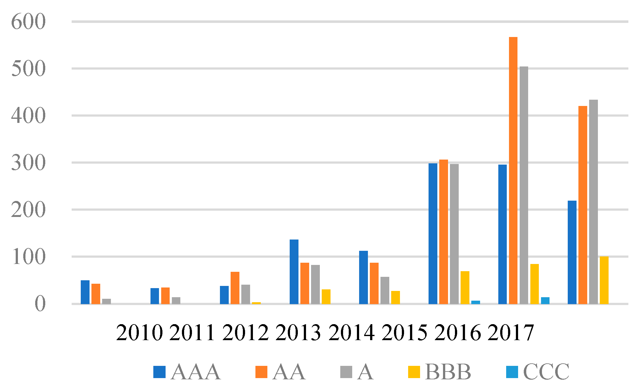
To predict the capability level of agencies that haven’t undergone evaluation, this paper’s developed model requires training using meteorological disaster emergency agencies’ capability data. Data acquisition stems from three primary sources: the government agency information publication website, the third-party capability information query platform, and records from the government oversight process. The capability evaluation results for the meteorological disaster emergency response agencies were sourced from relevant websites, using the data collection methodology described in a previous paper. These findings were cross-referenced with the capability characteristic data gathered earlier to filter out agencies with numerous missing indicators or without any capability levels. Figure 5 visualizes these results. Figure 5 vividly illustrates the capability levels of meteorological disaster emergency agencies from 2010 to 2017, as determined by different evaluations. Using a color-coded bar graph representation, the varying capability levels, categorized as AAA, AA, A, BBB, and CCC, are distinctly showcased. A cursory look at the graph reveals that 2016 witnessed a significant surge in agencies achieving the ‘AAA’ rating, indicating a pinnacle in capability and preparedness. Conversely, ‘CCC’-rated agencies, symbolizing lower capabilities, remained relatively stable and low across the years. The spikes and troughs observed across the years provide a clear insight into the evolving competency of these agencies over time. This data visualization is pivotal for comprehending the shifts in agency capabilities and for ensuring continuous improvements in the face of meteorological disasters.
Before 2015, few departments undertook capability evaluations, and even fewer received ratings below an ‘A’. The trends suggest that earlier capability rating systems and technical means were somewhat rudimentary, resulting in many meteorological departments receiving inflated capability scores [32]. However, as the capability system evolved over the years, there’s been an increase in agencies receiving “BBB” and “CCC” ratings. This trend signifies effective government oversight while also pointing to gaps in meteorological disaster defense, which pose challenges for emergency management and decision-making. Figure 5 further highlights the ongoing disparities in capability levels. The bar colors represent different ratings, with blue indicating ‘AAA’, orange ‘AA’, gray ‘A’, yellow ‘BBB’, and light blue ‘CCC’.
The 4565 competency evaluations collated were grouped based on their respective institutions, yielding a total of 2384 institutions with time series evaluation results yt. Together with the competency feature extraction results outlined earlier, they form the sample set.
Data collected in this paper, chiefly from the main capability information platforms, encompass capability characteristic data, behavior timing information, subject capability level data, and evaluation data. Combined, these elements form a comprehensive time series sample. Table 3 showcases statistics for various capability features after data pre-processing. The capability rating model crafted in this research screens out samples with incomplete or missing data, necessitating that each time series sample offers extensive capability features and maintains at least two records of capability ratings [33].

3.3.1. Comparative Analysis of Loss Function Performance

In Section 3.3.1, we analyze the performance of various loss functions through a comparative study. The sample set S , comprising various capability institutions, is utilized to pinpoint the optimal hyperparameters as delineated in Table 1; the resultant findings are cataloged in Table 4. Subsequently, the dimensionality-reduced dataset, denoted as S , is partitioned into a training set ( S train   ) and a test set S test   ) based on a 7:3 ratio. Following this, S train   is fed into the neural network, employing L α   Adaptive - Focal   p i , y i as the loss function during the training phase. This strategy facilitates the development of the Encoder-Adaptive-Focal deep neural network for dynamic capability evaluation.
To verify the efficacy of the Weighted Adaptive Focal Loss (WAFL) introduced in this study for capability evaluation, we conducted experiments to compare the Encoder-Adaptive-Focal deep neural network capability evaluation model constructed herein with Encoder-DNN and Encoder-Focal models. The comparative results are displayed in Table 5.
To further scrutinize the effectiveness of the Weighted Adaptive Focal Loss (WAFL) and to comply with the reviewer’s suggestion, we executed additional experiments employing a 60:40 training-testing split. The Encoder-Adaptive-Focal model was once again juxtaposed against the Encoder-DNN and Encoder-Focal models to ascertain any potential enhancement in performance with this altered data split. The comparative findings are encapsulated in Table 6 below.
The results delineated in Table 6 signify a marginal improvement in model performance across all three models with the 60:40 data split, particularly showcasing a slight enhancement in the Encoder-Adaptive-Focal model’s F1 score and AUC values. This exploration underscores the importance of data split ratios in honing the efficacy of our proposed model and provides a promising avenue for further optimization in our capability evaluation methodology.
In this comparison, the encoder of the Encoder-DNN model mirrors the specifications outlined in Table 7. Following the feature extraction process, a deep learning model utilizing cross-entropy loss is applied for ability level classification; the classifier hyperparameters are delineated in Table 7.
Meanwhile, the Encoder-Focal model maintains encoder parameters identical to those stipulated in Table 8. This classifier incorporates a deep learning model with five hidden layers and employs the focal loss function described in Equation (4) as the loss function, adhering to the hyperparameter configurations indicated in Table 8.
As deduced from the data in Table 5, the application of the WAFL loss function devised in this study notably enhances the performance metrics of the capability evaluation model, surpassing the outcomes of the neural network model devoid of the augmented loss function and the incorporation of focus parameters. Furthermore, there is a significant enhancement in the recognition accuracy of low-ability-level samples, achieving a recognition accuracy rate of 92.7% for samples under ability level A. This surpasses the 68.4% and 81.3% recognition accuracy rates achieved by the other two models, substantiating that refining cross entropy through adaptive focus and sample weights augments the emphasis on key samples.

3.3.2. Subsubsection

To validate the efficacy of integrating the RNN feature extraction method with the focal loss function, we contrasted the Encoder-Adaptive-Focal deep neural network capability evaluation model developed in this study against both the Adaptive-Focal and PCA-Adaptive-Focal models in separate tests. Given that neither the Adaptive-Focal nor the PCA-Adaptive-Focal models employed an RNN encoder for feature extraction, and thus couldn’t procure time-series features, the capability features from the most recent instance were utilized for the sample features. Table 9 presents the performance metrics for each model.
The Adaptive-Focal model lacks a feature extractor and solely uses the initial set of capability features (24 indicators) previously constructed as its input. The classifier’s hyperparameters are as defined in Table 4.
For the PCA-Adaptive-Focal model, the method of dimensionality reduction employed is PCA. The first three principal components from the most recent capability feature set are taken as the capability features for the sample, with their combined variance contribution exceeding 85%. The classifier’s hyperparameters remain consistent with those listed in Table 4.
As per the comparison results presented in Table 8, the RNN encoder dimensionality reduction method utilized in this study has proven to be more effective at enhancing model performance than the non-dimensioned and PCA methods. Notably, there’s a 5% increase in accuracy metrics and an 11.4% rise in AUC compared to the PCA method. The accuracy and AUC metrics of the PCA-Adaptive-Focal are marginally lower than the Adaptive-Focal. This is because the PCA method not only neglects the temporal data features but also loses some information from the most recent period, leading to reduced classification accuracy.

3.3.3. Classifier Comparison

To validate the suitability of implementing a deep neural network model for capability evaluation in this research, we compared the Encoder-Adaptive-Focal deep neural network capability evaluation model developed here with Encoder-DecisionTree, Encoder-SVM, and Encoder-NaiveBayes models in separate trials. The outcomes of these comparisons can be found in Table 10.
The encoder parameters for the Encoder-DecisionTree model are specified in Table 7, with the classifier utilizing the CART model and hyperparameters outlined in Table 11.
The Encoder-SVM model adopts the capability feature extraction methodology introduced in the previous paper. These extracted feature values serve as inputs for the random forest model during capability evaluation model training. Parameter settings for feature extraction mirror those in Table 7, while the classifier’s hyperparameters adhere to Table 12.
The Encoder-NaiveBayes model employs basic Bayes for capability assessment. Encoder parameters are set according to Table 7. The classifier is NaiveBayes, negating the need for hyperparameter tuning [34].
A review of the findings in Table 11 reveals that, for intricate classification tasks like the capability evaluation of meteorological disaster response agencies, deep neural network-based evaluation methods surpass traditional, mathematical, statistics-based approaches. Models such as Encoder-DecisionTree, Encoder-SVM, and Encoder-NaiveBayes not only exhibit reduced Accuracy and F1 scores compared to the Encoder-Adaptive-Focal method of this paper, but their AUCs also hover near 0.5. This suggests that mathematical, statistics-based evaluation methods might falter when faced with classification challenges involving imbalanced sample categories.
Upon a comprehensive analysis and juxtaposition of data showcased in Table 5, Table 8 and Table 9, a notable supremacy of the Encoder-Adaptive-Focal deep neural network approach in dynamic capability rating becomes palpable. This study underscores the model’s proficiency at transcending conventional assessment paradigms.
At its core, this method exhibits a heightened capability in the extraction of nuanced features from time series data, a critical step that facilitates a deeper insight into the evolving dynamics of meteorological phenomena. Notably, it adeptly compresses the dimensionality of these features, thereby alleviating computational burdens and paving the path for more streamlined analyses.
Moreover, an ingenious aspect of this approach lies in its ability to recalibrate the focal point of the evaluation model. Moving beyond a mere quantitative analysis, it navigates away from the simple and anomalous samples, channeling its focus toward the more challenging, yet insightful data pockets [35]. This nuanced shift in focus not only nurtures a richer analytical depth but also engenders a more holistic understanding of the meteorological disaster capability spectra.
A meticulous scrutiny of the model’s performance metrics, namely Accuracy, F1 score, and AUC values, reveals its unparalleled superiority. It emerges as a method that is fine-tuned to navigate the complexities inherent in meteorological disaster capability assessments, embodying a harmonious blend of precision and depth.
Furthermore, it would be remiss of the authors not to acknowledge the potential implications of this approach in crafting proactive and responsive disaster management strategies. Offering a more granular view of meteorological disaster capabilities equips policymakers and stakeholders with actionable insights, fostering a climate of informed decision-making and strategic foresight.
Thus, as evidenced by its robust performance metrics and analytical depth, the Encoder-Adaptive-Focal deep neural network approach emerges as a pivotal tool in the realm of meteorological disaster capability assessments. It stands as a testament to the potential of leveraging advanced neural network techniques in forging pathways toward more resilient and adaptive disaster management frameworks.
The degree of training accuracy is a pivotal parameter that reflects the model’s aptitude for effective learning from the provided training dataset. Throughout the course of this study, we meticulously monitored the training accuracy across various models to ensure a robust learning trajectory. Our Encoder-Adaptive-Focal model demonstrated an exemplary training accuracy, signifying its enhanced learning capability. We have elucidated the detailed training accuracy metrics in the revised manuscript, facilitating a clearer understanding of the models’ learning efficacy and providing a foundation for the subsequent comparative analyses.
The F1 score and Area Under the Receiver Operating Characteristic Curve (AUC) are indispensable metrics for evaluating the performance of models, especially in scenarios characterized by imbalanced datasets, akin to our study. Our proposed Encoder-Adaptive-Focal model yielded an appreciable F1 score and AUC value, denoting its ability to adeptly handle sample imbalance and achieve reliable classification outcomes. The expanded discussion on these metrics within the revised manuscript offers a more nuanced comprehension of the models’ effectiveness and their implications for the capability evaluation of meteorological disaster response agencies.
We have enriched the comparative analysis to furnish a more holistic understanding of the relative merits and demerits of the proposed and existing models. The juxtaposition predicated on key performance metrics such as Accuracy, F1 score, and AUC values furnishes a comprehensive view of the models’ performance. This augmented comparative analysis aims to bolster the justification for the results obtained, illuminating the superior performance of the Encoder-Adaptive-Focal model in addressing the cardinal challenge of sample imbalance.
The implications of the models’ performance transcend the theoretical ambit, venturing into the pragmatic domain of disaster management. The superior metrics exhibited by our proposed model underscore its potential in affording actionable insights to policymakers and stakeholders. This enhanced discussion on the implications, now included in the revised manuscript, expounds on how the findings could contribute to the formulation of more proactive and responsive disaster management strategies, thereby representing a significant stride toward augmenting meteorological disaster capability assessments.
A survey of contemporary literature underscores a predominant reliance on traditional neural network models and linear regression techniques. While these methodologies have their merits, they often fall short of capturing the intricate dynamics inherent in meteorological data. The Encoder-Adaptive-Focal model, on the other hand, is uniquely equipped to handle such complexities, a fact that becomes evident when it is juxtaposed with the outcomes of these conventional models.
Furthermore, the recent surge in interest around convolutional neural networks (CNNs) and recurrent neural networks (RNNs) in meteorological studies should be acknowledged. These models, though sophisticated, often require extensive computational resources and, at times, may not be adept at managing the nuances of time series data, especially in the context of meteorological disaster capabilities. In contrast, our proposed approach strikes an optimal balance, maximizing efficiency without compromising on depth and precision.
It’s also crucial to highlight the seminal works of researchers who have paved the way in this field with their groundbreaking methodologies. While their contributions have undeniably shaped the trajectory of disaster capability assessments, the Encoder-Adaptive-Focal model’s adaptive nature and recalibration mechanisms offer a fresh perspective, potentially setting a new benchmark in the domain.
In conclusion, by integrating insights from the extant literature and highlighting the novel facets of the Encoder-Adaptive-Focal deep neural network approach, we hope to enrich the academic discourse. This comparative analysis not only solidifies our model’s position within the research landscape but also underscores its potential in reshaping the future of meteorological disaster capability assessments.

4. Conclusions

Meteorological disasters like hurricanes, floods, and droughts wield a potentially devastating impact on communities, infrastructure, and the economy. Thus, devising robust and effective strategies for disaster management and response is not only paramount but a requisite for safeguarding the welfare of the populace and economic stability. A central facet of these strategies hinges on the accurate evaluation of the defense capacity of towns and regions, a practice instrumental in enhancing disaster management efficacy.
Yet, the journey toward precision in evaluation encounters stumbling blocks, primarily due to the pervasive issue of sample imbalance in the datasets leveraged for these evaluations. This imbalance, characterized by a disparate ratio of positive to negative outcomes (disaster and non-disaster events), threatens to skew the evaluations, rendering them less reflective of the actual defense capabilities.
In response to this challenge, this research innovatively melds the adaptive focal loss with the cross-entropy loss function, pioneering a nuanced approach to tackling the sample imbalance problem. This paper not only elucidates the intricate process of information collection and parsing necessary for dynamic capability evaluation but also charts the blueprint of the Encoder-Adaptive-Focal deep learning dynamic evaluation model. A thorough comparison of this model’s metrics with existing evaluation methods across three distinct dimensions underscores its superior applicability and effectiveness in capability assessment.
As we venture forward, addressing the sample imbalance in meteorological disaster defense capability evaluation emerges as a critical milestone. The advent of methodologies capable of counteracting this imbalance heralds a new era of precision in evaluating defense capabilities. This, in turn, promises to catalyze the evolution of disaster management strategies, steering them toward heightened effectiveness. By fostering more accurate evaluations, we pave the way for fortified disaster response strategies, aiming to significantly diminish the damages wrought by meteorological disasters and fostering a safer and more resilient future.

Author Contributions

Conceptualization, J.T. and R.S.; methodology, J.T. and R.S.; software, J.T. and Q.D.; validation, J.T., R.S., Q.D. and Y.M.; formal analysis, J.T. and R.S.; investigation, J.T.; resources, J.T.; data curation, J.T.; writing—original draft preparation, J.T. and Q.D.; writing—review and editing, J.T., R.S. and Y.M.; visualization, J.T.; supervision, R.S. and Y.M.; project administration, Q.D. and Y.M. All authors have read and agreed to the published version of the manuscript.

Funding

This work was supported by Research project of State Grid Corporation (4000-202318098A-1-1-ZN). The authors would like to acknowledge Osaka Metropolitan University for providing the materials used for experiments.

Institutional Review Board Statement

Not applicable.

Informed Consent Statement

Not applicable.

Data Availability Statement

Data are contained within the article.

Acknowledgments

We would like to express our gratitude to the journal editors and reviewers for the recognition of this paper and the comments and suggestions which are invaluable for the improvement of our manuscript.

Conflicts of Interest

The authors declare that they have no known competing financial interests or personal relationships that could have appeared to influence the work reported in this paper. Qiangsheng Dai is employee of State Grid Jiangsu Electric Power Co., Ltd., who provided funding and teachnical support for the work. The funder had no role in the design of the study; in the collection, analysis, or interpretation of data, in the writing of the manuscript, or in the decision to publish the results.

Appendix A

import numpy as np
import tensorflow as tf

epoch = 10
num_feature=3
num_lable =5
ru = 0.5
data=np.loadtxt("data/credit.csv",dtype=np.float,delimiter=',')

def weight_dict (data,num_feature=3,num_lable =5):
  sample,column = np.shape(data)
  weight_dict ={}
  if column-num_feature == num_lable:
   for label in np.arange(0,column)[num_feature:]:
    #print(label)
    ones = np.ones([1,sample])
    same_class = np.sum(ones × data[:,label])
    weight_dict[label-num_feature]=(sample − same_class)/sample

  else:
   print(")
  return weight_dict

alpha = tf.placeholder(tf.float32)
s = tf.placeholder(tf.float32)
X = tf.placeholder(tf.float32,[None,3])
Y = tf.placeholder(tf.float32,[None,5])

w1 = tf.Variable(tf.truncated_normal([3,7],stddev=0.1))
w2 = tf.Variable(tf.truncated_normal([7,5],stddev=0.1))
w3 = tf.Variable(tf.truncated_normal([5,5],stddev=0.1))
w4 = tf.Variable(tf.truncated_normal([5,3],stddev=0.1))
w5 = tf.Variable(tf.truncated_normal([3,5],stddev=0.1))

b1 = tf.Variable(tf.zeros([7]))
b2 = tf.Variable(tf.zeros([5]))
b3 = tf.Variable(tf.zeros([5]))
b4 = tf.Variable(tf.zeros([3]))
b5 = tf.Variable(tf.zeros([5]))

L1 = tf.nn.relu(tf.matmul(X,w1)+b1)
L2 = tf.nn.relu(tf.matmul(L1,w2)+b2)
L3 = tf.nn.relu(tf.matmul(L2,w3)+b3)
L4 = tf.nn.relu(tf.matmul(L3,w4)+b4)
L5 = tf.nn.softmax(tf.matmul(L4,w5)+b5)

loss = alpha*s*tf.nn.softmax_cross_entropy_with_logits(labels=Y,logits=L5)

train_step = tf.train.GradientDescentOptimizer(0.5).minimize(loss)

init = tf.global_variables_initializer()
sess = tf.Session()
sess.run(init)
weight_diction = weight_dict(data)

# diff = [0]
# si =[0]
# y_p = []
sample, column = np.shape(data)

diff = np.ones([epoch+1,sample],dtype=np.float32)
si =np.ones([epoch+1,sample],dtype=np.float32)
y_p =np.zeros([epoch+1,sample],dtype=np.float32)
for e in range(3):
  sample, column = np.shape(data)

  for i in range(sample):
    # current_epoch_yp = []
    # current_epoch_diff = []
    X_onesample=np.expand_dims(data[i, 0:num_feature],0)
    Y_onesample = np.expand_dims(data[i,num_feature:column],0)
    current_sample_class =0
    for j in range(num_lable):
      if j ==1:
        current_sample_class = j
      break
    loss1,out = sess.run([loss,L5],feed_dict={X:X_onesample,Y:Y_onesample,alpha:weight_diction[current_sample_class],s:1})
    current_y_p = np.sum(np.abs(data[i,num_feature:column]-out))

    y_p[e][i] = current_y_p

  diff[2] = np.abs(y_p[1]-y_p[2])
  diff[1] =np.abs(y_p[1]-y_p[0])
  si[2] = ru*si[1] +(1-ru)*diff[1]
  si[3] = ru*si[2] +(1-ru)*diff[2]
  print(si[3])
for e in range(3,epoch):

  for i in range(sample):
    X_onesample=np.expand_dims(data[i, 0:num_feature],0)
    Y_onesample = np.expand_dims(data[i,num_feature:column],0)
    current_sample_class =0
    for j in range(num_lable):
      if j ==1:
        current_sample_class = j
        break
    loss1,out = sess.run([loss,L5],feed_dict={X:X_onesample,Y:Y_onesample,alpha:weight_diction[current_sample_class],s:si[epoch][i]})
    current_y_p = np.sum(np.abs(data[i,num_feature:column]-out))
    y_p[e,i] = current_y_p
    # diff.append(y_p[-1] - y_p[-2])
    y_p[e,i] = current_y_p
  diff[e] = np.abs(y_p[e] - y_p[e-1])

  si[e+1] = ru * si[e] + (1 - ru) * diff[e]
  print(si[e+1])
  print(loss1)

References

  1. Baihaqi, L.H. The Role of Yonzipur 9/LLB/1 Kostrad in the Earthquake Emergency Response Phase (Case Study of Earthquake Disaster in Cianjur). Int. J. Soc. Sci. Res. 2023, 3, 1489–1693. [Google Scholar] [CrossRef]
  2. Bryen, D.N. Communication during times of natural or man-made emergencies. J. Pediatr. Rehabil. Med. 2009, 2, 123–129. [Google Scholar] [CrossRef]
  3. Corbacioglu, S.; Kapucu, N. Organisational learning and self-adaptation in dynamic disaster environments. Disasters 2006, 30, 212–233. [Google Scholar] [CrossRef]
  4. Mah Hashim, N.; Abu Bakar, N.A.; Kamaruzzaman, Z.A.; Shariff, S.R.; Burhanuddin, S.N.Z.A. Flood Governance: A Review on Allocation of Flood Victims Using Location-Allocation Model and Disaster Management in Malaysia. J. Geogr. Inf. 2023, 6, 493–503. [Google Scholar] [CrossRef]
  5. Zantal-Wiener, K.; Horwood, T.J. Logic modeling as a tool to prepare to evaluate disaster and emergency preparedness, response, and recovery in schools. New Dir. Eval. 2010, 2010, 51–64. [Google Scholar] [CrossRef]
  6. Wang, J.F.; Feng, L.J.; Zhai, X.Q. A system dynamics model of flooding emergency capability of coal mine. Prz. Elektrotechniczny 2012, 88, 209–211. [Google Scholar]
  7. Sugumaran, V.; Wang, X.Z.; Zhang, H.; Xu, Z. A capability assessment model for emergency management organizations. Inf. Syst. Front. 2017, 20, 653–667. [Google Scholar] [CrossRef]
  8. Kyrkou, C.; Kolios, P.; Theocharides, T.; Polycarpou, M. Machine Learning for Emergency Management: A Survey and Future Outlook. Proc. IEEE 2023, 111, 19–41. [Google Scholar] [CrossRef]
  9. Herlianto, M. Early Disaster Recovery Strategy: The Missing Link in Post-Disaster Implementation in Indonesia. Influ. Int. J. Sci. Rev. 2023, 5, 80–91. [Google Scholar] [CrossRef]
  10. Love, P.E.D.; Matthews, J. Quality, requisite imagination and resilience: Managing risk and uncertainty in construction. Reliab. Eng. Syst. Saf. 2020, 204, 12. [Google Scholar] [CrossRef]
  11. Hosseini, A.; Faheem, A.; Titi, H.; Schwandt, S. Evaluation of the long-term performance of flexible pavements with respect to production and construction quality control indicators. Constr. Build. Mater. 2020, 230, 9. [Google Scholar] [CrossRef]
  12. Francom, T.; Markham, C. Identifying Geotechnical Risk and Assigning Ownership on Water and Wastewater Pipeline Projects using Alternative Project Delivery Methods. In Proceedings of the Sessions of the Pipelines Conference, Phoenix, AZ, USA, 6–9 August 2017; Amer Soc Civil Engineers: New York, NY, USA, 2017; pp. 494–503. [Google Scholar]
  13. Yao, J.; Yan, L.; Xu, Z.; Wang, P.; Zhao, X. Collaborative Decision-Making Method of Emergency Response for Highway Incidents. Sustainability 2023, 15, 2099. [Google Scholar] [CrossRef]
  14. Shen, L.; Zhang, Z.; Tang, L. Study on Key Drivers and Collaborative Management Strategies for Construction and Demolition Waste Utilization in New Urban District Development: From a Social Network Perspective. J. Environ. Public Health 2023, 2023, 3660647. [Google Scholar] [CrossRef]
  15. Liu, Z.; Ma, L. Introduction of the Special Issue on Building Digital Government in China. Commun. ACM 2022, 65, 64–66. [Google Scholar] [CrossRef]
  16. Wang, C.J.; Ng, C.Y.; Brook, R. Response to COVID-19 in Taiwan: Big Data Analytics, New Technology, and Proactive Testing. JAMA 2020, 323, 1341–1342. [Google Scholar] [CrossRef]
  17. Heidary Dahooie, J.; Razavi Hajiagha, S.H.; Farazmehr, S.; Zavadskas, E.K.; Antucheviciene, J. A novel dynamic credit risk evaluation method using data envelopment analysis with common weights and combination of multi-attribute decision-making methods. Comput. Oper. Res. 2021, 129, 105223. [Google Scholar] [CrossRef]
  18. He, Y.; Xu, Z.; Gu, J. An approach to group decision making with hesitant information and its application in credit risk evaluation of enterprises. Appl. Soft Comput. 2016, 43, 159–169. [Google Scholar] [CrossRef]
  19. Shen, F.; Ma, X.; Li, Z.; Xu, Z.; Cai, D. An extended intuitionistic fuzzy TOPSIS method based on a new distance measure with an application to credit risk evaluation. Inf. Sci. 2018, 428, 105–119. [Google Scholar] [CrossRef]
  20. Shen, F.; Zhao, X.; Kou, G.; Alsaadi, F.E. A new deep learning ensemble credit risk evaluation model with an improved synthetic minority oversampling technique. Appl. Soft Comput. 2021, 98, 106852. [Google Scholar] [CrossRef]
  21. Wang, L.; Wu, C. Dynamic imbalanced business credit evaluation based on Learn++ with sliding time window and weight sampling and FCM with multiple kernels. Inf. Sci. 2020, 520, 305–323. [Google Scholar] [CrossRef]
  22. Huang, X.; Liu, X.; Ren, Y. Enterprise credit risk evaluation based on neural network algorithm. Cogn. Syst. Res. 2018, 52, 317–324. [Google Scholar] [CrossRef]
  23. Cai, X.; Qian, Y.; Bai, Q.; Liu, W. Exploration on the financing risks of enterprise supply chain using Back Propagation neural network. J. Comput. Appl. Math. 2020, 367, 112457. [Google Scholar] [CrossRef]
  24. Ioffe, S.; Szegedy, C. Batch Normalization: Accelerating Deep Network Training by Reducing Internal Covariate Shift. JMLR.org 2015, 37, 448–456. [Google Scholar]
  25. Kingma, D.; Ba, J. Adam: A Method for Stochastic Optimization. arXiv 2014, arXiv:1412.6980. [Google Scholar]
  26. Chawla, N.V.; Bowyer, K.W.; Hall, L.O.; Kegelmeyer, W.P. SMOTE: Synthetic minority oversampling technique. J. Artif. Intell. Res. 2002, 16, 321–357. [Google Scholar] [CrossRef]
  27. Graves, A.; Mohamed, A.R.; Hinton, G. Speech Recognition with Deep Recurrent Neural Networks. In Proceedings of the Acoustics Speech & Signal Processing International Conference, Vancouver, BC, Canada, 26–31 May 2013. [Google Scholar] [CrossRef]
  28. Hinton, G.E.; Salakhutdinov, R.R. Reducing the dimensionality of data with neural networks. Science 2006, 313, 504–507. [Google Scholar] [CrossRef]
  29. Ahmad, A.M.; Ismail, S.; Samaon, D.F. Recurrent Neural NETWORK with Backpropagation through Time for Speech Recognition. In Proceedings of the IEEE International Symposium on Communications and Information Technology, Sapporo, Japan, 26–29 October 2004; IEEE: New York, NY, USA, 2005. [Google Scholar] [CrossRef]
  30. Liu, Y.; Zhong, D.; Cui, B.; Zhong, G.; Wei, Y. Study on real-time construction quality monitoring of storehouse surfaces for RCC dams. Autom. Constr. 2015, 49, 100–112. [Google Scholar] [CrossRef]
  31. Chen, F.; Jiao, H.; Han, L.; Shen, L.; Du, W.; Ye, Q.; Yu, G. Real-time monitoring of construction quality for gravel piles based on Internet of Things. Autom. Constr. 2020, 116, 103228. [Google Scholar] [CrossRef]
  32. Ma, Z.; Cai, S.; Mao, N.; Yang, Q.; Feng, J.; Wang, P. Construction quality management based on a collaborative system using BIM and indoor positioning. Autom. Constr. 2018, 92, 35–45. [Google Scholar] [CrossRef]
  33. AL-Sahar, F.; Przegalińska, A.; Krzemiński, M. Risk assessment on the construction site with the use of wearable technologies. Ain Shams Eng. J. 2021, 12, 3411–3417. [Google Scholar] [CrossRef]
  34. Qing, L.; Rengkui, L.; Jun, Z.; Quanxin, S. Quality Risk Management Model for Railway Construction Projects. Procedia Eng. 2014, 84, 195–203. [Google Scholar] [CrossRef]
  35. Gu, J.; Xia, X.; He, Y.; Xu, Z. An approach to evaluating the spontaneous and contagious credit risk for supply chain enterprises based on fuzzy preference relations. Comput. Ind. Eng. 2017, 106, 361–372. [Google Scholar] [CrossRef]
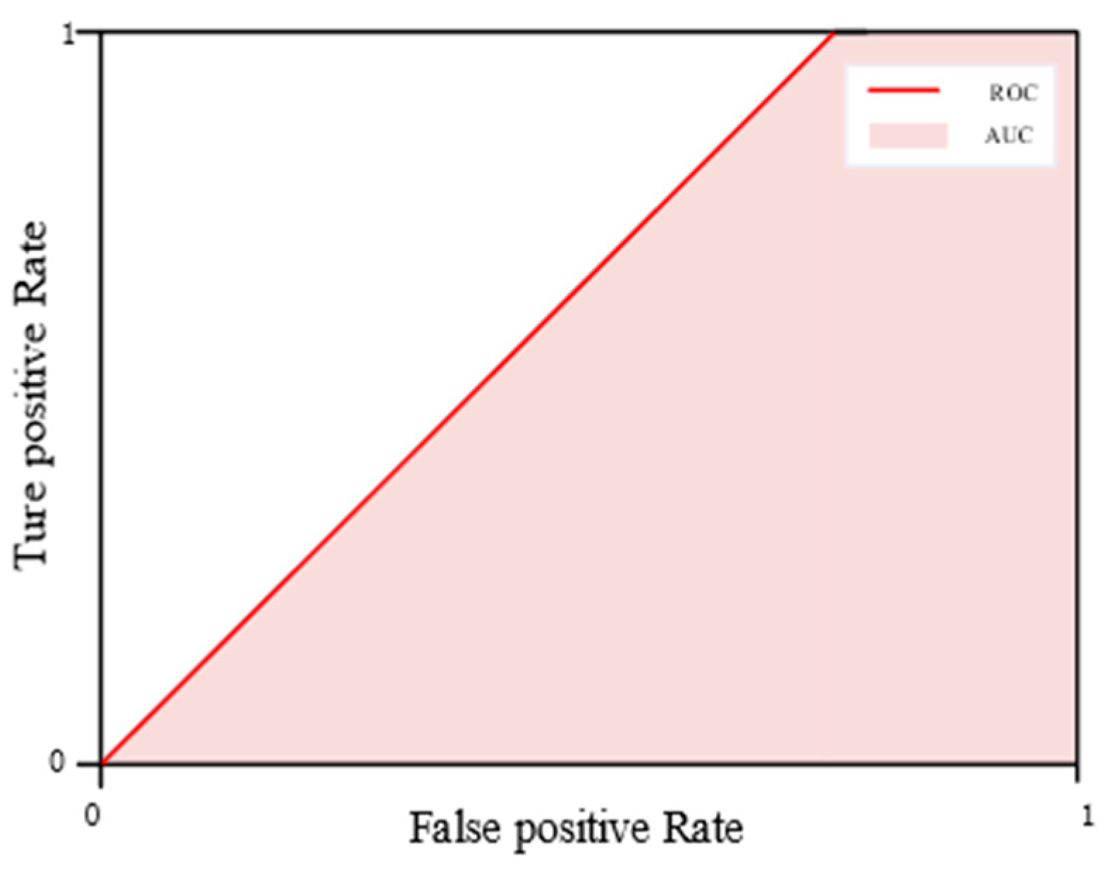
Figure 1. Scenario where TPRate is greater than FPRate.
Applsci 13 12561 g001
Figure 2. Scenario where TPRate equals FPRate.
Applsci 13 12561 g002
Figure 3. Scenario where TPRate is smaller than FPRate.
Applsci 13 12561 g003
Figure 4. Modeling process of weather disaster emergency response capacity evaluation model.
Applsci 13 12561 g004
Figure 5. Annual distribution of competence levels.
Applsci 13 12561 g005
Table 1. Confusion matrix.
Prediction/Real10
1True (TP)False Negative (FN)
0False Positive (FP)True Negative (TN)
Table 2. Value range of hyperparameters.
HyperparametersMeaningRoleRange of Values
LayersNumber of neural network layersChange the complexity of the model[4, 7].
C l Number of neurons in layer lChange the complexity of the model[4, 8].
g l The activation function of the lth layerLearning non-linear relationships{Relu, Tanh, Sogmoid, Softmax}
BBatch size of input samples per training roundTrade-off between model accuracy and training efficiency{16, 32, 64}
ENumber of model training roundsMake the model continuously learn the distribution of the training data[100, 500]
εLearning RateControl the step size of the weight update{0.001, 0.005, 0.01, 0.05}
oAdaptive learning rate algorithmAutomatically adjust the learning rate according to some strategy to find the global optimal point{SGD, AdaGrad, RMSProp, Adam}
ρ Correction factorControl d i f f i ( e ) for s i The correction magnitude of{0.2, 0.5, 0.8}
Table 3. Statistics of some ability characteristics.
Automatic Weather Station Coverage RateHydrographic Station Network DensityWeather Radar Station CoverageNumber of Flood Control WorksRatio of Lightning Protection Device InstallationClean Water Guarantee NumberNumber of Spare Generating SetsOrganizational System Construction StatusInformation Release ManagementWeather Disaster Emergency Regulations Construction Number of SheltersNumber of Doctors per 1000 PeopleStatus of Disaster Information Dissemination AwarenessCommand Staff Quality
Number of samples40524052405240524052405240524052405240524052405240524052
Average value0.0290.0100.0580.0090.0050.0110.0150.0400.0230.0190.0160.0030.0050.012
Variance0.0480.0340.0790.0450.0380.0490.0590.0610.0820.0600.0380.0230.0350.031
Minimum value00000000000000
25% quantile00000000000000
5 quintiles0.01600.04300000.008000000
75th percentile0.0360.0065790.08600000.086000000
Maximum value11111111111111
Table 4. Hyperparameter search results.
HyperparametersValue
Layers5
C l 7, 5, 5, 3, 5, respectively
g l Relu for the hidden layer and Softmax for the output layer
B64
E300
ε0.005
oAdam
ρ 0.5
Table 5. Initial Comparison of Loss Functions in Different Models.
Models/PerformanceAccuracyF1 ScoreAUC
Encoder-Adaptive-Focal0.8440.8960.713
Encoder-DNN0.8280.8750.652
Encoder-Focal0.8360.8830.719
Table 6. Enhanced Comparison of Loss Functions with 60:40 Training-Testing Split.
Models/PerformanceAccuracyF1 ScoreAUC
Encoder-Adaptive-Focal0.8520.9040.725
Encoder-DNN0.8350.8810.665
Encoder-Focal0.8430.8890.731
Table 7. Classifier hyperparameter settings for Encoder-DNN model.
HyperparametersValue
Layers5
C l 7, 5, 5, 3, 5, respectively
g l Relu for the hidden layer and Softmax for the output layer
B64
E300
ε0.005
oAdam
ρ 0.5
Table 8. Classifier hyperparameter settings for Encoder-Focal model.
HyperparametersValue
Layers5
C l 7, 5, 5, 3, 5, respectively
g l Relu for the hidden layer and Softmax for the output layer
B64
E300
ε0.005
oAdam
γ 0.5
Table 9. Comparison results of dimensionality reduction methods.
Models/PerformanceAccuracyF1 ScoreAUC
Encoder-Adaptive-Focal0.8440.8960.713
Adaptive-Focal0.8190.8620.641
PCA-Adaptive-Focal0.8010.8650.628
Table 10. Performance Comparison of Deep Neural Network and Traditional Models.
Models/PerformanceAccuracyF1 scoreAUC
Encoder-Adaptive-Focal0.8440.8960.713
Encoder-DecisionTree0.7810.8500.533
Encoder-SVM0.7760.8490.526
Encoder-NaiveBayes0.7730.8450.522
Table 11. Classifier hyperparameter settings for Encoder-DecisionTree model.
HyperparametersMeaningValue
max_depthMaximum depth of the tree2
criterionConditions for delineating nodesgini
bootstrapSelf-help methodTrue
min_samples_splitMinimum number of samples in the node dataset10
min_samples_leafNumber of samples in leaf nodes at least6
max_leaf_nodesThe maximum number of leaf nodes the model can have4
Table 12. Classifier hyperparameter settings for Encoder-SVM model.
HyperparametersMeaningValue
kernelKernel functionsRBF
gammaCoefficients of the kernel function0.33
CPenalty coefficient of the objective function1.0
Disclaimer/Publisher’s Note: The statements, opinions and data contained in all publications are solely those of the individual author(s) and contributor(s) and not of MDPI and/or the editor(s). MDPI and/or the editor(s) disclaim responsibility for any injury to people or property resulting from any ideas, methods, instructions or products referred to in the content.