The Unmanned Aerial Vehicle (UAV)-Based Hyperspectral Classification of Desert Grassland Plants in Inner Mongolia, China

Abstract

In recent years, grassland ecosystems have faced increasingly severe desertification, which has caused continuous changes in the vegetation composition in grassland ecosystems. Therefore, effective research on grassland plant taxa is crucial to exploring the process of grassland desertification. This study proposed a solution by constructing a UAV hyperspectral remote sensing system to collect the hyperspectral data of various species in desert grasslands. This approach overcomes the limitations of traditional grassland survey methods such as a low efficiency and insufficient spatial resolution. A streamlined 2D-CNN model with different feature enhancement modules was constructed, and an improved depth-separable convolution approach was used to classify the desert grassland plants. The model was compared with existing hyperspectral classification models, such as ResNet34 and DenseNet121, under the preprocessing condition of data downscaling by combining the variance and F-norm². The results showed that the model outperformed the other models in terms of the overall classification accuracy, kappa coefficient, and memory occupied, achieving 99.216%, 98.735%, and 16.3 MB, respectively. This model could effectively classify desert grassland species. This method provides a new approach for monitoring grassland ecosystem degradation.

1. Introduction

Natural grasslands play a critical role in maintaining the ecological balance of global terrestrial ecosystems [1], accounting for more than 30% of the total ecosystem. However, with global climate change and human activities, more than half of grasslands are severely threatened by desertification [2,3]. The Inner Mongolia Autonomous Region has the largest proportion of grasslands in China, with a total natural grassland area of 8.6 × 10¹¹ m², approximately 90% of which is severely degraded [4,5]. Desert grasslands are representative of the degradation process from grassland to desert, which not only changes the original grassland communities and reduces biodiversity, but also severely affects the normal functions of grassland ecosystems, such as climate regulation, soil conservation, and biodiversity [6,7,8]. The degradation of desert grasslands can be accurately evaluated and managed by studying their taxonomy.

Currently, most traditional grassland surveys are conducted manually in the field. Although this method is more accurate, it is time-consuming and cannot be extended to cover large areas [9]. To achieve the long-term rapid monitoring of grassland features over large areas, researchers have developed experimental methods for satellite remote sensing. Although satellite remote sensing has become an essential tool for grassland monitoring because of its large spatial scale and ability to identify the spatial and temporal dynamics of grasslands, the spatial resolution of images captured with satellite remote sensing is relatively low. It can only accurately identify vegetation at large spatial scales, and its images and spectral features are submerged in mixed pixels of small- and medium-sized vegetation in desert grasslands. Satellite remote sensing is affected by the motion of satellites around the Earth, and the interval between repeated experiments is too long [10,11,12]. Therefore, more sophisticated remote sensing equipment needs to be deployed or used to achieve a finer classification of desert grassland vegetation.

In recent years, with the continuous development of unmanned aerial vehicle (UAV) technology, it has become well-known to the general public for its simple operation methods, low cost of use, and access to areas that are difficult for humans to reach [13]. Advances in optical technology have led to the development of portable hyperspectral imagers that offer higher spatial and spectral resolutions and a more prosperous continuous spectral band than satellite remote sensing. This provides a higher recognition accuracy for delineating fine features. In contrast to traditional RGB color images, hyperspectral images can unveil more hidden features within invisible bands, which are crucial for the classification and monitoring of desert grassland plants. The capability of hyperspectral imaging to intricately distinguish and capture the spectral properties of matter in minute detail renders it a powerful tool in fields such as ecology, agriculture, and environmental science. Using UAVs as platforms to carry portable hyperspectral imagers, the two can complement each other to build low-altitude UAV remote-sensing platforms [14,15,16,17]. This platform is now widely used in vegetation cover calculations [18], agricultural precision management [19], vegetation leaf area monitoring [20], and vegetation condition monitoring [21,22], among other applications.

In hyperspectral remote sensing image processing, the vegetation index method is commonly used to calculate the numerical indicators of the reflectance or radiation of features in remotely sensed images. It is used to assess the growth status of objects and vegetation cover and to monitor vegetation changes on the land surface [23,24,25,26]. These vegetation indices are dimensionless values [27]. By conducting vegetation index calculations on hyperspectral images, the most appropriate separability threshold for each feature is determined based on the calculation results, thereby completing the task of classifying image features. The most widely used vegetation indices include the Normalized Difference Vegetation Index (NDVI) [28], Ratio Vegetation Index (RVI) [29], Difference Vegetation Index (DVI) [30], and Soil-Adjusted Vegetation Index (SAVI) [31], among others. Researchers have improved commonly used vegetation indices and explored several practical applications. Ref. [32] studied the leaf area index of winter wheat in arid areas and used first- and second-order differential data preprocessing to construct two-dimensional and three-dimensional vegetation indices by combining arbitrary wavebands. The results showed that the correlation between vegetation and leaf area indices formed by combining wavebands was significantly improved. Ref. [33] constructed a microplaque index threshold (MPI-T) for the problem in which NDVI and SAVI are difficult to distinguish between desert grassland rat holes and achieved positive recognition results. However, the vegetation index calculation method has limitations and cannot fully exploit the rich waveband information in hyperspectral image data.

With the emergence of big data and advancements in computer technology, machine and deep learning techniques have rapidly developed. Researchers have widely applied these techniques to grassland monitoring and classification. In a study on desert grasslands, ref. [34] achieved an overall classification accuracy of 91.06% using the random forest algorithm to classify grassland vegetation. However, in hyperspectral images, machine learning methods for image classification require the manual extraction and analysis of image features, which is time-consuming and labor-intensive. In deep learning, convolutional neural networks (CNNs) are among the most widely used and representative algorithms. CNNs consist of a convolutional layer for feature extraction and a sampling layer for feature processing, an “end-to-end” learning approach that distinguishes machine learning from other algorithms [35]. Ref. [36] used a multilayer feature fusion 2D convolutional neural network (MFF-2DCNN) to identify micropatches on the surface of desert grasslands, achieving a high classification accuracy for rat holes and bare soil. However, a 2D-CNN cannot capture spectral information effectively in hyperspectral image information extraction tasks, destroying the 3D structure of the image data. To address this issue, some researchers have applied three-dimensional convolution (3D-CNN) to hyperspectral images to address this issue. Ref. [37] classified the vegetation and bare soil in desert grasslands by constructing a 3D-CNN model and continuously optimizing it. The network models developed in these studies have shown promising results in classifying desert grassland features. However, these models did not consider memory consumption, which could pose considerable challenges for future deployment on mobile devices and the rapid monitoring of desert grassland degradation. Currently, there is no sufficiently detailed method for selecting hyperspectral image-band data for desert grasslands. To address the issue of data redundancy, Principal Component Analysis (PCA) is often used to reduce the dimensionality of the image data. However, this can result in the reorganization of the original image data features [38,39,40], or the direct discarding of bands with substantial fluctuations in the spectral curves of features owing to undesirable noise [41]. Therefore, optimal bands cannot be selected to simplify hyperspectral data, which presents challenges for subsequent data processing. Additionally, 3D convolutional operations are computationally demanding and involve numerous training parameters, exacerbating these problems. Therefore, there is an urgent need for methods that enable data dimensionality reduction and the construction of lightweight network models to achieve efficient and accurate grassland monitoring.

To solve these problems, this study used a UAV hyperspectral remote sensing system to collect hyperspectral data on vegetation in a desert grassland in the Inner Mongolia Autonomous Region. A convolutional neural network model was proposed based on feature enhancement, which was applied to vegetation plant taxa classification. The most accurate vegetation species classification model was obtained through data, model, and parameter optimization. This study aimed to provide a new method for achieving the efficient and high-precision dynamic monitoring of desert grassland species by constructing a streamlined 2D-CNN classification model. The main contributions of this study were as follows:

(1)

Based on an improved depth-separable convolution to improve the nonlinear fitting ability of the model, this study proposed a streamlined 2D-CNN (SL-CNN) model for desert grassland plant taxa classification. This model effectively explored lightweight convolution in desert grassland species classification research and could achieve the efficient and high-precision monitoring of grassland species.

(2)

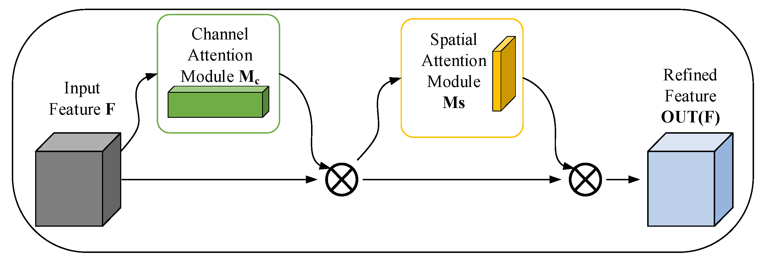
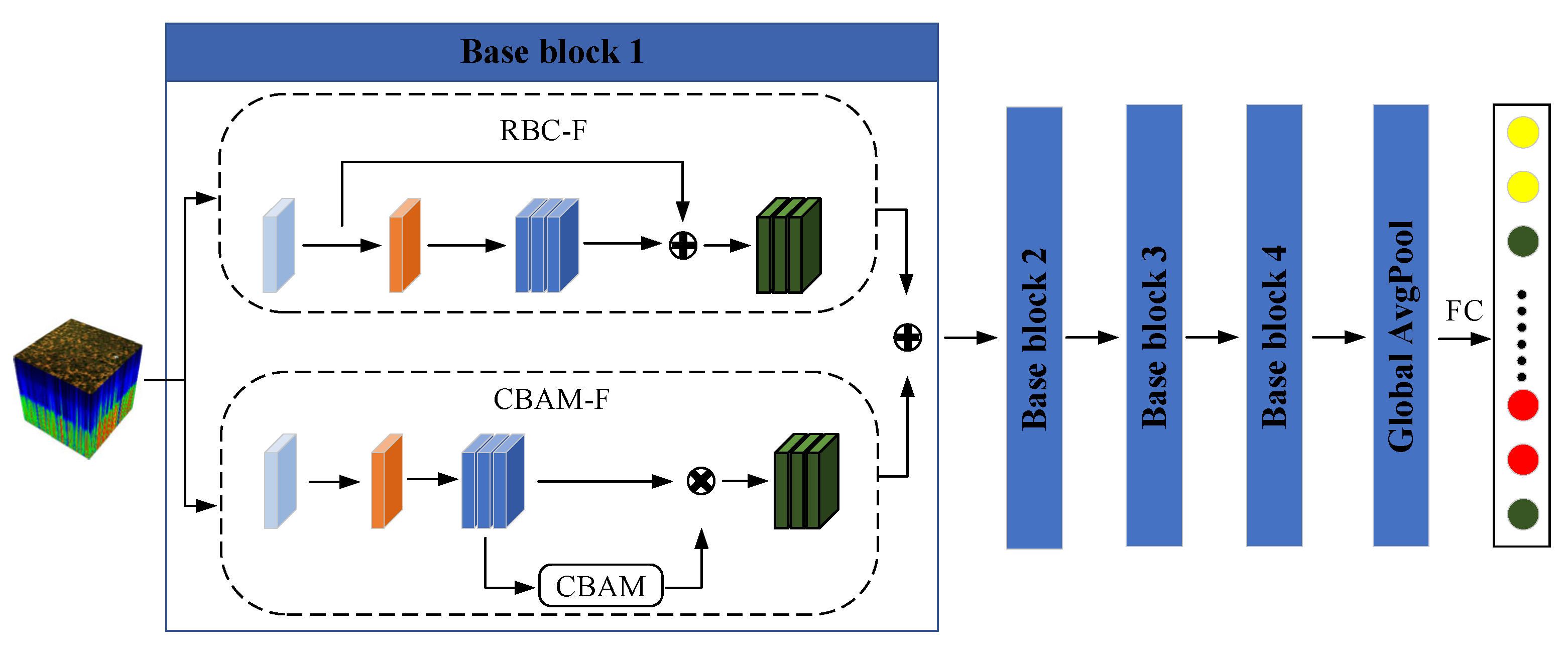
The model used improved convolutional block attention (CBAM-F) to effectively focus on important channel features and key spatial information and improved the model’s feature refinement capability by adaptively learning feature map channels and spatial relationships. It was combined with residual block convolution (RBC-F) to fuse the feature data and improve the model classification performance.

(3)

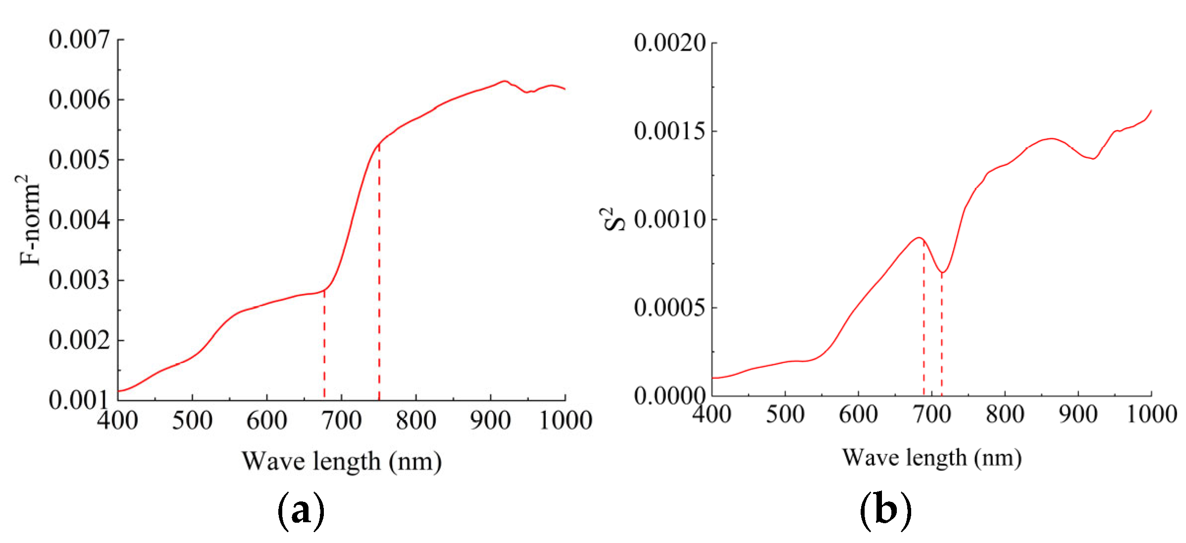
Using the variance and Frobenius norm² feature band selection methods, we could efficiently reduce the dimensionality of the data, enhance the computational efficiency of the model, retain important information for classification tasks, and effectively alleviate data redundancy in hyperspectral images.

2. Materials and Methods

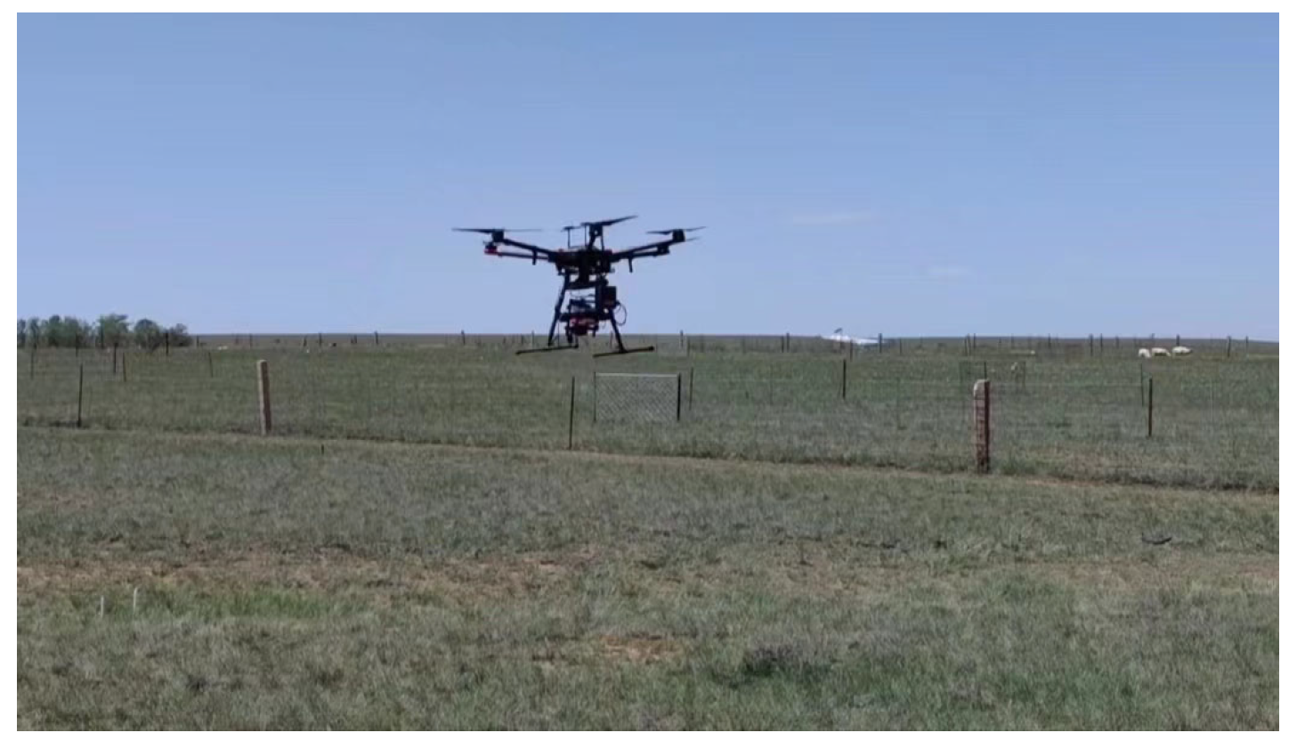
2.1. UAV Hyperspectral Remote Sensing System

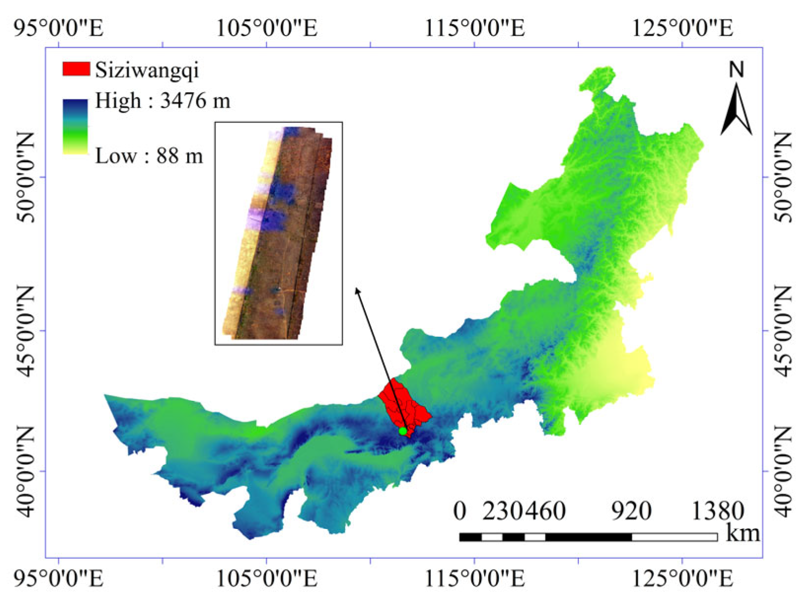
The system comprised a six-rotor UAV, hyperspectral imager, gimbal, onboard computer, handheld remote control, and battery. The hyperspectral imager used was the GaiaSky-mini hyperspectral imager developed by Shuangli Hopper, with 256 acquisition bands, a spectral range of 400–1000 nm, a spectral resolution of 3.5 nm, a hovering mode (built-in scanning), a lens focal length of 17 mm, and a lateral viewing angle of 29.6°. The drone was a DJI M600 Pro with a professional A3 flight control system, 9.5 kg empty, 6 kg maximum load, 16 min total load endurance, 4.5 kg maximum load, and ±0.02° angle jitter. The UAV hyperspectral remote sensing system is illustrated in Figure 1.

2.2. Study Area

The study area was situated in the Gegentara grassland of Siziwang Banner, Ulanqab City, Inner Mongolia Autonomous Region, China, with geographical coordinates of (41°75′36″ N,111°86′48″ E), as shown in Figure 2. The average altitude of the area is 1456 m, with an average annual precipitation of 280 mm. The temperature difference between day and night is substantial, and the average annual temperature ranges from approximately 1 to 6 °C. The area is crowded and falls under the Middle Temperate continental climate category. The soil type is light chestnut calcium soil with a high sand content. The grassland type is Stipa breviflora desert grassland, and the vegetation community type includes established species such as Stipa breviflora and dominant species such as Artemisia frigida.

2.3. Data Acquisition

Based on the grassland climatic conditions, vegetation growth cycles, sunlight intensity, and sun altitude variations, data were collected between 22 July and 31 July 2022, from 10:00 am to 2:00 pm. The weather was clear with no cloud cover, and the wind speed was less than level 3. The illumination type was natural light. The acquisition of single hyperspectral images was: 775 lines × 696 samples × 256 bands. Standard whiteboard corrections were performed before and after the UAV flight to prevent the overexposure or underexposure of the hyperspectral camera owing to changes in light intensity. During the experiment, a DJI Phantom 3 Pro UAV was used to acquire high-definition image data of the study area to provide an overview.

The experimental area covered 2.5 hectares. Given the low vegetation and sparse growth in the desert grassland, flying the UAV at an excessively high altitude would have resulted in a lower spatial resolution of the captured images, whereas an excessively low altitude would have limited the efficiency of the experiment. After the experimental investigation, the flight height of the UAV was set to 30 m and the spatial resolution of the image was 2.3 cm/pixel, which ensured experimental accuracy and simultaneously achieved the most suitable experimental effect. A total of 65 sampling plots were established with a sample size of 1 m × 1 m. Among them, there were 40 pure samples, 20 each of Stipa breviflora and Artemisia frigida, and 25 mixed samples with a size of 2 m × 2 m. For the hyperspectral image data acquisition, the type of plant taxa in the vegetation within each sample was recorded. The samples were marked with mats and small flags. The mixed samples were arranged according to the principle of uniform distribution. To ensure data reliability, each sample was photographed at least thrice.

2.4. Data Preprocessing

2.4.1. Feature Classification

During the UAV flight shooting, the hyperspectral images were distorted owing to the influence of external environmental factors. Therefore, a manual visual inspection method was used to remove such poorly imaged images. The remaining images were imported into the Spec-VIEW software for radiation correction so that the brightness values of the remote sensing image elements were converted into spectral reflectance. The corrected images were further screened for usable data using the ENVI 5.3 software. In the screened images, 100 pure image elements were extracted, including Artemisia frigida, Bare soil, Stipa breviflora, and others (mats and small flags). The spectral reflectance curves were plotted, as shown in Figure 3.

As shown in Figure 3, in the full wavelength range, the spectral reflectance curve of Feature 4 exhibited the strongest fluctuation and largest curve difference compared to the other features. One and three had prominent “peaks” and “troughs” in the spectral reflectance curve from 550 nm to 690 nm, but the difference in the reflectance fluctuation between them was more pronounced. The spectral reflectance curve of Feature 2 had a high growth rate and was similar to that of linear growth. These spectral reflectance fluctuation differences provide the potential for the fine classification of grassland features. The hyperspectral image data were cropped to 550 lines × 550 samples × 256 bands to facilitate data processing.

In Figure 3, 1 represents Artemisia frigida, 2 represents Bare soil, 3 represents Stipa breviflora, and 4 represents the others.

2.4.2. Data Labeling

In this study, 79,602 labels were produced using the ENVI 5.3 software by comparing the changes in the spectral reflectance curves of each pixel within the hyperspectral images and ground survey data.

Table 1. Label classification.

	Category	Number (N)
NO.	Name	Training	Validation	Testing
1	Artemisia frigida	9075	3870	13,003
2	Bare soil	13,785	5901	19,683
3	Stipa breviflora	4782	2079	6830
4	Other	218	91	285
5	Total	27,860	11,941	39,801

lists the specific label categories.

3. CNN Model Construction

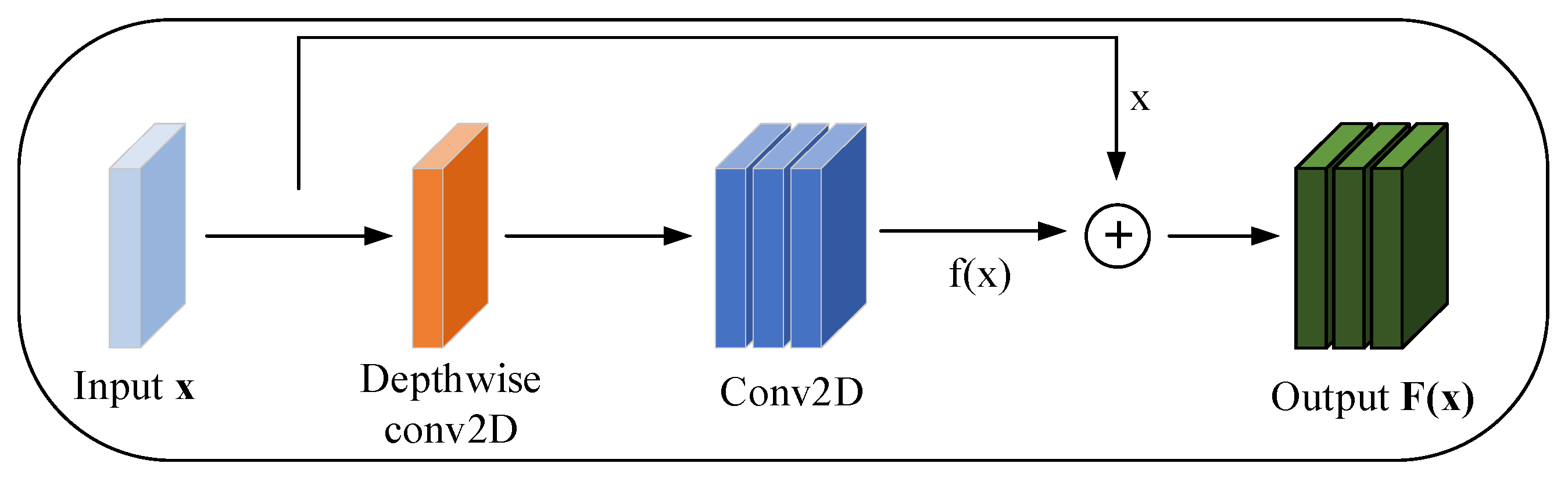
3.1. Improved Depth-Separable Convolution

The proposed network model used a convolutional approach based on Depthwise Separable Convolution (DSC). DSC was initially introduced into the MobileNet network model and comprises two components, that is, Depthwise Convolution (DW) and Pointwise Convolution (PW) [42]. In conventional convolution operations, the number of channels in each convolution kernel is the same as that in the input image, and a multichannel convolution operation is performed. However, in the DW convolution operation, the number of convolution kernels is the same as the number of channels in the input image, a single-channel convolution operation is performed, PW convolution is introduced, and 1 × 1 convolution kernels are used for the conventional convolution operation. To further improve the feature extraction capability, reduce the overfitting phenomenon, and prevent the gradient explosion problem, this model adds a Batch Normalization layer (BN) and ReLU activation function after the DW and PW convolution, respectively [43], to build an improved depth-separable convolution. Please refer to Equation (1) for the BN layer and Equation (2) for the ReLU activation function, respectively.

$$\{\begin{array}{c}{\mu }_B\leftarrow \frac{1}{m}{\displaystyle \sum _{i=1}^m{x}_i}\\ {\sigma }_B^2\leftarrow \frac{1}{m}{\displaystyle \sum _{i=1}^m{(x_i-{\mu }_B)}^2{x}_i}\\ \widehat{x_i}=(x_i-{\mu }_B)/\sqrt{{\sigma }_B^2+\epsilon }\\ y_i\leftarrow \gamma \widehat{x_i}+\beta \equiv B{N}_{\gamma ,\beta }(x_i)\end{array}$$

(1)

Equation (1), where: $x_i$ denotes the convolutional layer input, ${\mu }_B$ denotes the mean of a single factor, ${\sigma }_B^2$ denotes the variance of a single channel, $\widehat{x_i}$ denotes the normalization, $\gamma$ denotes the scaling factor, $\beta$ denotes the translation factor, and $y_i$ denotes the value normalized by introducing learnable parameters.

$$\mathrm{Re}lu(x)=\max \left(x,0\right)$$

(2)

Equation (2), where: $x$ represents the input value and $\mathrm{Re}lu(x)$ represents the model output.

3.2. Convolutional Block Attention Feature Refinement Module (CBAM-F)

In recent years, attention mechanisms have been widely used in deep learning owing to their ability to prioritize the most critical information in the input signal [44]. The CBAM is an end-to-end lightweight attention module, as shown in Figure 4. It consists of a Channel Attention Module (CAM) and Spatial Attention Module (SAM) and operates as follows:

$$OUT(F)=M_s(M_c(F)\otimes F)\otimes (M_c(F)\otimes F)$$

(3)

Equation (3), where $OUT(F)$ represents the model output, $F$ represents the model input, $M_c$ represents the channel attention, $M_s$ represents the spatial attention, and $\otimes$ represents congruent element multiplication.

The CBAM module enhances the classification performance of convolutional neural network models by focusing on the channel and spatial dimensions of the pixels and channels, which are crucial for image classification from CAM and SAM perspectives.

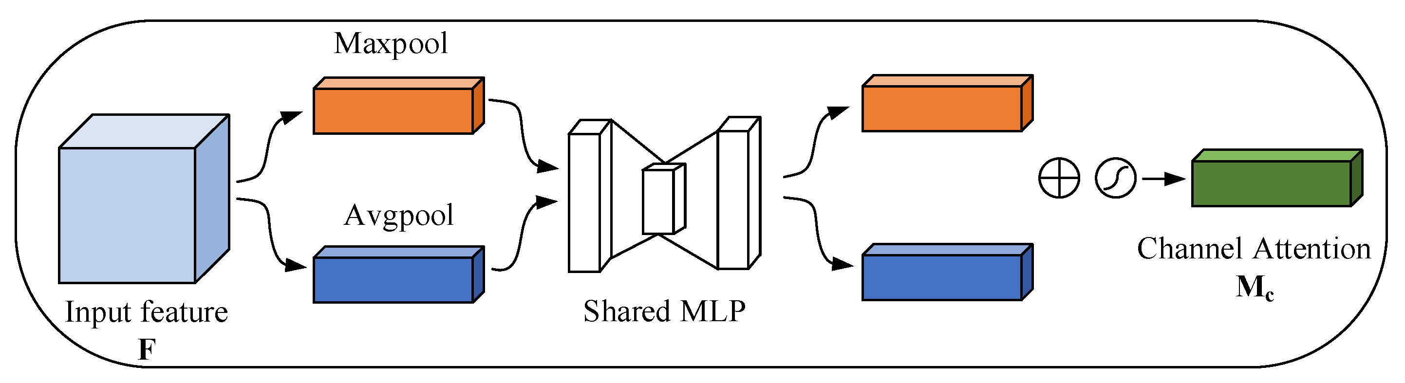
3.2.1. Channel Attention

The working principle of this system involves using the relationships between different channel features to produce channel attention maps, as shown in Figure 5. Two feature maps were generated by averaging the pooling layer and maximum pooling layer values across all channels, denoted as $F_{avg}^c\in R^{1\times 1\times c}$ and $F_{\max }^c\in R^{1\times 1\times c}$, respectively, where $c$ represents the number of channels. $F_{\mathrm{avg}}^c$ and $F_{\max }^c$ are then input into a shared feature network, that is, a multilayer perceptron (MLP). Their outputs are combined before being passed through a sigmoid activation function to generate the final channel attention map $M_c\in R^{1\times 1\times c}$.

This network model was inspired by the ECANet attention mechanism [45], which replaces the Shared MLP module in Figure 5 with a 2D-CNN convolution with a 1 × 1 kernel size. This approach prevents undesirable effects arising from a rapid reduction in dimensionality and improves inter-channel dependencies. Figure 6 illustrates this concept, and the mathematical formulation is provided in Equation (4).

$$\begin{array}{ll}{M}_c(F)& =\sigma (f^{1\times 1}(Avgpool(F^c))+f^{1\times 1}(Maxpool(F^c)))\\ & =\sigma (W_1(W_0(F_{avg}^c))+W_1(W_0(F_{\max }^c)))\end{array}$$

(4)

Equation (4), where: $\sigma$ is the sigmoid activation function; $f^{1\times 1}$ is a two-dimensional convolutional layer with a 1 × 1 convolutional kernel size; $F^c$ represents the model input; and $W_0,W_1$ is the MLP generation weight.

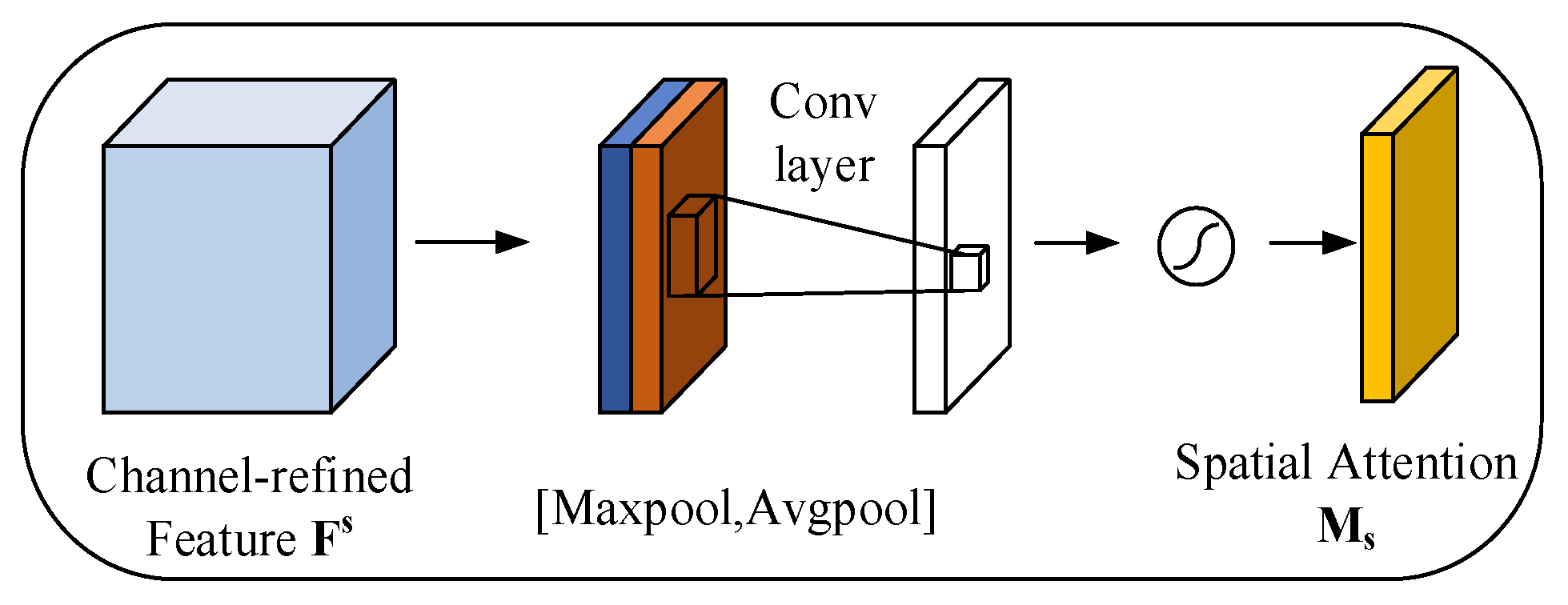
3.2.2. Spatial Attention

The working principle of this method is to generate spatial attention maps by using the spatial relationships between features (Figure 7). The average and maximum pooling layers were applied to the channel dimension to generate feature maps, denoted as $F_{avg}^s\in R^{H\times W\times 1}$ and $F_{\max }^s\in R^{H\times W\times 1}$, respectively. The two feature maps were then concatenated along the channel dimension and processed using a standard convolution operation with an output channel of 1, followed by a sigmoid activation function. This generated a spatial attention map known as $M_s\in R^{H\times W\times 1}$.

The mathematical equation is as (5) shown.

$$\begin{array}{ll}{M}_s(F)& =\sigma (f^{3\times 3}([Avgpool(F^s);Maxpool(F^s)]))\\ & =\sigma (f^{3\times 3}([F_{avg}^s;F_{\max }^s]))\end{array}$$

(5)

Equation (5), where: $\sigma$ is the sigmoid activation function, $f^{3\times 3}$ is a two-dimensional convolutional layer with a convolutional kernel size of 3 × 3, and $F^s$ is the model input.

3.3. Residual Block Convolution Feature Enhancement Module (RBC-F)

The primary purpose of this module is to reuse the underlying feature information through a residual structure, as shown in Figure 8. The output of the model component is modified by adding input x from the feature map of the upper layer, resulting in a change from the initial model output $f_{(x)}$ to $F_{(x)}$. If $f_{(x)}$ is equal to zero, the model becomes identity mapping. In this model, $f_{(x)}$ is obtained from an improved depth-separable convolution operation and the module is represented by Equation (6).

$$F(x)=f(x)+x$$

(6)

3.4. Streamlined 2D-CNN Model (SL-CNN)

The base block consisted of the CBAM-F and RBC-F modules. The SL-CNN model comprised four base blocks, a global average pooling layer (Global AvgPool), and a fully connected layer (FC), as shown in Figure 9. The model was run to the first base block, and the hyperspectral image was separately passed through two convolutional branches based on improved depth-separable convolution, so that the generated features were enhanced. The output results of the dual-branch channels were feature-fused to further enhance the generated features. Subsequently, the fused feature map was used as the input of the subsequent base block to continue the run downward. After four base block convolution operations, the model reached the global average pooling layer, where the input features were averaged to significantly reduce the model parameters and prevent overfitting. At the end of the model run, the output image feature map was passed through the FC layer, transforming the output from multidimensional to one-dimensional data. In addition, the FC layer served as a classification layer.

4. Results and Discussion

This experiment used the TensorFlow-GPU deep learning framework, Python programming language, Windows 10 as the operating system, NVIDIA RTX3060 with 6 GB of graphics, AMD R7-5800H as the CPU, and 16 GB of running memory. The model with the most successful performance in the validation set during the training was saved. The overall classification accuracy (OA), average accuracy (AA), single accuracy, test loss, and training time were used as evaluation metrics for model classification. The initial network parameters were set as follows: the sliding window size was 7 × 7; the loss function was the cross-entropy loss function; the optimizer was Adam; the initial learning rate was 0.001; the number of epochs was 50; and the batch size was 64. The hyperspectral images were downscaled to 51 bands using a PCA.

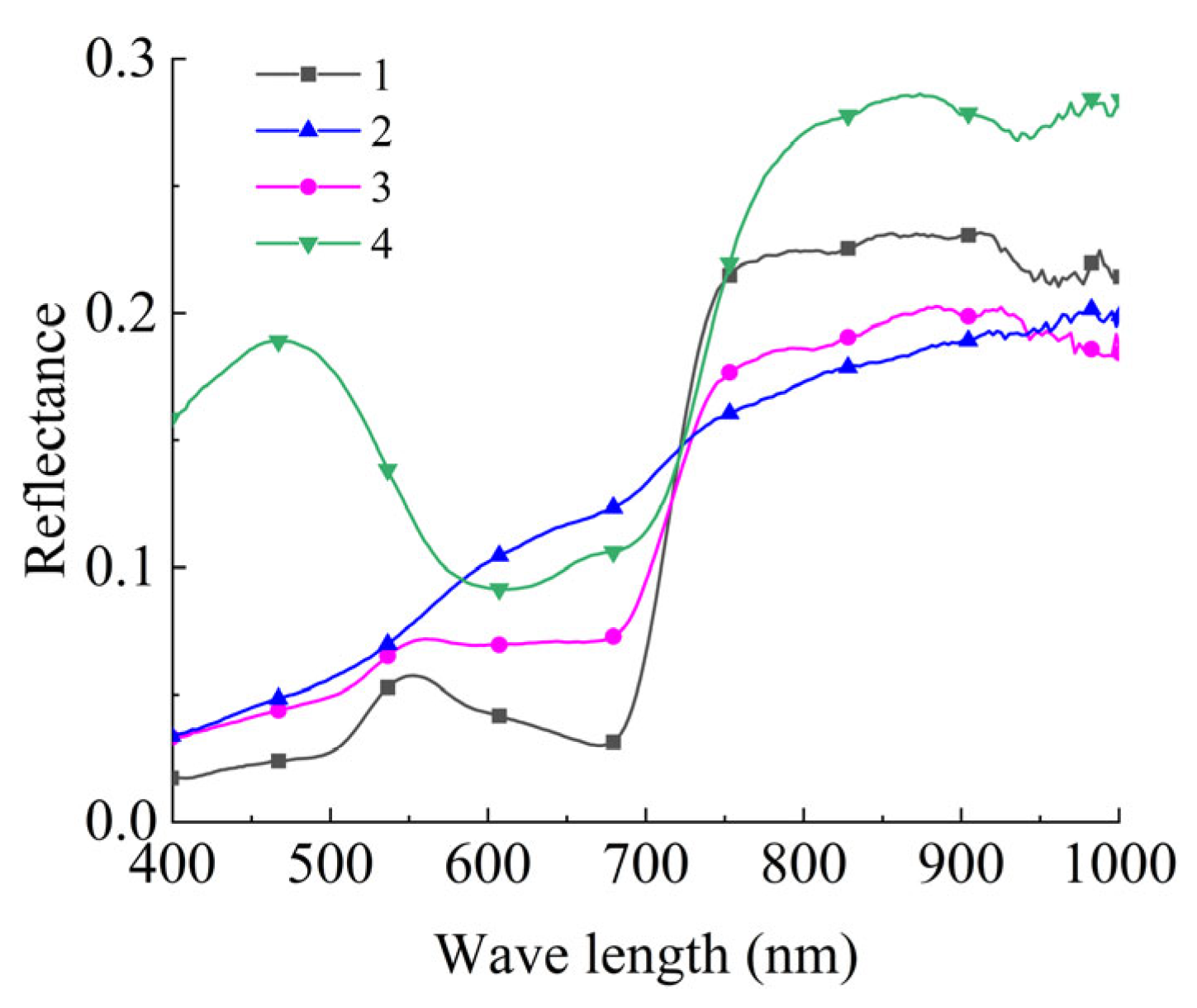
4.1. Waveband Processing

Hyperspectral image data contain hundreds of consecutive spectral bands that provide rich spectral and spatial information [46]. However, a higher number of bands leads to increased inter-band correlation, data redundancy, and computational costs, which can result in the Hughes phenomenon [47]. Therefore, reducing the dimensionality of data is necessary. However, the choice of dimensionality reduction method can affect the experimental results. In this experiment, the within-band variance-based combined with Frobenius norm² [48] (F-norm²) algorithm was compared with a principal component analysis (PCA), a standard dimensionality reduction algorithm for hyperspectral images, to select the most accurate classification result among the initial network model processing methods.

Variance [49] is typically used to describe the degree of deviation among data points in a random variable. F-norm² is used to describe the different distances between unrelated n-dimensional variables. In this experiment, the variance value for each spectral band was used to describe the degree of the dispersion of the information content among the spectral bands. The more significant the difference in variance values, the more dispersed the information. The F-norm² value describes the amount of information in each spectral band. The larger the F-norm² value, the richer is the information content. Equation (7) for calculating the variance is:

$$S^2(x)=\frac{{\displaystyle \sum _{i=1}^N{[x_i-\mu ]}^2}}{N}$$

(7)

Equation (7), where: $S^2(x)$ indicates the band variance, $N$ indicates the number of pixels in a single band, $x_i$ indicates the pixel value, and $\mu$ indicates the mean of the pixel values in a single band.

The F-norm² calculates the equation shown in (8):

$$\parallel X(:;:;\mathrm{b})\parallel F={({\displaystyle {\sum }_r^R{\displaystyle {\sum }_c^C|{X(r,c,b)|}^2}})}^{\frac{1}{2}}$$

(8)

Equation (8), where: $X$ is the tensor, $r$ is the number of rows (samples), $c$ is the number of columns (lines), and $b$ is the number of bands (bands).

Figure 10a schematically shows the normalized F-norm² values and Figure 10b the results of the within-band variance operation. Figure 10a shows that, before 677 nm (the number of bands is 96) and after 751 nm (166 band), although the number of bands increases further, the value decreases. In both cases, the number of intermediate bands was relatively small, but the value increased sharply. This indicated that the information content increased sharply at this time. In Figure 10b, there is a decline from 689 nm (126 band) to 713 nm (136 band), which is a turnaround compared to the bands before and after, indicating that the information in this band was relatively stable and concentrated. In summary, band division was conducted by choosing 126–136 bands as the center and the left and right bands as the increments. The experimental results are listed in

Table 2. Band selection table.

	Selection of Different Wave Numbers
Class	1	2	3	4	PCA	Full-band
Bands	126–136	116–146	106–156	96–166	11	256
Test loss (%)	0.022	0.023	0.024	0.020	0.026	0.051
Kappa × 100	98.735	98.637	98.617	98.788	98.524	96.858
OA (%)	99.216	99.156	99.143	99.249	99.085	98.053
Train time (s)	367	382	383	471	427	585

.

Table 2 shows that all four categories of bands achieved a better performance, and the training time increased with the increase in bands. The first and the fourth categories had a greater classification accuracy, but the overall accuracy difference was insignificant. Regarding time costs and the redundancy of the band information, the first category should be selected as the input band for the subsequent model. Under the same training conditions, the PCA dimensionality reduction method was used to select the first 11 principal components (the cumulative contribution rate of principal components was 99.10%) and the full-waveband image for training, respectively, and then they were compared with the results of the first category of runs, which showed that the results of the first category of runs had the best performance. In addition, an overall analysis of the results in Table 2 shows that the model using the full-band image operation had the longest training time and the lowest accuracy, and the model performance was poor, which also verifies the necessity of band selection for hyperspectral images. Therefore, 126–136 bands were selected as the model input bands.

4.2. Parameter Optimization

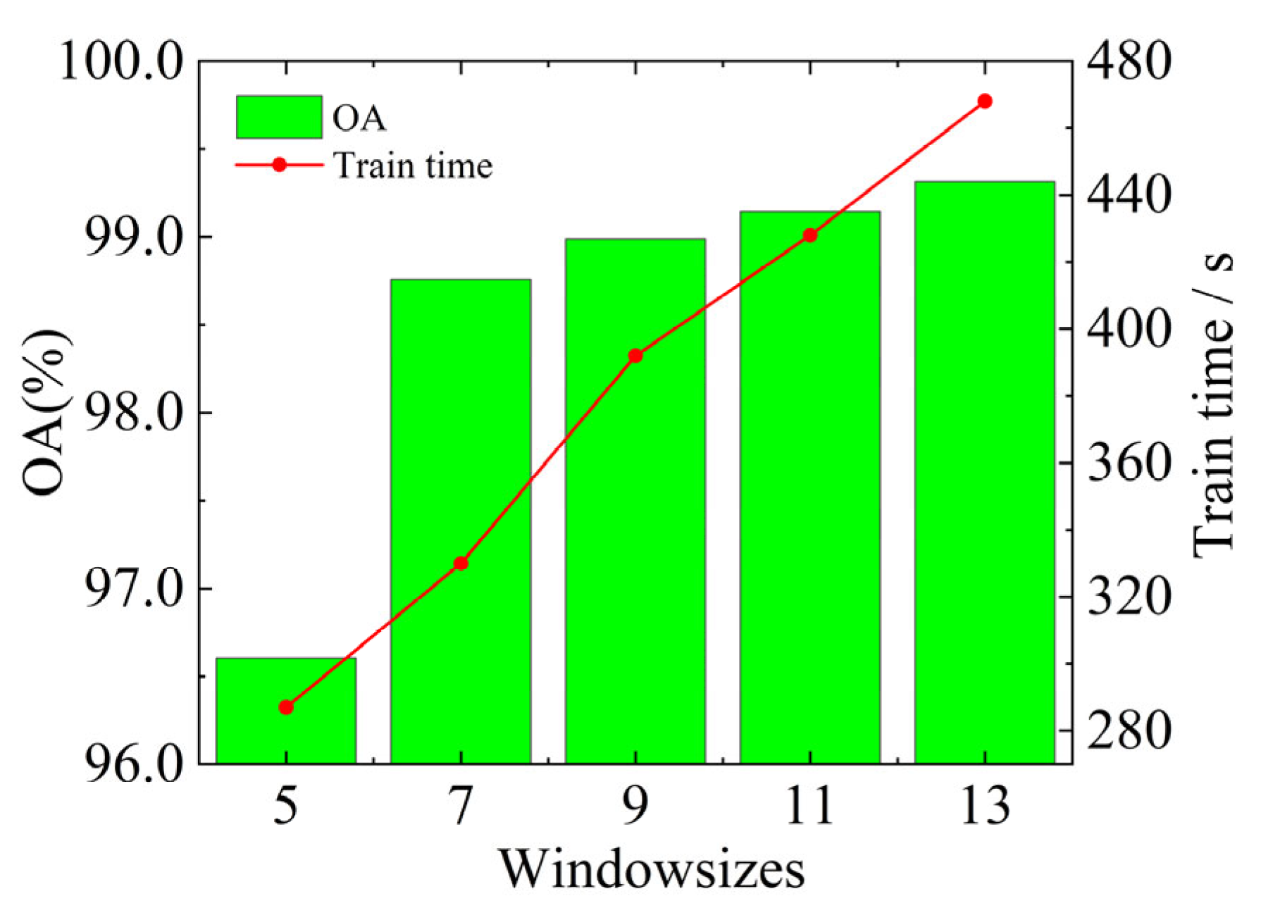
4.2.1. Window Size Selection

The larger the window size, the more information contained in the image texture, but there is also a greater information redundancy. To investigate the optimal window size for this model, five window sizes (5, 7, 9, 11, and 13) were used in the experiment. The results are presented in Figure 11. Figure 11 showed that, as the window size increased from left to right, both the model’s OA and training time values showed an increasing trend, but with different growth rates. However, when the window size was 11, the growth in both values was the smallest. The OA value was higher at 99.143% and the training time was 428 s. Therefore, for practicality, a window size of 11 was selected as the model input.

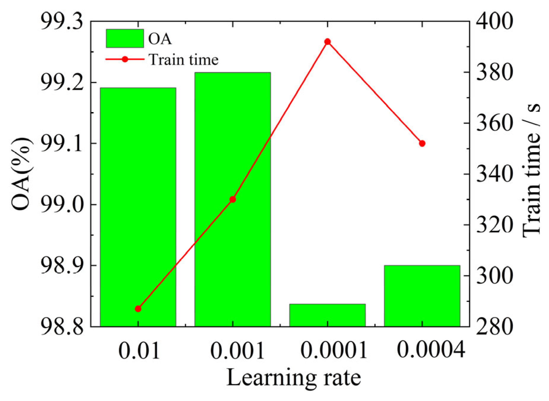
4.2.2. Learning Rate Selection

The learning rate is an essential factor that affects the speed of model construction. If it is set too large, the loss can explode; if it is set too small, it can lead to a slow loss reduction. Three sets of learning rates (0.01, 0.001, and 0.0001) were used to decrease the gradient and determine the most appropriate learning rate. To prevent the learning rate from decreasing too rapidly along the gradient, an additional group of learning rates (0.0004) was set for the control test. The experimental results are presented in Figure 12. Figure 12 shows that the model training time generally tended to increase and then decrease, and the overall classification accuracy reached its maximum when the learning rate was set to 0.001. Therefore, the learning rate for the model input was set as 0.001.

4.2.3. Batch Size Optimization

The batch size setting significantly affects the optimization of the constructed model and the memory usage of the computer. If the batch size is set too small, the gradient will be unstable, and it will be challenging for the model to converge. If the batch size is set too large, the speed of processing the same data will be accelerated, but the epoch required to achieve the same accuracy will also increase, and the model will quickly fall into a local optimum. Four different batch sizes (32, 64, 128, and 256) were compared, and the classification results are shown in Figure 13.

Figure 13 shows that, as the batch size increased, the overall classification accuracy and training time of the model gradually decreased. When the batch sizes were 32 and 64, respectively, the overall classification accuracy of the model performed well. Compared to the former, the overall classification accuracy decreased by 0.065% when the batch size was 64, but the training efficiency of the model increased by nearly 51.2%, which is in line with the demand from a practical point of view. Therefore, the batch size of the model input was selected to be 64.

4.2.4. Optimization of the Number of Base Blocks

After setting these parameters, we compared four different numbers of base blocks, that is, 2, 3, 4, and 5, to investigate their effects on this experiment. The classification performance results are listed in

Table 3. Comparison of the number of base blocks.

Base Block	2	3	4	5
OA (%)	98.188	98.912	99.216	99.342
Train time (s)	215	277	367	791
Memory (MB)	1.98	5.22	16.30	59.10
Model params (MB)	0.28	1.18	4.73	18.82

.

As shown in Table 3, the model results increased as the number of base blocks increased. The number of memory items and total parameters of the generated model increased at double or multiple rates. When the number of base blocks was four or five, the overall classification accuracy of the model was high, with the latter increasing by 0.126% compared with the former. However, the former only accounted for 46.40% and 27.58% of the latter in terms of the training time and memory used by the generated model, respectively. Therefore, we selected four base blocks as inputs for the model structure.

4.3. Comparison of Ablation Experiments

Ablation experiments were conducted to investigate the effectiveness of each module in the SL-CNN model. Five detailed evaluation metrics were selected, that is, overall accuracy (OA), average accuracy (AA), kappa, test loss, and mean F1 scores. The experimental results are listed in

Table 4. Comparison of ablation experiments.

RBC-F	CBAM-F	Kappa × 100	OA (%)	AA (%)	Test loss (%)	F1
✓		98.386	99.000	98.382	0.028	0.983
	✓	98.154	98.857	98.387	0.031	0.980
✓	✓	98.735	99.216	98.442	0.022	0.985

. As shown in the table, the SL-CNN model performed well in all aspects compared to a single module, particularly in the OA and Kappa terms, with improvements of 0.216% and 0.349, respectively, compared to the single RBC-F module. There were improvements of 0.359% and 0.581, respectively, compared to the single CBAM-F module. For the AA, test loss, and F1 score, the RBC-F and CBAM-F modules performed similarly when used alone in the model proposed in this study. However, both were inferior to the SL-CNN model with a combination of the two modules. Based on these results, the addition of both modules improved the classification performance of the model.

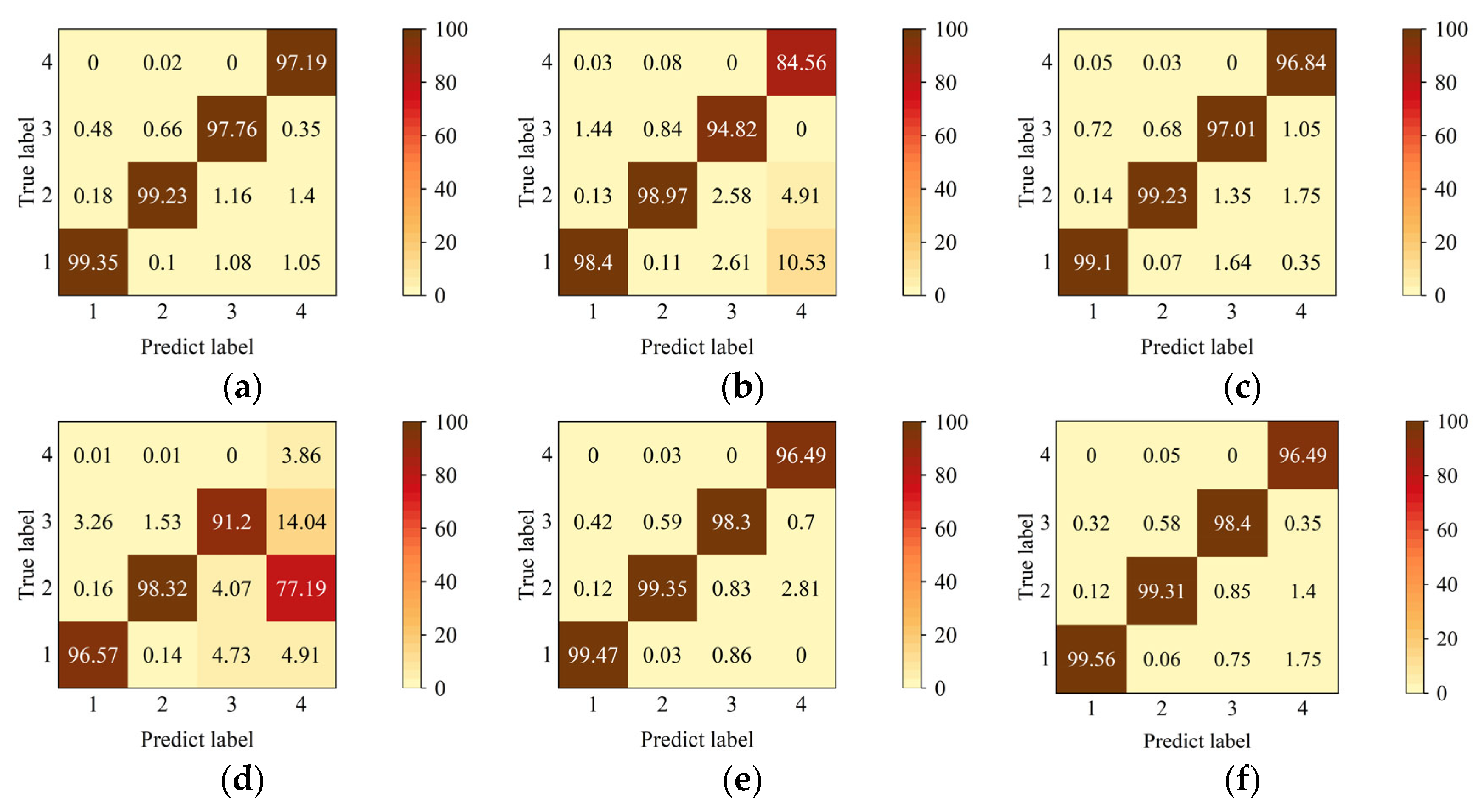
4.4. Experimental Results

The SL-CNN model continuously compared and optimized the initial network model structure and four operational parameters, resulting in further improvements in the performance and accuracy of the network model. For the hyperspectral images, after applying the band selection and model optimization techniques, the SL-CNN model achieved an increase of 0.46% in its overall accuracy (OA) compared to that of the initial model with the Windowsizes parameter set to 7, and there was a decrease of 61 s in the training time compared to that of the initial model with the Windowsizes parameter set to 11. Therefore, the band selection method and parameter optimization used in this study were confirmed to be beneficial for improving the classification performance of desert grassland hyperspectral images and accelerating the model construction.

To verify the validity of the SL-CNN model, four widely used hyperspectral model classification algorithms were selected for a comparative study that is, ResNet34, GoogLeNet, DenseNet121, and MLP. In addition, to verify the advantages of the improved depth-separable convolution, the conventional convolution method was used for reconvolution under the SL-CNN model to generate the 2D-CNN model. All the classification algorithms were executed in the same programming environment using the same data preprocessing method to ensure experimental reliability. The single-feature recognition classification accuracy results are shown in the confusion matrix (Figure 14).

Table 5. Comparison of different model classifications.

Class	ResNet34	GoogLeNet	DenseNet121	MLP	2D-CNN	SL-CNN
Kappa × 100	98.073	96.716	98.032	93.271	98.690	98.735
OA (%)	98.807	97.967	98.791	95.849	99.188	99.216
AA (%)	96.809	94.187	98.047	72.487	98.403	98.442
Train time (s)	2015	600	1491	25	557	367
Memory (MB)	247.0	93.4	92.2	21.7	55.8	16.3
Model params(MB)	81.38	28.76	27.02	7.21	17.91	4.73

presents the results.

As shown in Figure 14, the SL-CNN model constructed in this study had the most accurate overall performance, with recognition accuracies of 99.56%, 99.31%, 98.40%, and 96.49% for Features 1, 2, 3, and 4, respectively. This indicated that the SL-CNN model had a high capability for grassland feature extraction. As shown in Table 5, regarding the overall classification performance, the SL-CNN model achieved kappa coefficient, OA, and AA values of 98.735, 99.216%, and 98.442%, respectively. Its training time and generated model required the lowest memory compared to other models at 367 s and 16.3 MB, respectively, and the total number of parameters run during the model construction comprised 4.73 MB of the memory. The results showed that the SL-CNN had a high generalization ability and could be applied to desert grassland feature classification tasks.

4.5. Discussion

As shown in Figure 14 and Table 5, except for the Multilayer Perceptron (MLP) and GoogLeNet models, which had a poor recognition accuracy for Feature 4, all the other models achieved high recognition accuracies for the remaining features, with accuracies above 90%. ResNet34 was closer to the SL-CNN model regarding its single-feature recognition accuracy, but the other evaluation indices showed significant differences, in which the kappa coefficient, OA, and AA values were reduced by 0.662, 0.409%, and 1.633%, respectively, compared to the SL-CNN model. The ResNet34 model’s training time, the memory occupied by the generated model, and the number of total parameters of the model building run accounted for 18.21%, 6.60%, and 5.81% of the ResNet34 model, respectively. GoogLeNet had a high classification accuracy for Artemisia frigida and Bare Soil, but compared to the SL-CNN model, the classification accuracy of Feature 3 was significantly lower by 3.58%. Its generated model and the number of total parameters of the model building run, the memory occupied by the total number of parameters for the build run were 93.4 MB and 28.76 MB, respectively. This represented increases of 82.55% and 83.56% compared to the SL-CNN model. DenseNet121 had a single feature classification accuracy approximately similar to that of ResNet34 and possessed approximately the same memory occupation as GoogLeNet. However, the model training time was 72.487% that of ResNet34. The MLP had the lowest classification accuracy among all of the models, with an AA value of 72.487%. The detailed analysis results showed that the MLP is a fully connected network model with a simple model structure and limited feature extraction ability, resulting in the lowest classification accuracy for the fine features in desert grasslands. However, the model training time was shorter. In contrast, GoogLeNet used multiple parallel convolutional branches to capture grassland features at different scales and levels, which enhanced the model structure and network depth and improved the network expression ability. However, the model complexity was not high, and the features were not fully extracted, so the classification accuracy was limited. ResNet34 and DenseNet121 used a residual structure and dense connection structure, respectively. This increased the complexity and depth of the network, addressed the problems of gradient disappearance and information loss to the greatest extent, and improved the performance of fine-grained classification. However, they also introduced more operational parameters, which increased the model construction time and memory requirements. The SL-CNN model was different from the four conventional models mentioned above, especially ResNet34 and DenseNet121. It constructed the CBAM-F feature refinement module based on the improved depth-separable convolution by transforming the Shared MLP module in CBAM attention to 2D-CNN convolution. Additionally, SL-CNN also made full use of the residual structure to construct a residual block convolution feature enhancement module. These three elements synergized with each other to construct a lightweight design with a unique feature extraction capability, which allowed the SL-CNN model to significantly reduce the model parameters while maintaining high-precision image classification, effectively improving its memory efficiency and training speed. In summary, increasing the network depth, parallel structures, or using structures such as residuals is not fully applicable for desert grassland fine-grained feature classification, and the model structure should be optimized and adjusted appropriately.

The 2D-CNN and SL-CNN differed only in the convolution method. Therefore, the model classification accuracy was similar. However, the SL-CNN model’s training time, generated model, and the total number of parameters for the model building run accounted for 65.88%, 29.21%, and 26.41% of the memory of the 2D-CNN, respectively. This indicates that an improved depth-separable convolution is necessary for the convolutional approach.

In addition, we explored the differences between this model and other desertification-grassland feature classification models. In this study, the latest deep learning network models DIS-O [39], LGFEN [41], and GDIF-3D-CNN [50] for hyperspectral grassland feature recognition were selected for a comparative study. To ensure experimental reliability, the structure and parameters of the selected models were the same as those in the original study. The experimental results are listed in

Table 6. Comparison of the classification models of desert grassland features.

	GDIF-3D-CNN	DIS-O	LGFEN	SL-CNN
Kappa × 100	95.933	95.033	98.293	98.735
OA (%)	97.480	96.922	98.942	99.216
AA (%)	96.972	93.304	98.158	98.442
Train time (s)	49	63	233	367

. As shown in the table, all the models achieved more accurate results for the classification task. Although the SL-CNN model was not time efficient, it showed the highest accuracy in classification and consistency testing. This indicated that the SL-CNN model had an appropriate model complexity, could more effectively capture features, and had a stronger generalization ability and robustness. The DIS-O model had the lowest classification accuracy, mainly because of its relatively simple model structure, resulting in the extraction of grassland features. The DIS-O model had the lowest classification accuracy, mainly because of its relatively simple model structure, leading to an insufficient ability to extract grassland features. The DIS-O model was originally designed for a small number of classified species, and increasing the number of classified categories would lead to underfitting of the model and make its capacity insufficient. By replacing 2D convolution with 3D convolution, GDIF-3D-CNN improved the performance compared to the DIS-O model, indicating that 3D convolution helped to extract higher-level features. However, without further structural design, it still faces the problem of insufficient feature extraction capabilities. In contrast, the classification accuracy of the LGFEN model was slightly lower than that of the SL-CNN model, which indicates that the addition of the CBAM attention mechanism helped to improve the recognition and classification ability of desert grassland features and further enhanced the robustness of the model based on a separately designed feature extraction module.

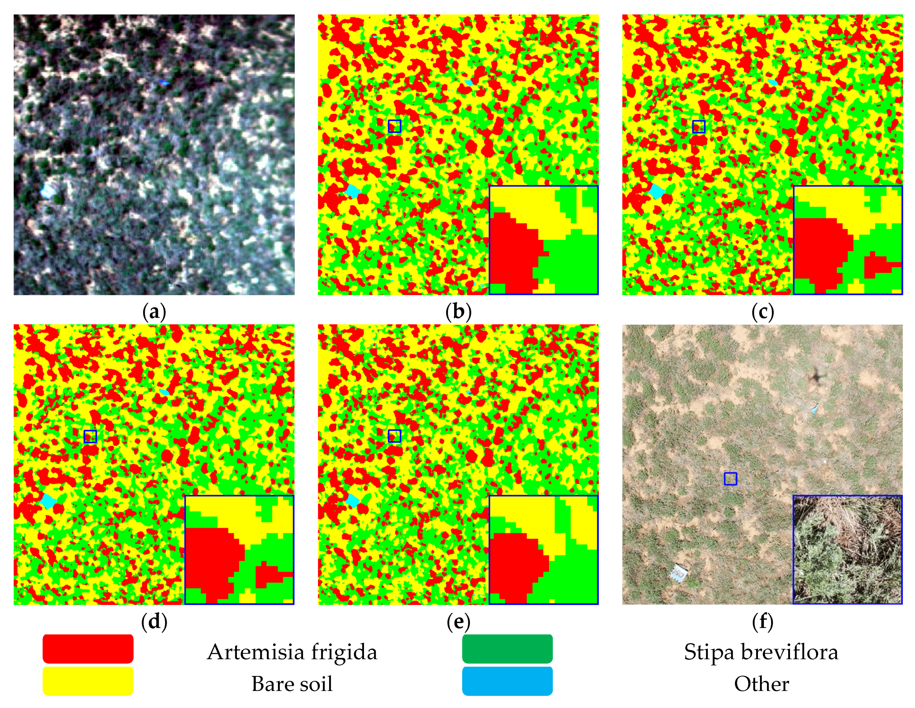
4.6. Data Visualization

A random set of sample data was selected for visualization and analysis to verify the optimized SL-CNN classification model and its practical classification performance. In addition, three grassland feature classification models, namely GDIF-3D-CNN, DIS-O, and LGFEN, were used to visualize the same samples for a comparative study. In the paper, to emphasize the real data on the ground after the model classification, the experimental markers (mats and small flags) part of the RGB color image captured by the DJI Phantom 3 Pro UAV was displayed, as shown in Figure 15f. The visualization and local zooming results of the classification of SL-CNN and the contrasting models are displayed in Figure 15b–e. After comparing the visualization results with ground survey data, the study’s results revealed that the DIS-O model had the worst overall classification performance, the GDIF-3D-CNN model had more pixel classification errors, and the LGFEN model misclassified more Stipa breviflora as Artemisia frigida. The predicted classification results of the SL-CNN model were the most consistent with the actual spatial distribution of the features and retained the spatial characteristics of the features effectively. This showed that the model had a high generalization ability and could meet the classification needs of desert grassland vegetation taxa.

While the primary focus of this study is on the desert grasslands of Inner Mongolia, its findings can offer fresh perspectives for ecological and environmental studies on a global scale. Additionally, the research could provide valuable theoretical references for similar studies conducted in other regions, signifying its significant contribution to understanding the functions of desert grassland ecosystems.

5. Conclusions

The classification of desert grassland taxa is essential for studying the process of grassland desertification. However, this study has some limitations. In this study, we built a UAV hyperspectral remote sensing system to collect remote sensing images of desert grassland vegetation efficiently and precisely under natural light to compensate for the shortcomings of traditional grassland survey methods. We developed a lightweight 2D-CNN model called SL-CNN for classifying desert grassland taxa. We used an improved depth-separable convolution to ensure species classification accuracy and achieve convenient and rapid species monitoring. To prevent information redundancy in the hyperspectral data, we used a combination of variance and F-norm² operations for feature band selection. We constructed a CBAM-F feature refinement module by improving the channel attention in the CBAM attention module. This was combined with the RBC-F residual block feature enhancement module to improve the feature extraction capability and classification performance of the network model.

In this study, four important parameters of the model were optimized, the effects of different parameter values on the classification performance of the model were analyzed, and ablation experiments were conducted to verify the effectiveness of the building blocks. To demonstrate the advantages of the model, it was compared with the latest and most commonly used hyperspectral image classification models. The results showed that the OA, AA, and Kappa values of this model performed more effectively than those of the other models, with 99.216%, 98.442%, and 98.735%, respectively. It had the advantages of fewer parameters, relatively fast construction, and lower memory occupation. This study has provided a new research method for monitoring the degradation of desert grassland features using UAV remote sensing technology.

However, desert grassland features are usually small and sparse, and the phenomenon of “same thing, different spectrum” and “same spectrum, different thing” often occurs in remote sensing images, which poses great difficulties in data annotation. Therefore, future research should address the effective classification and inversion of features using a small number of samples. In addition, the SL-CNN model needs to be further optimized to reduce its construction time and memory footprint for subsequent deployment in mobile terminals. This provides additional potential for practical applications.

References

1. Sun, J.; Ma, B.; Lu, X. Grazing enhances soil nutrient effects: Trade-offs between aboveground and belowground biomass in alpine grasslands of the Tibetan Plateau. Land Degrad. Dev. 2018, 29, 337–348. [Google Scholar] [CrossRef]
2. Zhang, Y.; Wang, L.; Yang, X.; Sun, Y.; Song, N. Sustainable application of GF-6 WFV satellite data in desert steppe: A village-scale grazing study in China. Front. Environ. Sci. 2023, 11, 57. [Google Scholar] [CrossRef]
3. Tsafack, N.; Fattorini, S.; Benavides Frias, C.; Xie, Y.; Wang, X.; Rebaudo, F. Competing vegetation structure indices for estimating spatial constrains in carabid abundance patterns in chinese grasslands reveal complex scale and habitat patterns. Insects 2020, 11, 249. [Google Scholar] [CrossRef] [PubMed]
4. Lv, G.; Xu, X.; Gao, C.; Yu, Z.; Wang, X.; Wang, C. Effects of grazing on total nitrogen and stable nitrogen isotopes of plants and soil in different types of grasslands in Inner Mongolia. Acta Prataculturae Sin. 2021, 30, 208–214. [Google Scholar]
5. Wang, M.; Zhang, C. Climate Change in Inner Mongolia Grassland and the Effects on Pastural Animal Husbandry. Grassl. Prataculture 2013, 25, 5–12. [Google Scholar]
6. Men, X.; Lv, S.; Hou, D.; Wang, Z.; Li, Z.; Han, G.; Sun, H.; Wang, B.; Wang, Z. Effects of grazing intensity on the density and spatial distribution of Cleistogenes songorica in desert steppe. Acta Agrestia Sin. 2022, 30, 3106–3112. [Google Scholar]
7. Dong, S.; Shang, Z.; Gao, J.; Boone, R.B. Enhancing sustainability of grassland ecosystems through ecological restoration and grazing management in an era of climate change on Qinghai-Tibetan Plateau. Agric. Ecosyst. Environ. 2020, 287, 106684. [Google Scholar] [CrossRef]
8. Fan, Y.; Li, X.-Y.; Li, L.; Wei, J.-Q.; Shi, F.-Z.; Yao, H.-Y.; Liu, L. Plant Harvesting Impacts on Soil Water Patterns and Phenology for Shrub-encroached Grassland. Water 2018, 10, 736. [Google Scholar] [CrossRef]
9. Guo, Q.; Hu, T.; Ma, Q.; Xu, K.; Yang, Q.; Sun, Q.; Li, Y.; Su, Y. Advances for the new remote sensing technology in ecosystem ecology research. Chin. J. Plant Ecol. 2020, 44, 418–435. [Google Scholar] [CrossRef]
10. Li, G.; Chen, C.; Li, J.; Peng, J. Advances in applying low-altitude unmanned aerial vehicle remote sensing in grassland ecological monitoring. Acta Ecol. Sin. 2023, 43, 6889–6901. [Google Scholar]
11. Li, C.; Han, W.; Peng, M. Improving the spatial and temporal estimating of daytime variation in maize net primary production using unmanned aerial vehicle-based remote sensing. Int. J. Appl. Earth Obs. Geoinf. 2021, 103, 102467. [Google Scholar] [CrossRef]
12. Lyu, X.; Li, X.; Dang, D.; Dou, H.; Wang, K.; Lou, A. Unmanned Aerial Vehicle (UAV) Remote Sensing in Grassland Ecosystem Monitoring: A Systematic Review. Remote Sens. 2022, 14, 1096. [Google Scholar] [CrossRef]
13. Daud, S.M.S.M.; Yusof, M.Y.P.M.; Heo, C.C.; Khoo, L.S.; Singh, M.K.C.; Mahmood, M.S.; Nawawi, H. Applications of drone in disaster management: A scoping review. Sci. Justice 2022, 62, 30–42. [Google Scholar] [CrossRef]
14. Yang, G.; Liu, J.; Zhao, C.; Li, Z.; Huang, Y.; Yu, H.; Xu, B.; Yang, X.; Zhu, D.; Zhang, X. Unmanned aerial vehicle remote sensing for field-based crop phenotyping: Current status and perspectives. Front. Plant Sci. 2017, 8, 1111. [Google Scholar] [CrossRef] [PubMed]
15. Lu, B.; Dao, P.D.; Liu, J.; He, Y.; Shang, J. Recent advances of hyperspectral imaging technology and applications in agriculture. Remote Sens. 2020, 12, 2659. [Google Scholar] [CrossRef]
16. Rueda-Ayala, V.P.; Peña, J.M.; Höglind, M.; Bengochea-Guevara, J.M.; Andújar, D. Comparing UAV-based technologies and RGB-D reconstruction methods for plant height and biomass monitoring on grass ley. Sensors 2019, 19, 535. [Google Scholar] [CrossRef] [PubMed]
17. Liu, E.; Zhao, H.; Zhang, S.; He, J.; Yang, X.; Xiao, X. Identification of plant species in an alpine steppe of Northern Tibet using close-range hyperspectral imagery. Ecol. Inform. 2021, 61, 101213. [Google Scholar] [CrossRef]
18. Wan, L.; Zhu, J.; Du, X.; Zhang, J.; Han, X.; Zhou, W.; Li, X.; Liu, J.; Liang, F.; He, Y. A model for phenotyping crop fractional vegetation cover using imagery from unmanned aerial vehicles. J. Exp. Bot. 2021, 72, 4691–4707. [Google Scholar] [CrossRef]
19. Sa, I.; Popović, M.; Khanna, R.; Chen, Z.; Lottes, P.; Liebisch, F.; Nieto, J.; Stachniss, C.; Walter, A.; Siegwart, R. WeedMap: A large-scale semantic weed mapping framework using aerial multispectral imaging and deep neural network for precision farming. Remote Sens. 2018, 10, 1423. [Google Scholar] [CrossRef]
20. Zhang, Y.; Ta, N.; Guo, S.; Chen, Q.; Zhao, L.; Li, F.; Chang, Q. Combining spectral and textural information from UAV RGB images for leaf area index monitoring in Kiwifruit Orchard. Remote Sens. 2022, 14, 1063. [Google Scholar] [CrossRef]
21. Yu, R.; Ren, L.; Luo, Y. Early detection of pine wilt disease in Pinus tabuliformis in North China using a field portable spectrometer and UAV-based hyperspectral imagery. For. Ecosyst. 2021, 8, 44. [Google Scholar] [CrossRef]
22. Hu, G.; Yao, P.; Wan, M.; Bao, W.; Zeng, W. Detection and classification of diseased pine trees with different levels of severity from UAV remote sensing images. Ecol. Inform. 2022, 72, 101844. [Google Scholar] [CrossRef]
23. Imran, H.A.; Gianelle, D.; Rocchini, D.; Dalponte, M.; Martín, M.P.; Sakowska, K.; Wohlfahrt, G.; Vescovo, L. VIS-NIR, Red-Edge and NIR-Shoulder Based Normalized Vegetation Indices Response to Co-Varying Leaf and Canopy Structural Traits in Heterogeneous Grasslands. Remote Sens. 2020, 12, 2254. [Google Scholar] [CrossRef]
24. Sun, G.; Jiao, Z.; Zhang, A.; Li, F.; Fu, H.; Li, Z. Hyperspectral image-based vegetation index (HSVI): A new vegetation index for urban ecological research. Int. J. Appl. Earth Obs. Geoinf. 2021, 103, 102529. [Google Scholar] [CrossRef]
25. Baloloy, A.B.; Blanco, A.C.; Ana, R.R.C.S.; Nadaoka, K. Development and application of a new mangrove vegetation index (MVI) for rapid and accurate mangrove mapping. ISPRS J. Photogramm. Remote Sens. 2020, 166, 95–117. [Google Scholar] [CrossRef]
26. Camps-Valls, G.; Campos-Taberner, M.; Moreno-Martínez, Á.; Walther, S.; Duveiller, G.; Cescatti, A.; Mahecha, M.D.; Muñoz-Marí, J.; García-Haro, F.J.; Guanter, L.; et al. A unified vegetation index for quantifying the terrestrial biosphere. Sci. Adv. 2021, 7, eabc7447. [Google Scholar] [CrossRef] [PubMed]
27. Xiao, L.; Yang, W.; Feng, M.; Sun, H.; Wang, C. Development of winter wheat yield estimation models based on hyperspectral vegetation indices. Chin. J. Ecol. 2022, 41, 1433–1440. [Google Scholar]
28. Jae-Hyun, R.; Jeong, H.; Cho, J. Performances of Vegetation Indices on Paddy Rice at Elevated Air Temperature, Heat Stress, and Herbicide Damage. Remote Sens. 2020, 12, 2654. [Google Scholar]
29. Wang, X.; Dong, J.; Baoyin, T.; Bao, Y. Estimation and Climate Factor Contribution of Aboveground Biomass in Inner Mongolia’s Typical/Desert Steppes. Sustainability 2019, 11, 6559. [Google Scholar] [CrossRef]
30. He, W.; Yu, L.; Yao, Y. Estimation of plant leaf chlorophyll content based on spectral index in karst areas. Guihaia 2022, 42, 914–926. [Google Scholar]
31. Pamungkas, S. Analysis Of Vegetation Index For Ndvi, Evi-2, And Savi For Mangrove Forest Density Using Google Earth Engine In Lembar Bay, Lombok Island. IOP Conference Series. Earth Environ. Sci. 2023, 1127, 012034. [Google Scholar] [CrossRef]
32. Umut, H.; NIJAT, K.; Chen, C.; Mamat, S. Estimation of Winter Wheat LAI Based on Multi-dimensional Hyperspectral Vegetation Indices. Trans. Chin. Soc. Agric. Mach. 2022, 53, 181–190. [Google Scholar]
33. Zhu, X.; Bi, Y.; Liu, H.; Pi, W.; Zhang, X.; Shao, Y. Study on the Identification Method of Rat Holes in Desert Grasslands Based on Hyperspectral Images. Chin. J. Soil Sci. 2020, 51, 263–268. [Google Scholar]
34. Yang, H.; Du, J.; Ruan, P.; Zhu, X.; LIiu, H.; Wang, Y. Vegetation Classification of Desert Steppe Based on Unmanned Aerial Vehicle Remote Sensing and Random Forest. Trans. Chin. Soc. Agric. Mach. 2021, 52, 186–194. [Google Scholar]
35. Zhang, S.; Gong, Y.; Wang, J. The Development of Deep Convolution Neural Network and Its Applications on Computer Vision. Chin. J. Comput. 2019, 42, 453–482. [Google Scholar]
36. Zhang, T.; Du, J.; Zhu, X.; Gao, X. Research on Grassland Rodent Infestation Monitoring Methods Based on Dense Residual Networks and Unmanned Aerial Vehicle Remote Sensing. J. Appl. Spectrosc. 2023, 89, 1220–1231. [Google Scholar] [CrossRef]
37. Pi, W.; Du, J.; Liu, H.; Zhu, X. Desertification glassland classification and three-dimensional convolution neural network model for identifying desert grassland landforms with unmanned aerial vehicle hyperspectral remote sensing images. J. Appl. Spectrosc. 2020, 87, 309–318. [Google Scholar] [CrossRef]
38. Wei, D.; Liu, K.; Xiao, C.; Sun, W.; Liu, W.; Liu, L.; Huang, X.; Feng, C. A Systematic Classification Method for Grassland Community Division Using China’s ZY1-02D Hyperspectral Observations. Remote Sens. 2022, 14, 3751. [Google Scholar] [CrossRef]
39. Zhu, X.; Bi, Y.; Du, J.; Gao, X.; Zhang, T.; Pi, W.; Zhang, Y.; Wang, Y.; Zhang, H. Research on deep learning method recognition and a classification model of grassland grass species based on unmanned aerial vehicle hyperspectral remote sensing. Grassl. Sci. 2023, 69, 3–11. [Google Scholar] [CrossRef]
40. Song, G.; Wang, Q. Species classification from hyperspectral leaf information using machine learning approaches. Ecol. Inform. 2023, 76, 102141. [Google Scholar] [CrossRef]
41. Zhang, T.; Bi, Y.; Du, J.; Zhu, X.; Gao, X. Classification of desert grassland species based on a local-global feature enhancement network and UAV hyperspectral remote sensing. Ecol. Inform. 2022, 72, 101852. [Google Scholar] [CrossRef]
42. Howard, A.G.; Zhu, M.; Chen, B.; Kalenichenko, D.; Wang, W.; Weyand, T.; Andreetto, M.; Adam, H. Mobilenets: Efficient convolutional neural networks for mobile vision applications. arXiv 2017, arXiv:1704.04861. [Google Scholar]
43. Ioffe, S.; Szegedy, C. Batch Normalization: Accelerating Deep Network Training by Reducing Internal Covariate Shift. Comput. Res. Repos. 2015, abs/1502.03167. [Google Scholar]
44. Fang, B.; Li, Y.; Zhang, H.; Chan, J.C.-W. Hyperspectral images classification based on dense convolutional networks with spectral-wise attention mechanism. Remote Sens. 2019, 11, 159. [Google Scholar] [CrossRef]
45. Han, G.; He, M.; Gao, M.; Yu, J.; Liu, K.; Liang, Q. Insulator Breakage Detection Based on Improved YOLOv5. Sustainability 2022, 14, 6066. [Google Scholar] [CrossRef]
46. Zhang, L.; Zhang, Q.; Du, B.; Huang, X.; Tang, Y.Y.; Tao, D. Simultaneous spectral-spatial feature selection and extraction for hyperspectral images. IEEE Trans. Cybern. 2016, 48, 16–28. [Google Scholar] [CrossRef]
47. Yuan, Y.; Zheng, X.; Lu, X. Discovering diverse subset for unsupervised hyperspectral band selection. IEEE Trans. Image Process. 2016, 26, 51–64. [Google Scholar] [CrossRef] [PubMed]
48. Wang, W.; Song, W.; Wang, G.; Zeng, G.; Tian, F. Image recovery and recognition: A combining method of matrix norm regularisation. IET Image Process. 2019, 13, 1246–1253. [Google Scholar] [CrossRef]
49. Fisher, R.A. XV.—The Correlation between Relatives on the Supposition of Mendelian Inheritance. Trans. R. Soc. Edinb. 2012, 52, 399–433. [Google Scholar] [CrossRef]
50. Pi, W.; Du, J.; Bi, Y.; Gao, X.; Zhu, X. 3D-CNN based UAV hyperspectral imagery for grassland degradation indicator ground object classification research. Ecol. Inform. 2021, 62, 101278. [Google Scholar] [CrossRef]
Figure 1. The UAV hyperspectral remote sensing system.
Applsci 13 12245 g001
Figure 2. Experimental area.
Applsci 13 12245 g002
Figure 3. Graph of reflectance of features.
Applsci 13 12245 g003
Figure 4. Convolutional block attention feature enhancement module.
Applsci 13 12245 g004
Figure 5. Channel attention.
Applsci 13 12245 g005
Figure 6. Improving channel attention.
Applsci 13 12245 g006
Figure 7. Spatial attention.
Applsci 13 12245 g007
Figure 8. Residual block convolution feature enhancement module.
Applsci 13 12245 g008
Figure 9. Streamlined 2D-CNN model.
Applsci 13 12245 g009
Figure 10. (a) F-norm2 operations and (b) variance operations.
Applsci 13 12245 g010
Figure 11. Window size comparison.
Applsci 13 12245 g011
Figure 12. Learning rates comparison.
Applsci 13 12245 g012
Figure 13. Batch size comparison.
Applsci 13 12245 g013
Figure 14. Comparison of confusion matrices for different models (a) ResNet34; (b) GoogLeNet; (c) DenseNet121; (d) MLP; (e) 2D-CNN; and (f) SL-CNN.
Applsci 13 12245 g014
Figure 15. Comparison of classification visualization results. (a) Original image; (b) SL-CNN; (c) LGFEN; (d) GDIF-3D-CNN; (e) DIS-O; and (f) RGB.
Applsci 13 12245 g015