Investigating the Nonlinear Effect of Built Environment Factors on Metro Station-Level Ridership under Optimal Pedestrian Catchment Areas via the Machine Learning Method

Abstract

Exploring the built environment factor’s impact on metro ridership can help develop metro station area planning strategies. This is in order to compensate for the shortcomings of previous studies, which mostly used all uniform pedestrian catchment areas (PCA) around metro stations. Beijing was divided into two zones and 12 built environment explanatory variables were selected as independent variables based on the “7D” dimension of the built environment. The boarding ridership during the morning peak hours was used as the dependent variable. Nineteen PCA radii from 200 to 2000 m were assumed. The optimal PCA of metro stations for each zone was determined by using the eXtreme Gradient Boosting (XGBoost) model with the objective of minimizing the Mean Absolute Percentage Error (MAPE). The nonlinear impact of the built environment factor of each zone on metro ridership is analyzed under the optimal PCA of metro stations. The study results show that (1) the optimal PCAs of metro stations inside the 4th Ring Road and outside the 4th Ring Road are the circular buffer zones with a radius of 800 m and 1300 m, respectively. (2) There is a nonlinear influence of the built environment factor on metro ridership, with strong threshold effects and spatial heterogeneity. The PCA results can be used for the built environment’s zoning of metro stations. The XGBoost model and the nonlinear impact results provide significant implications for the practice of station-level ridership forecasting and integrating TOD development and built environment renewal.

1. Introduction

The experience of some developed Western countries with high reliance on the car shows that car-based transport causes traffic congestion [1,2] and a range of environmental problems [3]. Metro transport is considered to be a better way of addressing the issues caused by high levels of car dependency [4,5,6] because it helps to reduce car dependency and congestion [7,8,9], improve road safety [10], and reduce social exclusion [11]. Therefore, urban policymakers highly value the construction and operation of metro transport [6,12], especially in developing countries [13]. The planning and construction of metro transport in China are rapidly growing. The 14th Five-Year Plan for the Development of a Modern Comprehensive Transport System issued by the State Council of the People’s Republic of China states that the total operational mileage of metro transport in the country will reach 10,000 km by 2025 [14]. However, mega-cities like Beijing have already experienced excessive ridership at some metro stations during peak morning hours. The urban metro operator in Beijing has had to limit the ridership to ensure the safety and comfort of metro operations [15]. Still, the measures to restrict the ridership have greatly affected the efficiency of residents’ travel. How to ensure that metro transport can meet the commuting needs of urban residents has become a widespread concern [16]. So, determining the factors influencing metro ridership is very important for the planning and operation of metro transport [2,4,17].

Linear models are widely used by scholars. However, linear models usually assume a linear function to fit the data. In real life, the influence of built environment factors may have a threshold effect. Therefore, using a linear model can cause errors in the results [18,19,20]. To date, Gradient Boosting Regression Tree (GBRT) models have been used to investigate the nonlinear influence of the built environment factor on metro ridership [3,21]. But, GBRT models suffer from over-fitting [19]. Daily and weekly ridership are widely focused and fewer have looked separately at peak-hour inbound or outbound ridership during the day. In addition, most existing studies have used experience, the TOD theory [22], or borrowed from others [23,24] to identify the pedestrian catchment areas (PCA) at metro stations, where most use a uniform size PCA of metro stations to calculate built environment factors.

Therefore, our study has three major purposes: (1) the optimal metro station PCA for the different zoning of Beijing’s metro stations was determined; (2) to investigate the nonlinear influence of the built environment of two zones on the ridership of the metro stations; (3) and to investigate the spatial heterogeneity of the nonlinear influence.

2. Literature Review

As an important public transport component, metro transport has received a great deal of scholarly attention in recent years [4,17,18,25]. Existing studies have found that the population density [26,27,28], density [17,29], accessibility [29,30], and land use mix [30] have an impact on subway ridership. This literature review focuses on four aspects of the research methodology, the determination of the PCA, the determination of dependent variables, and the determination of independent variables. The relevant transportation literature is summarized in Table 1.

In terms of research methods, the Ordinary Least Squares (OLS) model [4,16,31,32,33,34,35], Geographically Weighted Regression (GWR) model [23,36,37,38,39,40], structural equation models [31], and Multi-Scale Geographically Weighted Regression (MGWR) [17,22] model were used by a large number of scholars. These models can only examine the linear effect. However, some scholars have found that the effect of the built environment on metro passenger flow is nonlinear. [3,25]. With the boom in machine learning methods, random forests [41] and deep learning [42,43] have been applied to transportation. And, some scholars have used Gradient Boosting Regression Trees (GBRT) to analyze the nonlinear influence of the built environment on metro ridership [3,18,21,44]. However, the GBRT model has an overfitting problem [19]. The XGBoost model can accurately determine the nonlinear influence of independent variables on the dependent variable and it is also an excellent solution to the over-fitting problem [45]. In addition, XGBoost has the advantage of being extremely accurate and better at handling missing values and outliers [46,47]. XGBoost is currently being applied to predictive modeling [48,49,50,51], analysis of the residents’ travel behavior [19,52,53], factors triggering traffic accidents [54], and the impact of building configuration [55] on urban stormwater management. There are few studies using XGB to analyze the influence of the built environment on metro passenger flow.

Table 1. Summary of reference literature on transportation.

Author	Analysis Methods	Main Independent Variables	Dependent Variables	PCA	Travel Mode	Analysis Area
Estupiñán et al. (2008) [56]	Two Stage Least Square	socioeconomic characteristics	Daily ridership	250 m buffer zone	BRT	Bogotá, Columbia
Sohn et al. (2010) [31]	OLS/SEM	socioeconomic characteristics, accessibility, land use and density	Average weekday ridership	250 m buffer zone	Metro	Seoul, Republic of Korea
Loo et al. (2010) [35]	OLS	socioeconomic characteristics, accessibility, rail transit service	Average weekday ridership	N/A	Metro	New York, USA and Hong Kong, China
Gutiérrez et al. (2011) [33]	OLS	socioeconomic characteristics, land use and density	Monthly ridership	Threshold of change	Metro	Madrid, Spain
Sung et al. (2011) [34]	OLS	socioeconomic characteristics, accessibility	Ridership by time of day, week, and mode of transport	500 m buffer zone	Metro, Bus	Seoul, Republic of Korea
Cardozo et al. (2012) [36]	GWR/OLS	socioeconomic characteristics, accessibility	Monthly ridership	800 m and 200 m buffer zone	Metro	Madrid, Spain
Zhao et al. (2013) [4]	OLS	socioeconomic characteristics, accessibility, land use and density	Annual average weekday ridership	800 m buffer zone	Metro	Nanjing, China
Zhao et al. (2013) [16]	OLS	accessibility, rail transit service	Ridership between stations	800 m buffer zone	Metro	Nanjing, China
Hyungun et al. (2014) [1]	SER	land use and density, socioeconomic characteristics, rail transit service	Average weekday ridership	250, 500, 750, 1000, and 1500 m buffer zone	Metro	Seoul, Republic of Korea
Jun et al. (2015) [22]	MGWR	land use and density, socioeconomic characteristics		600 m buffer zone	Metro	Seoul, Republic of Korea
Calvo et al. (2019) [37]	GWR	land use and density, socioeconomic characteristics	Average weekday ridership	N/A	Metro	Madrid, Spain
Ding et al. (2019) [21]	Gradient Boosting regression trees (GBRT)	socioeconomic characteristics, accessibility, land use and density, rail transit service	Average inbound ridership on weekdays	400 m buffer zone	Metro	Washington, DC, USA
Li et al. (2020) [23]	GWR	land use and density, socioeconomic characteristics	Weekday ridership, weekend ridership, weekday morning peak arrivals and evening peak departures average, weekday morning peak departures and evening peak arrivals average	800 m buffer zone	Metro	Guangzhou, China
Gan et al. (2020) [3]	Gradient Boosting regression trees (GBRT)	socioeconomic characteristics, land use and density, rail transit service	OD ridership in different time periods of a day	800 m buffer zone	Metro	Nanjing, China
Andersson et al. (2021) [39]	GWR	“5D” of Built Environment	Seasonal daily traffic volume	600 m buffer zone	Metro	Tai Pei, China
Wang et al. (2022) [17]	MGWR	“7D” of Built Environment	Alighting ridership during the morning peak hours	Overlapped by 1000 m radius circular buffer zone and Thiessen polygon	Metro	Beijing, China
Du et al. (2022) [18]	Gradient Boosting regression trees (GBRT)	socioeconomic characteristics, land use and density, rail transit service	Weekday daily ridership, weekend ridership, weekday morning peak ridership, weekday evening peak ridership	800 m grid distance	Metro	Xian, China

Table 1. Summary of reference literature on transportation.

Author	Analysis Methods	Main Independent Variables	Dependent Variables	PCA	Travel Mode	Analysis Area
Estupiñán et al. (2008) [56]	Two Stage Least Square	socioeconomic characteristics	Daily ridership	250 m buffer zone	BRT	Bogotá, Columbia
Sohn et al. (2010) [31]	OLS/SEM	socioeconomic characteristics, accessibility, land use and density	Average weekday ridership	250 m buffer zone	Metro	Seoul, Republic of Korea
Loo et al. (2010) [35]	OLS	socioeconomic characteristics, accessibility, rail transit service	Average weekday ridership	N/A	Metro	New York, USA and Hong Kong, China
Gutiérrez et al. (2011) [33]	OLS	socioeconomic characteristics, land use and density	Monthly ridership	Threshold of change	Metro	Madrid, Spain
Sung et al. (2011) [34]	OLS	socioeconomic characteristics, accessibility	Ridership by time of day, week, and mode of transport	500 m buffer zone	Metro, Bus	Seoul, Republic of Korea
Cardozo et al. (2012) [36]	GWR/OLS	socioeconomic characteristics, accessibility	Monthly ridership	800 m and 200 m buffer zone	Metro	Madrid, Spain
Zhao et al. (2013) [4]	OLS	socioeconomic characteristics, accessibility, land use and density	Annual average weekday ridership	800 m buffer zone	Metro	Nanjing, China
Zhao et al. (2013) [16]	OLS	accessibility, rail transit service	Ridership between stations	800 m buffer zone	Metro	Nanjing, China
Hyungun et al. (2014) [1]	SER	land use and density, socioeconomic characteristics, rail transit service	Average weekday ridership	250, 500, 750, 1000, and 1500 m buffer zone	Metro	Seoul, Republic of Korea
Jun et al. (2015) [22]	MGWR	land use and density, socioeconomic characteristics		600 m buffer zone	Metro	Seoul, Republic of Korea
Calvo et al. (2019) [37]	GWR	land use and density, socioeconomic characteristics	Average weekday ridership	N/A	Metro	Madrid, Spain
Ding et al. (2019) [21]	Gradient Boosting regression trees (GBRT)	socioeconomic characteristics, accessibility, land use and density, rail transit service	Average inbound ridership on weekdays	400 m buffer zone	Metro	Washington, DC, USA
Li et al. (2020) [23]	GWR	land use and density, socioeconomic characteristics	Weekday ridership, weekend ridership, weekday morning peak arrivals and evening peak departures average, weekday morning peak departures and evening peak arrivals average	800 m buffer zone	Metro	Guangzhou, China
Gan et al. (2020) [3]	Gradient Boosting regression trees (GBRT)	socioeconomic characteristics, land use and density, rail transit service	OD ridership in different time periods of a day	800 m buffer zone	Metro	Nanjing, China
Andersson et al. (2021) [39]	GWR	“5D” of Built Environment	Seasonal daily traffic volume	600 m buffer zone	Metro	Tai Pei, China
Wang et al. (2022) [17]	MGWR	“7D” of Built Environment	Alighting ridership during the morning peak hours	Overlapped by 1000 m radius circular buffer zone and Thiessen polygon	Metro	Beijing, China
Du et al. (2022) [18]	Gradient Boosting regression trees (GBRT)	socioeconomic characteristics, land use and density, rail transit service	Weekday daily ridership, weekend ridership, weekday morning peak ridership, weekday evening peak ridership	800 m grid distance	Metro	Xian, China

Determining the PCA for a metro station is considered very important before conducting research [17]. Currently, most studies use circular buffers [1,4,16,22,23,31,34,36,52,56] centered on the metro station as the PCA. However, considering that the station study areas overlap in areas with a dense distribution of metro stations, Tyson polygons [57] or Tyson polygons superimposed with circular buffers to take the intersection [17,23,24] have been used to determine the PCA. The radii of circular buffers chosen by different scholars varied widely, with more scholars choosing a circular buffer radii of 400 m [21], 500 m [31,34], 600 m [22,39,52], 800 m [3,4,16,23,36], and 1000 m [1,17]. In addition, the choice of buffer radius mostly relies on pedestrian accessibility [22,32,36], experience [4], and drawing on the research of others [23]. Existing research has shown that the PCA for metro stations varies from city to city (57) and that one cannot borrow the PCA for metro stations in other cities. Thus, the PCA of metro stations has been determined using the goodness of fit of regression models [17,39]. Although some scholars have found the PCA via regression fit superiority methods, they tend to use a single PCA of metro stations. And, with the rapid development of cities, mega-cities like Beijing are establishing new districts on the outskirts of the city, which tend to be larger in scale. Therefore, using the uniform PCA of metro stations would make the error of the model larger. Although, scholars have already divided the city into three zones [39]. But, this study still uses a uniform PCA of metro stations across the three zones. To our knowledge, no scholars have identified separate metro station’s PCA according to different zones.

In terms of the selection of dependent variables, daily ridership was the most popular among scholars [1,4,21,31,33,34,35,36,37,56], while some other scholars chose monthly ridership [33,36] and seasonal ridership [39] as dependent variables. In addition, some scholars will choose several dependent variables in one article [18,23,34]. Fewer scholars consider boarding or alighting ridership during the morning peak hours on the working day alone. But, the fact is that for mega-cities like Beijing, the morning rush hour is the time of most significant conflict, and there are already morning rush hour entry restrictions at metro stations. We think that a separate analysis of boarding ridership during the morning peak hours is important to improve metro operations’ efficiency and adjust metro station traffic later. Fewer academics have analyzed the boarding ridership during the morning peak hours separately.

In terms of the selection of explanatory variables, the main explanatory variables in the existing studies include land use and density [1,4,16,22,23,31,33,37,58], socioeconomic characteristics [4,22,31,33,34,35,36,37,56,58], accessibility [1,4,16,31,32,34,35,36,37,58], and metro service (including metro service level and metro service quality) [32,35,37]. However, there is a lack of systematic selection of explanatory variables. Therefore, scholars have systematically selected the explanatory variables based on the “5D” dimension [59]. However, there is a lack of population-related explanatory variables in the “5D” dimension. Scholars add demand management and demographics to the “5D” dimension, thus introducing the “7D” dimensions [60]. The “7D” dimension has been used in studies [17].

This study focuses on the impact of the “7D” built environment on the boarding ridership during the morning peak hours. The XGBoostwas was used to determine the optimal PCA for different zones. And, the nonlinear influence of the built environment on subway passenger flow and its spatial heterogeneity are studied under an optimal subway PCA.

3. Study Scope and Data

3.1. Study Scope and Data Sources

The study was carried out on a total of 292 metro stations that are already in service on 19 lines in Beijing in 2020. We find that the distribution of metro stations inside the 4th Ring Road is more concentrated, while the distribution of metro stations outside the 4th Ring Road is more dispersed. So, all metro stations in Beijing are divided into two zones: metro stations inside the Fourth Ring Road (white-filled areas) and metro stations outside the Fourth Ring Road (yellow-filled areas) (Figure 1). The data source of the dependent variable is the Beijing public transport IC card data. We obtained the average hourly inbound passenger flow of Beijing’s metro stations during the five working days of the week from 12 October 2020 to 16 October 2020. Based on the trend of boarding ridership (Figure 2), the morning peak of Beijing’s metro transit is 7:00–9:00. Considering that the contradiction is more prominent in the morning peak hour and the space is limited, this paper only analyzes the boarding ridership during the morning peak hours (hereafter referred to as metro ridership). Figure 1 also shows the spatial distribution of passenger flow at the station level in Beijing.

3.2. Explanatory Variables of the Built Environment

The “7D” dimensions were constructed by adding demand management and demographic factors to the built environment’s “5D” dimensions [59]. It consists of seven sections: density, diversity, design, destination accessibility, distance, demand management, and demographics. [60]. It has been proved that the number of POI has an impact on metro ridership [61,62]. Therefore, the density of POIs is changed to the number of POIs in the study. The built environment dataset was constructed on this basis and included 12 built environment explanatory variables(

Table 2. Explanatory variables.

Built Environment Category	Interfering Factor	Unit
Density	Building density	m2/km2
Diversity	Mixed utilization of land
Design	Road density	km/km2
	Floor area ratio
Destination accessibility	Number of entrances and exits	quantity
	Number of commercial facilities
	Number of office facilities
	Number of public service facilities
Distance to transit	Density of bus lines	km/km2
Demand management	Number of parking lots	quantity
	Number of bus stops
Demographics	Population	quantity

). For the data sources and the calculation methods of the explanatory variables, see other research results of our research group [17].

4. Methods

4.1. Pedestrian Catchment Areas (PCA) Delineation for Metro Stations

A key task before analyzing the nonlinear influence of the built environment factor on ridership at metro stations is how to define the scope of the built environment analysis for metro stations [30]. The extent of the built environment analysis for metro stations is determined using the “maximum” walking distance or the area within walking distance of most users [4,63]. For this reason, a metro station’s built environment analysis area is often referred to as pedestrian catchment areas (PCA). In existing studies, the PCA of metro stations varies widely, from a minimum of 250 m [1,56] to a maximum of 1500 m. In order to more accurately determine the PCA of the metro stations in the two zones of Beijing, the circular buffer zones with a radius of 200–2000 m (interval 100 m) is selected as the PCA of metro stations in the two zones, respectively. The minimum of Mean Absolute Percentage Errors (MAPE) of the XGBoost models under multiple PCAs were used to determine the optimal PCA for the two zones of metro stations.

4.2. eXtreme Gradient Boosting (XGBoost)

XGBoost is an improved algorithm based on gradient-augmented decision trees, proposed by Chen et al. in 2016 [46]. The XGBoost model is not only an excellent solution to the overfitting problem. It also has the advantages of high accuracy and better handling of missing values and outliers [46,47]. The regression function of XGBoost usually consists of two parts: training loss and regularization. Its objective function expression is:

$$Obj\left(\mathsf{\Phi }\right)=L\left(\mathsf{\Phi }\right)+\mathsf{\Omega }\left(\mathsf{\Phi }\right)$$

(1)

where L is the training loss function, and Ω is the regularization term. The training loss is used to measure the performance of the model on the training data. The purpose of the regularization term is to control the complexity of the model, and the over-fitting of the model can be controlled by the regularization term [64]. In this study, the training set is 70% of the total data, and the test set is 30% of the total data. The parameter configuration of the XGBoost model we selected for this study is shown in

Table 3. The parameter configuration of the XGBoost model.

Parameter	Implication	Value
max_depth	Maximum tree depth, which controls the model complexity, can be used to prevent overfitting	8
eta	The learning rate, which controls the weights of each step of the fitting process, can be used to improve the model accuracy	0.20
subsample	Random sampling ratio, which controls the proportion of random samples per tree, can be used to prevent overfitting	0.75
colsample_bytree	The column sampling rate represents the column fraction of a random sample of each tree	0.80
n_estimators	Return the number of trees	461
gamma	The leaf node split threshold, which specifies the minimum loss reduction that must occur for splitting	0.20

.

4.3. Explanation of Machine Learning Models: SHAP (Shapley Additive exPlanations)

SHAP (Shapley Additive exPlanations) is used to explain the machine learning models and was proposed by Lundberg and Lee in 2021 [65]. The formula for calculating the SHAP value is expressed as:

$${\theta }_i={\displaystyle \sum _{S\in N\backslash \left\{i\right\}}\frac{\left|S\right|!\left(\left|F\right|-\left|S\right|-1\right)!}{\left|F\right|!}}\left[f_{S\cup \left\{i\right\}}\left(X_{S\cup \left\{i\right\}}\right)-f_S\left(X_s\right)\right]$$

(2)

where i denotes a feature. F is the set of features containing all features. S is the set of all features without feature i. $\left|S\right|!$ is the factorial of the number of features contained in S. $X_s$ is the input feature values in S. $f_{S\cup \left\{i\right\}}$ is a model trained with feature i. $f_S$ is another model trained without feature i. $\left[f_{S\cup \left\{i\right\}}\left(X_{S\cup \left\{i\right\}}\right)-f_S\left(X_s\right)\right]$ is the difference between the outputs of the two models.

4.4. Mean Absolute Percentage Error

The Mean Absolute Percentage Error (MAPE) is a measure of a relative error that uses absolute values to avoid positive and negative errors canceling each other out. The MAPE has been found to be a more accurate determination of the model’s accuracy [66], with smaller MAPE values proving that the model is more accurate. The formula for calculating the MAPE is expressed as:

$$\mathrm{MAPE}=\frac{100\%}{n}{\displaystyle \sum _{i=1}^n\left|\frac{{\widehat{y}}_i-y_i}{y_i}\right|}$$

(3)

where n is the total number of metro stations. ${\widehat{y}}_i$ is the predicted value of the explanatory variable for the ith orbital site. y_i is the actual value of the explanatory variable for the ith orbital site.

5. Results and Discussion

5.1. Optimal Metro Stations PCA for Different Zones

In order to determine the rationality of the XGBoost model in this analysis, we compared the accuracy of the XGBoost model with other machine learning models and the comparison results of AdjR² are shown in Figure 3. As can be seen from Figure 3, the accuracy of the XGBoost model is better than others, and the AdjR² of the testing set inside the 4th Ring Road is 0.74 and the AdjR² of the testing set outside the 4th Ring Road is 0.72. So, XGBoost can be used for this analysis. Calculate the MAPE of PCAs for the inside and outside 4th Ring Road metro stations based on the predicted values in the XGBoost model in the testing set and the true values in the testing set, respectively, and plot the line graph of MAPE at different PCAs. To our knowledge, the accuracy of nonlinear models has not been considered in previous studies. In addition, most scholars currently studying the nonlinear influence of the built environment factor on metro ridership have used the goodness of fit for linear models [17,39] and experience [3,18,21] to determine the optimal PCA of metro stations. No one has used the accuracy of nonlinear models to determine the optimal PCA of metro stations. Figure 4 shows the MAPE folds at different PCAs of metro stations inside and outside the 4th Ring Road. The graph shows that when the buffer zone radius is 800 m, the lowest MAPE value is reached at 9.64% for metro stations inside the 4th Ring Road. Therefore, the optimal PCA of metro stations inside the 4th Ring Road is the circular buffer zone of an 800 m radius. For the outside 4th Ring Road metro stations, MAPE reaches a minimum value of 16.60% when the buffer radius is 1300 m. So, the optimal PCA of the outside 4th Ring Road metro stations is a circular buffer of 1300 m.

Looking at the MAPEs of the metro stations inside and outside the 4th Ring Road, the MAPE of the metro stations outside the 4th Ring Road is larger than those of the metro stations inside the 4th Ring Road. It proves that the model accuracy is higher inside the 4th Ring Road. That is consistent with existing research [39]. This is due to the fact that outside the 4th Ring Road is a new urban area with a larger urban scale. Some passengers do not start their journey in the PCA but still choose to come to this metro station.

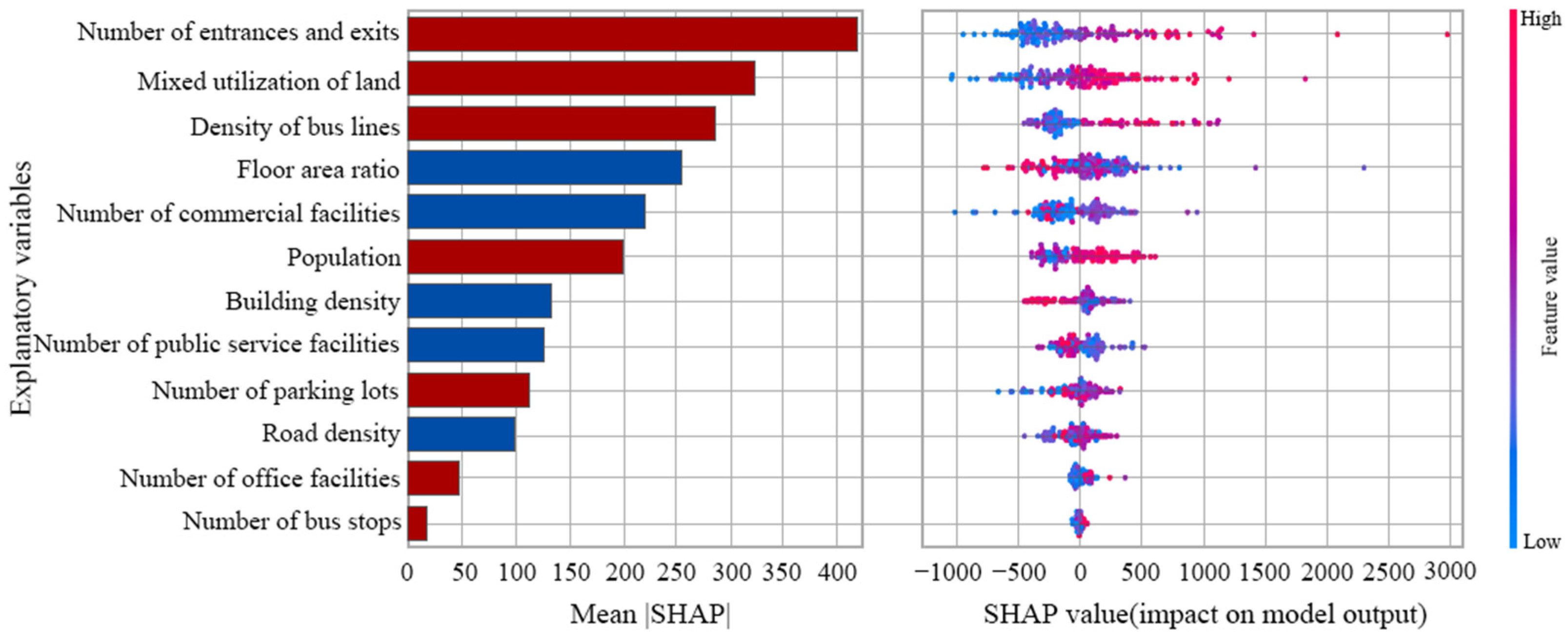
5.2. Global Impact on Metro Ridership

The average value of the absolute value of each explanatory variable SHAP is calculated and the influence degree of the explanatory variable on metro ridership is expressed. The greater the mean value of SHAP, the greater the influence of the explanatory variables on metro ridership and vice versa. The results of the average SHAP values of the explanatory variables for ridership at metro stations in different zones are shown in Figure 5 and Figure 6, with positive correlations in red and negative correlations in blue.

For metro stations inside the 4th Ring Road, the top three explanatory variables in the order of the influence degree are the number of entrances and exits > mixed utilization of land > the density of bus lines. There is a positive relationship between all three explanatory variables and SHAP values (Figure 5), i.e., the larger the eigenvalues of these three explanatory variables, the larger the SHAP values. This means that the larger these three explanatory variables are, the greater the impact on metro ridership. The mixed utilization of land has a large impact on metro ridership. That proves that the mixed utilization of land development has a strong promoting effect on metro ridership. That is consistent with the existing research [21]. However, as a very important index of land development, the floor area ratio is negatively correlated with metro ridership. It is proved that for the metro station in the 4th Ring Road, the ridership of metro stations with a higher floor area ratio is not necessarily higher. The likely reason is that the higher floor area ratios are generally concentrated in the core commercial office areas, where the morning peak is dominated by alighting ridership and does not generate much boarding ridership. Conversely, residential cores can generate high boarding ridership, but have a relatively low floor area ratio due to design constraints. The effect of population on ridership at metro stations inside the 4th Ring Road is positive, which is consistent with existing studies [4,36].

For metro stations outside the 4th Ring Road, the top three explanatory variables in the order of the influence degree are the number of public services facilities > building density > road density (Figure 6). Building density is negatively correlated with metro ridership and road density is negatively correlated with metro ridership. And, the average SHAP value for the number of office facilities is much greater than the average SHAP values for building density and road density. This proves that for metro stations outside the 4th Ring Road, the number of public service facilities is the explanatory variable with the greatest degree of influence. That said, for metro stations outside the 4th Ring Road, it may be more effective to adjust the ridership of metro stations by adjusting the number of public service facilities.

Figure 5 and Figure 6 show that there is a significant difference in the ranking of the effects of the explanatory variables on metro ridership inside and outside the 4th Ring Road. This demonstrates the need for this study partition to examine the built environment’s impact on metro ridership. Understanding the global impact of built environment explanatory variables on metro ridership in both zones can help planning decision makers and operations and design departments to adjust metro ridership from a zone-wide perspective.

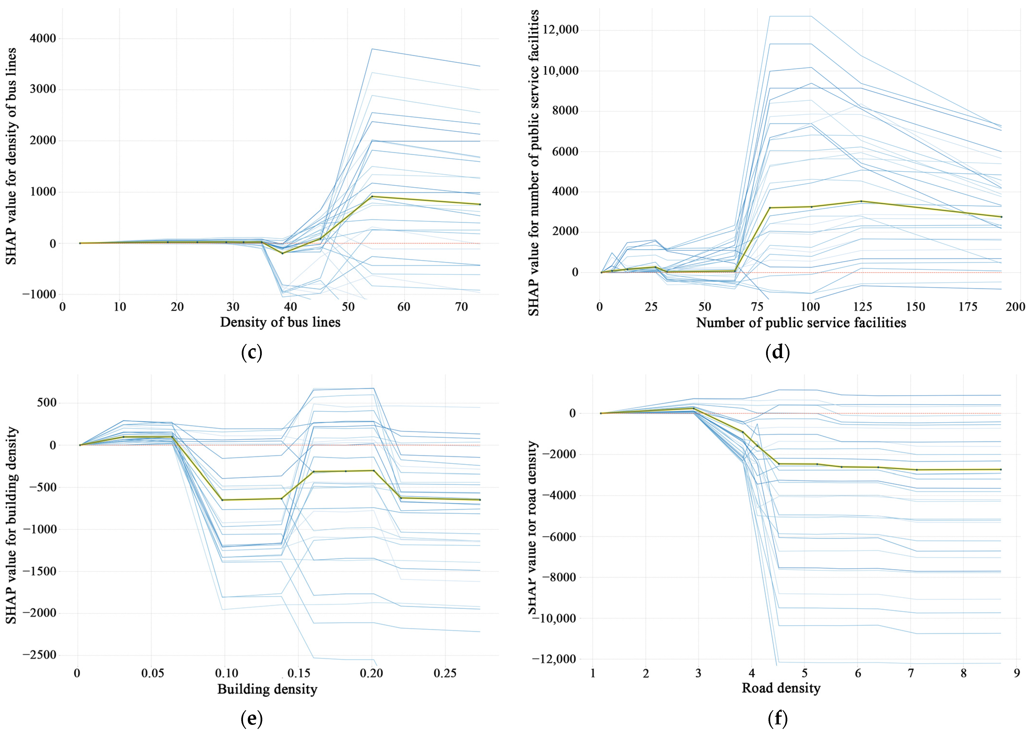
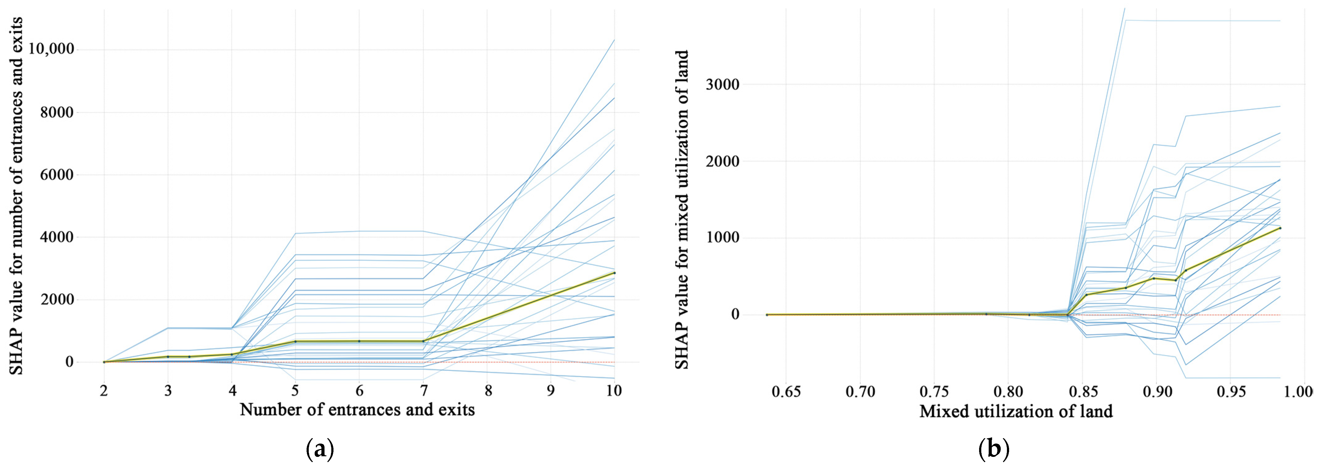
5.3. Nonlinear Effects on Metro Ridership

We select the top three explanatory variables for nonlinear analysis according to the influence degree of explanatory variables in the two zones. Figure 7 shows the nonlinear results for the explanatory variables for metro stations inside and outside the 4th Ring Road. For metro stations inside the 4th Ring Road, the relationship between the number of entrances and exits and metro ridership is overall positively correlated. When the number of entrances and exits is between five and seven, the effect of the number of entrances and exits on metro ridership is stable. This means that if we want to adjust the ridership at a metro station, adjusting the number of entrances in the range of 5–7 may not change the ridership at the metro station. However, when the number of entrances and exits is greater than seven, the impact of the number of entrances and exits on metro ridership tends to increase (Figure 7a). When the mixed utilization of land is less than 0.84, the impact of the mixed utilization of land on metro ridership is minimal (Figure 7b) and the overall impact of the mixed utilization of land on metro ridership is positive. If we want to improve the ridership of a metro station inside the 4th Ring Road, it may be more effective to increase the land use mix degree beyond 0.84. The nonlinear effect of the density of bus lines on metro ridership is more complex. When the density of the bus line is less than 35, the effect of the bus line density on metro ridership is less. At the same time, when the density of the bus line is in the range of 35–39, the effect of the bus line density on ridership is negative. In addition, when the density of bus lines is greater than 54, the effect of the bus line density on ridership is also negative (Figure 7c).

For metro stations outside the 4th Ring Road, when the number of public service facilities is less than 65, the impact of the number of public service facilities on the ridership at metro stations is small. However, when the number of public service facilities is in the range of 65–80, the impact of the number of public service facilities on the ridership at metro stations increases sharply. At the same time, when the number of public service facilities is greater than 80, the influence of the number of public service facilities on the ridership of the metro station tends to level off and there is even a negative correlation (Figure 7d). The overall impact of building density on metro ridership is negative. The effect of building density on metro ridership decreases sharply when building density is in the range of 0.07–0.10. The effect of building density on metro ridership is relatively flat when the building density is greater than 0.10 (Figure 7e). The effect of road density on metro ridership decreases sharply when the road density is between 1.9 and 4.5, but levels off when the road density is greater than 4.5 (Figure 7f). This demonstrates that the 1.9–4.5 range is the most effective if road density is to be used to change metro ridership.

We find the selected explanatory variables have a strong threshold effect on the ridership of the metro station. That is consistent with existing research findings [3,21]. Understanding the nonlinear effects of explanatory variables on metro ridership can help us to adjust metro ridership from an urban renewal perspective. In particular, we find that some of the explanatory variables do not have a greater impact on metro ridership at higher eigenvalues. Therefore, while understanding the global impact of the explanatory variables on metro ridership, the nonlinear impact of the explanatory variables on metro ridership needs to be considered simultaneously.

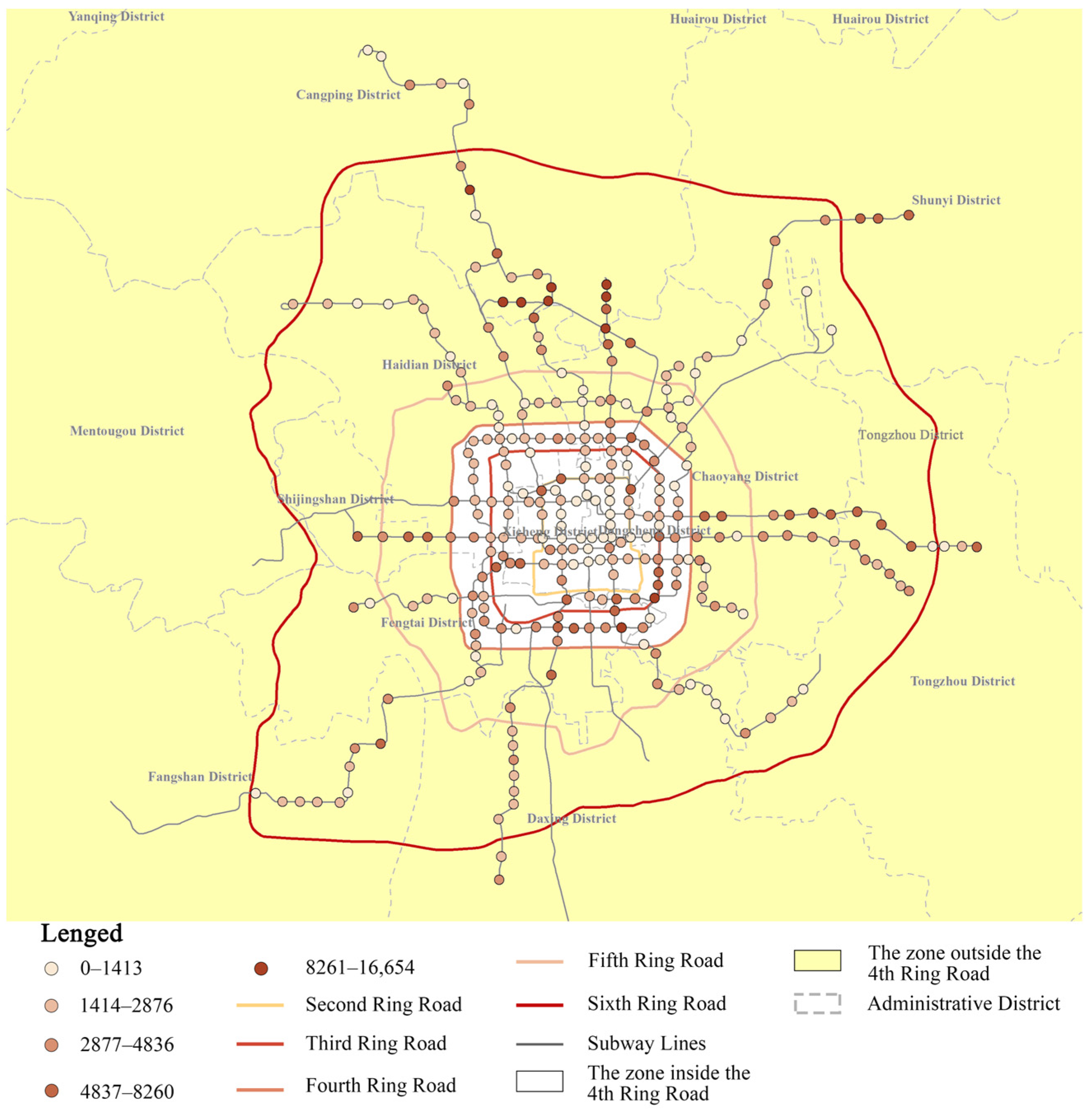
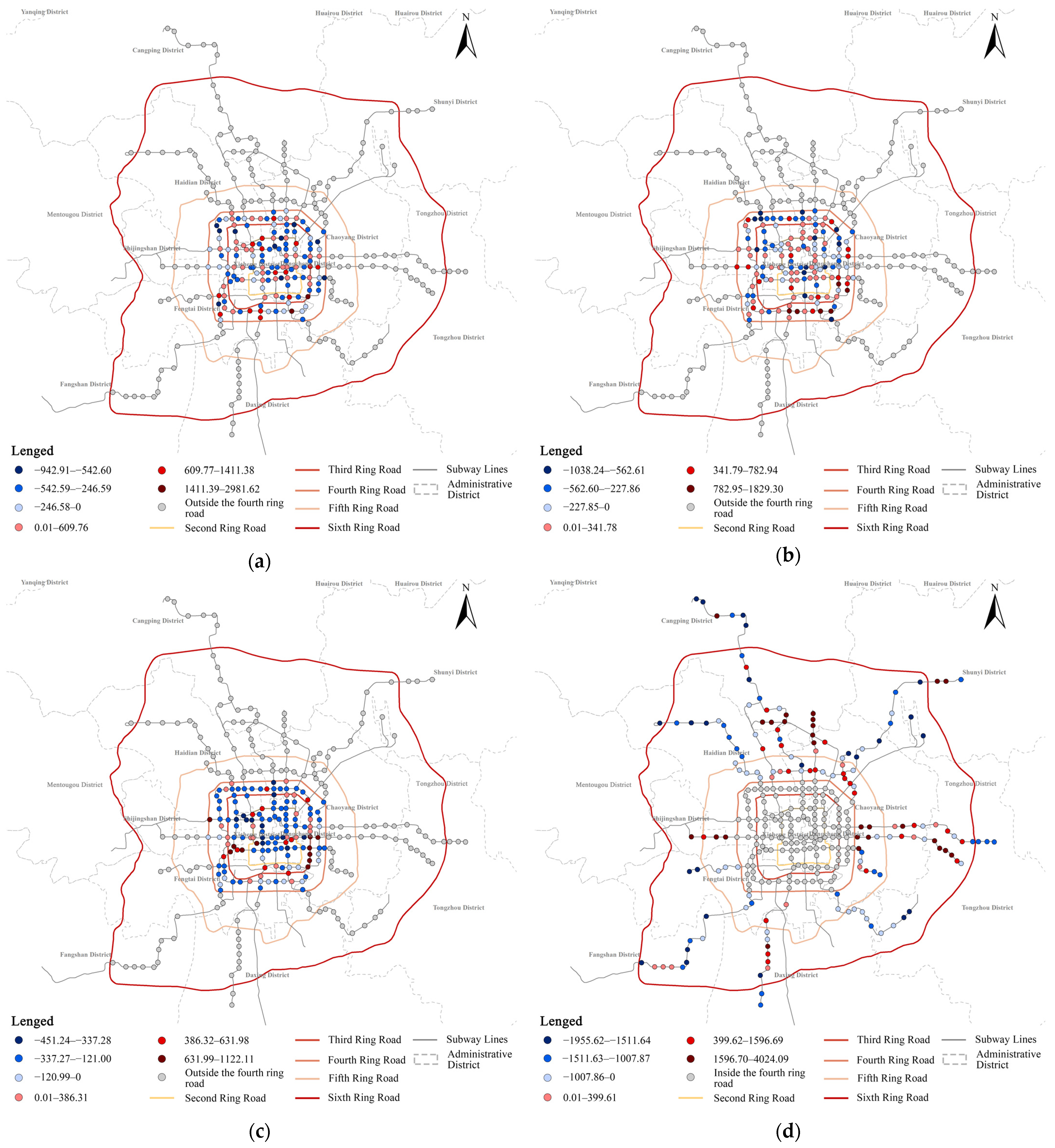
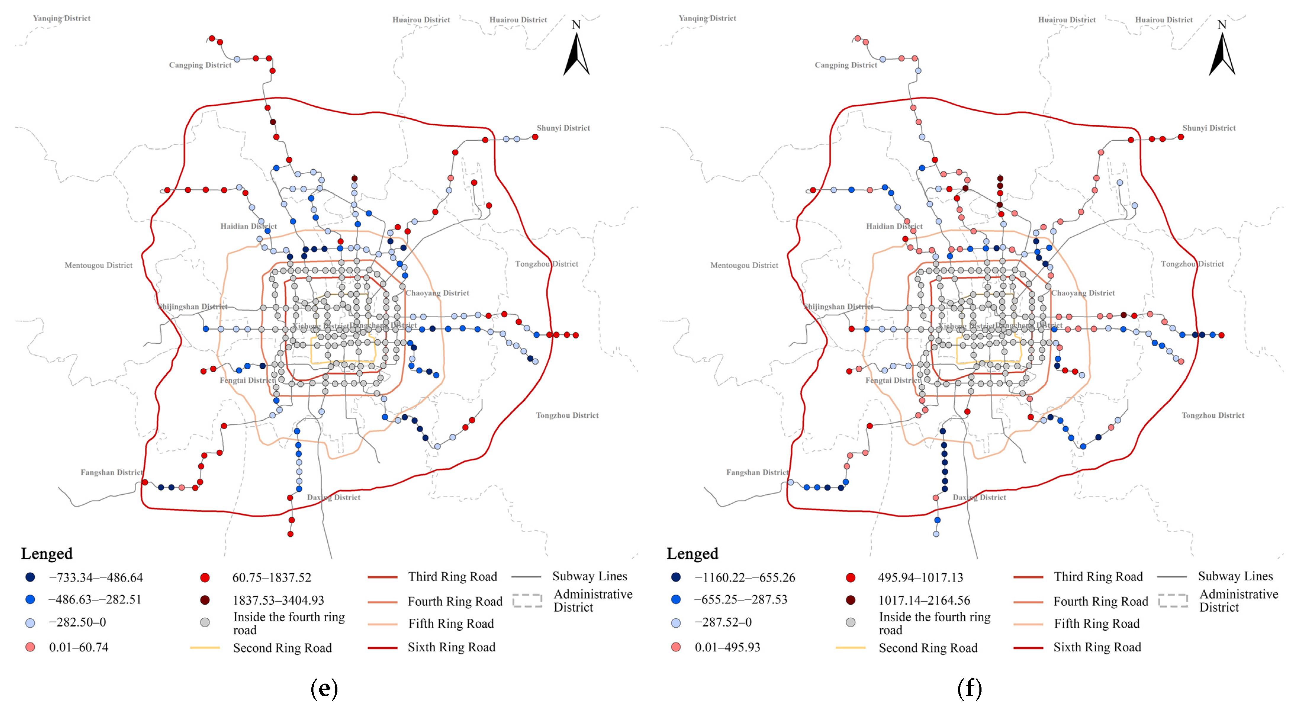
5.4. Spatial Heterogeneity Effecton Metro Ridership

Previous studies have mostly used Partial Dependence Plot (PDP) dependency maps to study the impact of the built environment explanatory variables on metro ridership from a global perspective [3,21]. However, existing research has demonstrated spatial heterogeneity in the influence of the built environment explanatory variables on metro ridership [17,18] and that the influence of built environment explanatory variables on metro ridership varies depending on the station’s location. Therefore, this study links SHAP values to metro stations and visualizes them. In this section, the top three global influences of the explanatory variables are still selected for spatial heterogeneity analysis. The results of the visualization of metro station SHAP values are shown in Figure 8.

For metro stations inside the 4th Ring Road, the number of metro stations with positive and negative SHAP values for the number of entrances and exits are roughly evenly divided. The metro stations with high negative SHAP values are mainly located in the northern part of the 4th Ring Road. The likely reason for this is that these metro stations are saturated with passengers, and further upgrading the number of entrances and exits to the metro stations will not enhance metro ridership. In addition, the metro stations with positive high SHAP values are mainly located in the southeastern part of the 4th Ring Road (Figure 8a). For the mixed utilization of land, there are more negative SHAP metro stations than positive SHAP metro stations (Figure 8b). This demonstrates that for most metro stations inside the 4th Ring Road, the mixed utilization of land dampens metro ridership. The reason for this may be that these neighborhoods are functionally mixed. However, it is a fact that where there is a high density of residential areas, there is also a high level of ridership at metro stations, and an excessive mix of land use reduces the number of residential areas. In addition, metro stations with negative SHAP values are clustered inside the 4th Ring Road. Therefore, when urban renewal is carried out later, the agglomeration area of metro stations with negative SHAP values can be considered uniformly. For the density of bus lines, the number of metro stations with negative SHAP values is much greater than the number of positive SHAP value metro stations (Figure 8c). This demonstrates that the density of bus lines has a dampening effect on metro ridership for most metro stations inside the 4th Ring Road. There is also a strong concentration of positive high SHAP metro stations, with positive high SHAP metro stations concentrated in the southeast and southwest inside the 4th Ring Road.

For the metro stations outside the 4th Ring Road, the number of public service facilities with positive high SHAP values metro stations are clustered in the north and east of outside the 4th Ring Road (Figure 8d). Combined with Figure 1, the ridership at the metro stations with positive high SHAP values is high, and we can reduce the ridership at the metro stations by reducing the number of public service facilities. Also, most of the stations with high negative SHAP are concentrated at the end of the metro line (Figure 7d). The possible reason is that these metro stations are located in suburban areas, where there may be some large infrastructure and public service facilities, and these facilities lead to fewer residential neighborhoods. The metro stations with positive building density SHAP are mainly concentrated at the end of the metro line (Figure 8e). And, the ridership of these metro stations are low, so we can enhance the ridership of these metro stations by increasing the building density. In addition, the stations with high negative SHAP have a strong agglomeration effect, especially in the north of the 4th to 5th Ring Road and the southeastern outside the 4th Ring Road (Figure 8e). And, these metro stations can be considered unified as a solution to regional problems. For road density, the stations with high negative SHAP are mostly concentrated at the end of Line 4 and in the northeast of the 4th to 5th Ring Road (Figure 8f). The probable reason is that these neighborhoods are in dense residential areas and are very densely populated. Increasing the road density will reduce the area of land to be used, which will result in smaller residential areas. And, the positive high SHAP stations are concentrated in the north outside the 4th Ring Road (Figure 7f).

By visualizing the values of the explanatory variables SHAP, we find the effect of the explanatory variables on the ridership of different metro stations. This has substantial practical implications for adjusting the ridership of individual metro stations [17,18]. When adjusting for individual metro ridership, we need to consider the SHAP values of the metro stations and the nonlinear effects of the explanatory variables on the ridership.

6. Conclusions

This research provides empirical evidence for the delineation of the PCA of metro stations in analyzing the nonlinear impacts of the built environment on the ridership of metro stations by using the XGBoost model. The optimal PCAs of metro stations inside the 4th Ring Road and outside the 4th Ring Road are the circular buffer zones with a radius of 800 m and 1300 m, respectively. Additionally, for the key explanatory variables (top three in overall impact) in the two zones we selected, there is a nonlinear relationship and a strong threshold effect on metro ridership. We also found spatial heterogeneity in the effects of the explanatory variables on ridership at metro stations. It indicates that we can develop site-specific renewal strategies around metro stations, considering the nonlinear effects of explanatory variables on metro ridership.

Based on the results of this study, we make the following recommendations: (1) we recommend that when considering the TOD range of Beijing, 800 m is recommended inside the 4th Ring Road and 1300 m is recommended outside the 4th Ring Road. (2) For the metro stations inside the 4th Ring Road, we can improve the vitality of the surrounding area by changing the land use mix degree and bus line density around the subway stations. For the metro station outside the 4th Ring Road, we can improve the vitality of the railway station by changing the number of public service facilities, building density, and road density.

There are some limitations in this study. First, assuming that the PCA is a circular buffer that cannot represent the actual range of passenger OD flow, this study did not use other means to judge the actual travel distribution of metro passenger flow, which may be important to improve the model accuracy. Second, OSM data was used in our study and this non-specialized map data can bias the results. In addition, socioeconomic variables were not included in our study, which can be included in future studies to make the model results more accurate.

References

1. Sung, H.; Choi, K.; Lee, S.; Cheon, S. Exploring the impacts of land use by service coverage and station-level accessibility on rail transit ridership. J. Transp. Geogr. 2014, 36, 134–140. [Google Scholar] [CrossRef]
2. Chiou, Y.-C.; Jou, R.-C.; Yang, C.-H. Factors affecting public transportation usage rate: Geographically weighted regression. Transp. Res. Part A Policy Pract. 2015, 78, 161–177. [Google Scholar] [CrossRef]
3. Gan, Z.; Yang, M.; Feng, T.; Timmermans, H.J.P. Examining the relationship between built environment and metro ridership at station-to-station level. Transp. Res. Part D Transp. Environ. 2020, 82, 102332. [Google Scholar] [CrossRef]
4. Zhao, J.; Deng, W.; Song, Y.; Zhu, Y. What influences Metro station ridership in China? Insights from Nanjing. Cities 2013, 35, 114–124. [Google Scholar] [CrossRef]
5. Li, S.; Liu, X.; Li, Z.; Wu, Z.; Yan, Z.; Chen, Y.; Gao, F. Spatial and Temporal Dynamics of Urban Expansion along the Guangzhou–Foshan Inter-City Rail Transit Corridor, China. Sustainability 2018, 10, 593. [Google Scholar] [CrossRef]
6. Shen, Q.; Chen, P.; Pan, H. Factors affecting car ownership and mode choice in rail transit-supported suburbs of a large Chinese city. Transp. Res. Part A Policy Pract. 2016, 94, 31–44. [Google Scholar] [CrossRef]
7. Cullinane, S. The relationship between car ownership and public transport provision: A case study of Hong Kong. Transp. Policy 2002, 9, 29–39. [Google Scholar] [CrossRef]
8. Goodwin, P.B. Car ownership and public transport use: Revisiting the interaction. Transportation 1993, 20, 21–33. [Google Scholar] [CrossRef]
9. Nguyen-Phuoc, D.Q.; Currie, G.; De Gruyter, C.; Young, W. Congestion relief and public transport: An enhanced method using disaggregate mode shift evidence. Case Stud. Transp. Policy 2018, 6, 518–528. [Google Scholar] [CrossRef]
10. Badland, H.M.; Rachele, J.N.; Roberts, R.; Giles-Corti, B. Creating and applying public transport indicators to test pathways of behaviours and health through an urban transport framework. J. Transp. Health 2017, 4, 208–215. [Google Scholar] [CrossRef]
11. Currie, G. Quantifying spatial gaps in public transport supply based on social needs. J. Transp. Geogr. 2010, 18, 31–41. [Google Scholar] [CrossRef]
12. Cervero, R.; Day, J. Suburbanization and transit-oriented development in China. Transp. Policy 2008, 15, 315–323. [Google Scholar] [CrossRef]
13. Huang, X.; Cao, X.; Cao, X.; Yin, J. How does the propensity of living near rail transit moderate the influence of rail transit on transit trip frequency in Xi’an? J. Transp. Geogr. 2016, 54, 194–204. [Google Scholar] [CrossRef]
14. Central People’s Government of the People’s Republic of China. Modern Comprehensive Transport System Development Plan for the Fourteenth Five-Year Plan. Available online: http://www.gov.cn/zhengce/content/2022-01/18/content_5669049.htm (accessed on 12 April 2023).
15. Gazette, P. Beijing Underground’s Daily Passenger Volume Breaks 11 Million, Some Stations Will Start to Take Temporary Flow Restriction Measures in the Morning Rush Hour. Available online: https://baijiahao.baidu.com/s?id=1758039502843960181&wfr=spider&for=pc (accessed on 23 May 2023).
16. Zhao, J.; Deng, W.; Song, Y.; Zhu, Y. Analysis of Metro ridership at station level and station-to-station level in Nanjing: An approach based on direct demand models. Transportation 2013, 41, 133–155. [Google Scholar] [CrossRef]
17. Wang, Z.; Song, J.; Zhang, Y.; Li, S.; Jia, J.; Song, C. Spatial Heterogeneity Analysis for Influencing Factors of Outbound Ridership of Subway Stations Considering the Optimal Scale Range of “7D” Built Environments. Sustainability 2022, 14, 16314. [Google Scholar] [CrossRef]
18. Du, Q.; Zhou, Y.; Huang, Y.; Wang, Y.; Bai, L. Spatiotemporal exploration of the non-linear impacts of accessibility on metro ridership. J. Transp. Geogr. 2022, 102, 103380. [Google Scholar] [CrossRef]
19. Ji, S.; Wang, X.; Lyu, T.; Liu, X.; Wang, Y.; Heinen, E.; Sun, Z. Understanding cycling distance according to the prediction of the XGBoost and the interpretation of SHAP: A non-linear and interaction effect analysis. J. Transp. Geogr. 2022, 103, 103414. [Google Scholar] [CrossRef]
20. Caigang, Z.; Shaoying, L.; Zhangzhi, T.; Feng, G.; Zhifeng, W. Nonlinear and threshold effects of traffic condition and built environment on dockless bike sharing at street level. J. Transp. Geogr. 2022, 102, 103375. [Google Scholar] [CrossRef]
21. Ding, C.; Cao, X.; Liu, C. How does the station-area built environment influence Metrorail ridership? Using gradient boosting decision trees to identify non-linear thresholds. J. Transp. Geogr. 2019, 77, 70–78. [Google Scholar] [CrossRef]
22. Jun, M.-J.; Choi, K.; Jeong, J.-E.; Kwon, K.-H.; Kim, H.-J. Land use characteristics of subway catchment areas and their influence on subway ridership in Seoul. J. Transp. Geogr. 2015, 48, 30–40. [Google Scholar] [CrossRef]
23. Li, S.; Lyu, D.; Huang, G.; Zhang, X.; Gao, F.; Chen, Y.; Liu, X. Spatially varying impacts of built environment factors on rail transit ridership at station level: A case study in Guangzhou, China. J. Transp. Geogr. 2020, 82, 102631. [Google Scholar] [CrossRef]
24. Li, S.; Lyu, D.; Liu, X.; Tan, Z.; Gao, F.; Huang, G.; Wu, Z. The varying patterns of rail transit ridership and their relationships with fine-scale built environment factors: Big data analytics from Guangzhou. Cities 2020, 99, 102580. [Google Scholar] [CrossRef]
25. Shao, Q.; Zhang, W.; Cao, X.; Yang, J.; Yin, J. Threshold and moderating effects of land use on metro ridership in Shenzhen: Implications for TOD planning. J. Transp. Geogr. 2020, 89, 102878. [Google Scholar] [CrossRef]
26. Robert, C.; Kara, K. Travel Demand and the 3Ds: Density, Diversity, and Design. Transp. Res. Part D Transp. Environ. 1997, 2, 199–219. [Google Scholar]
27. Frank, L.D.; Gary, P. Impacts of Mixed Use and Density on Utilization of Three Modes of Travel: Single-Occupant Vehicle, Transit, and Walking. Transp. Res. Rec. 1994, 1994, 44–52. [Google Scholar]
28. Todd, M.; Reid, E. Transit-Oriented Development in the Sun Belt. Transp. Res. Rec. 1996, 1552, 145–153. [Google Scholar]
29. Chanam, L.; Moudon, A.V. Correlates of Walking for Transportation or Recreation Purposes. J. Phys. Act. Health 2006, 3, S77–S98. [Google Scholar]
30. Kuby, M.; Barranda, A.; Upchurch, C. Factors influencing light-rail station boardings in the United States. Transp. Res. Part A Policy Pract. 2004, 38, 223–247. [Google Scholar] [CrossRef]
31. Sohn, K.; Shim, H. Factors generating boardings at Metro stations in the Seoul metropolitan area. Cities 2010, 27, 358–368. [Google Scholar] [CrossRef]
32. Zhao, J.; Deng, W. Relationship of Walk Access Distance to Rapid Rail Transit Stations with Personal Characteristics and Station Context. J. Urban Plan. Dev. 2013, 139, 311–321. [Google Scholar] [CrossRef]
33. Gutiérrez, J.; Cardozo, O.D.; García-Palomares, J.C. Transit ridership forecasting at station level: An approach based on distance-decay weighted regression. J. Transp. Geogr. 2011, 19, 1081–1092. [Google Scholar] [CrossRef]
34. Sung, H.; Oh, J.-T. Transit-oriented development in a high-density city: Identifying its association with transit ridership in Seoul, Korea. Cities 2011, 28, 70–82. [Google Scholar] [CrossRef]
35. Loo, B.P.Y.; Chen, C.; Chan, E.T.H. Rail-based transit-oriented development: Lessons from New York City and Hong Kong. Landsc. Urban Plan. 2010, 97, 202–212. [Google Scholar] [CrossRef]
36. Cardozo, O.D.; García-Palomares, J.C.; Gutiérrez, J. Application of geographically weighted regression to the direct forecasting of transit ridership at station-level. Appl. Geogr. 2012, 34, 548–558. [Google Scholar] [CrossRef]
37. Calvo, F.; Eboli, L.; Forciniti, C.; Mazzulla, G. Factors influencing trip generation on metro system in Madrid (Spain). Transp. Res. Part D Transp. Environ. 2019, 67, 156–172. [Google Scholar] [CrossRef]
38. Lu, B.; Yang, W.; Ge, Y.; Harris, P. Improvements to the calibration of a geographically weighted regression with parameter-specific distance metrics and bandwidths. Comput. Environ. Urban Syst. 2018, 71, 41–57. [Google Scholar] [CrossRef]
39. Andersson, D.E.; Shyr, O.F.; Yang, J. Neighbourhood effects on station-level transit use: Evidence from the Taipei metro. J. Transp. Geogr. 2021, 94, 103127. [Google Scholar] [CrossRef]
40. Yu, L.; Cong, Y.; Chen, K. Determination of the Peak Hour Ridership of Metro Stations in Xi’an, China Using Geographically-Weighted Regression. Sustainability 2020, 12, 2255. [Google Scholar] [CrossRef]
41. Cheng, L.; Chen, X.; De Vos, J.; Lai, X.; Witlox, F. Applying a random forest method approach to model travel mode choice behavior. Travel Behav. Soc. 2019, 14, 1–10. [Google Scholar] [CrossRef]
42. Hagenauer, J.; Helbich, M. A comparative study of machine learning classifiers for modeling travel mode choice. Expert Syst. Appl. 2017, 78, 273–282. [Google Scholar] [CrossRef]
43. Zhao, X.; Yan, X.; Yu, A.; Van Hentenryck, P. Prediction and behavioral analysis of travel mode choice: A comparison of machine learning and logit models. Travel Behav. Soc. 2020, 20, 22–35. [Google Scholar] [CrossRef]
44. Liu, M.; Liu, Y.; Ye, Y. Nonlinear effects of built environment features on metro ridership: An integrated exploration with machine learning considering spatial heterogeneity. Sustain. Cities Soc. 2023, 95, 104613. [Google Scholar] [CrossRef]
45. Liang, W.; Luo, S.; Zhao, G.; Wu, H. Predicting Hard Rock Pillar Stability Using GBDT, XGBoost, and LightGBM Algorithms. Mathematics 2020, 8, 765. [Google Scholar] [CrossRef]
46. Chen, T.; Guestrin, C. XGBoost: A Scalable Tree Boosting System. In Proceedings of the 22nd ACM SIGKDD International Conference on Knowledge Discovery and Data Mining, San Francisco, CA, USA, 13–17 August 2016; pp. 785–794. [Google Scholar]
47. Kim, S.; Lee, S. Nonlinear relationships and interaction effects of an urban environment on crime incidence: Application of urban big data and an interpretable machine learning method. Sustain. Cities Soc. 2023, 91, 104419. [Google Scholar] [CrossRef]
48. Sun, B.; Sun, T.; Jiao, P.; Tang, J. Spatio-Temporal Segmented Traffic Flow Prediction with ANPRS Data Based on Improved XGBoost. J. Adv. Transp. 2021, 2021, 5559562. [Google Scholar] [CrossRef]
49. Ran, D.; Jiaxin, H.; Yuzhe, H. Application of a Combined Model based on K-means++ and XGBoost in Traffic Congestion Prediction. In Proceedings of the 2020 5th International Conference on Smart Grid and Electrical Automation (ICSGEA), Zhangjiajie, China, 13–14 June 2020; pp. 413–418. [Google Scholar]
50. Lv, C.X.; An, S.Y.; Qiao, B.J.; Wu, W. Time series analysis of hemorrhagic fever with renal syndrome in mainland China by using an XGBoost forecasting model. BMC Infect. Dis. 2021, 21, 839. [Google Scholar] [CrossRef]
51. Tang, J.; Zheng, L.; Han, C.; Liu, F.; Cai, J. Traffic Incident Clearance Time Prediction and Influencing Factor Analysis Using Extreme Gradient Boosting Model. J. Adv. Transp. 2020, 2020, 6401082. [Google Scholar] [CrossRef]
52. Liu, J.; Wang, B.; Xiao, L. Non-linear associations between built environment and active travel for working and shopping: An extreme gradient boosting approach. J. Transp. Geogr. 2021, 92, 103034. [Google Scholar] [CrossRef]
53. Yang, L.; Ao, Y.; Ke, J.; Lu, Y.; Liang, Y. To walk or not to walk? Examining non-linear effects of streetscape greenery on walking propensity of older adults. J. Transp. Geogr. 2021, 94, 103099. [Google Scholar] [CrossRef]
54. Yang, C.; Chen, M.; Yuan, Q. The application of XGBoost and SHAP to examining the factors in freight truck-related crashes: An exploratory analysis. Accid. Anal. Prev. 2021, 158, 106153. [Google Scholar] [CrossRef]
55. Zhou, S.; Liu, Z.; Wang, M.; Gan, W.; Zhao, Z.; Wu, Z. Impacts of building configurations on urban stormwater management at a block scale using XGBoost. Sustain. Cities Soc. 2022, 87, 104235. [Google Scholar] [CrossRef]
56. Estupiñán, N.; Rodríguez, D.A. The relationship between urban form and station boardings for Bogotá’s BRT. Transp. Res. Part A Policy Pract. 2008, 42, 296–306. [Google Scholar] [CrossRef]
57. Sun, L.S.; Wang, S.W.; Yao, L.Y.; Rong, J.; Ma, J.M. Estimation of transit ridership based on spatial analysis and precise land use data. Transp. Lett. 2016, 8, 140–147. [Google Scholar] [CrossRef]
58. Thompson, G.; Brown, J.; Bhattacharya, T. What Really Matters for Increasing Transit Ridership: Understanding the Determinants of Transit Ridership Demand in Broward County, Florida. Urban Stud. 2012, 49, 3327–3345. [Google Scholar] [CrossRef]
59. Ewing, R.; Cervero, R. Travel and the Built Environment. J. Am. Plan. Assoc. 2010, 76, 265–294. [Google Scholar] [CrossRef]
60. De Gruyter, C.; Saghapour, T.; Ma, L.; Dodson, J. How does the built environment affect transit use by train, tram and bus? J. Transp. Land Use 2020, 13, 625–650. [Google Scholar] [CrossRef]
61. An, D.; Tong, X.; Liu, K.; Chan, E.H.W. Understanding the impact of built environment on metro ridership using open source in Shanghai. Cities 2019, 93, 177–187. [Google Scholar] [CrossRef]
62. Chen, E.; Ye, Z.; Wang, C.; Zhang, W. Discovering the spatio-temporal impacts of built environment on metro ridership using smart card data. Cities 2019, 95, 102359. [Google Scholar] [CrossRef]
63. Jiang, Y.; Christopher Zegras, P.; Mehndiratta, S. Walk the line: Station context, corridor type and bus rapid transit walk access in Jinan, China. J. Transp. Geogr. 2012, 20, 1–14. [Google Scholar] [CrossRef]
64. Gao, W.; Wang, W.; Dimitrov, D.; Wang, Y. Nano properties analysis via fourth multiplicative ABC indicator calculating. Arab. J. Chem. 2018, 11, 793–801. [Google Scholar] [CrossRef]
65. Lundberg, S.M.; Su-In, L. A Unified Approach to Interpreting Model Predictions. In Proceedings of the 31st Annual Conference on Neural Information Processing Systems (NIPS 2017), Long Beach, CA, USA, 4–9 December 2017; pp. 4765–4774. [Google Scholar]
66. de Myttenaere, A.; Golden, B.; Le Grand, B.; Rossi, F. Mean Absolute Percentage Error for regression models. Neurocomputing 2016, 192, 38–48. [Google Scholar] [CrossRef]
Figure 1. Spatial distribution of metro ridership during the morning peak hours.
Applsci 13 12210 g001
Figure 2. Changes in metro ridership by the time of day in Beijing.
Applsci 13 12210 g002
Figure 3. Accuracy of different machine learning models: (a) Inside the 4th Ring Road; (b) Outside the 4th Ring Road.
Applsci 13 12210 g003
Figure 4. MAPE diagram for different zones of metro station PCAs.
Applsci 13 12210 g004
Figure 5. Global impact of explanatory variables on metro ridership inside the 4th Ring Road.
Applsci 13 12210 g005
Figure 6. Global impact of explanatory variables on metro ridership outside the 4th Ring Road.
Applsci 13 12210 g006
Figure 7. Nonlinear results for explanatory variables of metro stations inside and outside the 4th Ring Road: (a) Number of entrances and exits for metro stations inside the 4th Ring Road. (b) Mixed utilization of land for metro stations inside the 4th Ring Road. (c) Density of bus lines for metro stations inside the 4th Ring Road. (d) Number of public service facilities for metro stations outside the 4th Ring Road. (e) Building density for metro stations outside the 4th Ring Road. (f) Road density for metro stations outside the 4th Ring Road.
Applsci 13 12210 g007aApplsci 13 12210 g007b
Figure 8. Local SHAP values for metro stations inside and outside the 4th Ring Road: (a) Number of entrances and exits for metro stations inside the 4th Ring Road. (b) Mixed utilization of land for metro stations inside the 4th Ring Road. (c) Density of bus lines for metro stations inside the 4th Ring Road. (d) Number of public service facilities for metro stations outside the 4th Ring Road. (e) Building density for metro stations outside the 4th Ring Road. (f) Road density for metro stations outside the 4th Ring Road.
Applsci 13 12210 g008aApplsci 13 12210 g008b