Review

Machine Learning Methods in Weather and Climate Applications: A Survey

1
School of Computer Science and Engineering, University of New South Wales, Sydney, NSW 2052, Australia
2
Commonwealth Scientific and Industrial Research Organisation, Data 61, Sydney, NSW 2015, Australia
3
Key Laboratory of Meteorological Disaster, Nanjing University of Information Science and Technology, Nanjing 210044, China
*
Author to whom correspondence should be addressed.
Appl. Sci. 2023, 13(21), 12019; https://doi.org/10.3390/app132112019
Submission received: 9 September 2023 / Revised: 22 October 2023 / Accepted: 28 October 2023 / Published: 3 November 2023
(This article belongs to the Special Issue Methods and Applications of Data Management and Analytics)

Abstract

:
With the rapid development of artificial intelligence, machine learning is gradually becoming popular for predictions in all walks of life. In meteorology, it is gradually competing with traditional climate predictions dominated by physical models. This survey aims to consolidate the current understanding of Machine Learning (ML) applications in weather and climate prediction—a field of growing importance across multiple sectors, including agriculture and disaster management. Building upon an exhaustive review of more than 20 methods highlighted in existing literature, this survey pinpointed eight techniques that show particular promise for improving the accuracy of both short-term weather and medium-to-long-term climate forecasts. According to the survey, while ML demonstrates significant capabilities in short-term weather prediction, its application in medium-to-long-term climate forecasting remains limited, constrained by factors such as intricate climate variables and data limitations. Current literature tends to focus narrowly on either short-term weather or medium-to-long-term climate forecasting, often neglecting the relationship between the two, as well as general neglect of modeling structure and recent advances. By providing an integrated analysis of models spanning different time scales, this survey aims to bridge these gaps, thereby serving as a meaningful guide for future interdisciplinary research in this rapidly evolving field.

1. Introduction

Weather and climate prediction play an important role in human history. Weather forecasting serves as a critical tool that underpins various facets of human life and social operations, permeating everything from individual decision-making to large-scale industrial planning. Its significance at the individual level is manifested in its capacity to guide personal safety measures, from avoiding hazardous outdoor activities during inclement weather to taking health precautions in extreme temperatures. This decision-making extends into the agricultural realm, where forecasts inform the timing for planting, harvesting, and irrigation, ultimately contributing to maximized crop yields and stable food supply chains [1]. The ripple effect of accurate forecasting also reaches the energy sector, where it aids in efficiently managing demand fluctuations, allowing for optimized power generation and distribution. This efficiency is echoed in the transportation industry, where the planning and scheduling of flights, train routes, and maritime activities hinge on weather conditions. Precise weather predictions are key to mitigating delays and enhancing safety protocols [2]. Beyond these sectors, weather forecasting plays an integral role in the realm of construction and infrastructure development. Adverse conditions can cause project delays and degrade quality, making accurate forecasts a cornerstone of effective project management. Moreover, the capacity to forecast extreme weather events like hurricanes and typhoons is instrumental in disaster management, offering the possibility of early warnings and thereby mitigating loss of life and property [3].
Although climate prediction is often ignored by human beings in the short term, it has a close relationship with Earth’s life. Global warming and the subsequent rise in sea levels constitute critical challenges with far-reaching implications for the future of our planet. Through sophisticated climate modeling and forecasting techniques, we stand to gain valuable insights into the potential ramifications of these phenomena, thereby enabling the development of targeted mitigation strategies. For instance, precise estimations of sea-level changes in future decades could inform rational urban planning and disaster prevention measures in coastal cities. On an extended temporal scale, climate change is poised to instigate considerable shifts in the geographical distribution of numerous species, thereby jeopardizing biodiversity. State-of-the-art climate models integrate an array of variables—encompassing atmospheric conditions, oceanic currents, terrestrial ecosystems, and biospheric interactions—to furnish a nuanced comprehension of environmental transformations [4]. This integrative approach is indispensable for the formulation of effective global and regional policies aimed at preserving ecological diversity. Economic sectors such as agriculture, fisheries, and tourism are highly susceptible to the vagaries of climate change. Elevated temperatures may precipitate a decline in crop yields, while an upsurge in extreme weather events stands to impact tourism adversely. Longitudinal climate forecasts are instrumental in guiding governmental and business strategies to adapt to these inevitable changes. Furthermore, sustainable resource management, encompassing water, land, and forests, benefits significantly from long-term climate projections. Accurate predictive models can forecast potential water scarcity in specific regions, thereby allowing for the preemptive implementation of judicious water management policies. Climate change is also implicated in a gamut of public health crises, ranging from the proliferation of infectious diseases to an uptick in heatwave incidents. Comprehensive long-term climate models can equip public health agencies with the data necessary to allocate resources and devise effective response strategies.
Table 1 elucidates the diverse applications of weather forecasting across multiple sectors and time frames. In the short-term context, weather forecasts are instrumental for agricultural activities such as determining the optimal timing for sowing and harvesting crops, as well as formulating irrigation and fertilization plans. In the energy sector, short-term forecasts facilitate accurate predictions of output levels for wind and solar energy production. For transportation, which encompasses road, rail, aviation, and maritime industries, real-time weather information is vital for operational decisions affecting safety and efficiency. Similarly, construction projects rely on short-term forecasts for planning and ensuring safe operations. In the retail and sales domains, weather forecasts enable businesses to make timely inventory adjustments. For tourism and entertainment, particularly those involving outdoor activities and attractions, short-term forecasts provide essential guidance for day-to-day operations. Furthermore, short-term weather forecasts play a pivotal role in environmental and disaster management by providing early warnings for floods, fires, and other natural calamities. In the medium-to-long-term scenario, weather forecasts have broader implications for strategic planning and risk assessment. In agriculture, these forecasts are used for long-term land management and planning. The insurance industry utilizes medium-to-long-term forecasts to prepare for prospective increases in specific types of natural disasters, such as floods and droughts. Real estate sectors also employ these forecasts for evaluating the long-term impact of climate-related factors like sea level rise. Urban planning initiatives benefit from these forecasts for effective water resource management. For the tourism industry, medium-to-long-term weather forecasts are integral for long-term investments and for identifying regions that may become popular tourist destinations in the future. Additionally, in the realm of public health, long-term climate changes projected through these forecasts can inform strategies for controlling the spread of diseases. In summary, weather forecasts serve as a vital tool for both immediate and long-term decision-making across a diverse range of sectors.
Short-term weather prediction. Short-term weather forecasting primarily targets weather conditions that span from a few hours up to seven days, aiming to deliver highly accurate and actionable information that empowers individuals to make timely decisions like carrying an umbrella or postponing outdoor activities. These forecasts typically decrease in reliability as they stretch further into the future. Essential elements of these forecasts include maximum and minimum temperatures, the likelihood and intensity of various forms of precipitation like rain, snow, or hail, wind speed and direction, levels of relative humidity or dew point temperature, and types of cloud cover such as sunny, cloudy, or overcast conditions [18]. Visibility distance in foggy or smoky conditions and warnings about extreme weather events like hurricanes or heavy rainfall are also often included. The methodologies for generating these forecasts comprise numerical simulations run on high-performance computers, the integration of observational data from multiple sources like satellites and ground-based stations, and statistical techniques that involve pattern recognition and probability calculations based on historical weather data. While generally more accurate than long-term forecasts, short-term predictions are not without their limitations, often influenced by the quality of the input data, the resolution of the numerical models, and the sensitivity to initial atmospheric conditions. These forecasts play a crucial role in various sectors, including decision-making processes, transportation safety, and agriculture, despite the inherent complexities and uncertainties tied to predicting atmospheric behavior.
Medium-to-long-term climate prediction. Medium-to-long-term climate forecasting (MLTF) concentrates on projecting climate conditions over periods extending from several months to multiple years, in contrast to short-term weather forecasts, which focus more on immediate atmospheric conditions. The time frame of these climate forecasts can be segmented into medium-term, which generally ranges from a single season up to a year, and long-term, which could span years to decades or even beyond [19]. Unlike weather forecasts, which may provide information on imminent rainfall or snowfall, MLTF centers on the average states or trends of climate variables, such as average temperature and precipitation, ocean-atmosphere interactions like El Niño or La Niña conditions, and the likelihood of extreme weather events like droughts or floods, as well as anticipated hurricane activities [20]. The projection also encompasses broader climate trends, such as global warming or localized climatic shifts. These forecasts employ a variety of methods, including statistical models based on historical data and seasonal patterns, dynamical models that operate on complex mathematical equations rooted in physics, and integrated models that amalgamate multiple data sources and methodologies. However, the accuracy of medium- to long-term climate forecasting often falls short when compared with short-term weather predictions due to the intricate, multi-scale, and multi-process interactions that constitute the climate system, not to mention the lack of exhaustive long-term data. The forecasts’ reliability can also be influenced by socio-economic variables, human activities, and shifts in policy. Despite these complexities, medium-to-long-term climate projections serve pivotal roles in areas such as resource management, agricultural planning, disaster mitigation, and energy policy formulation, making them not only a multi-faceted, multi-disciplinary challenge but also a crucial frontier in both climate science and applied research.
Survey Scope. In recent years, machine learning has emerged as a potent tool in meteorology, displaying strong capabilities in feature abstraction and trend prediction. Numerous studies have employed machine learning as the principal methodology for weather forecasting [21,22]. Our survey extends this current understanding by including recent advances in the application of machine learning techniques such as High-Resolution Neural Networks and 3D neural networks, representing the state-of-the-art in this multidisciplinary domain. This survey endeavors to serve as a comprehensive review of machine learning techniques applied in the realms of meteorology and climate prediction. Previous studies have substantiated the efficacy of machine learning methods in short-term weather forecasting [23]. However, there exists a conspicuous dearth of nuanced research in the context of medium-to-long-term climate predictions [24]. The primary objective of this survey is to offer a comprehensive analysis of nearly 20 diverse machine-learning methods applied in meteorology and climate science. It is worth noting that our selection criteria are twofold: we include classic models in the application of machine learning to meteorology, as well as, from a computer science perspective, represent recent state-of-the-art complex models. We categorize these methods based on their temporal applicability: short-term weather forecasting and medium-to-long-term climate predictions. This dual focus uniquely situates our survey as a bridge between immediate weather forecasts and longer climatic trends, thereby filling existing research gaps summarized as follows:
  • Limited Scope: Existing surveys predominantly focus either on short-term weather forecasting or medium-to-long-term climate predictions. There is a notable absence of comprehensive surveys that endeavour to bridge these two-time scales. In addition, current investigations tend to focus narrowly on specific methods, such as simple neural networks, thereby neglecting some combination of methods.
  • Lack of model details: Many extisting studies offer only generalized viewpoints and lack a systematic analysis of the specific model employed in weather and climate prediction. This absence creates a barrier for researchers aiming to understand the intricacies and efficacy of individual methods.
  • Neglect of Recent Advances: Despite rapid developments in machine learning and computational techniques, existing surveys have not kept pace with these advancements. The paucity of information on cutting-edge technologies stymies the progression of research in this interdisciplinary field.
By addressing these key motivations, this survey aims to serve as a roadmap for future research endeavors in this rapidly evolving, interdisciplinary field.
Contributions of the Survey. The contributions of this paper are as follows.
  • Comprehensive scope: Unlike research endeavors that restrict their inquiry to a singular temporal scale, our survey provides a comprehensive analysis that amalgamates short-term weather forecasting with medium- and long-term climate predictions. In total, 20 models were surveyed, of which a select subset of eight were chosen for in-depth scrutiny. These models are discerned as the industry’s avant-garde, thereby serving as invaluable references for researchers. For instance, the PanGu model exhibits remarkable congruence with actual observational results, thereby illustrating the caliber of the models included in our analysis.
  • In-Depth Analysis: Breaking new ground, this study delves into the intricate operational mechanisms of the eight focal models. We have dissected the operating mechanisms of these eight models, distinguishing the differences in their approaches and summarizing the commonalities in their methods through comparison. This comparison helps readers gain a deeper understanding of the efficacy and applicability of each model and provides a reference for choosing the most appropriate model for a given scenario.
  • Identification of Contemporary Challenges and Future Work: The survey identifies pressing challenges currently facing the field, such as the limited dataset of chronological seasons and complex climate change effects, and suggests directions for future work, including simulating datasets and physics-based constraint models. These recommendations not only add a forward-looking dimension to our research but also act as a catalyst for further research and development in climate prediction.
Outline of the paper. This paper consists of six sections. Section 1 describes our motivation and innovations compared with other weather prediction surveys. Section 2 introduces some weather-related background knowledge. Section 3 broadly introduces relevant methods for weather prediction other than machine learning. Section 4 highlights the milestones of forecasting models using machine learning and their categorization. Section 5 and Section 6 analyze representative methods on both short-term and medium- and long-term time scales. Section 7 and Section 8 summarize the challenges faced, present promising future work, and conclude the paper.

2. Background

In this section, the objective is to provide a thorough understanding of key meteorological principles, tailored to be accessible even to readers outside the meteorological domain. The section commences with an overview of Reanalysis Data, the cornerstone for data inputs in weather forecasting and climate projection models. Following this, the focus shifts to the vital aspect of model output validation. It is necessary to identify appropriate benchmarks and key performance indicators for assessing the model’s predictive accuracy. Without well-defined standards, the evaluation of a model’s effectiveness remains nebulous. Furthermore, three essential concepts—bias-correction, down-scaling, and emulation—are introduced. These become particularly relevant when discussing the role of machine learning in augmenting physical models. Finally, the text offers an in-depth explanation of predicting extreme events, clearly defining “extreme event” and differentiating them from routine occurrences.
Data source. Observed data undergoes a series of rigorous processing steps before it enters the predictive model (or what is known as the reanalysis data generation process). They are amassed from heterogeneous sources, such as ground-based networks like the Global Historical Climatology Network (GHCN), atmospheric tools like Next-Generation Radar (NEXRAD), and satellite systems like the Geostationary Operational Environmental Satellites (GOES). Oceanic measurements are captured through the specialized ARGO float network, focusing on key parameters like temperature and salinity. These raw datasets are further audited for quality control, spatial and temporal interpolation, and unit standardization.
Despite meticulous preprocessing, observational data exhibit challenges such as spatial-temporal heterogeneity, inherent measurement errors, and discrepancies with numerical models. To mitigate these issues, data assimilation techniques are employed. These techniques synergize observations with model forecasts using mathematical and statistical algorithms like Kalman filtering, Three-Dimensional Variational Analysis (3D-Var), and Four-Dimensional Variational Analysis (4D-Var) [25].
Additionally, data assimilation can be utilized to enhance the initial model conditions and correct systemic model biases. The scope of data assimilation extends beyond singular meteorological models to complex Earth System Models that integrate dynamics from atmospheric, oceanic, and terrestrial subsystems. Post-assimilation, where the model state is updated, leads to the generation of “reanalysis data”. Popular reanalysis datasets include ERA5 from the European Centre for Medium-Range Weather Forecasts (ECMWF), NCEP/NCAR Reanalysis from the National Centers for Environmental Prediction and the National Center for Atmospheric Research, JRA-55 from the Japan Meteorological Agency, and MERRA-2 from NASA.
Result evaluation. Result evaluation serves as a critical stage in the iterative process of predictive modeling. It involves comparing forecasted outcomes against observed data to gauge the model’s reliability and accuracy. The temporal dimension is a critical factor in result evaluation. Short-term predictive models, like those used in weather forecasting, benefit from near-real-time feedback, which allows for frequent recalibration using machine learning algorithms like Ensemble Kalman Filters. On the other hand, long-term models, such as climate projections based on General Circulation Models (GCMs), are constrained by the absence of an immediate validation period. In weather forecasting, meteorologists employ a variety of numerical models, like the Weather Research and Forecasting (WRF) model, which are evaluated based on short-term observational data. Standard metrics for evaluation include Mean Absolute Error (MAE), Root Mean Square Error (RMSE), and Skill Scores. The high-frequency availability of data from sources like weather radars and satellites facilitates rapid iterations and refinements. In contrast, climate models are scrutinized using different methodologies. Given their long-term nature, climate models are often validated using historical and paleoclimatic data. Statistical techniques like Empirical Orthogonal Functions (EOF) and Principal Component Analysis (PCA) are employed to identify and validate overarching climatic patterns. These models often have to account for high levels of uncertainty and are cross-validated against geological or even astronomical records, making immediate validation impractical. For weather forecasts, predictive accuracy within the scope of hours to days is paramount. Climate models, conversely, are evaluated based on their ability to accurately reproduce decadal and centennial patterns.
Bias correction. In the context of meteorology, climate science, machine learning, and statistical modeling, bias correction (or bias adjustment) refers to a set of techniques used to correct systematic errors (biases) in model simulations or predictions. These biases may arise due to various factors such as model limitations, uncertainties in parameterization, or discrepancies between model assumptions and real-world data. Bias Correction (Bias Adjustment) can be formally defined as the process of modifying the output of predictive models to align more closely with observed data. The primary objective is to minimize the difference between the model’s estimates and the observed values, thereby improving the model’s accuracy and reliability.
In more formal terms, let M represent the model output and O represent the observed data. Bias B is defined as:
B = M O
The aim of bias-correction is to find a function f such that:
f ( M ) O
Various methods can be employed for bias-correction, including simple linear adjustments, quantile mapping, and more complex machine-learning techniques. The choice of method often depends on the specific characteristics of the data and the overarching objectives of the study.
Emulation. The term emulation is utilized here to denote the approach where machine learning models are employed to simulate or approximate components and processes of the original physical model. In meteorology, physical models are devised based on a comprehensive understanding of atmospheric dynamics, often entailing intricate hydrodynamic equations to elucidate atmospheric motions and interactions. However, to attain high computational efficiency in practical operations, direct resolution of these equations is frequently computationally demanding, particularly when high spatial and temporal resolution simulations are requisite. To alleviate these issues, modelers are already using fast and accurate ML simulations to simulate existing time-consuming parameterizations [26,27,28]. Machine learning methods are capable of delivering fast and precise approximations of complex physical processes by learning patterns and relationships from historical data or high-precision model runs. For instance, neural networks or other machine learning algorithms can be deployed to deal with Longwave and shortwave radiation parameterization [29,30] and emulate nonlinear wave interactions in wind wave models [31]. Consequently, machine learning models can substitute traditional physical parameterization schemes in prediction models, significantly alleviating the computational burden while preserving or even augmenting the accuracy of predictions.
Down-scaling. Down-scaling in meteorology and climate science is a computational technique employed to bridge the gap between the spatial and temporal resolutions offered by General Circulation Models (GCMs) or Regional Climate Models (RCMs) and the scale at which specific applications, such as local weather predictions or hydrological assessments, operate. Given that GCMs and RCMs typically operate at a coarse resolution—spanning tens or hundreds of kilometers—Down-scaling aims to refine these projections to a more localized level, potentially down to single kilometers or less.
Extreme events. In meteorology, an “extreme event” refers to a rare occurrence within a statistical distribution of a particular weather variable. These events can be extreme high temperatures, heavy precipitation, severe storms, or high winds, among others. These phenomena are considered “extreme” due to their rarity and typically severe impact on ecosystems, infrastructure, and human life.
Symbol definition. Since many formulas are involved in weather and climate prediction methods, we have defined an Abbreviation in the end of paper that summarizes all the common symbols and their definitions.
In standard meteorological models, precipitation is usually represented as a three-dimensional array containing latitude, longitude, and elevation. Each cell in this array contains a numerical value that represents the expected precipitation for that particular location and elevation during a given time window. This data structure allows for straightforward visualization and analysis, such as contour maps or time series plots. Unlike standard precipitation forecasts, which focus primarily on the water content of the atmosphere, extreme events may require tracking multiple variables simultaneously. For example, hurricane modeling may include variables such as wind speed, atmospheric pressure, and sea surface temperature. Given the higher uncertainty associated with extreme events, the output may not be a single deterministic forecast but rather a probabilistic one. An integration approach can be used to generate multiple model runs to capture a range of possible outcomes. Both types of predictions are typically evaluated using statistical metrics; however, for extreme events, more sophisticated measures such as event detection rates, false alarm rates, or skill scores associated with probabilistic predictions can be used.

3. Related Work

This study principally centers on the utilization of machine learning techniques in the realm of climate prediction. However, to furnish a comprehensive perspective, we also elucidate traditional forecasting methodologies—statistical and physical methods—within this section. Historically speaking, the evolution of predictive models in climate science has undergone three distinct phases. Initially, statistical methods were prevalently deployed; however, their limited accuracy led to their gradual supplantation by physical models. While the role of statistical methods has dwindled in terms of standalone application, they are frequently amalgamated with other techniques to enhance predictive fidelity. Subsequently, physical models ascended to become the prevailing paradigm in climate prediction. Given the current predominance of physical models in the field of climate prediction, they serve as the natural benchmarks against which we evaluate the performance of emerging machine learning approaches. Finally, our focus is on machine learning methods, exploring their potential to mitigate the limitations intrinsic to their historical predecessors.

3.1. Statistical Method

Statistical or empirical forecasting methods have a rich history in meteorology, serving as the initial approach to weather prediction before the advent of computational models. Statistical prediction methodologies serve as the linchpin for data-driven approaches in meteorological forecasting, focusing on both short-term weather patterns and long-term climatic changes. These methods typically harness powerful statistical algorithms, among which Geographically Weighted Regression (GWR) and Spatio-Temporal Kriging (ST-Kriging) stand out as particularly effective [32,33].
GWR is instrumental in adjusting for spatial heterogeneity, allowing meteorological variables to exhibit different relationships depending on their geographical context. ST-Kriging extends this spatial consideration to include the temporal domain, thereby capturing variations in weather and climate that are both location-specific and time-sensitive. Such spatio-temporal modeling is especially pertinent in a rapidly changing environment, where traditional stationary models often fail to capture the dynamism inherent in meteorological systems.
Forecasting using inter-annual increments is now a statistically based forecasting method with better results. The interannual increment of a variable such as precipitation is calculated as:
Interannual Increment = Value year Value year 1
Through meticulous analysis of variables correlating with the inter-annual growth rate of the predictive variable, five key predictive factors have been identified. A multivariate linear regression model was developed, employing these selected key predictive factors to estimate the inter-annual increment for future time units. The estimated inter-annual increment is subsequently aggregated with the actual variable value from the preceding year to generate a precise prediction of the total quantity for the current time frame.
However, these statistical models operate on a critical assumption cited in literature [34,35], which posits that the governing laws influencing past meteorological events are consistent and thus applicable to future events as well. While this assumption generally holds for many meteorological phenomena, it confronts limitations when dealing with intrinsically chaotic systems. The Butterfly Effect serves as a prime example of such chaotic behavior, where minuscule perturbations in initial conditions can yield dramatically divergent outcomes. This implies that the reliability of statistical models could be compromised when predicting phenomena susceptible to such chaotic influences.

3.2. Physical Models

Physical models were the predominant method for meteorological forecasting before the advent of Artificial Intelligence (AI) and generally produce more accurate results compared with statistical methods. Physical models are predicated upon a foundational set of physical principles, including but not limited to Newton’s laws of motion, the laws of conservation of energy and mass, and the principles of thermodynamics. These governing equations are commonly expressed in mathematical form, with the Navier–Stokes equations serving as a quintessential example for describing fluid dynamics. At the core of these models lies the objective of simulating real-world phenomena in a computational setting with high fidelity. To solve these intricate equations, high-performance computing platforms are typically employed, complemented by specialized numerical methods and techniques such as Computational Fluid Dynamics (CFD) and Finite Element Analysis (FEA).
In the context of atmospheric science, these physical models are especially pivotal for Numerical Weather Prediction (NWP) and climate modeling. NWP primarily focuses on short-to-medium-term weather forecasting, striving for highly accurate meteorological predictions within a span of days or weeks. In contrast, climate models concentrate on long-term changes and predictions, which can span months, years, or even longer time scales. Owing to their rigorous construction based on physical laws, physical models offer a high degree of accuracy and reliability, providing researchers with valuable insights into the underlying mechanisms of weather and climate variations.
As mentioned before, statistical-based methods can analyze past weather data to make predictions, but they may often fail to accurately predict future weather trends [36], and physic-based models, despite being computationally intensive [37], help us understand atmospheric, oceanic, and terrestrial processes in detail. Recently, machine learning methods have begun to be applied to the field of meteorology [38], offering new ways to analyze and predict weather patterns and climate change [39]. Machine learning methods are increasingly being utilized in meteorology for forecasting. Compared to physical models, they offer faster predictions, and compared with statistical methods, they provide more accurate results [40]. Additionally, machine learning can be employed for error correction and Down-scaling, further enhancing its applicability in weather and climate predictions.
In the critical fields of weather forecasting and climate prediction, achieving accuracy and efficiency is of paramount importance. Traditional methods, while foundational, inevitably present limitations, creating a compelling need for innovative approaches. Machine learning has emerged as a promising solution, demonstrating significant potential for enhancing prediction outcomes.

4. Taxonomy of Climate Prediction Applications

In this section, we primarily explore the historical trajectory of machine learning applications within the field of meteorology. We categorize the surveyed methods according to distinct criteria, facilitating a more lucid understanding for the reader.

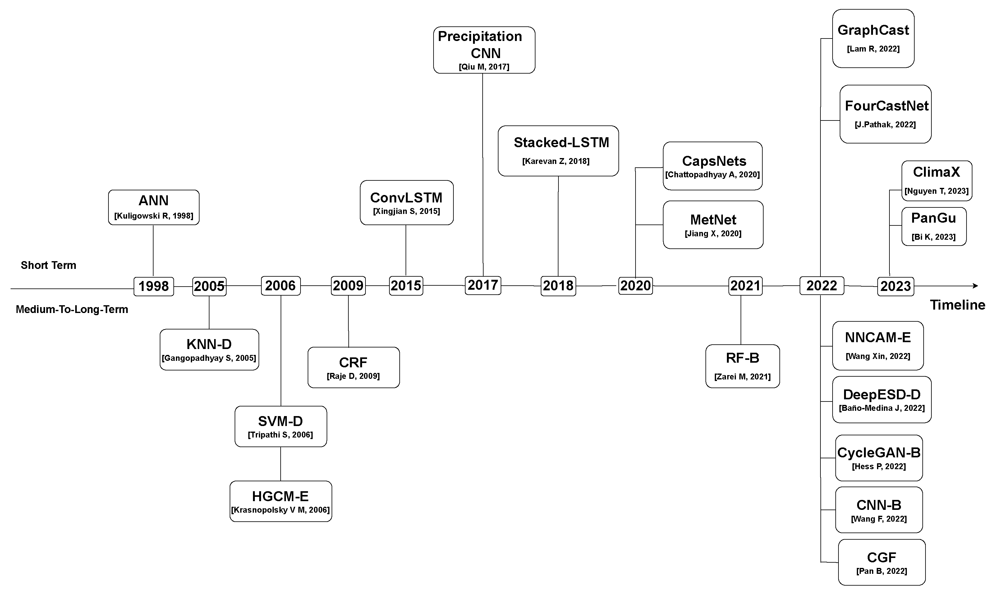
4.1. Climate Prediction Milestone Based on Machine-Learning

In this subsection, we surveyed almost 20 methods of machine learning applications for weather prediction and climate prediction. These methods are representative and common. We listed them in the following timeline shown in Figure 1. The journey of machine learning applications in climate and weather prediction has undergone significant transformations since their inception.
Climate prediction methods before 2010. The earliest model in this context is the Precipitation Neural Network Prediction Model, published in 1998. This model serves as an archetype of Basic DNN Models, leveraging Artificial Neural Networks to offer short-term forecasts specifically for precipitation in the Middle Atlantic Region. Advancing to the mid-2000s, the realm of medium-to-long-term predictions saw the introduction of ML-Enhanced Non-Deep-Learning Models, exemplified by KNN-Down-scaling in 2005 and SVM-Down-scaling in 2006. These models employed machine learning techniques like K-Nearest Neighbors and Support Vector Machines, targeting localized precipitation forecasts in the United States and India, respectively. In 2009, the field welcomed another medium-to-long-term model, CRF-Down-scaling, which used Conditional Random Fields to predict precipitation in the Mahanadi Basin.
Climate prediction methods from 2010–2019. During the period from 2010 to 2019, the field of weather prediction witnessed significant technological advancements and diversification in modeling approaches. Around 2015, a notable shift back to short-term predictions was observed with the introduction of Hybrid DNN Models, exemplified by ConsvLSTM. This model integrated Long Short-Term Memory networks with Convolutional Neural Networks to provide precipitation forecasts specifically for Hong Kong. As the decade progressed, models became increasingly specialized. For instance, the 2017 Precipitation Convolution prediction model leveraged Convolutional Neural Networks to focus on localized precipitation forecasts in Guang Dong, China. The following year saw the emergence of the Stacked-LSTM-Model, which utilized Long Short-Term Memory networks for temperature predictions in Amsterdam and Eindhoven.
Climate prediction methods from 2020. Fast forward to 2020, the CapsNet model, a Specific Model, leveraged a novel architecture known as Capsule Networks to predict extreme weather events in North America. By 2021, the scope extended to models like RF-bias-correction and the sea-ice prediction model, focusing on medium-to-long-term predictions. The former employed Random Forests for precipitation forecasts in Iran, while the latter utilized probabilistic deep learning techniques for forecasts in the Arctic region. Recent advancements as of 2022 and 2023 incorporate more complex architectures. Cycle GAN, a 2022 model, utilized Generative Adversarial Networks for global precipitation prediction. PanGu, a 2023 release, employed 3D Neural Networks for predicting extreme weather events globally. Another recent model, FourCastNet, leverages a technique known as AFNO to predict extreme global events. Furthermore, in 2022, this year also witnessed the introduction of DeepESD-Down-scaling and CNN-Bias-correction models, both utilizing Convolutional Neural Networks to predict local temperature scales and perform global bias correction, respectively.

4.2. Classification of Climate Prediction Methods

To provide a deeper level of understanding regarding the various weather prediction methods discussed, we have organized them into classifications in Table 2. These classifications are made according to multiple criteria that encompass Time Scale, Type, Model, Technique, Name, Region, and Event. This structured approach aims to offer readers an easy way to compare and contrast different methods, as well as to gain insights into the specific contexts where each method is most applicable.
Time Scale. Models in weather and climate prediction are initially divided based on their temporal range into ’Short-term’ and ’Medium-to-long-term’. Short-term weather prediction focuses on the state of the atmosphere in the short term, usually the weather conditions in the next few hours to days. Medium-to-long-term climate prediction focuses on longer time scales, usually the average weather trends over months, years, or decades. Weather forecasts focus on specific weather conditions in the near term, such as temperature, precipitation, humidity, wind speed, and direction. Climate prediction focuses on long-term weather patterns and trends, such as seasonal or inter-annual variations in temperature and precipitation. In the traditional approach, weather forecasting usually utilizes numerical weather prediction models that predict weather changes in the short term by resolving the equations of atmospheric dynamics; climate prediction usually utilizes climate models that incorporate more complex interacting feedback mechanisms and longer-term external drivers, such as greenhouse gas emissions and changes in solar radiation.
Spatial Scale. Regional meteorology concerns a specified geographic area, such as a country or a continent, and aims to provide detailed insights into the weather and climate phenomena within that domain. The finer spatial resolution of regional models allows for a more nuanced understanding of local geographical and topographical influences on weather patterns, which in turn can lead to more accurate forecasts within that particular area. On the other hand, global meteorology encompasses the entire planet’s atmospheric conditions, providing a broader yet less detailed view of weather and climate phenomena. The spatial resolution of global models is generally coarser compared with regional models. As such, global forecasts might not capture localized weather events as accurately as regional forecasts. However, global models are crucial for understanding large-scale atmospheric dynamics and providing the boundary conditions necessary for regional models.
ML and ML-Enhanced Types. We categorize models into ML and ML-Enhanced types. In ML type, algorithms are directly applied to climate data for pattern recognition or predictive tasks. These algorithms typically operate independently of traditional physical models, relying instead on data-driven insights garnered from extensive climate datasets. Contrastingly, ML-Enhanced models integrate machine learning techniques into conventional physical models to optimize or enhance their performance. Fundamentally, these approaches still rely on physical models for prediction. However, machine learning algorithms serve as auxiliary tools for parameter tuning, feature engineering, or addressing specific limitations in the physical models, thereby improving their overall predictive accuracy and reliability. In this survey, ML-enhanced was divided into three catagories: bias correction, down-scaling, and emulation [66]. Model. Within each time scale, models are further categorized by their type. These models include: Specific Models: These are unique or specialized neural network architectures developed for particular applications.
Specific DNN Models: Unique or specialized neural network architectures developed for particular applications.
Hybrid DNN Models: These models use a combination of different neural network architectures, such as LSTM + CNN.
Single DNN Models: These models employ foundational Deep Neural Network architectures like ANNs (Artificial Neural Networks), CNNs (Convolutional Neural Networks), and LSTMs (Long Short-Term Memory networks).
Non-Deep-Learning Models: These models incorporate machine learning techniques that do not rely on deep learning, such as Random Forests and Support Vector Machines.
Technique. This category specifies the underlying machine learning or deep learning technique used in a particular model, for example, CNN, LSTM, Random Forest, Probalistic Deep Learning, and GAN.
CNN. A specific type of ANN is the Convolutional Neural Network (CNN), designed to automatically and adaptively learn spatial hierarchies from data [67]. CNNs comprise three main types of layers: convolutional, pooling, and fully connected [68]. The convolutional layer applies various filters to the input data to create feature maps, identifying spatial hierarchies and patterns. Pooling layers reduce dimensionality, summarizing features in the previous layer [69]. Fully connected layers then perform classification based on the high-level features identified [70]. CNNs are particularly relevant in meteorology for tasks like satellite image analysis, with their ability to recognize and extract spatial patterns [71]. Their unique structure allows them to capture local dependencies in the data, making them robust against shifts and distortions [72].
LSTM. Long Short-Term Memory (LSTM) units are a specialized form of recurrent neural network architecture [42]. Purposefully designed to mitigate the vanishing gradient problem inherent in traditional RNNs, LSTM units manage the information flow through a series of gates, namely the input, forget, and output gates. These gates govern the retention, forgetting, and output of information, allowing LSTMs to effectively capture long-range dependencies and temporal dynamics in sequential data [42]. In the context of meteorological forecasting, the utilization of LSTM contributes to a nuanced understanding of weather patterns as it retains relevant historical information and discards irrelevant details over various time scales [42]. The pioneering design of LSTMs and their ability to deal with nonlinear time dependencies have led to their outstanding robustness, adaptability, and efficiency, making them an essential part of modern predictive models [42].
Random forest. A technique used to adjust or correct biases in predictive models, particularly in weather forecasting or climate modeling. Random Forest (RF) is a machine learning algorithm used for various types of classification and regression tasks. In the context of bias correction, the Random Forest algorithm would be trained to identify and correct systematic errors or biases in the predictions made by a primary forecasting model.
Probabilistic deep learning. Probabilistic deep learning models in weather forecasting aim to provide not just point estimates of meteorological variables but also a measure of uncertainty associated with the predictions. By leveraging complex neural networks, these models capture intricate relationships between various features like temperature, humidity, and wind speed. The probabilistic aspect helps in quantifying the confidence in predictions, which is crucial for risk assessment and decision-making in weather-sensitive industries.
Generative adversarial networks. Generative Adversarial Networks (GANs) are a class of deep learning models composed of two neural networks: a Generator and a Discriminator. The Generator aims to produce data that closely resembles a genuine data distribution, while the discriminator’s role is to distinguish between real and generated data. During training, these networks engage in a kind of “cat-and-mouse” game, continually adapting and improving—ultimately with the goal of creating generated data so convincing that the Discriminator can no longer tell it apart from real data.
Graph Neural Network. Graph Neural Network (GNN) are designed to work with graph-structured data, capturing the relationships between connected nodes effectively. They operate by passing messages or aggregating information from neighbors and then updating each node’s representation accordingly. This makes GNNs exceptionally good at handling problems like social network analysis, molecular structure analysis, and recommendation systems.
Transformer. A transformer consists of an encoder and a decoder, but its most unique feature is the attention mechanism. This allows the model to weigh the importance of different parts of the input data, making it very efficient for tasks like text summarization, question answering, and language generation.
Name. Some models are commonly cited or recognized under a specific name, such as PanGu or FourCastNet. Some models are named after their technical features.
Event. The type of weather or climatic events that the model aims to forecast is specified under this category. This could range from generalized weather conditions like temperature and precipitation to more extreme weather events.
Selection Rationale. In the next section, we will discuss the related reasons. In the short term, we choose three specific ones (PanGu; GraphCast and FourCastNet) as analysis targets according to the model type. And we also analyze the MetNet, which is a hybrid DNNs Model. The other hybrid DNNs Model (ConsLSTM) is one part of MetNet. In the medium-to-long term, we choose the probabilistic deep learning model (Conditional Generative Forecasting). It has more extensive applicability compared with the other one in the probabilistic deep learning category. The probabilistic deep learning method is also a minority machine learning method that could be used in medium-to-long-term prediction. In addition, we also selected three machine learning-enhanced methods for Down-scaling: bias correction and emulation. In general, our survey includes established models recognized for their utility in applying machine learning to meteorological tasks and cutting-edge complex models viewed from a computer science standpoint as state-of-the-art.

5. Short-Term Weather Forecast
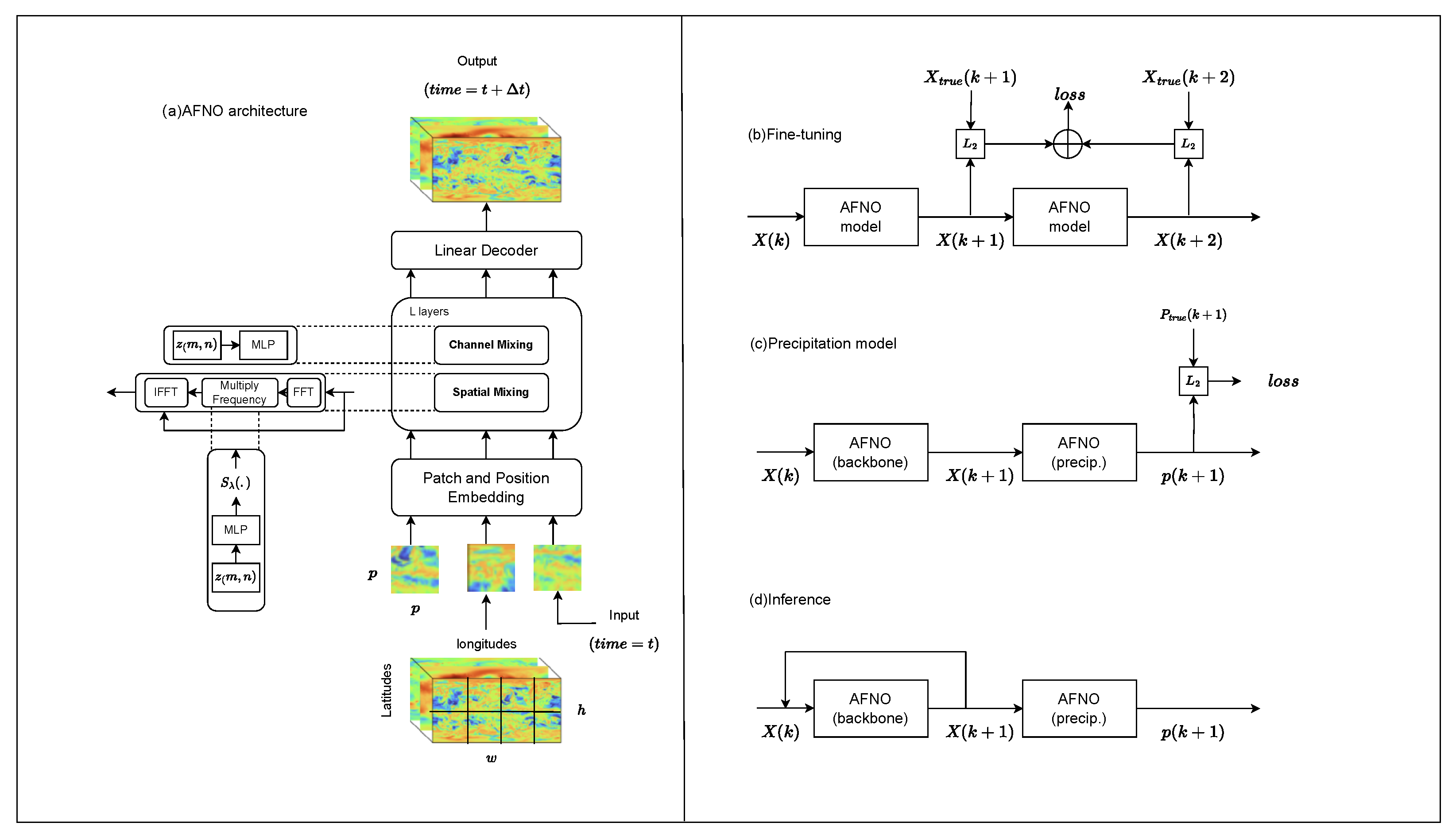
Weather forecasting aims to predict atmospheric phenomena within a short time-frame, generally ranging from one to three days. This information is crucial for a multitude of sectors, including agriculture, transportation, and emergency management. Factors such as precipitation, temperature, and extreme weather events are of particular interest. Forecasting methods have evolved over the years, transitioning from traditional numerical methods to more advanced hybrid and machine-learning models. This section elucidates the working principles, methodologies, and merits and demerits of traditional numerical weather prediction models, MetNet, FourCastNet, and PanGu.

5.1. Model Design

Numerical Weather Model Numerical Weather Prediction (NWP) stands as a cornerstone methodology in the realm of meteorological forecasting, fundamentally rooted in the simulation of atmospheric dynamics through intricate physical models. At the core of NWP lies a set of governing physical equations that encapsulate the holistic behavior of the atmosphere:
  • The Navier-Stokes Equations [73]: Serving as the quintessential descriptors of fluid motion, these equations delineate the fundamental mechanics underlying atmospheric flow.
    · v = 0
    ρ v t + v · v = p + μ 2 v + ρ g
  • The Thermodynamic Equations [74]: These equations intricately interrelate the temperature, pressure, and humidity within the atmospheric matrix, offering insights into the state and transitions of atmospheric energy.
    ρ t + · ( ρ v ) = 0 ( Continuity equation )
    T t + v · T = q c p ( Energy equation )
    D p D t = ρ c p · v ( Pressure equation )
The model is fundamentally based on a set of time-dependent partial differential equations, which require sophisticated numerical techniques for solving. The resolution of these equations enables the simulation of the inherently dynamic atmosphere, serving as the cornerstone for accurate and predictive meteorological insights. Within this overarching framework, a suite of integral components is embedded to address specific physical interactions that occur at different resolutions, such as cloud formation, radiation, convection, boundary layers, and surface interactions. Each of these components serves a pivotal role:
  • The Cloud Microphysics Parameterization Scheme is instrumental for simulating the life cycles of cloud droplets and ice crystals, thereby affecting [75,76] and atmospheric energy balance.
  • Shortwave and Longwave Radiation Transfer Equations elucidate the absorption, scattering, and emission of both solar and terrestrial radiation, which in turn influence atmospheric temperature and dynamics.
  • Empirical or Semi-Empirical Convection Parameterization Schemes simulate vertical atmospheric motions initiated by local instabilities, facilitating the capture of weather phenomena like thunderstorms.
  • Boundary-Layer Dynamics concentrates on the exchanges of momentum, energy, and matter between the Earth’s surface and the atmosphere which are crucial for the accurate representation of surface conditions in the model.
  • Land Surface and Soil/Ocean Interaction Modules simulate the exchange of energy, moisture, and momentum between the surface and the atmosphere, while also accounting for terrestrial and aquatic influences on atmospheric conditions.
These components are tightly coupled with the core atmospheric dynamics equations, collectively constituting a comprehensive, multi-scale framework. This intricate integration allows for the simulation of the complex dynamical evolution inherent in the atmosphere, contributing to more reliable and precise weather forecasting.
In Numerical Weather Prediction (NWP), a critical tool for atmospheric dynamics forecasting, the process begins with data assimilation, where observational data is integrated into the model to reflect current conditions. This is followed by numerical integration, where governing equations are meticulously solved to simulate atmospheric changes over time. However, certain phenomena, like the microphysics of clouds, cannot be directly resolved and are accounted for through parameterization to approximate their aggregate effects. Finally, post-processing methods are used to reconcile potential discrepancies between model predictions and real-world observations, ensuring accurate and reliable forecasts. This comprehensive process captures the complexity of weather systems and serves as a robust method for weather prediction [77]. While the sophistication of NWP allows for detailed simulations of global atmospheric states, one cannot overlook the intensive computational requirements of such models. Even with the formidable processing capabilities of contemporary supercomputers, a ten-day forecast simulation can necessitate several hours of computational engagement.
MetNet. MetNet [46] is a state-of-the-art weather forecasting model that integrates the functionality of CNN, LSTM, and auto-encoder units. The CNN component conducts a multi-scale spatial analysis, extracting and abstracting meteorological patterns across various spatial resolutions. In parallel, the LSTM component captures temporal dependencies within the meteorological data, providing an in-depth understanding of weather transitions over time [42]. Autoencoders are mainly used in weather prediction for data preprocessing, feature engineering, and dimensionality reduction to assist more complex prediction models in making more accurate and efficient predictions. This combined architecture permits a dynamic and robust framework that can adaptively focus on key features in both spatial and temporal dimensions, guided by an embedded attention mechanism [78,79].
MetNet consists of three core components as shown in Figure 2: Spatial Downsampler, Temporal Encoder (ConvLSTM), and Spatial Aggregator. In this architecture, the Spatial Downsampler acts as an efficient encoder that specializes in transforming complex, high-dimensional raw data into a more compact, low-dimensional, information-intensive form. This process helps with feature extraction and data compression. The Temporal Encoder, using the ConvLSTM (Convolutional Long Short-Term Memory) model, is responsible for processing this dimensionality-reduced data in the temporal dimension. One of the major highlights of ConvLSTM is that it combines the advantages of CNNs and LSTM. The advantage of ConvLSTM is that it combines the advantages of CNN and LSTM, and is able to consider the localization of space in time series analysis simultaneously, increasing the model’s ability to perceive complex time and space dependencies. The Spatial Aggregator plays the role of an optimized, high-level decoder. Rather than simply recovering the raw data from its compressed form, it performs deeper aggregation and interpretation of global and local information through a series of axial self-attentive blocks, thus enabling the model to make more accurate weather predictions. These three components work in concert with each other to form a powerful and flexible forecasting model that is particularly well suited to handle meteorological data with a high degree of spatio-temporal complexity.
The operational workflow of MetNet begins with the preprocessing of atmospheric input data, such as satellite imagery and radar information [80]. Spatial features are then discerned through the CNN layers, while temporal correlations are decoded via the LSTM units. This information is synthesized with the attention mechanism strategically emphasizing critical regions and timeframes, leading to short-term weather forecasts ranging from 2 to 12 h [79]. MetNet’s strength lies in its precise and adaptive meteorological predictions, blending spatial and temporal intricacies, and thus offering an indispensable tool for refined weather analysis [46].
FourCastNet. In response to the escalating challenges posed by global climate change and the increasing frequency of extreme weather phenomena, the demand for precise and prompt weather forecasting has surged. High-resolution weather models serve as pivotal instruments in addressing this exigency, offering the ability to capture finer meteorological features, thereby rendering more accurate predictions [81,82]. Against this backdrop, FourCastNet [47] has been conceived, employing ERA5, an atmospheric reanalysis dataset. This dataset is the outcome of a Bayesian estimation process known as data assimilation, fusing observational results with numerical models’ output [83]. FourCastNet leverages the Adaptive Fourier Neural Operator (AFNO), uniquely crafted for high-resolution inputs, incorporating several significant strides within the domain of deep learning.
The essence of AFNO resides in its symbiotic fusion of the Fourier Neural Operator (FNO) learning strategy with the self-attention mechanism intrinsic to Vision Transformers (ViT) [84]. While FNO, through Fourier transforms, adeptly processes periodic data and has proven efficacy in modeling complex systems of partial differential equations, the computational complexity for high-resolution inputs is prohibitive. Consequently, AFNO deploys the Fast Fourier Transform (FFT) in the Fourier domain, facilitating continuous global convolution. This innovation reduces the complexity of spatial mixing to O ( N log N ) , thus rendering it suitable for high-resolution data [85]. The workflow of AFNO shown in Figure 3 encompasses data preprocessing, feature extraction with FNO, feature processing with ViT, spatial mixing for feature fusion, culminating in prediction output, representing future meteorological conditions such as temperature, pressure, and humidity.
Tailoring AFNO for weather prediction, FourCastNet introduces specific adaptations. Given its distinct application scenario—predicting atmospheric variables utilizing the ERA5 dataset—a dedicated precipitation model is integrated into FourCastNet, predicting six-hour accumulated total precipitation [83]. Moreover, the training paradigm of FourCastNet includes both pre-training and fine-tuning stages. The former learns the mapping from the weather state at one time point to the next, while the latter forecasts two consecutive time steps. The advantages of FourCastNet are manifested in its unparalleled speed—approximately 45,000 times swifter than conventional NWP models—and remarkable energy efficiency—consuming about 12,000 times less energy compared with the IFS model [84]. The model’s architectural innovations and its efficient utilization of computational resources position it at the forefront of high-resolution weather modeling.
GraphCast. GraphCast represents a notable advance in weather forecasting, melding machine learning with complex dynamical system modeling to pave the way for more accurate and efficient predictions. It leverages machine learning to model complex dynamical systems and showcases the potential of machine learning in this domain. It’s an autoregressive model, built upon graph neural networks (GNNs) and a novel multi-scale mesh representation, trained on historical weather data from the European Centre for Medium-Range Weather Forecasts (ECMWF)’s ERA5 reanalysis archive.
The structure of GraphCast shown in Figure 4 employs an “encode-process-decode” configuration utilizing GNNs to autoregressively generate forecast trajectories. In detail:
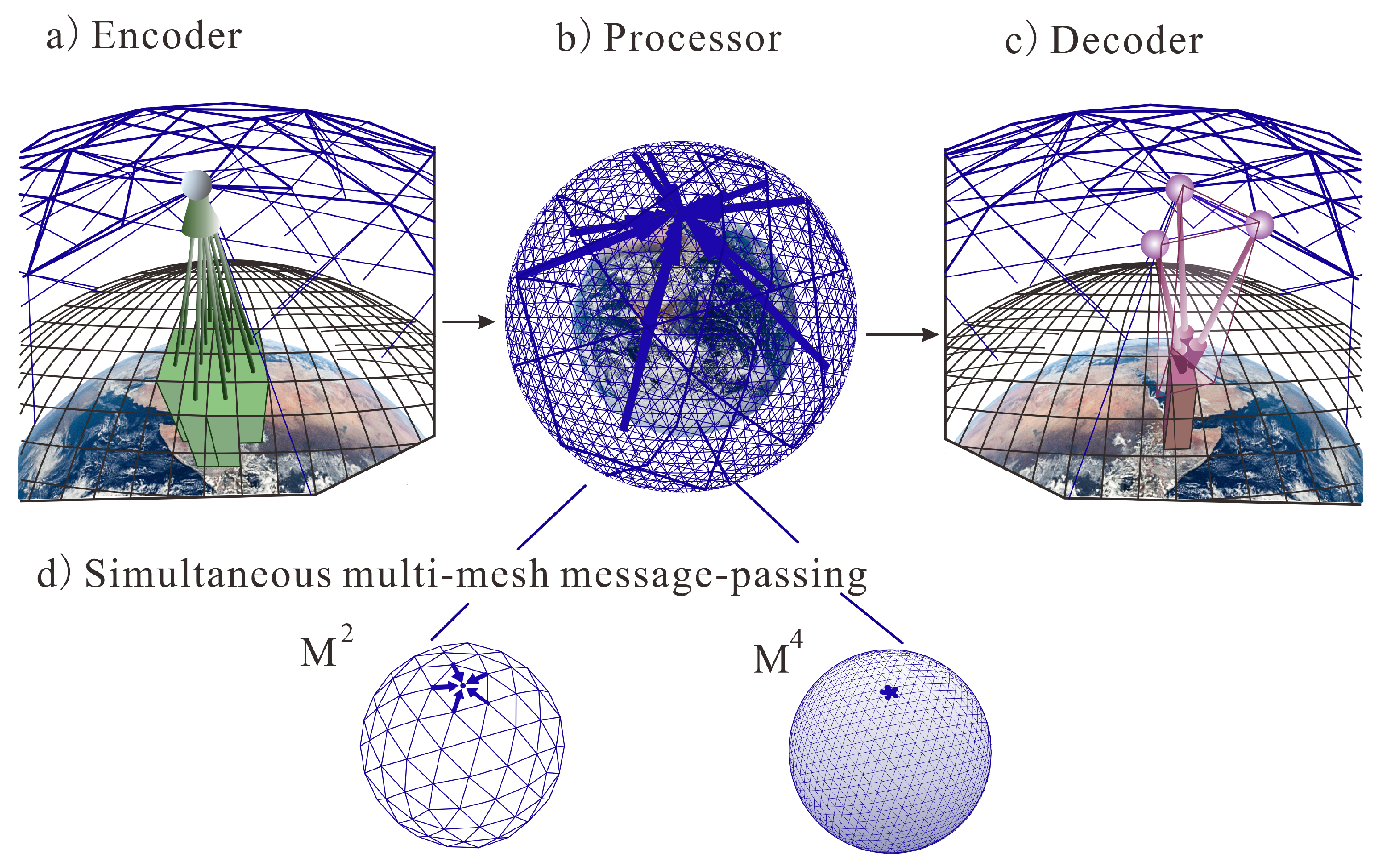
  • Encoder: The encoder component maps the local region of the input data (on the original latitude-longitude grid) onto the nodes of the multigrid graphical representation. It maps two consecutive input frames of the latitude-longitude input grid, with numerous variables per grid point, into a multi-scale internal mesh representation. This mapping process helps the model better capture and understand spatial dependencies in the data, allowing for more accurate predictions of future weather conditions.
  • Processor: This part performs several rounds of message-passing on the multi-mesh, where the edges can span short or long ranges, facilitating efficient communication without necessitating an explicit hierarchy. More specifically, the section uses a multi-mesh graph representation. It refers to a special graph structure that is able to represent the spatial structure of the Earth’s surface in an efficient way. In a multi-mesh graph representation, nodes may represent specific regions of the Earth’s surface, while edges may represent spatial relationships between these regions. In this way, models can capture spatial dependencies on a global scale and are able to utilize the power of GNNs to analyze and predict weather changes.
  • Decoder: It then maps the multi-mesh representation back to the latitude-longitude grid as a prediction for the next time step.
The workflow of GraphCast begins with the input of weather state(s) defined on a high-resolution latitude-longitude-pressure-levels grid. The encoder processes these inputs into a multi-scale internal mesh representation, which then undergoes many rounds of message-passing in the processor to capture spatio-temporal relationships in the weather data. Finally, the decoder translates the multi-mesh representation back to the latitude-longitude grid to generate predictions for subsequent time steps. It is worth noting that, as shown in the next part, due to the multi-scale mesh mapping property, the model is able to capture both localized weather features on a high-resolution mesh and large-scale weather features on a low-resolution mesh at the same time.
In essence, GraphCast encapsulates a pioneering stride in enhancing weather forecasting accuracy and efficiency through the amalgamation of machine learning and complex dynamical system modeling. It uniquely employs an autoregressive model structure underpinned by graph neural networks and a multi-scale mesh representation. The model’s “encode-process-decode” configuration, executed through a novel multi-mesh graphical representation, adeptly captures spatial dependencies and facilitates global-scale weather prediction. By processing high-resolution weather data inputs through a systematic workflow of encoding, message-passing, and decoding, GraphCast not only generates precise weather predictions for subsequent time intervals but also exemplifies the profound potential of machine learning in advancing meteorological forecasting methodologies.
PanGu. In the rapidly evolving field of meteorological forecasting, PanGu emerges as a pioneering model shown in Figure 5, predicated on a three-dimensional neural network that transcends traditional boundaries of latitude and longitude. Recognizing the intrinsic relationship between meteorological data and atmospheric pressure, PanGu incorporates a neural network structure that accounts for altitude in addition to latitude and longitude. The initiation of the PanGu model’s process involves Block Embedding, where the dataset is parsed into smaller subsets, or blocks. This operation not only mitigates spatial resolution and complexity but also facilitates subsequent data management within the network.
Following block embedding, the PanGu model integrates the data blocks into a 3D cube through a process known as 3D Cube Fusion, thereby enabling data processing within a tri-dimensional space. Swin Encoding [86], a specialized transformer encoder utilized in the deep learning spectrum, applies a self-attention mechanism for data comprehension and processing. This encoder, akin to the Autoencoder, excels at extracting and encoding essential information from the dataset. The ensuing phases include Decoding, which strives to unearth salient information, and Output Splitting, which partitions data into atmospheric and surface variables. Finally, Resolution Restoration reinstates the data to its original spatial resolution, making it amenable for further scrutiny and interpretation.
PanGu’s [49] innovative 3D neural network architecture [87] offers a groundbreaking perspective for integrating meteorological data, and its suitability for three-dimensional data is distinctly pronounced. Moreover, PanGu introduces a hierarchical time-aggregation strategy, an advancement that ensures the network with the maximum lead time is consistently invoked, thereby curtailing errors. In juxtaposition with running a model like FourCastNet [47] multiple times, which may accrue errors, this approach exhibits superiority in both speed and precision. Collectively, these novel attributes and methodological advancements position PanGu as a cutting-edge tool in the domain of high-resolution weather modeling, promising transformative potential in weather analysis and forecasting.
MetNet, FourCastNet, GraphCast, and PanGu are state-of-the-art methods in the field of weather prediction, and they share some architectural similarities that can indicate converging trends in this field. All four models initiate the process by embedding or downsampling the input data. FourCastNet uses AFNO, MetNet employs a Spatial Downsampler, and PanGu uses Block Embedding to manage the spatial resolution and complexity of the datasets, while GraphCast maps the input data from the original latitude-longitude grid into a multi-scale internal mesh representation. Spatio-temporal coding is an integral part of all networks; FourCastNet uses pre-training and fine-tuning phases to deal with temporal dependencies, MetNet uses ConvLSTM; PanGu introduces a hierarchical temporal aggregation strategy to manage temporal correlations in the data; and GraphCast employs GNNs to capture and address spatio-temporal dependencies in weather data. Each model employs a specialized approach to understand the spatial relationships within the data. FourCastNet uses AFNO along with Vision Transformers, MetNet utilizes Spatial Aggregator blocks, and PanGu integrates data into a 3D cube via 3D Cube Fusion, while GraphCast translates data into a multi-scale internal mesh. Both FourCastNet and PanGu employ self-attention mechanisms derived from the Transformer architecture for better capturing long-range dependencies in the data. FourCastNet combines FNO with ViT, and PanGu uses Swin Encoding.

5.2. Result Analysis

MetNet: According to the MetNet experiment, at the threshold of 1 mm/h precipitation rate, both MetNet and NWP predictions have high similarity to ground conditions. Evidently, MetNet exhibits a forecasting capability that is commensurate with NWP, distinguished by an accelerated computational proficiency that generally surpasses NWP’s processing speed.
FourCastNet: According to the FourCastNet experiment, FourCastNet can predict wind speed 96 h in advance with extremely high fidelity and accurate fine-scale features. In the experiment, the FourCastNet forecast accurately captured the formation and path of the super typhoon Shanzhu, as well as its intensity and trajectory over four days. It also has a high resolution and demonstrates excellent skills in capturing small-scale features. Particularly noteworthy is the performance of FourcastNet in forecasting meteorological phenomena within a 48 h horizon, which has transcended the predictive accuracy intrinsic to conventional numerical weather forecasting methodologies. This constitutes a significant stride in enhancing the veracity and responsiveness of short-term meteorological projections.
GraphCast: According to the GraphCast experiment, GraphCast demonstrates superior performance in tracking weather patterns, substantially outperforming NWP in various forecasting horizons, notably from 18 h to 4.75 days, as depicted in Figure 3b. It excels at predicting atmospheric river behaviors and extreme climatic events, with significant improvement seen in longer-term forecasts of 5 and 10 days. The model’s prowess extends to accurately capturing extreme heat and cold anomalies, showcasing not just its forecasting capability but a nuanced understanding of meteorological dynamics, thereby holding promise for more precise weather predictions with contemporary data.
PanGu: According to the PanGu experiment, PanGu can almost accurately predict typhoon trajectories during the tracking of strong tropical cyclones Kong Lei and Yu Tu and is 48 h faster than NWP. The advent of 3D Net further heralds a momentous advancement in weather prediction technology. This cutting-edge model outperforms numerical weather prediction models by a substantial margin and possesses the unprecedented ability to replicate reality with exceptional fidelity. It’s not merely a forecasting tool but a near-precise reflection of meteorological dynamics, allowing for a nearly flawless reconstruction of real-world weather scenarios.
In Table 3, “forecast-timeliness” represents the forecasting horizon of each model, indicating their ability to predict weather up to certain future days. In meteorology, z500 refers to the height at the 500 hPa isobaric level, which is critical for understanding atmospheric structures and weather systems. Model evaluation often employs RMSE (Root Mean Square Error) and ACC (Anomaly Correlation Coefficient) to gauge prediction accuracy and correlation with actual observations. Lower RMSE and higher ACC values indicate better model performance. Among GraphCast, PanGu, and IFS, PanGu exhibits the highest accuracy with an ACC of 0.872 for a 7-day forecast timeliness. GraphCast, while having a longer forecast timeliness of 9.75 days, has an ACC of 0.825 and an RMSE of 460, showing a balance between a longer forecasting duration and decent accuracy. Apart from this, introducing GPU data and prediction speed can provide crucial reference information for model selection, especially in scenarios with limited resources or where rapid responses are required. This aids in finding a balance between efficiency and effectiveness, offering support for successful forecasting.

6. Medium-to-Long-Term Climate Prediction

Medium-to-long-term climate predictions are usually measured in decadal quarters. In the domain of medium-to-long-term climate forecasting, the focal point extends beyond immediate meteorological events to embrace broader, macroscopic elements such as long-term climate change trends, average temperature fluctuations, and mean precipitation levels. This orientation is critical for a wide array of sectors, spanning from environmental policy planning to infrastructure development and agricultural projections. Over time, the forecasting methodologies have experienced significant advancements, evolving from conventional climate models to cutting-edge, computational methods such as Probabilistic Deep Learning for Climate Forecasting (CGF), Machine Learning for Model Down-scaling (DeepESD), and Machine Learning for Result Bias Correction (CycleGAN).

6.1. Model Design

Climate Model. Climate models, consisting of fundamental atmospheric dynamics and thermodynamic equations, focus on simulating Earth’s long-term climate system [89]. Unlike NWP, which targets short-term weather patterns, climate models address broader climatic trends. These models encompass Global Climate Models (GCMs), which provide a global perspective but often at a lower resolution, and Regional Climate Models (RCMs), designed for detailed regional analysis [90]. The main emphasis is on the average state and variations rather than transient weather events. The workflow of climate modeling begins with initialization by setting boundary conditions, possibly involving centuries of historical data. Numerical integration follows, using the basic equations to model the long-term evolution of the climate system [91]. Parameterization techniques are employed to represent sub-grid-scale processes like cloud formation and vegetation feedback. The model’s performance and uncertainties are then analyzed and validated by comparing them with observational data or other model results [92]. The advantages of climate models lie in their ability to simulate complex climate systems, providing forecasts and insights into future climate changes, thereby informing policy and adaptation strategies. However, they also present challenges such as high computational demands, sensitivity to boundary conditions, and potential uncertainties introduced through parameterization schemes. The distinction between GCMs and RCMs and their integration in understanding both global and regional climate phenomena underscores the sophistication and indispensable role of these models in advancing meteorological studies [93].
Conditional Generative Forecasting [61]. In the intricate arena of medium-to-long-term seasonal climate prediction, the scarcity of substantial datasets since 1979 poses a significant constraint on the rigorous training of complex models like CNNs, thus limiting their predictive efficacy. To navigate this challenge, a pioneering approach to transfer learning has been embraced, leveraging the simulated climate data drawn from CMIP5 (Coupled Model Intercomparison Project Phase 5) [94] to enhance modeling efficiency and accuracy. The process begins with a pre-training phase, where the CNN is enriched with CMIP5 data to comprehend essential climatic patterns and relationships. This foundational insight then transfers seamlessly to observational data without resetting the model parameters, ensuring a continuous learning trajectory that marries simulated wisdom with empirical climate dynamics. The methodology culminates in a fine-tuning phase, during which the model undergoes subtle refinements to align more closely with the real-world intricacies of medium-to-long-term ENSO forecasting [18]. This innovative strategy demonstrates the transformative power of transfer learning in addressing the formidable challenges associated with limited sample sizes in medium-to-long-term climate science.
Leveraging 52,201 years of climate simulation data from CMIP5/CMIP6, which serves to increase the sample size, the method for medium-term forecasting employs CNNs and Temporal Convolutional Neural Networks (TCNNs) to extract essential features from high-dimensional geospatial data. This feature extraction lays the foundation for probabilistic deep learning, which determines an approximate distribution of the target variables, capturing the data’s structure and uncertainty [95]. The model’s parameters are optimized by maximizing the Evidence Lower Bound (ELBO) within the variational inference framework. The structure is shown in Figure 6. The integration of deep learning techniques with probabilistic modeling ensures accuracy, robustness to sparse data, and flexibility in assumptions, enhancing the precision of forecasts and offering valuable insights into confidence levels and expert knowledge integration.
Leveraging advanced techniques in variational inference and neural networks, the method described seeks to approximate the complex distribution p ( Y X , M ) , where Y is the target variable and X and M are predictor and GCM index information, respectively. The process is outlined as follows:
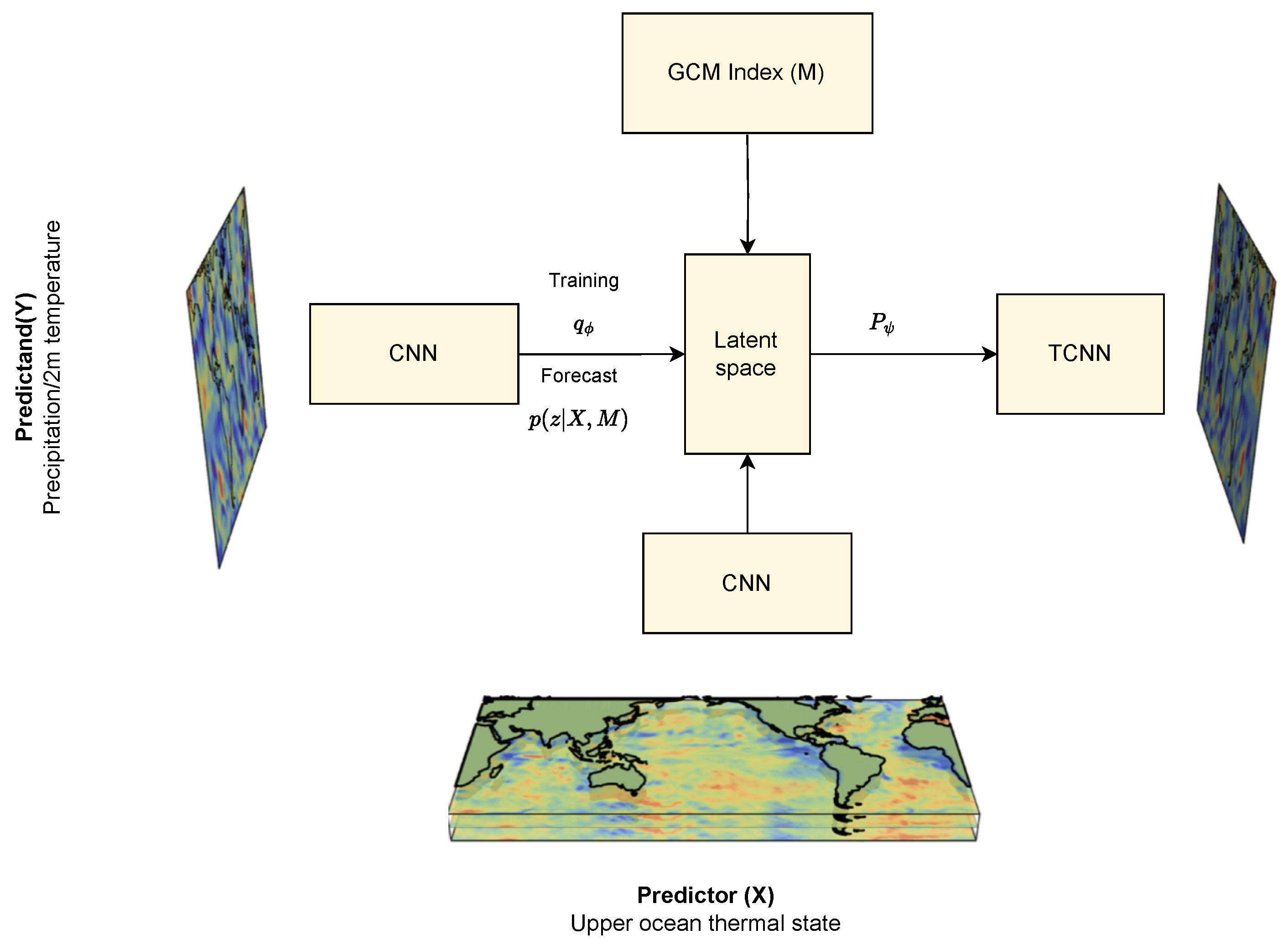
  • Problem Definition: The goal is to approximate p ( Y X , M ) , a task challenged by high-dimensional geospatial data, data inhomogeneity, and a large dataset.
  • Model Specification:
    • Random Variable z: A latent variable with a fixed standard Gaussian distribution.
    • Parametric Functions p θ , q ϕ , p ψ : Neural networks for transforming z and approximating target and posterior distributions.
    • Objective Function: Maximization of the Evidence Lower Bound (ELBO).
  • Training Procedure:
    • Initialize: Define random variable z N ( 0 , 1 ) [96,97]
      parametric functions p θ ( z , X , M ) , q ϕ ( z X , Y , M ) , p ψ ( Y X , M , z ) .
    • Training Objective (Maximize ELBO) [98]: The ELBO is defined as:
      ELBO = E z q ϕ log p ψ ( Y X , M , z ) D KL ( q ϕ p ( z X , M ) ) D KL ( q ϕ p ( z X , Y , M ) )
      with terms for reconstruction, regularization, and residual error.
    • Optimization: Utilize variational inference, Monte Carlo reparameterization, and Gaussian assumptions.
  • Forecasting: Generate forecasts by sampling p ( z X , M ) , the likelihood of p ψ , and using the mean of p ψ for an average estimate.
This method embodies a rigorous approach to approximating complex distributions, bridging deep learning and probabilistic modeling to enhance forecasting accuracy and insights.
ELBO ( λ ) = E q ( z | x ) log p ( x , z ) log q ( z | x ) ( Evidence Lower Bound )
In summary, the combination of deep learning and probabilistic insights presents a unique and potent method for spatial predictive analytics. The approach is marked by scalability, flexibility, and an ability to learn complex spatial features, even though challenges persist, such as intrinsic complexity in computational modeling and the requirement for a profound statistical and computer science background. Its potential in handling large data sets and adapting to varying scenarios highlights its promising applicability in modern spatial predictive analytics, representing an advanced tool in the arena of seasonal climate prediction.
Cycle-Consistent Generative Adversarial Networks. Cycle-Consistent Generative Adversarial Networks (CycleGANs) have been ingeniously applied to the bias correction of high-resolution Earth System Model (ESM) precipitation fields, such as GFDL-ESM4 [99]. This model includes two generators responsible for translating between simulated and real domains, and two discriminators to differentiate between generated and real observations. A key component of this approach is the cycle consistency loss, which ensures a reliable translation between domains coupled with a constraint to maintain global precipitation values for physical consistency. By framing bias correction as an image-to-image translation task, CycleGANs have significantly improved spatial patterns and distributions in climate projections. The model’s utilization of spatial spectral densities and fractal dimension measurements further emphasizes its spatial context awareness, making it a groundbreaking technique in the field of climate science. The CycleGAN model consists of two generators and two discriminators, along with a cycle consistency loss:
  • Two Generators: The CycleGAN model includes two generators. Generator G learns the mapping from the simulated domain to the real domain, and generator F learns the mapping from the real domain to the simulated domain [100].
  • Two Discriminators: There are two discriminators, one for the real domain and one for the simulated domain. Discriminator D x encourages generator G to generate samples that look similar to samples in the real domain, and discriminator D y encourages generator F to generate samples that look similar to samples in the simulated domain.
  • Cycle Consistency Loss: To ensure that the mappings are consistent, the model enforces the following condition through a cycle consistency loss: if a sample is mapped from the simulated domain to the real domain and then mapped back to the simulated domain, it should get a sample similar to the original simulated sample. Similarly, if a sample is mapped from the real domain to the simulated domain and then mapped back to the real domain, it should get a sample similar to the original real sample.
    L cyc ( G , F ) = E x p data ( x ) | | F ( G ( x ) ) x | | 1 + E y p data ( y ) | | G ( F ( y ) ) y | | 1
  • Training Process: The model is trained to learn the mapping between these two domains by minimizing the adversarial loss and cycle consistency loss between the generators and discriminators.
    L Gen ( G , F ) = L GAN ( G , D y , X , Y ) + L GAN ( F , D x , Y , X ) + λ L cyc ( G , F )
  • Application to Prediction: Once trained, these mappings can be used for various tasks, such as transforming simulated precipitation data into forecasts that resemble observed data.
The bidirectional mapping strategy of Cycle-Consistent Generative Adversarial Networks (CycleGANs) permits the exploration and learning of complex transformation relationships between two domains without reliance on paired training samples. This attribute holds profound significance, especially in scenarios where only unlabeled data are available for training. In its specific application within climate science, this characteristic of CycleGAN enables precise capturing and modeling of the subtle relationships between real and simulated precipitation data. Through this unique bidirectional mapping shown in Figure 7, the model not only enhances the understanding of climatic phenomena but also improves the predictive accuracy of future precipitation trends. This provides a novel, data-driven methodology for climate prediction and analysis, contributing to the ever-expanding field of computational climate science.
DeepESD. Traditional GCMs, while proficient in simulating large-scale global climatic dynamics [101,102], exhibit intrinsic limitations in representing finer spatial scales and specific regional characteristics. This inadequacy manifests as a pronounced resolution gap at localized scales, restricting the applicability of GCMs in detailed regional climate studies [103,104].
In stark contrast, the utilization of CNNs symbolizes a significant breakthrough [105]. Structurally characterized by hierarchical convolutional layers, CNNs possess the unique ability to articulate complex multi-scale spatial features across disparate scales, commencing with global coarse-grained characteristics and progressively refining to capture intricate regional details. An exemplar implementation of this approach was demonstrated by Baño-Medina et al. [104], wherein a CNN comprised three convolutional layers with spatial kernels of varying counts (50, 25, and 10, respectively). The transformation process began with the recalibration of ERA-Interim reanalysis data to a 2° regular grid, elevating it to 0.5° [106,107,108]. This configuration allowed the CNN to translate global atmospheric patterns into high-resolution regional specificity [109,110].
The nuanced translation from global to regional scales, achieved through sequential convolutional layers, not only amplifies the spatial resolution but also retains the contextual relevance of climatic variables [111,112]. The first convolutional layer captured global coarse-grained features, with subsequent layers incrementally refining these into nuanced regional characteristics. By the terminal layer, the CNN had effectively distilled complex atmospheric dynamics into a precise, high-resolution grid [113,114].
This enhancement fosters a more robust understanding of regional climatic processes, ushering in an era of precision and flexibility in climate modeling. The deployment of this technology affirms a pivotal advancement in the field, opening new possibilities for more granulated, precise, and comprehensive examination of climatic processes and future scenarios [115,116,117]. The introduction of CNNs thus represents a transformative approach shown in Figure 8 to bridging the resolution gap inherent to traditional GCMs, with substantial implications for future climate analysis and scenario planning.
NNCAM. The design and implementation of the Neural Network Community Atmosphere Model (NNCAM) are architected to leverage advancements in machine learning for improved atmospheric simulations. The architecture is a nuanced blend of traditional General Circulation Models (GCMs), specifically the Super-Parameterized Community Atmosphere Model (SPCAM), and cutting-edge machine learning techniques like Residual Deep Neural Networks (ResDNNs).
  • Reference Model: SPCAM. SPCAM serves as the foundational GCM and is embedded with Cloud-Resolving Models (CRMs) to simulate microscale atmospheric processes like cloud formation and convection. SPCAM is employed to generate “target simulation data”, which serves as the training baseline for the neural networks. The use of CRMs is inspired by recent advancements in data science, demonstrating that machine learning parameterizations can potentially outperform traditional methods in simulating convective and cloud processes.
  • Neural Networks: ResDNNs, a specialized form of deep neural networks, are employed for their ability to approximate complex, nonlinear relationships. The network comprises multiple residual blocks, each containing two fully connected layers with Rectified Linear Unit (ReLU) activations. ResDNNs are designed to address the vanishing and exploding gradient problems in deep networks through residual connections, offering a stable and effective gradient propagation mechanism. This makes them well-suited for capturing the complex and nonlinear nature of atmospheric processes.
  • Subgrid-Scale Physical Simulator. Traditional parameterizations often employ simplified equations to model subgrid-scale processes, which might lack accuracy. In contrast, the ResDNNs are organized into a subgrid-scale physical simulator that operates independently within each model grid cell. This simulator takes atmospheric states as inputs and outputs physical quantities at the subgrid scale, such as cloud fraction and precipitation rate.
In the NNCAM model, the core workflow is divided into several key steps to achieve efficient and accurate climate simulations. First, the dynamic core, which serves as the base component of the model, is responsible for solving the underlying hydrodynamic equations and calculating the current climate state, e.g., temperature, pressure, and humidity, as well as the environmental forcings, e.g., wind and solar radiation. These calculations are then transmitted to the NN-GCM coupler. Upon receiving these data, the coupler further passes them to the neural network parameterization module. This module utilizes pre-trained neural networks, specifically ResDNNs, for faster and more accurate parameterization of the climate. Upon completion of the predictions, these results are fed back to the host GCM, i.e., NNCAM. The host GCM then uses the predictions generated by these neural networks to update the climate state in the model, and based on these updates, it performs the simulation at the next time step.
Overall, the host GCM, as the core of the whole simulation, is not only responsible for the basic climate simulation but also efficiently interacts with the dynamic core and neural network parameterization modules to achieve higher simulation accuracy and computational efficiency. This hierarchical architecture ensures both computational efficiency and high simulation fidelity. It allows for seamless integration and synchronization of the model states and predictions, thereby enabling continuous and efficient operation of NNCAM. The proposed framework represents a significant stride in the realm of atmospheric science, offering a harmonious integration of machine learning and physical simulations to achieve unprecedented accuracy and computational efficiency.
CGF, DeepESD, and CycleGAN are very different in their uses and implementations, but there are also some levels of similarity. All three approaches focus on mapping from one data distribution to another. Furthermore, they focus more on the mechanisms of climate change than previous models for weather forecasting. CycleGAN specifically emphasizes the importance of not only mapping from distribution A to B but also the inverse mapping capability from B to A, which is to some extent what CGF and DeepESD are concerned with. NNCAM realizes the mapping from physical parameterization to machine learning parameterization. This mapping can be viewed as a functional mapping that replaces parameterized functions in the physical process with functions learned and inferred by the machine learning model.

6.2. Result Analysis

CGF: In the utilization of deep probabilistic machine learning techniques, the figure compares the performance of the CGF model using both simulated samples and actual data against the traditional climate model, Cancm4. The findings illustrate that our model outperforms the conventional climate modeling approach in terms of accuracy, irrespective of the employment of simulated or real data sets. This distinction emphasizes the enhanced predictive capability of our method and underlines its potential superiority in handling complex meteorological phenomena.
CycleGANs: In the context of long-term climate estimation, the application of deep learning for model correction has yielded promising results. As illustrated in the accompanying figure, the diagram delineates the mean absolute errors of different models relative to the W5E5v2 baseline facts. Among these, the error correction technique utilizing Generative Adversarial Networks (GANs) in conjunction with the ISIMIP3BASD physical model has demonstrated the lowest discrepancy. This evidence underscores the efficacy of sophisticated deep-learning methodologies in enhancing the precision of long-term climate estimations, thereby reinforcing their potential utility in climatological research and forecasting applications.
DeepESD: In the conducted study, deep learning has been employed to enhance resolution, resulting in a model referred to as DeepESD. The following figure portrays the Probability Density Functions (PDFs) of precipitation and temperature for the historical period from 1979 to 2005, as expressed by the General Circulation Model (GCM) in red, the Regional Climate Model (RCM) in blue, and DeepESD in green. These are contextualized across regions such as the Alps, the Iberian Peninsula, and Eastern Europe as defined by the PRUDENCE area. In the diagram, solid lines represent the overall mean, while the shaded region includes two standard deviations. Dashed lines depict the distribution mean of each PDF. A clear observation from the graph illustrates that DeepESD maintains higher consistency with observed data in comparison to the other models.
NNCAM: NNCAM has demonstrated proficient simulation of strong precipitation centers across maritime continental tropical regions, Asian monsoon areas, South America, and the Caribbean. The model maintains the spatial pattern and global average of precipitation over the subsequent 5 years in its simulation, showcasing its long-term stability. Overall, in terms of the spatial distribution of multi-annual summer precipitation, NNCAM results are closer to the standard values compared with those from CAM5, with smaller root mean square errors and global average deviations. Additionally, NNCAM operates at a speed that is 30 times faster than traditional models, marking a significant stride in enhancing computational efficiency.
In Table 4, MAE is a metric commonly used to measure the magnitude of forecast errors. It calculates the average of the absolute errors between the actual and predicted values. This metric was selected because it provides a clear, intuitive way to understand the accuracy of model predictions. A low MAE value indicates better prediction accuracy, while a high MAE value indicates a larger prediction error. The Euclidean Distance to Observations in the Probability Density Function (PDF) is utilized to evaluate the performance of the model by comparing the distance difference in the PDFs between the predicted and actual observed data. This metric was selected because it provides a means of quantifying how well a model’s predicted distribution aligns with the actual observed distribution, enabling the evaluation of model performance in complex systems, particularly when dealing with systems that possess inherent uncertainty and variability. While these four methods address different problems and, thus, a direct comparison is not feasible in this study, it is evident that they all exhibit significant improvements compared with traditional earth system models.
From the results, it can be discerned that although the utilization of machine learning has significantly diminished in medium-to-long-term climate forecasting, our findings demonstrate that by judiciously addressing the challenge of scarce sample sizes and employing appropriate machine learning techniques, superior results can still be achieved compared with those derived from physical models. This observation underscores the potential of machine learning methodologies to enhance prediction accuracy in climate science, even in situations constrained by data limitations. In the context of climate estimation, it is observable that the utilization of neural networks for predicting climate variations has become less prevalent among meteorologists. However, the adoption of machine learning techniques to aid and optimize climate modeling has emerged as a complementary strategy. As evidenced by the two preceding figures, climate models that have been enhanced through the application of machine learning demonstrate superior predictive capabilities when compared with other conventional models.

7. Discussion

Weather forecasting and climate prediction are closely related to people’s lives and provide important information and support for social and economic activities. For example, governments and relief organizations rely on accurate weather forecasts to warn of and respond to natural disasters, thereby mitigating their impact on people’s lives and property. At the same time, the energy industry also relies heavily on climate forecasts to predict energy demand and optimize energy distribution, thereby ensuring the stability and efficiency of energy supply. Our research purpose, the examination of machine learning in meteorological forecasting, is situated within a rich historical context, charting the evolution of weather prediction methodologies. Starting from simple statistical methods to complex deterministic modeling, the field has witnessed a paradigm shift with the advent of machine learning techniques.

7.1. Overall Comparison

In this section of our survey, we delineate key differences between our study and existing surveys, thereby underscoring the unique contribution of our work. We contrast various time scales—short-term versus medium-to-long-term climate predictions—to substantiate our rationale for focusing on these particular temporal dimensions. Additionally, we draw a comparative analysis between machine learning approaches and traditional models in climate prediction. This serves to highlight our reason for centering our survey on machine learning techniques for climate forecasting. Overall, this section not only amplifies the distinctiveness and relevance of our survey but also frames it within the larger scientific discourse.
Comparison to existing surveys. Compared to existing literature, our survey takes a unique approach by cohesively integrating both short-term weather forecasting and medium-to-long-term climate predictions—a dimension often underrepresented. While other surveys may concentrate on a limited range of machine learning methods, ours extends to nearly 20 different techniques. However, we recognize our limitations, particularly the challenge of providing an exhaustive analysis due to the complexity of machine learning algorithms and their multifaceted applications in meteorology. This signals an opportunity for future research to delve deeper into specialized machine-learning techniques or specific climatic variables. In contrast to many generalized surveys, our study ventures into the technical nuances of scalability, interpretability, and applicability for each method. We also make a conscious effort to incorporate the most recent advances in the field, although we acknowledge that the pace of technological change inevitably leaves room for further updates. In sum, while our survey provides a more comprehensive and technically detailed roadmap than many existing reviews, it also highlights gaps and opportunities for future work in this rapidly evolving interdisciplinary domain.
Short-term weather prediction vs. medium-to-long-term climate predication. Short-term weather predictions focus on immediate atmospheric conditions within a time span of hours to days. This is a contrast to medium-to-long-term climate predictions, which aim to forecast broader patterns in weather, temperature trends, and precipitation averages over extended timeframes of months to decades. The goals underlying these two forms of prediction also diverge significantly. Short-term forecasts are usually operational in nature, aimed at immediate public safety or aiding sectors like agriculture and industry, whereas medium-to-long-term predictions typically inform strategic and policy-oriented planning for various societal sectors, including agriculture, energy, and urban development.
This comparison extends to the variables considered in the predictive models. Short-term weather predictions often hone in on localized states like temperature, humidity, wind speed, and precipitation. On the other hand, medium-to-long-term climate predictions scrutinize a wider array of variables, such as average temperature shifts, sea-level rise, and the general patterns of extreme weather events, often on a global or regional scale.
Regarding methodologies, machine learning techniques such as neural networks, random forests, and support vector machines are frequently deployed in the realm of short-term weather prediction, owing to their prowess in swiftly analyzing large datasets. In contrast, for medium-to-long-term climate predictions, machine learning generally complements traditional physics-based models, serving a supplementary role to handle the complexities and uncertainties inherent in longer-range forecasts.
Finally, each type of prediction comes with its own set of challenges. Short-term forecasts grapple with issues related to the accuracy and granularity of the data and the speed of its dissemination to the public. Medium-to-long-term climate predictions, however, face challenges related to the scarcity of quality long-term datasets and the intricacies associated with interdependent climatic variables. Yet, there are challenges that are common to both, exemplified by the nonlinearity inherent in weather and climate prediction models, which underscore the complex dynamic relationships among atmospheric variables, necessitating techniques adept at capturing such intricate interactions. Furthermore, the assessment of model uncertainties is arduous as they emanate from various facets, demanding algorithms that can quantify, accommodate, and ideally mitigate these uncertainties to augment the reliability and accuracy of predictions.
Machine-learning models vs. traditional models. In terms of computational speed, machine learning algorithms—particularly those based on deep learning—have the capability to process extensive datasets at a far quicker rate compared with traditional methodologies. When it comes to prediction accuracy, the machine learning algorithms stand out for their superior feature extraction capabilities, often yielding more precise outcomes in short-term weather forecasting scenarios. Additionally, the adaptability of machine learning models enables them to evolve and improve over time. This flexibility makes them particularly useful tools that can be fine-tuned as climate data and observational technologies continue to advance.
While machine learning models can excel at generating rapid and sometimes more accurate forecasts, their lack of interpretability can be a barrier to gaining deeper scientific insights. Machine learning models, especially complex ones like deep neural networks, are often considered “black boxes”, meaning their internal workings are not easily understandable. This is a significant drawback during meteorological application. Understanding the underlying mechanisms of weather and climate variability is crucial across all temporal scales, serving as the bedrock upon which all predictive methods are built. For instance, in short-term weather forecasting, an in-depth grasp of these mechanisms assists researchers in selecting the most relevant datasets. For example, when forecasting precipitation, it would be ineffective to merely input precipitation data as a training set. Instead, one must understand the specific meteorological factors that influence precipitation in a given region. This necessity becomes even more pronounced for medium-to-long-term forecasts, which are inherently more complex. To construct accurate and reliable models, it is imperative to identify the factors that interact with each other, eventually leading to variations in the target predictive elements for a particular region. Thus, a nuanced understanding of these mechanisms not only enhances the precision of our models but also broadens the scope for comprehensive climatic analysis and future scenario planning.

7.2. Challenge

Although we found extensive work on machine learning frameworks that succeed in short-term weather prediction and even outperform traditional methods, climate prediction in the medium-to-long term mainly relies on traditional methods. The main challenges can be attributed to the limited data size and complex climate change effects.
Dataset. The scarcity of seasonal meteorological data, particularly evident from the era around 1979, poses significant challenges for applying machine learning to climate prediction. While data from this period may be adequate for short-term weather forecasting, it falls short for medium-to-long-term climate models. This data limitation impacts machine learning algorithms, which rely on large, quality datasets for robust training. Consequently, the lack of seasonal data affects not only the model’s performance and reliability but also complicates validation procedures. This makes it challenging to assess the model’s generalizability and accuracy. Additionally, the sparse data hampers the effective fusion of machine learning with traditional physics-based models, affecting the overall reliability of climate predictions. Therefore, the limitations of historical meteorological data significantly constrain the application of machine learning in long-term climate studies.
Complex climate change effect. A certain climate change may be related to hundreds or thousands of variables. It’s difficult for us to use machine learning to capture their correlation. The intricate nature of climate change, influenced by hundreds or even thousands of interrelated variables, presents a daunting challenge for machine learning applications in climate prediction. Unlike simpler systems, where causal relationships between variables are straightforward, climate systems embody complex, non-linear interactions that are difficult to model. Machine learning algorithms, though powerful, often require clearly defined feature sets and labels for effective training, a condition seldom met in the realm of climate science. The sheer number of variables can lead to issues of dimensionality, where the complexity of the model grows exponentially, making it computationally intensive and difficult to interpret. Furthermore, capturing long-term dependencies between these myriad variables is particularly challenging, given the current state-of-the-art in machine learning techniques. This complexity often results in models that, while mathematically sophisticated, lack the interpretability necessary for scientific validation and policy implications.

7.3. Future Work

For these challenges and the disadvantages of machine-learning prediction methods in meteorology, we propose the following future work:
  • Simulate the dataset using statistical methods or physical methods.
  • Combining statistical knowledge with machine learning methods to enhance the interpretability of patterns.
  • Consider the introduction of physics-based constraints into deep learning models to produced more accurate and reliable results.
  • Accelerating Physical Model Prediction with machine learning knowledge.
Simulating Datasets: One promising avenue for future work is to simulate datasets using either statistical or physical methods. Such synthetic datasets can provide a controlled environment to test and validate predictive models. Utilizing methods like Monte Carlo simulations or employing first-principle equations to generate realistic data, this approach promises to enhance model robustness by enabling better generalizability testing.
Enhancing Interpretability: The issue of interpretability is a well-known drawback of machine learning models. A future research direction could be the fusion of statistical methodologies with machine learning algorithms. Incorporating statistical tests for feature selection or Bayesian methods for uncertainty quantification can render the inherently opaque machine learning models more interpretable, thereby making their results more actionable in critical fields like meteorology.
Physics-Based Constraints: A particularly vital frontier for research is the integration of atmospheric physics-based constraints into deep learning architectures. Traditional machine learning models, when unconstrained, might produce forecasts that, although statistically plausible, violate fundamental principles of atmospheric physics and dynamics. To mitigate this, it would be beneficial to incorporate terms or constraints that reflect the known interactions among meteorological elements such as temperature, pressure, and humidity. This can be done through methods like Physics-Informed Neural Networks (PINNs) or physics-based regularization terms. Such an approach would be invaluable for complex meteorological applications like severe weather forecasting, where both the accuracy and physical plausibility of predictions are of utmost importance.
Accelerating Physical Models: Lastly, the intersection of machine learning with traditional physical models offers significant potential. Physical models are often computationally intensive; however, machine learning can expedite these calculations. Techniques such as model parallelization or simpler surrogate models developed via machine learning could dramatically speed up real-time analysis and forecasting, a critical need in time-sensitive applications.
Machine Learning (ML), a subset of Artificial Intelligence (AI), holds a distinctive prowess in discerning patterns from large datasets, yet it does not possess the capability to replace physical models, including the NWP and the Global Climate Model. This limitation predominantly stems from ML’s inherent “black box” nature, which lacks explicability, in contrast to the physical models based on atmosphere principles. The symbiotic alliance between ML and physical models unveils a plethora of enhancements in weather forecasting. Specifically, ML significantly augments physical models in areas like bias correction, parameterization, and Down-scaling, where the fusion of data-driven insights with physical models tends to yield more accurate and efficient forecasts. On the flip side, physical models enrich ML by imparting robust physical constraints that guide the learning process towards physically plausible solutions. The inextricable synergy between ML and NWP models is underscored by their irreplaceable strengths, heralding a future where their collaborative integration could unlock new horizons in advancing meteorological science and forecasting accuracy. This harmonious coexistence not only propels the forecasting capabilities to new heights but also bridges the interpretability gap, thereby fostering a more comprehensive understanding and enhanced trust in predictive modeling within the meteorological community.

8. Conclusions

In conclusion, this study offers an extensive look into the transformative role of machine learning in meteorological forecasting. It uniquely amalgamates short-term weather forecasting with medium- and long-term climate predictions, covering a total of 20 models and providing an in-depth introduction to eight select models that stand at the forefront of the industry. Our rigorous survey helps distinguish the operational mechanisms of these eight models, serving as a reference for model selection in various contexts. Furthermore, this work identifies current challenges, like the limited dataset of chronological seasons, and suggests future research directions, including data simulation and the incorporation of physics-based constraints. Thus, the survey not only provides a comprehensive current view but also outlines a roadmap for future interdisciplinary work in this burgeoning field. While the research acknowledges its limitations in providing an exhaustive analysis, it delineates a promising direction for future exploration.

Author Contributions

Conceptualization, L.C., Z.Y. and B.H.; methodology, L.C. and Z.Y.; validation, L.C., Z.Y., B.H., J.Z. and X.W.; formal Analysis, Z.Y., L.C., B.H. and W.Y.; resources, J.Z. and L.C.; data curation, L.C. and B.H.; writing—original draft preparation, L.C.; writing—review & editing, L.C., Z.Y. and B.H.; proof reading L.C., Z.Y., B.H., X.W., J.Z. and W.Y.; supervision, Z.Y., X.W. and J.Z.; project administration, Z.Y. and X.W.; funding acquisition, Z.Y. and X.W. All authors have read and agreed to the published version of the manuscript.

Funding

This research received no external funding.

Institutional Review Board Statement

Not applicable.

Informed Consent Statement

Not applicable.

Data Availability Statement

Not applicable.

Conflicts of Interest

The authors declare no conflict of interest.

Abbreviations

Commonly used symbols and definitions:
SymbolDefinition
vvelocity vector
ttime
ρ fluid density
ppressure
μ dynamic viscosity
ggravitational acceleration vector
E q ( z | x ) expectation under the variational distribution q ( z | x )
z latent variable
x observed data
p ( x , z ) joint distribution of observed and latent variables
q ( z | x ) variational distribution
G, FGenerators for mappings from simulated to real domain and vice versa.
D x , D y Discriminators for real and simulated domains.
L cyc , L GAN Cycle consistency loss and Generative Adversarial Network loss.
X, YData distributions for simulated and real domains.
λ Weighting factor for the cycle consistency loss.

References

  1. Abbe, C. The physical basis of long-range weather. Mon. Weather Rev. 1901, 29, 551–561. [Google Scholar] [CrossRef]
  2. Zheng, Y.; Capra, L.; Wolfson, O.; Yang, H. Urban computing: Concepts, methodologies, and applications. Acm Trans. Intell. Syst. Technol. TIST 2014, 5, 1–55. [Google Scholar]
  3. Gneiting, T.; Raftery, A.E. Weather forecasting with ensemble methods. Science 2005, 310, 248–249. [Google Scholar] [CrossRef] [PubMed]
  4. Agapiou, A. Remote sensing heritage in a petabyte-scale: Satellite data and heritage Earth Engine applications. Int. J. Digit. Earth 2017, 10, 85–102. [Google Scholar] [CrossRef]
  5. Bendre, M.R.; Thool, R.C.; Thool, V.R. Big data in precision agriculture: Weather forecasting for future farming. In Proceedings of the 2015 1st International Conference on Next Generation Computing Technologies (NGCT), Dehradun, India, 4–5 September 2015; pp. 744–750. [Google Scholar]
  6. Zavala, V.M.; Constantinescu, E.M.; Krause, T. On-line economic optimization of energy systems using weather forecast information. J. Process Control 2009, 19, 1725–1736. [Google Scholar] [CrossRef]
  7. Nurmi, V.; Perrels, A.; Nurmi, P.; Michaelides, S.; Athanasatos, S.; Papadakis, M. Economic value of weather forecasts on transportation–Impacts of weather forecast quality developments to the economic effects of severe weather. EWENT FP7 Project. 2012, Volume 490. Available online: http://virtual.vtt.fi/virtual/ewent/Deliverables/D5/D5_2_16_02_2012_revised_final.pdf (accessed on 8 September 2023).
  8. Russo, J.A., Jr. The economic impact of weather on the construction industry of the United States. Bull. Am. Meteorol. Soc. 1966, 47, 967–972. [Google Scholar] [CrossRef]
  9. Badorf, F.; Hoberg, K. The impact of daily weather on retail sales: An empirical study in brick-and-mortar stores. J. Retail. Consum. Serv. 2020, 52, 101921. [Google Scholar] [CrossRef]
  10. De Freitas, C.R. Tourism climatology: Evaluating environmental information for decision making and business planning in the recreation and tourism sector. Int. J. Biometeorol. 2003, 48, 45–54. [Google Scholar] [CrossRef]
  11. Smith, K. Environmental Hazards: Assessing Risk and Reducing Disaster; Routledge: London, UK, 2013. [Google Scholar]
  12. Hammer, G.L.; Hansen, J.W.; Phillips, J.G.; Mjelde, J.W.; Hill, H.; Love, A.; Potgieter, A. Advances in application of climate prediction in agriculture. Agric. Syst. 2001, 70, 515–553. [Google Scholar] [CrossRef]
  13. Guedes, G.; Raad, R.; Raad, L. Welfare consequences of persistent climate prediction errors on insurance markets against natural hazards. Estud. Econ. Sao Paulo 2019, 49, 235–264. [Google Scholar] [CrossRef]
  14. McNamara, D.E.; Keeler, A. A coupled physical and economic model of the response of coastal real estate to climate risk. Nat. Clim. Chang. 2013, 3, 559–562. [Google Scholar] [CrossRef]
  15. Kleerekoper, L.; Esch, M.V.; Salcedo, T.B. How to make a city climate-proof, addressing the urban heat island effect. Resour. Conserv. Recycl. 2012, 64, 30–38. [Google Scholar] [CrossRef]
  16. Kaján, E.; Saarinen, J. Tourism, climate change and adaptation: A review. Curr. Issues Tour. 2013, 16, 167–195. [Google Scholar]
  17. Dessai, S.; Hulme, M.; Lempert, R.; Pielke, R., Jr. Climate prediction: A limit to adaptation. Adapt. Clim. Chang. Threshold. Values Gov. 2009, 64, 78. [Google Scholar]
  18. Ham, Y.-G.; Kim, J.-H.; Luo, J.-J. Deep Learning for Multi-Year ENSO Forecasts. Nature 2019, 573, 568–572. [Google Scholar] [CrossRef] [PubMed]
  19. Howe, L.; Wain, A. Predicting the Future; Cambridge University Press: Cambridge, UK, 1993; Volume V, pp. 1–195. [Google Scholar]
  20. Hantson, S.; Arneth, A.; Harrison, S.P.; Kelley, D.I.; Prentice, I.C.; Rabin, S.S.; Archibald, S.; Mouillot, F.; Arnold, S.R.; Artaxo, P.; et al. The status and challenge of global fire modelling. Biogeosciences 2016, 13, 3359–3375. [Google Scholar]
  21. Racah, E.; Beckham, C.; Maharaj, T.; Ebrahimi Kahou, S.; Prabhat, M.; Pal, C. ExtremeWeather: A large-scale climate dataset for semi-supervised detection, localization, and understanding of extreme weather events. Adv. Neural Inf. Process. Syst. 2017, 30, 3402–3413. [Google Scholar]
  22. Gao, S.; Zhao, P.; Pan, B.; Li, Y.; Zhou, M.; Xu, J.; Zhong, S.; Shi, Z. A nowcasting model for the prediction of typhoon tracks based on a long short term memory neural network. Acta Oceanol. Sin. 2018, 37, 8–12. [Google Scholar]
  23. Ren, X.; Li, X.; Ren, K.; Song, J.; Xu, Z.; Deng, K.; Wang, X. Deep Learning-Based Weather Prediction: A Survey. Big Data Res. 2021, 23, 100178. [Google Scholar]
  24. Reichstein, M.; Camps-Valls, G.; Stevens, B.; Jung, M.; Denzler, J.; Carvalhais, N.; Prabhat, F. Deep learning and process understanding for data-driven Earth system science. Nature 2019, 566, 195–204. [Google Scholar] [CrossRef]
  25. Stockhause, M.; Lautenschlager, M. CMIP6 data citation of evolving data. Data Sci. J. 2017, 16, 30. [Google Scholar] [CrossRef]
  26. Hsieh, W.W. Machine Learning Methods in the Environmental Sciences: Neural Networks and Kernels; Cambridge University Press: Cambridge, UK, 2009. [Google Scholar]
  27. Krasnopolsky, V.M.; Fox-Rabinovitz, M.S.; Chalikov, D.V. New Approach to Calculation of Atmospheric Model Physics: Accurate and Fast Neural Network Emulation of Longwave Radiation in a Climate Model. Mon. Weather Rev. 2005, 133, 1370–1383. [Google Scholar] [CrossRef]
  28. Krasnopolsky, V.M.; Fox-Rabinovitz, M.S.; Belochitski, A.A. Using ensemble of neural networks to learn stochastic convection parameterizations for climate and numerical weather prediction models from data simulated by a cloud resolving model. Adv. Artif. Neural Syst. 2013, 2013, 485913. [Google Scholar] [CrossRef]
  29. Chevallier, F.; Morcrette, J.-J.; Chéruy, F.; Scott, N.A. Use of a neural-network-based long-wave radiative-transfer scheme in the ECMWF atmospheric model. Q. J. R. Meteorol. Soc. 2000, 126, 761–776. [Google Scholar]
  30. Krasnopolsky, V.M.; Fox-Rabinovitz, M.S.; Hou, Y.T.; Lord, S.J.; Belochitski, A.A. Accurate and fast neural network emulations of model radiation for the NCEP coupled climate forecast system: Climate simulations and seasonal predictions. Mon. Weather Rev. 2010, 138, 1822–1842. [Google Scholar] [CrossRef]
  31. Tolman, H.L.; Krasnopolsky, V.M.; Chalikov, D.V. Neural network approximations for nonlinear interactions in wind wave spectra: Direct mapping for wind seas in deep water. Ocean. Model. 2005, 8, 253–278. [Google Scholar] [CrossRef]
  32. Markakis, E.; Papadopoulos, A.; Perakakis, P. Spatiotemporal Forecasting: A Survey. arXiv 2018, arXiv:1808.06571. [Google Scholar]
  33. Box, G.E.; Jenkins, G.M.; Reinsel, G.C.; Ljung, G.M. Time Series Analysis: Forecasting and Control; John Wiley & Sons: Hoboken, NJ, USA, 2015. [Google Scholar]
  34. He, Y.; Kolovos, A. Spatial and Spatio-Temporal Geostatistical Modeling and Kriging. In Wiley StatsRef: Statistics Reference Online; John Wiley & Sons: Hoboken, NJ, USA, 2015. [Google Scholar]
  35. Lu, H.; Fan, Z.; Zhu, H. Spatiotemporal Analysis of Air Quality and Its Application in LASG/IAP Climate System Model. Atmos. Ocean. Sci. Lett. 2011, 4, 204–210. [Google Scholar]
  36. Chatfield, C. The Analysis of Time Series: An Introduction, 7th ed.; CRC Press: Boca Raton, FL, USA, 2016. [Google Scholar]
  37. Stull, R. Meteorology for Scientists and Engineers, 3rd ed.; Brooks/Cole: Pacific Grove, CA, USA, 2015. [Google Scholar]
  38. Yuval, J.; O’Gorman, P.A. Machine Learning for Parameterization of Moist Convection in the Community Atmosphere Model. Proc. Natl. Acad. Sci. USA 2020, 117, 12–20. [Google Scholar]
  39. Gagne, D.J.; Haupt, S.E.; Nychka, D.W. Machine Learning for Spatial Environmental Data. Meteorol. Monogr. 2020, 59, 9.1–9.36. [Google Scholar]
  40. Xu, Z.; Li, Y.; Guo, Q.; Shi, X.; Zhu, Y. A Multi-Model Deep Learning Ensemble Method for Rainfall Prediction. J. Hydrol. 2020, 584, 124579. [Google Scholar]
  41. Kuligowski, R.J.; Barros, A.P. Localized precipitation forecasts from a numerical weather prediction model using artificial neural networks. Weather. Forecast. 1998, 13, 1194–1204. [Google Scholar] [CrossRef]
  42. Shi, X.; Chen, Z.; Wang, H.; Yeung, D.Y.; Wong, W.K.; Woo, W.C. Convolutional LSTM Network: A Machine Learning Approach for Precipitation Nowcasting. arXiv 2015, arXiv:1506.04214. [Google Scholar]
  43. Qiu, M.; Zhao, P.; Zhang, K.; Huang, J.; Shi, X.; Wang, X.; Chu, W. A short-term rainfall prediction model using multi-task convolutional neural networks. In Proceedings of the 2017 IEEE International Conference on Data Mining (ICDM), New Orleans, LA, USA, 18–21 November 2017; IEEE: New York, NY, USA, 2017; pp. 395–404. [Google Scholar]
  44. Karevan, Z.; Suykens, J.A. Spatio-temporal stacked lstm for temperature prediction in weather forecasting. arXiv 2018, arXiv:1811.06341. [Google Scholar]
  45. Chattopadhyay, A.; Nabizadeh, E.; Hassanzadeh, P. Analog Forecasting of extreme-causing weather patterns using deep learning. J. Adv. Model. Earth Syst. 2020, 12, e2019MS001958. [Google Scholar] [CrossRef] [PubMed]
  46. Sønderby, C.K.; Espeholt, L.; Heek, J.; Dehghani, M.; Oliver, A.; Salimans, T.; Alchbrenner, N. MetNet: A Neural Weather Model for Precipitation Forecasting. arXiv 2020, arXiv:2003.12140. [Google Scholar]
  47. Pathak, J.; Subramanian, S.; Harrington, P.; Raja, S.; Chattopadhyay, A.; Mardani, M.; Anandkumar, A. FourCastNet: A Global Data-Driven High-Resolution Weather Model Using Adaptive Fourier Neural Operators. arXiv 2022, arXiv:2202.11214. [Google Scholar]
  48. Lam, R.; Sanchez-Gonzalez, A.; Willson, M.; Wirnsberger, P.; Fortunato, M.; Pritzel, A.; Battaglia, P. GraphCast: Learning skillful medium-range global weather forecasting. arXiv 2022, arXiv:2212.12794. [Google Scholar]
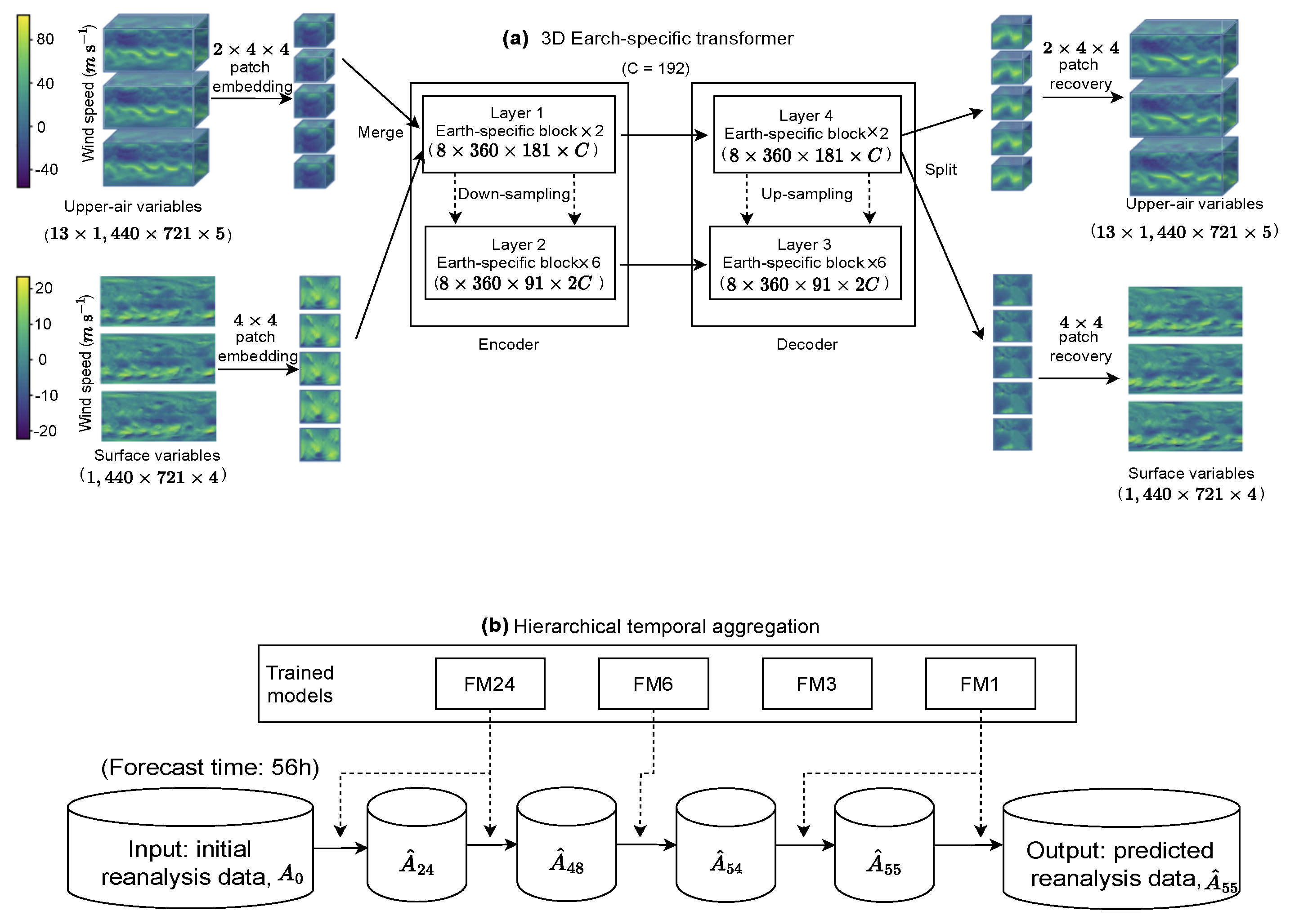
  49. Bi, K.; Xie, L.; Zhang, H.; Chen, X.; Gu, X.; Tian, Q. Accurate Medium-Range Global Weather Forecasting with 3D Neural Networks. Nature 2023, 619, 533–538. [Google Scholar] [CrossRef]
  50. Nguyen, T.; Brandstetter, J.; Kapoor, A.; Gupta, J.K.; Grover, A. ClimaX: A foundation model for weather and climate. arXiv 2023, arXiv:2301.10343. [Google Scholar]
  51. Gangopadhyay, S.; Clark, M.; Rajagopalan, B. Statistical Down-scaling using K-nearest neighbors. In Water Resources Research; Wiley Online Library: Hoboken, NJ, USA, 2005; Volume 41. [Google Scholar]
  52. Tripathi, S.; Srinivas, V.V.; Nanjundiah, R.S. Down-scaling of precipitation for climate change scenarios: A support vector machine approach. J. Hydrol. 2006, 330, 621–640. [Google Scholar] [CrossRef]
  53. Krasnopolsky, V.M.; Fox-Rabinovitz, M.S. Complex hybrid models combining deterministic and machine learning components for numerical climate modeling and weather prediction. Neural Netw. 2006, 19, 122–134. [Google Scholar] [CrossRef] [PubMed]
  54. Raje, D.; Mujumdar, P.P. A conditional random field–based Down-scaling method for assessment of climate change impact on multisite daily precipitation in the Mahanadi basin. In Water Resources Research; Wiley Online Library: Hoboken, NJ, USA, 2009; Volume 45. [Google Scholar]
  55. Zarei, M.; Najarchi, M.; Mastouri, R. Bias correction of global ensemble precipitation forecasts by Random Forest method. Earth Sci. Inform. 2021, 14, 677–689. [Google Scholar] [CrossRef]
  56. Andersson, T.R.; Hosking, J.S.; Pérez-Ortiz, M.; Paige, B.; Elliott, A.; Russell, C.; Law, S.; Jones, D.C.; Wilkinson, J.; Phillips, T.; et al. Seasonal Arctic Sea Ice Forecasting with Probabilistic Deep Learning. Nat. Commun. 2021, 12, 5124. [Google Scholar] [CrossRef] [PubMed]
  57. Wang, X.; Han, Y.; Xue, W.; Yang, G.; Zhang, G. Stable climate simulations using a realistic general circulation model with neural network parameterizations for atmospheric moist physics and radiation processes. Geosci. Model Dev. 2022, 15, 3923–3940. [Google Scholar] [CrossRef]
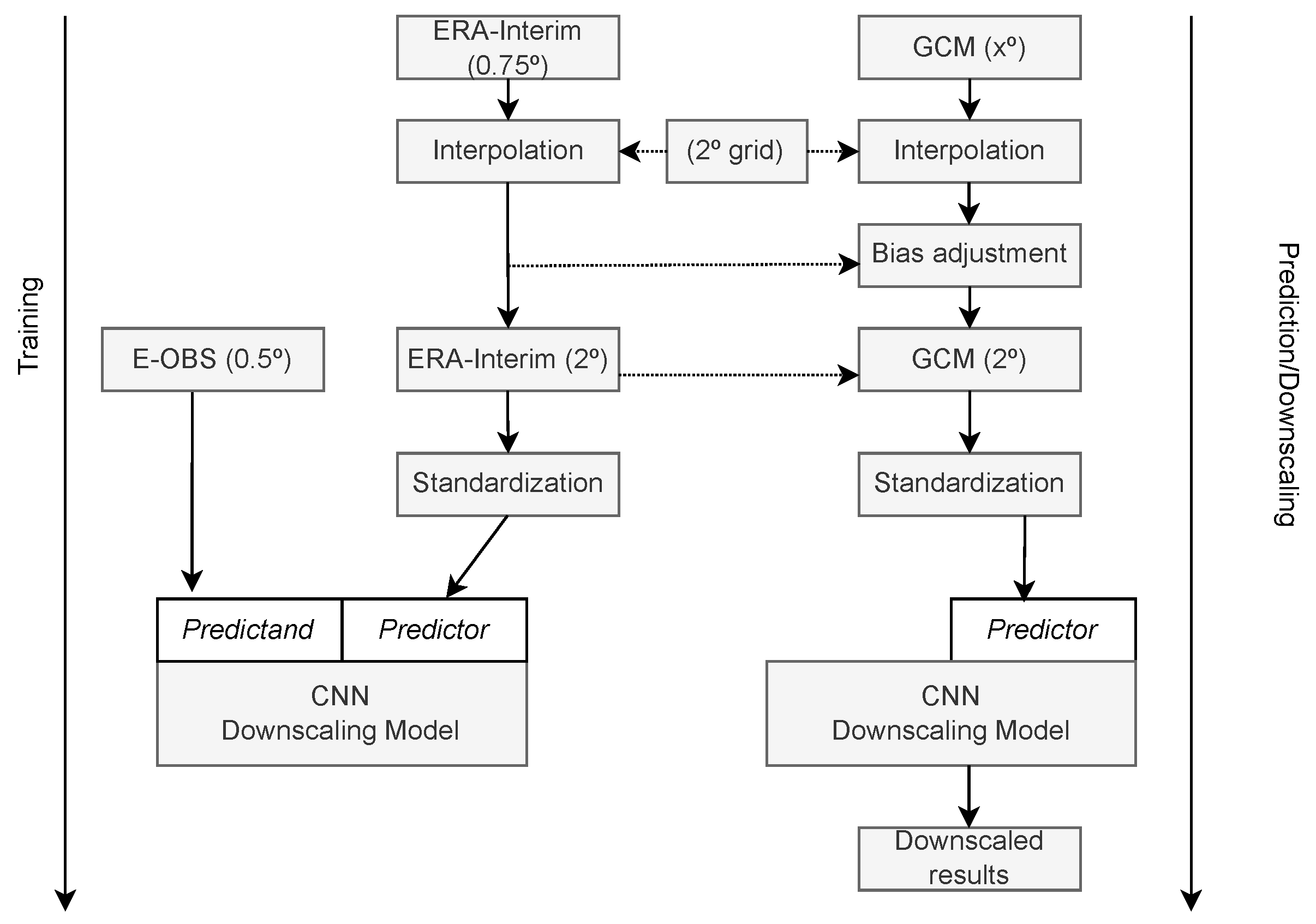
  58. Baño-Medina, J.; Manzanas, R.; Cimadevilla, E.; Fernández, J.; González-Abad, J.; Cofiño, A.S.; Gutiérrez, J.M. Down-scaling Multi-Model Climate Projection Ensembles with Deep Learning (DeepESD): Contribution to CORDEX EUR-44. Geosci. Model Dev. 2022, 15, 6747–6758. [Google Scholar] [CrossRef]
  59. Hess, P.; Lange, S.; Boers, N. Deep Learning for bias-correcting comprehensive high-resolution Earth system models. arXiv 2022, arXiv:2301.01253. [Google Scholar]
  60. Wang, F.; Tian, D. On deep learning-based bias correction and Down-scaling of multiple climate models simulations. Clim. Dyn. 2022, 59, 3451–3468. [Google Scholar] [CrossRef]
  61. Pan, B.; Anderson, G.J.; Goncalves, A.; Lucas, D.D.; Bonfils, C.J.W.; Lee, J. Improving Seasonal Forecast Using Probabilistic Deep Learning. J. Adv. Model. Earth Syst. 2022, 14, e2021MS002766. [Google Scholar] [CrossRef]
  62. Hu, Y.; Chen, L.; Wang, Z.; Li, H. SwinVRNN: A Data-Driven Ensemble Forecasting Model via Learned Distribution Perturbation. J. Adv. Model. Earth Syst. 2023, 15, e2022MS003211. [Google Scholar] [CrossRef]
  63. Chen, L.; Zhong, X.; Zhang, F.; Cheng, Y.; Xu, Y.; Qi, Y.; Li, H. FuXi: A cascade machine learning forecasting system for 15-day global weather forecast. arXiv 2023, arXiv:2306.12873. [Google Scholar]
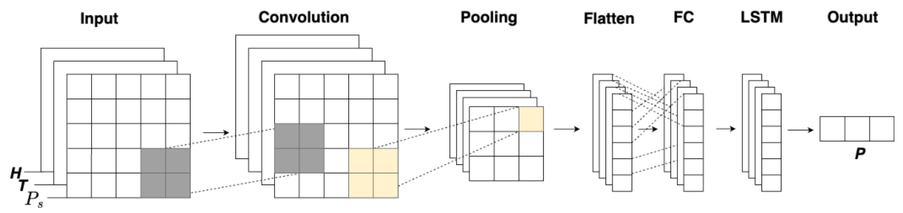
  64. Lin, H.; Gao, Z.; Xu, Y.; Wu, L.; Li, L.; Li, S.Z. Conditional local convolution for spatio-temporal meteorological forecasting. Proc. Aaai Conf. Artif. Intell. 2022, 36, 7470–7478. [Google Scholar] [CrossRef]
  65. Chen, K.; Han, T.; Gong, J.; Bai, L.; Ling, F.; Luo, J.J.; Chen, X.; Ma, L.; Zhang, T.; Su, R.; et al. FengWu: Pushing the Skillful Global Medium-range Weather Forecast beyond 10 Days Lead. arXiv 2023, arXiv:2304.02948. [Google Scholar]
  66. De Burgh-Day, C.O.; Leeuwenburg, T. Machine Learning for numerical weather and climate modelling: A review. EGUsphere 2023, 2023, 1–48. [Google Scholar]
  67. LeCun, Y.; Bottou, L.; Bengio, Y.; Haffner, P. Gradient-based learning applied to document recognition. Proc. IEEE 1998, 86, 2278–2324. [Google Scholar] [CrossRef]
  68. Krizhevsky, A.; Sutskever, I.; Hinton, G.E. ImageNet classification with deep convolutional neural networks. Adv. Neural Inf. Process. Syst. 2012, 25, 1097–1105. [Google Scholar] [CrossRef]
  69. Scherer, D.; Müller, A.; Behnke, S. Evaluation of pooling operations in convolutional architectures for object recognition. In Proceedings of the International Conference on Artificial Neural Networks 2010, Thessaloniki, Greece, 15–18 September 2010; pp. 92–101. [Google Scholar]
  70. LeCun, Y.; Bengio, Y.; Hinton, G. Deep learning. Nature 2015, 521, 436–444. [Google Scholar] [CrossRef] [PubMed]
  71. Liu, Y.; Racah, E.; Correa, J.; Khosrowshahi, A.; Lavers, D.; Kunkel, K.; Wehner, M.; Collins, W. Application of deep convolutional neural networks for detecting extreme weather in climate datasets. arXiv 2016, arXiv:1605.01156. [Google Scholar]
  72. Goodfellow, I.; Warde-Farley, D.; Mirza, M.; Courville, A.; Bengio, Y. Maxout networks. In Proceedings of the International Conference on Machine Learning, Atlanta, GA, USA, 16–21 June 2013; pp. 1319–1327. [Google Scholar]
  73. Marion, M.; Roger, T. Navier-Stokes equations: Theory and approximation. Handb. Numer. Anal. 1998, 6, 503–689. [Google Scholar]
  74. Iacono, M.J.; Mlawer, E.J.; Clough, S.A.; Morcrette, J.-J. Impact of an improved longwave radiation model, RRTM, on the energy budget and thermodynamic properties of the NCAR community climate model, CCM3. J. Geophys. Res. Atmos. 2000, 105, 14873–14890. [Google Scholar] [CrossRef]
  75. Guo, Y.; Shao, C.; Su, A. Comparative Evaluation of Rainfall Forecasts during the Summer of 2020 over Central East China. Atmosphere 2023, 14, 992. [Google Scholar] [CrossRef]
  76. Guo, Y.; Shao, C.; Su, A. Investigation of Land–Atmosphere Coupling during the Extreme Rainstorm of 20 July 2021 over Central East China. Atmosphere 2023, 14, 1474. [Google Scholar] [CrossRef]
  77. Bauer, P.; Thorpe, A.; Brunet, G. The Quiet Revolution of Numerical Weather Prediction. Nature 2015, 525, 47–55. [Google Scholar] [CrossRef] [PubMed]
  78. Vaswani, A.; Shazeer, N.; Parmar, N.; Uszkoreit, J.; Jones, L.; Gomez, A.N.; Kaiser, Ł.; Polosukhin, I. Attention is All You Need. In Proceedings of the NeurIPS, Long Beach, CA, USA, 4–9 December 2017. [Google Scholar]
  79. Wang, H.; Zhu, Y.; Green, B.; Adam, H.; Yuille, A.; Chen, L.C. Axial-DeepLab: Stand-Alone Axial-Attention for Panoptic Segmentation. arXiv 2019, arXiv:2003.07853. [Google Scholar]
  80. Schmit, T.J.; Griffith, P.; Gunshor, M.M.; Daniels, J.M.; Goodman, S.J.; Lebair, W.J. A closer look at the ABI on the GOES-R series. Bull. Am. Meteorol. Soc. 2017, 98, 681–698. [Google Scholar] [CrossRef]
  81. Li, Z.; Kovachki, N.; Azizzadenesheli, K.; Liu, B.; Bhattacharya, K.; Stuart, A.; Anandkumar, A. Fourier Neural Operator for Parametric Partial Differential Equations. In Proceedings of the International Conference on Learning Representations (ICLR), Virtual Event. 3–7 May 2021. [Google Scholar]
  82. Guibas, J.; Mardani, M.; Li, Z.; Tao, A.; Anandkumar, A.; Catanzaro, B. Adaptive Fourier Neural Operators: Efficient token mixers for transformers. In Proceedings of the International Conference on Representation Learning, Virtual Event. 25–29 April 2022. [Google Scholar]
  83. Rasp, S.; Thuerey, N. Purely data-driven medium-range weather forecasting achieves comparable skill to physical models at similar resolution. arXiv 2020, arXiv:2008.08626. [Google Scholar]
  84. Weyn, J.A.; Durran, D.R.; Caruana, R.; Cresswell-Clay, N. Sub-seasonal forecasting with a large ensemble of deep-learning weather prediction models. arXiv 2021, arXiv:2102.05107. [Google Scholar] [CrossRef]
  85. Rasp, S.; Dueben, P.D.; Scher, S.; Weyn, J.A.; Mouatadid, S.; Thuerey, N. Weatherbench: A benchmark data set for data-driven weather forecasting. J. Adv. Model. Earth Syst. 2020, 12, e2020MS002203. [Google Scholar] [CrossRef]
  86. Liu, Z.; Lin, Y.; Cao, Y.; Hu, H.; Wei, Y.; Zhang, Z.; Lin, S.; Guo, B. Swin transformer: Hierarchical vision transformer using shifted windows. In Proceedings of the International Conference on Computer Vision, Virtual. 11–17 October 2021; IEEE: New York, NY, USA, 2021; pp. 10012–10022. [Google Scholar]
  87. Dosovitskiy, A.; Beyer, L.; Kolesnikov, A.; Weissenborn, D.; Zhai, X.; Unterthiner, T.; Dehghani, M.; Minderer, M.; Heigold, G.; Gelly, S.; et al. An image is worth 16x16 words: Transformers for image recognition at scale. arXiv 2020, arXiv:2010.11929. [Google Scholar]
  88. Váňa, F.; Düben, P.; Lang, S.; Palmer, T.; Leutbecher, M.; Salmond, D.; Carver, G. Single precision in weather forecasting models: An evaluation with the IFS. Mon. Weather Rev. 2017, 145, 495–502. [Google Scholar] [CrossRef]
  89. IPCC. Climate Change 2013: The Physical Science Basis. Contribution of Working Group I to the Fifth Assessment Report of the Intergovernmental Panel on Climate Change; Cambridge University Press: Cambridge, UK; New York, NY, USA, 2013. [Google Scholar]
  90. Flato, G.; Marotzke, J.; Abiodun, B.; Braconnot, P.; Chou, S.C.; Collins, W.; Cox, P.; Driouech, F.; Emori, S.; Eyring, V.; et al. Evaluation of Climate Models. In Climate Change 2013: The Physical Science Basis. Contribution of Working Group I to the Fifth Assessment Report of the Intergovernmental Panel on Climate Change; Cambridge University Press: Cambridge, UK; New York, NY, USA, 2013. [Google Scholar]
  91. Washington, W.M.; Parkinson, C.L. An Introduction to Three-Dimensional Climate Modeling; University Science Books: Beijing, China, 2005. [Google Scholar]
  92. Giorgi, F.; Gutowski, W.J. Regional Dynamical Down-scaling and the CORDEX Initiative. Annu. Rev. Environ. Resour. 2015, 40, 467–490. [Google Scholar] [CrossRef]
  93. Randall, D.A.; Wood, R.A.; Bony, S.; Colman, R.; Fichefet, T.; Fyfe, J.; Kattsov, V.; Pitman, A.; Shukla, J.; Srinivasan, J.; et al. Climate Models and Their Evaluation. In Climate Change 2007: The Physical Science Basis. Contribution of Working Group I to the Fourth Assessment Report of the Intergovernmental Panel on Climate Change; Cambridge University Press: Cambridge, UK; New York, NY, USA, 2007. [Google Scholar]
  94. Taylor, K.E.; Stouffer, R.J.; Meehl, G.A. An overview of CMIP5 and the experiment design. Bull. Am. Meteorol. Soc. 2012, 93, 485–498. [Google Scholar] [CrossRef]
  95. Miao, C.; Shen, Y.; Sun, J. Spatial–temporal ensemble forecasting (STEFS) of high-resolution temperature using machine learning models. J. Adv. Model. Earth Syst. 2019, 11, 2961–2973. [Google Scholar]
  96. Mukkavilli, S.; Perone, C.S.; Rangapuram, S.S.; Müller, K.R. Distribution regression forests for probabilistic spatio-temporal forecasting. In Proceedings of the International Conference on Machine Learning (ICML), Vienna, Austria, 12–18 July 2020. [Google Scholar]
  97. Walker, G.; Charlton-Perez, A.; Lee, R.; Inness, P. Challenges and progress in probabilistic forecasting of convective phenomena: The 2016 GFE/EUMETSAT/NCEP/SPC severe convective weather workshop. Bull. Am. Meteorol. Soc. 2016, 97, 1829–1835. [Google Scholar]
  98. Kingma, D.P.; Welling, M. Auto-encoding variational bayes. arXiv 2013, arXiv:1312.6114. [Google Scholar]
  99. Krasting, J.P.; John, J.G.; Blanton, C.; McHugh, C.; Nikonov, S.; Radhakrishnan, A.; Zhao, M. NOAA-GFDL GFDL-ESM4 model output prepared for CMIP6 CMIP. Earth Syst. Grid Fed. 2018, 10. [Google Scholar] [CrossRef]
  100. Zhu, J.-Y.; Park, T.; Isola, P.; Efros, A.A. Unpaired image-to-image translation using cycle-consistent adversarial networks. In Proceedings of the IEEE International Conference on Computer Vision, Venice, Italy, 22–29 October 2017; pp. 2223–2232. [Google Scholar]
  101. Brands, S.; Herrera, S.; Fernández, J.; Gutiérrez, J.M. How well do CMIP5 Earth System Models simulate present climate conditions in Europe and Africa? Clim. Dynam. 2013, 41, 803–817. [Google Scholar] [CrossRef]
  102. Vautard, R.; Kadygrov, N.; Iles, C. Evaluation of the large EURO-CORDEX regional climate model ensemble. J. Geophys. Res.-Atmos. 2021, 126, e2019JD032344. [Google Scholar] [CrossRef]
  103. Boé, J.; Somot, S.; Corre, L.; Nabat, P. Large discrepancies in summer climate change over Europe as projected by global and regional climate models: Causes and consequences. Clim. Dynam. 2020, 54, 2981–3002. [Google Scholar] [CrossRef]
  104. Baño-Medina, J.; Manzanas, R.; Gutiérrez, J.M. Configuration and intercomparison of deep learning neural models for statistical Down-scaling. Geosci. Model Dev. 2020, 13, 2109–2124. [Google Scholar] [CrossRef]
  105. Lecun, Y.; Bengio, Y. Convolutional Networks for Images, Speech, and Time-Series. Handb. Brain Theory Neural Netw. 1995, 336, 1995. [Google Scholar]
  106. Dee, D.P.; Uppala, S.M.; Simmons, A.J.; Berrisford, P.; Poli, P.; Kobayashi, S.; Andrae, U.; Balmaseda, M.A.; Balsamo, G.; Bauer, D.P.; et al. The ERA-Interim reanalysis: Configuration and performance of the data assimilation system. Q. J. Roy Meteor. Soc. 2011, 137, 553–597. [Google Scholar] [CrossRef]
  107. Cornes, R.C.; van der Schrier, G.; van den Besselaar, E.J.M.; Jones, P.D. An Ensemble Version of the E-OBS Temperature and Precipitation Data Sets. J. Geophys. Res.-Atmos. 2018, 123, 9391–9409. [Google Scholar] [CrossRef]
  108. Baño-Medina, J.; Manzanas, R.; Gutiérrez, J.M. On the suitability of deep convolutional neural networks for continentalwide Down-scaling of climate change projections. Clim. Dynam. 2021, 57, 1–11. [Google Scholar] [CrossRef]
  109. Maraun, D.; Widmann, M.; Gutiérrez, J.M.; Kotlarski, S.; Chandler, R.E.; Hertig, E.; Wibig, J.; Huth, R.; Wilcke, R.A. VALUE: A framework to validate Down-scaling approaches for climate change studies. Earths Future 2015, 3, 1–14. [Google Scholar] [CrossRef]
  110. Vrac, M.; Ayar, P. Influence of Bias Correcting Predictors on Statistical Down-scaling Models. J. Appl. Meteorol. Clim. 2016, 56, 5–26. [Google Scholar] [CrossRef]
  111. Williams, P.M. Modelling Seasonality and Trends in Daily Rainfall Data. In Advances in Neural Information Processing Systems 10, Proceedings of the Neural Information Processing Systems (NIPS): Denver, Colorado, USA, 1997; MIT Press: Cambridge, MA, USA, 1998; pp. 985–991. ISBN 0-262-10076-2. [Google Scholar]
  112. Cannon, A.J. Probabilistic Multisite Precipitation Down-scaling by an Expanded Bernoulli–Gamma Density Network. J. Hydrometeorol. 2008, 9, 1284–1300. [Google Scholar] [CrossRef]
  113. Schoof, J.T. and Pryor, S.C. Down-scaling temperature and precipitation: A comparison of regression-based methods and artificial neural networks. Int. J. Climatol. 2001, 21, 773–790. [Google Scholar] [CrossRef]
  114. Maraun, D.; Widmann, M. Statistical Down-Scaling and Bias Correction for Climate Research; Cambridge University Press: Cambridge, UK, 2018; ISBN 9781107588783. [Google Scholar]
  115. Vrac, M.; Stein, M.; Hayhoe, K.; Liang, X.-Z. A general method for validating statistical Down-scaling methods under future climate change. Geophys. Res. Lett. 2007, 34, L18701. [Google Scholar] [CrossRef]
  116. San-Martín, D.; Manzanas, R.; Brands, S.; Herrera, S.; Gutiérrez, J.M. Reassessing Model Uncertainty for Regional Projections of Precipitation with an Ensemble of Statistical Down-scaling Methods. J. Clim. 2017, 30, 203–223. [Google Scholar] [CrossRef]
  117. Quesada-Chacón, D.; Barfus, K.; Bernhofer, C. Climate change projections and extremes for Costa Rica using tailored predictors from CORDEX model output through statistical Down-scaling with artificial neural networks. Int. J. Climatol. 2021, 41, 211–232. [Google Scholar] [CrossRef]
Figure 1. Applications: of machine-learning on climate prediction milestone [41,42,43,44,45,46,47,48,49,50,51,52,53,54,55,56,57,58,59,60,61].
Applsci 13 12019 g001
Figure 2. MetNet Structure.
Applsci 13 12019 g002
Figure 3. (a) The multi-layer transformer architecture; (b) two-step fine-tuning; (c) backbone model; (d) forecast model in free-running autoregressive inference mode.
Applsci 13 12019 g003
Figure 4. (a) The encoder component of the GraphCast architecture maps the input local regions (green boxes) to the nodes of the multigrid graph. (b) The processor component uses learned message passing to update each multigrid node. (c) The decoder component maps the processed multigrid features (purple nodes) to the grid representation. (d) A multi-scale grid set.
Applsci 13 12019 g004
Figure 5. Network training and inference strategies. (a) 3DEST architecture. (b) Hierarchical temporal aggregation. We use FM1, FM3, FM6 and FM24 to indicate the forecast models with lead times being 1 h, 3 h, 6 h or 24 h, respectively.
Applsci 13 12019 g005
Figure 6. Conditonal Generative Forecasting (CGF) model.
Applsci 13 12019 g006
Figure 7. CycleGAN flow chart.
Applsci 13 12019 g007
Figure 8. DeepESD structure.
Applsci 13 12019 g008
Table 1. Applications of Short term and medium-long term weather/climate forecasting in daily life.
Time ScaleDomainsApplications
Short TermAgricultureThe timing for sowing and harvesting;
Irrigation and fertilization plans [5].
EnergyPredicts output for wind and solar energy [6].
TransportationRoad traffic safety; Rail transport;
Aviation and maritime industries [7].
ConstructionProject plans and timelines; Safe operations [8].
Retail and SalesAdjusts inventory based on weather forecasts [9].
Tourism and
Entertainment
Operations of outdoor activities
and tourist attractions [10]
Environment and
Disaster Management
Early warnings for floods, fires,
and other natural disasters [11].
Medium—Long TermAgricultureLong-term land management and planning [12].
InsurancePreparations for future increases in
types of disasters, such as floods and droughts [13].
Real EstateAssessment of future sea-level rise or other
climate-related factors [14].
Urban PlanningWater resource management [15].
TourismLong-term investments and planning,
such as deciding which regions may become
popular tourist destinations in the future [16].
Public HealthLong-term climate changes may impact the
spread of diseases [17].
Table 2. Classification of models.
Time ScaleSpational ScaleTypeModelTechnologyNameEvent
Short-term weather predictionGlobalMLSpecial DNN ModelsAFNOFourCastNet [47]Extreme Events
3D Neural NetworkPanGu [49]
Vision TransformersClimaX [50]Temperature & Extreme
Event
SwinTransformerSwinVRNN [62]Temperature & Precipitation
U-TransformerFuXi [63]
Single DNNs ModelGNNCLCRN [64]Temperature
GraphCast [48]
TransformerFengWu [65]Extreme Events
Regional CapsNet [45]
CNNPrecipitation Convolution
prediction [43]
Precipitation
ANNPrecipitation Neural
Network prediction [41]
LSTMStacked-LSTM-Model [44]Temperature
Hybrid DNNs ModelLSTM + CNNConsvLSTM [42]Precipitation
MetNet [46]
Medium-to-long-term climate predictionGlobal Single DNN modelsProbalistic deep learningConditional Generative
Forecasting [61]
Temperature & Precipitation
ML EnhancedCNNCNN-Bias-correction
model [60]
Temperature & Extreme
Event
GANCycle GAN [59]Precipitation
NNHybrid-GCM-Emulation [53]
ResDNNNNCAM-emulation [57]
RegionalCNNDeepESD-Down-scaling
model [58]
Temperature
Non-Deep-Learning
Model
Random forest (RF)RF-bias-correction model [55]Precipitation
Support vector
machine (SVM)
SVM-Down-scaling model [52]
K-nearest
neighbor (KNN)
KNN-Down-scaling model [51]
Conditional random
field (CRF)
CRF-Down-scaling model [54]
Table 3. Short-term weather forecast model result comparison.
ModelForecast-TimelinessZ500 RMSE (7 Days)Z500 ACC (7 Days)Training-ComplexityForecasting-Speed
MetNet [46]8 h--256 Google-TPU-accelerators (16-days-training)Fewer seconds
FourCastNet [47]7 days5950.7624 A100-GPU24-h forecast for 100 members in 7 s
GraphCast [48]9.75 days4600.82532 Cloud-TPU-V4 (21-days-training)10-days-predication within 1 min
PanGu [49]7 days5100.872192 V100-GPU (16-days-training)24-h-global-prediction in 1.4 s for each GPU
IFS [88]8.5 days4390.85--
Table 4. Medium-to-long term climate prediction model result comparison.
NameCategoriesMetricsESMThis Model
CycleGAN [59]Bias correctionMAE0.2410.068
DeepESD [58]Down-scalingEuclidean Distance to Observations in PDF0.50.03
CGF [61]PredictionACC0.310.4
NNCAM [57]EmulationSpeed130 times speed-up
Disclaimer/Publisher’s Note: The statements, opinions and data contained in all publications are solely those of the individual author(s) and contributor(s) and not of MDPI and/or the editor(s). MDPI and/or the editor(s) disclaim responsibility for any injury to people or property resulting from any ideas, methods, instructions or products referred to in the content.

