Abstract
In this work, the applicability of a Firefly Algorithm (FA) to the real problem of the minimum cost of a detailed design for steel frames is studied. To reduce the calculation time, which is a common problem of meta-heuristic algorithms when they are used to solve real design cases, and to better suit the characteristics of the algorithm, a parallel migration strategy has been implemented and tested. As it is well known that the performance of any metaheuristic algorithm depends on the chosen value of its parameters, an extensive sensitivity analysis has been carried out. This not only serves to improve performance but also provides information on how it depends on the values of these parameters. With the information obtained from this analysis, and in order to achieve the robust behavior of the algorithm, a parameter control strategy has also been implemented and tested. Finally, a study demonstrating the close dependence between one of the parameters and the number of variables considered in the examples has been carried out. As a result of this final study, a simple expression is proposed that provides the minimum necessary population based on the number of variables in the problem.
1. Introduction
In the last three decades, a notable effort has been made to propose new design methods in the fields of meta-heuristic optimization and artificial intelligence. In these fields, biologically inspired algorithms, such as swarm-based methods, have proliferated [1]. These algorithms are currently being successfully applied to optimal design problems, image processing, business management, machine learning, and other areas. After the proposal of these new methods, initially tested on complex but idealized problems, other researchers have worked on adapting them to real engineering problems. This second line of research became necessary after the discovery of “no free lunch” (NFL) theorems [2,3], which established that no algorithm is better than another to solve a specific problem. The best algorithms are those that perform well in a specific case after adjusting their approach.
In addition to these works on the proposal and development of new algorithms and their applications and adjustments to specific cases, other authors have focused on studying the differences in their performance or new strategies to improve it. Joshi and Bansal [4] propose a generalized strategy to find the most suitable value of any parameter for a meta-heuristic algorithm. Loubière et al. [5] improve an Artificial Bee Colony (ABC) optimization algorithm using a sensitivity analysis method. Younis and Yang [6] propose two tightly coupled hybrid metaheuristic schedulers. The first scheduler combines Ant Colony Optimization (ACO) and Variable Neighborhood Search (VNS), in which ACO acts as the main algorithm that calls VNS as a supporting algorithm during execution. The second scheduler merges the Genetic Algorithm (GA) with VNS in the same way. The FA, which is a swarm-based method, has been shown to be more efficient than GA and Particle Swarm Optimization (PSO) [7]. A simple analysis of FA shows that Differential Evolution (DE), Accelerated Particle Swarm Optimization (APSO), Simulated Annealing (SA), and Harmony Search (HS) are variants of FA [1]. This has increased FA’s popularity, and it has been used to solve not only theoretical problems but also real cases [8].
Moreover, FA can manage a population divided into subpopulations simply. Each population can swarm around a local optimum, allowing the set of subpopulations to yield information in the entire design space. Finally, the global optimum can be detected among all the local optima. If the attractiveness parameter is properly adjusted, the algorithm evolves, causing the visibility among subpopulations to increase as the process progresses. This facilitates exploration at the beginning and exploitation at the end of the process [9].
This strategy of dividing the total population into subpopulations also facilitates the parallelization of the process to reduce calculation times. Some previous studies suggested that parallelization seemed to be the only general strategy capable of reducing computation times in its applicability to real engineering cases. Leite and Topping [10] evaluate parallelization strategies applied to engineering problems, where design spaces can be very complex and highly constrained, with function evaluations ranging from medium to high cost. Thierauf and Cai [11] present a method for solving mixed-discrete structural optimization problems based on a two-level parallel evolution strategy. Later, Gomes and Esposito [12], Hasançebi et al. [13], and Truong et al. [14] proposed parallelization techniques applied to real steel structures that ensured precise optimal solutions with clearly reduced calculation times. The strategy of parallelizing the process has been extended not only to structures but also to other fields of engineering [15,16,17].
For all these reasons, FA seems a good algorithm candidate for solving complex, real design problems. Gandomi et al. [18] use an FA to solve classical mixed continuous/discrete structural optimization problems. Talatahari et al. [19] present an adaptive FA, which uses a feasibility-based method for handling constraints to determine the optimal design of tower-shaped structures. Talbi [20] provides comprehensive information on meta-heuristic algorithms, including FA, to solve complex optimization problems in a wide range of applications, from networking and bioinformatics to engineering design, routing, and scheduling.
An example of this type of problem is the optimal design of steel structures, where the number of variables is usually high, and the objective function and constraints are often nonlinear. Once the algorithm has been selected as a synthesis tool, it must be defined to be efficient and robust. This involves not only establishing a simple and consistent formulation for the objective function and the constraints that can guarantee its good performance [21] but also tuning the algorithm’s parameters to ensure solutions close to the global optimum [22].
This paper studies the applicability of an FA to the real problem of the minimum-cost, detailed design of steel frames. Our main objective is to achieve a robust and efficient design method. The concept of robustness is linked to stability. The concept of efficiency is linked to reducing computational cost and calculation times.
A parallelization strategy, based on dividing the total population of fireflies into subpopulations, has been used to reduce computation time. The random migration of some fireflies among subpopulations allows them to exchange information. This parallelization–migration strategy has already been successfully tested in other problems, such as in the design of concrete sections subjected to biaxial bending [23].
A sensitivity analysis has been performed, and appropriate algorithm parameter values have been established. A new parameter control strategy has been implemented and tested with the information obtained in the sensitivity analysis to achieve an algorithm that behaves robustly. This new strategy takes advantage of subpopulations to explore different landscapes and thus allows us to obtain the different best values of the same parameter in each of the subpopulations.
Finally, a study demonstrating the close dependence between one of the parameters, which greatly affects the computational cost of the proposed numerical procedure, and the number of variables considered in the examples, has been carried out. As a result of this final study, a simple expression is proposed that is easy to memorize and provides the minimum necessary population based on the number of variables in the problem. This expression allows the designer to considerably reduce calculation time by testing different values of this minimum necessary population to achieve adequate performance.
Two steel frame design problems demonstrate the effectiveness and robustness of the proposed design method.
2. Optimum Design Problem
2.1. General Optimal Design Problem
Generally speaking, an optimal design problem, or optimization problem, is one that seeks the values of design variables that: (i) provide the minimum (or maximum) value for an objective function and (ii) provide valid (or not violated) values for a set of design constraints.
The design variables of a structure can be properties of the cross-section of the elements (areas, thicknesses, moments of inertia, etc.), geometric parameters, topological parameters, and material properties. The weight of the structure is the most common objective function. Other objective functions, such as cost, reliability, stiffness, etc., are used in other applications. Constraints are the conditions the design must meet to be valid according to design codes or standards.
The problem of calculating the minimum cost design of a steel frame can be generally stated as follows:
to find the design variable vector
to minimize the objective function (total cost of the structure)
subject to the constraints
where X is the nv-dimensional design variable vector, f(X) is the objective function, gc(X) is inequality constraint c, nc is the total number of constraints, XvL is the lower bound for variable v, Xv is variable v, XvU is the upper bound for variable v, and nv is the number of design variables.
X (X1, X2, …, Xnv)
f(X)
gc(X) ≥ 0; c = 1, 2, …, nc
XvL ≤ Xv ≤ XvU; v = 1, 2, …, nv
The most complex optimization problems, including the two examples presented in this work, are those in which the following applies:
- There are a large number of variables (1) and large scales (XvU − XvL) (4), creating an extensive design space.
- The variables are discrete or a mixture of continuous/discrete variables.
- The objective function (2) is non-linear, and the constraints (3) are many and non-linear. Cases in which derivatives of the objective function and the constraints appear at some point in the design space with values close to zero (functions insensitive to variables) or very high (jumps) are especially difficult to solve.
One reason meta-heuristic algorithms have become popular is because they can successfully address these problems. The disadvantage they present is their high computational cost. Therefore, it is essential to improve the algorithm’s performance by tuning its parameters [1,20].
2.2. The Firefly Algorithm
Meta-heuristic methods can be used to solve this problem. Among these methods is the FA, which belongs to the group of so-called nature-inspired algorithms. The FA is a swarm-based method whose search strategy depends on two sequential phases: exploration and exploitation. The first focuses on finding the global optimum throughout the design space. The second focuses on selecting the best design found up to that point among several options. During the process, the algorithm parameters change their values to encourage one or the other of these two phases [1].
The FA reproduces the social behavior of fireflies in a simple and idealized way. Fireflies communicate with each other, search for prey, and find a mate using different patterns of bioluminescent flashes [1]. The characteristics of these flashes have been idealized to develop this algorithm. Similar to real fireflies flying through 3D space and changing their spatial coordinates, the fireflies fly through nv-dimensional space, where the coordinates are now the variables of the design problem (1). The best design corresponds to a firefly i that flashes more than the others because it is in a position that minimizes a function. This is called the fitness function. The fitness function takes into account the objective function (2) and inequality constraints (3) that are violated (gc(X) < 0). During the process, the algorithm ensures that the variables (1) are within the limits (4) that define the design space.
The FA is guided by two basic rules:
- A firefly’s brightness is inversely proportional to the fitness function, so the firefly in the population with the lowest fitness function value (lowest cost and fewest constraint violations) shines brighter than the rest of the population. Fireflies are ordered by their brightness from the brightest to the dimmest in the population.
- Fireflies have no gender, so any one can be attracted to another in the population. The attraction between two fireflies, i and j, in the population decreases with the distance between them. The dimmer firefly i moves toward the brighter one j. The attraction between them is defined as
The position of a firefly i attracted to another, brighter firefly j in the population is obtained with the following expression:
where is the nv-dimensional vector of variables (or coordinates) of the i-th firefly, is the nv-dimensional vector of variables of the j-th firefly, and rij is the Cartesian distance in the nv-dimensional space obtained as follows:
2.3. Variables
The total population of fireflies (nt) is established by means of an array, which is a set of data organized in rows, columns, and planes. The data stored in the array are the values of the variables (1). In each plane of the array, we have a matrix representing a subpopulation of fireflies, so we will have as many planes (np) as there are subpopulations. Each matrix has as many rows as there are fireflies in each subpopulation (n) and as many columns as variables considered in the problem (nv). Thus, each firefly is assigned a set of variable values representing a particular design X (1). At the beginning of the process, the values of the variables stored in the array are randomly determined within the bounds (4) of the design space.
In each particular design X, there are variables assigned to elements (beams or columns of the structure) and variables assigned to the semi-rigid connections (end-plates and bolts) between the elements. The variables assigned to the elements are the areas of the section. The variables assigned to the semi-rigid connections are the thickness of the end-plates and the diameter of the bolts used. Therefore, a particular design X includes as many area values as there are steel shapes for the elements and as many values of end-plate thicknesses and bolt diameters as there are semi-rigid connections.
To find the discrete values (DV) of the variables, either those associated with commercial steel shapes (IPE or HEB), the thicknesses of commercial steel end-plates, or the diameters of commercial steel bolts, a randomized rounding approach has been established. This approach compares the continuous value (CV) of a variable obtained during the procedure with a value obtained at random (RV) between two limits: (i) the commercial value immediately below the CV of the variable (lower commercial value or LCV) and (ii) the commercial value immediately above the CV of the variable (upper commercial value or UCV). If the CV is less than the RV, the DV adopted for the variable is the LCV. If the CV is greater than the RV, the DV adopted for the variable is the UCV (Figure 1).

Figure 1.
Rounding approach for a continuous variable: DV = UCV.
This rounding procedure favors adopting the value of the closest limit (LCV or UCV) for the DV of the variable. However, if the CV of the variable is halfway between both limits (close to the mean), neither of them is favored since the probability of adopting either is similar (Figure 2).
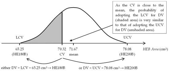
Figure 2.
Rounding approach for a continuous variable: either DV = LCV or DV = UCV.
This procedure of rounding continuous variables to discrete values avoids creating a bias in the process as much as possible so that during the exploration phase, there is a similar probability of choosing the LCV or the UCV, and, during the exploitation phase, of choosing the value of the LCV or the UCV closest to the CV of the variables.
As the variables used for elements are areas, and the variables for semi-rigid connections are plate thicknesses and bolt diameters, the orders of magnitude of these variables may be somewhat different. For example, using International System units, it is possible to have an area of 0.001643 m2 (IPE140), an end-plate with a thickness of 0.018 m, and bolts with a diameter of 0.020 m. This can reduce the effectiveness of the algorithm. It is only necessary to divide the value of the variables, called design variables X, by their upper limits to eliminate this problem. These new variables P are called optimization variables or coordinates because these coordinates are used by the algorithm to obtain new coordinates for the fireflies. For example, if an area of 0.0156 m2 (IPE600), an end-plate with a thickness of 0.040 m, and a bolt with a diameter of 0.036 m are chosen as upper limits, the previous design variables (0.001643, 0.018, and 0.020) correspond to the optimization variables 0.1053, 0.4500, and 0.5556, respectively.
The design variables X can be obtained at any time from the optimization variables P by multiplying their values by those of their upper limits, for example, after obtaining new firefly coordinates. But since the values of the coordinates P are continuous, the values of the design variables X will also be continuous (CV). Therefore, they must be rounded randomly, as explained above, to obtain commercial values (DV). Only then will realistic designs X and realistic values of the objective function f(X) and constraints gc(X) be obtained.
2.4. Fitness Function
A detailed description of the fitness function can be found in the previous work by Sánchez-Olivares and Tomás [21]. To facilitate reading, a brief description is included here. The fitness function is defined as
where Xi = (Xi1, Xi2, …, Xinv) is the nv-dimensional design variable vector obtained by the algorithm for firefly i in the current iteration, f(Xi) is the total cost of design Xi, is the nv-dimensional design variable vector randomly obtained for firefly i in the first iteration, f() is the total cost of design , and nvc is the number of violated constraints (gc(Xi) < 0) for firefly i in the current iteration.
2.5. Constraints
The following expressions of the constraints have been established following the requirements of Eurocode 3 [24]. A detailed description of the constraints can be found in the previous work by Sánchez-Olivares and Tomás [21]. A brief description is included here.
2.5.1. Story Lateral Sway Constraints
The normalized form of a frame story lateral sway constraint is
where Dm is the displacement, as an absolute value, of the degree of freedom m and is the maximum displacement allowed for the degree of freedom m.
2.5.2. Beam Deflection Constraints
The normalized form of a frame beam bending deflection constraint is
where vl is the flexural deflection, as an absolute value, of beam l, and is the maximum deflection allowed for beam l.
2.5.3. Slenderness Constraints
The normalized form of a frame member (beam or column) slenderness constraint is
where Kl is the effective column-length factor of member l; Ll is the length of member l; il is the radius of gyration around the relevant axis of member l; E is Young’s modulus of steel; fy is the specified yield strength of steel; and is the maximum in-plane non-dimensional slenderness allowed for member l.
2.5.4. Buckling Constraints
The normalized form of a frame member buckling constraint is as follows:
- for Class 1 and Class 2 cross-sections
- for Class 3 cross-sections
- for Class 4 cross-sections
2.5.5. Strength Constraints
The normalized form of a frame member strength constraint is as follows:
- for Class 1 and Class 2 cross-sections
- for Class 3 cross-sections
- for Class 4 cross-sections
2.5.6. Semi-Rigid Connection Strength Constraints
The normalized form of a frame semi-rigid strength constraint is
where Mlk is the factored bending moment of member l and end k, and Mlk,Rd is the design moment resistance of the semi-rigid connection of member l and end k.
2.5.7. Semi-Rigid Connection Assembly Constraints
The normalized form of a frame semi-rigid connection assembly constraint is
where is the bolt diameter adopted for the semi-rigid connection of member l and end k, and is the maximum bolt diameter allowed for the semi-rigid connection of member l and end k.
3. Optimization Methodology
3.1. Parallel Firefly Algorithm with Migration (PFAM)
The PFAM reproduces the complex social behavior of real fireflies in a simplified way. This simple or idealized behavior is guided by four basic rules:
- The population is divided into subpopulations that extend the search throughout the design space. This division into subpopulations favors finding local optima in the exploration phase. From among all the local optima found, the best local optimum is selected at the end of the process in the exploitation phase. This becomes a candidate for the global optimum, as previously mentioned [9]. Dividing the population into subpopulations also makes it easier to parallelize the algorithm [23]. A MATLAB® code has been defined to implement this parallel strategy using the MATLAB® parfor command.
- A firefly’s brightness is inversely proportional to the fitness function, so the firefly in the subpopulation with the lowest fitness function value (lowest cost and fewest constraint violations) shines brighter than the rest of the subpopulation. Fireflies are ordered by their brightness from the brightest to the dimmest in each subpopulation.
- Fireflies have no gender, so any one can be attracted to another in a subpopulation. The position of a firefly i in a subpopulation, which is attracted to another, brighter firefly j in the same subpopulation, is obtained using the following expression
And Cq is a simplified form of a sinusoidal chaotic variable at the q-th iteration in which 0 ˂ Cq ˂ 1, which is defined as follows [27]:
- iv.
- Some fireflies from the subpopulation containing the brightest firefly of all the subpopulations (origin subpopulation) are randomly selected and sent to other randomly selected subpopulations. This process of migration allows the fireflies to share information. As the origin subpopulation is the one yielding information, there is a risk that the search for the other subpopulations might be conditioned to include the local optimum. This can result in a biased search, with the search for local optima favored over a global optimum. To reduce this potential bias, a simple strategy consisting of perturbing the best design in the origin population and in each subpopulation has been included in the algorithm [23]. Therefore, if these best designs in each subpopulation are local optima, the perturbation eliminates this status, at least during the next iteration. The perturbation of the brightest firefly (i = 1) in a subpopulation is defined using the following expression:
3.2. Parameter Tuning in PFAM
Selecting the parameters is vital to achieving good results from the algorithm. However, this is complicated by the nonlinear interdependence among the parameters and because their value also depends on the fitness landscape. Furthermore, a parameter setting that provides good results in some cases may be inappropriate in others. When the parameter is inappropriate, the problem of robustness appears. This adjustment should provide at least acceptable results for a wide range of problems [28].
Parameter tuning can be considered from two different perspectives [22]:
- configuring an algorithm by choosing parameter values that optimize its performance; or
- analyzing an algorithm by studying how its performance depends on the values of its parameters.
The first perspective involves finding the optimal configuration of the algorithm. Extensive knowledge about the information the algorithm can find while traversing the design space is not essential. The second perspective involves finding more information that reveals the robustness of the algorithm, the distribution of the quality of the solutions, the sensitivity, etc. Both perspectives have been considered in this work, but the second one is more closely related to the concept of robustness. According to Eiben and Smit [22], many definitions of robustness can be obtained by extending the two previous perspectives with the following:
- iii.
- analyzing an algorithm to see how its performance varies when different problems are considered; and
- iv.
- analyzing an algorithm to see how its performance changes when it is executed several times independently.
Therefore, different problems must be analyzed to see how different executions of the algorithm applied to each of these problems provide information about its stability. These issues are addressed in this paper, but before establishing a study strategy to clarify them, some relevant information on FA parameters should be considered.
Some studies deal with the problem of establishing FA parameter values [9,18,27]. In general, the FA is very efficient, but an oscillatory behavior problem can appear [7,9]. This problem is avoided by reducing the randomization parameter as the search process progresses. The work of the authors of reference [18] indicates that, in most cases, a value of is adequate.
Another FA parameter that greatly affects its behavior is the absorption coefficient γ [1]. This parameter influences attractiveness. Its value is more or less influential depending on whether we are in the exploration phase or the exploitation phase. In the exploitation phase, it determines convergence speed since, in expression (23), the third term has less weight than the second. When γ is small, the attractiveness is constant, so all the fireflies can be seen in a transparent medium. However, when γ is large, the attractiveness decreases, and the fireflies fly in a foggy space, making it difficult for them to see each other. When this happens, the fireflies move almost randomly, which entails a random search. As a result, the behavior of the FA is halfway between these two extreme situations. Some authors have determined that, in practice, this parameter takes values from the interval [0.01, 10] [8,12].
The implemented MATLAB® code allows the randomization parameter α [7,9] and the absorption coefficient γ to be reduced as the process progresses [25]. This strategy makes it possible to gradually move from the exploration phase to the exploitation phase. If kmax is the maximum number of iterations and k is the current iteration, the variable t = k / kmax can define the function (Figure 3).
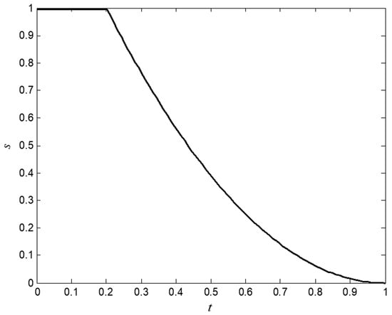
Figure 3.
Function s(t) with tc = 0.2.
And the new randomization parameter α(t) and absorption coefficient γ(t) are
The simplest strategy is to set [7], where L is the typical length of the design variables, and relate the randomization parameter α to the actual scale of each design variable [18]. For this reason, and because the optimization variables are normalized in this work, the values of α0 and γ0 throughout the unit can be adopted in expressions (28) and (29).
These basic operations were implemented in MATLAB® and are summarized in the Appendix A.
According to expression (5), parameters β0 and m also affect attractiveness, with β0 being that with the most direct and simple effect [1]. Parameter m only has a minor influence. A value of m ⸦ [1,3] can be taken [1]. A constant value of β0 = 1 can be adopted, since this value has been proven suitable in most of the design examples studied in the literature [1,18,29].

Table 1.
FA and PFAM parameters to be tuned.
This study strategy is based on the concept of robustness and how this concept is associated with different design problems, parametric values, and independent executions [22]. Design problems of the same structural typology widely used in construction have been considered. In each of these problems, the behavior of the PFAM with different parametric values has been studied, and several independent executions have been performed. A value of β0 = 1 has been adopted following studies by previously mentioned authors, and changes have been considered in the rest of the parameters included in Table 1.
3.3. Parameter Control in PFAM
An extensive classification and review of tuning and parameter control methods can be found in the work of Eiben and Smit [22]. According to these authors, there are two possible ways to proceed with parameter tuning: (i) exploiting knowledge or finding the set of parameters that provides the best performance, and (ii) exploring parameter space, which involves searching for the most information about the robustness of the process. Tuning methods generally balance exploitation and exploration and establish different categories of robustness. In the classification by Eiben and Smit [22], there are four main approaches: one based on only finding the best set of parameters (meta-EA), another based only on searching for information (sampling), and two that are a mixture of exploitation and exploration (screening and model-based).
The screening approach provides information on the influence of a model’s parametric values through an efficient exploration of multidimensional space [5]. One screening method is Morris’ Elementary Effect (EE) [30]. This method can detect the parameters that influence the model as well as their interactions. A sensitivity analysis allows the influence of an input II parameter πz on a function F to be detected and quantified. The elementary effect (EEz) of πz on F can be obtained using the expression (30)
where ∆ is an offset and D is the number of parameters.
A variant of this screening method was proposed by Joshi and Bansal [4]. The method proposed by these authors is a parameter control method applied to a metaheuristic algorithm (Gravitational Search Algorithm, GSA). The same authors commented that the screening method included in GSA (Parameter Tuning in Gravitational Search Algorithm, PTGSA) could be applied to other metaheuristic algorithms apart from GSA. In their work, the authors checked the robustness of the PTGSA method by applying it to 15 unconstrained continuous test functions of the CEC 2015 test suite [31]. Additionally, they compared the PTGSA method with other metaheuristic algorithms to evaluate its performance and robustness.
A parameter control method adapted to the proposed algorithm PFAM (Parameter Control in Parallel Firefly Algorithm with Migration, PCPFAM) was applied to solve the design problem of steel structures (expressions 5 to 19). The design problems previously used to verify the robustness of PFAM were considered to verify the efficiency of PCPFAM.
In this work, the elementary effects are calculated from the differences in the value of the fitness function F when a k-th iteration is performed in the process, and the value of the z-th parameter πz is modified, according to the expression (31)
where
Therefore, according to (31), the elementary effect for firefly i in the k-th iteration, when the value of the z-th parameter πz is modified, can be obtained using the following expression
Or
In addition, comparing expressions (31) and (36), it is evident that the following expression holds:
Figure 4 shows a hypothetical evolution of an Fi-landscape between two consecutive iterations, k − 1 and k, and between two consecutive m − 1 and m iterations.
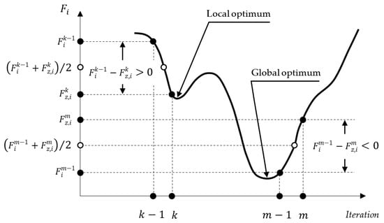
Figure 4.
Evolution of Fi—landscape between consecutive iterations.
In other words, the elementary effect gives us a measure of the change in Fi due to a change in the position of firefly i under the influence of the change in the value of parameter πz at the k-th iteration.
If the following expressions hold
Then
Being that
So the is larger when changes in the position of firefly i occur near a global optimum. Thus, the larger the change in Fi and the closer firefly i is to a global optimum, the larger the value of .
As rarely occurs, weights calculated from the are adopted here as below:
Once the values of for the n fireflies of a subpopulation have been calculated at the k-th iteration, they are stored in an array that has as many dimensions as parameters to tune, plus an additional dimension for the n fireflies in the subpopulation. For example, if there are n fireflies and two parameters to tune with dimensions D1 and D2
The values of the weights
are stored at the k-th iteration in an array of D1 rows, D2 columns, and n planes, as follows:
It is possible to obtain a measure of the impact or influence that the value of parameter πz has on the entire subpopulation when the process advances one iteration k. To achieve this, the mean of is calculated using the following expression:
which has been adopted.
In this work, the mean value is stored in an array assigned to each subpopulation. This array has as many dimensions as there are parameters to tune. For example, if there are two parameters to tune with dimensions D1 and D2, the values of the means
are stored in an array of D1 rows and D2 columns as follows:
Once array has been updated, the algorithm selects the maximum value stored in it. The values of parameters and to be used in the next iteration k+1 correspond to the -row and -column of where the maximum value
is stored as follows:
With this procedure, it is possible to improve the performance of the algorithm by selecting the and parameters in and in , respectively, that maximize the changes in the given landscape Fi, especially those produced in coordinates close to a global optimum.
There are several possibilities for how the algorithm selects the specific value of a parameter from among the D values included in . A simple way to proceed is to directly assign D values for that fall within a range so that there is a correspondence between each value in and each mean in . However, the question arises as to how many D-values to consider in . If D is a large value, there will be many values not only in but also in , which makes it more expensive to select and . Another possibility is to obtain an estimate of from the values stored in . In this work, this second possibility was chosen, considering three unique values
with
regardless of the number of parameters to consider. If, for example, two parameters are considered
then is a matrix with three rows and three columns with the following configuration:
The estimation of was performed in this work using the Lagrange polynomials . With three unique values for according to expression (56), the three corresponding Lagrange’s polynomials are as follows:
from which function can be defined as follows:
Function is represented in Figure 5. This function allows the maximum estimated value and parameter to be obtained.
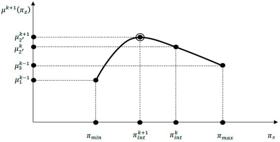
Figure 5.
Function , estimated maximun value , and obtained parameter .
This parameter control procedure was integrated into the PFAM in MATLAB®, obtaining the PCPFAM algorithm, whose basic operations are summarized in the Appendix A.
The performance of the PCPFAM algorithm was verified using two design examples, which have been extensively studied by several authors and are presented below.
4. Examples
4.1. Three-Bay Two-Story Framework
The three-bay two-story structure shown in Figure 6, Figure 7 and Figure 8 has been previously studied by Cabrero and Bayo [32], Ali et al. [33], and Sánchez-Olivares and Tomás [21]. Figure 6 shows the geometry of the structure and the loads considered. The load factors that have been considered are γG = 1.3 for self-weight loads (qsw) and γQ = 1.5 for imposed (qil) and wind (qw) loads.
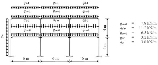
Figure 6.
Geometry and loads for the three-bay two-story framework.
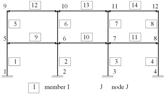
Figure 7.
Node and member numbers for the three-bay two-story framework.
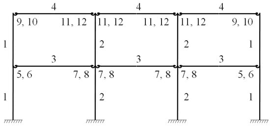
Figure 8.
Number of variables for the three-bay two-story framework.
Figure 7 shows the numbering used for the nodes and members. The expressions from 6 to 19 have been considered following the requirements of Eurocode 3 [24]. The columns and beams have HEB and IPE steel shapes, respectively.
The material considered for the steel shapes in members and steel end-plates in semi-rigid connections was steel S275 with Young’s modulus E = 210 GPa, fy = 275 MPa yield strength, and a resistance factor of γm = 1.0. The ultimate tensile strength and the resistance factor considered for bolts in the semi-rigid connections were fub = 800 MPa and γm = 1.25, respectively. The material cost of the steel considered was C = 1.6 EUR/kg. The cost of the rigid connections in the frame was calculated assuming a fixity factor of 0.964 [21]. To model the behavior of the extended end-plates with stiffened column flange semi-rigid connections (EEP1) and extended end-plates without stiffened column flange semi-rigid connections (EEP2), the Component Method was used.
Figure 8 shows the numbering used for the design variables. The design variables are included in Table 2.
Table 2.
Design variables for the three-bay two-story framework.
The PFAM algorithm was run 100 times using different random seeds to guarantee that the best-generated solution would be considered the optimal design solution. Ten subpopulations were considered in all the runs. The values of the parameters in the PFAM algorithm were the following: β0 = 1, m = 2, γ0 = 10, α0 = 1, nt = 200, kmax = 100, and tc = 0.1. Figure 9 shows the evolutions of the objective functions obtained in one of the 100 executions considering rigid connections and both EEP1 and EEP2 semi-rigid connections. The optimal design solutions obtained by Cabrero and Bayo [32], Ali et al. [33], and the PFAM algorithm proposed in this work are included in Table 3.

Figure 9.
Objective function evolutions using PFAM for the three-bay two-story framework and considering rigid and semi-rigid connections EEP1 and EEP2.
Table 3.
Final designs for the three-bay two-story framework.
4.1.1. Parameter Tuning in PFAM for the Three-Bay Two-Story Framework
To study the performance of PFAM, a simple sensitivity analysis was performed considering different values for a pair of parameters, for example:
maintaining the rest of the parameters with constant values. With each pair of concrete values , PFAM was executed a sequence of times with randomly generated initial independent populations. After these independent executions of the algorithm, a measure of its performance was obtained using two metrics [12]:
- Accuracy, calculated as the ratio between the cost of the optimal design solution (Table 3) and the mean value of the cost obtained from the independent executions, which measures the efficiency of the algorithm; and
- Standard Deviation of the cost obtained from the independent executions, which measures the dispersion or robustness of the results obtained using the algorithm.
Once the parameters with the best metrics were obtained (for example, ), they were selected and became part of the group of parameters that were maintained at a constant value, and the process was repeated, taking into account different values of another pair of parameters (for instance, ).
With EEP2 semi-rigid connections and the initial constant values β0 = 1, m = 2, γ0 = 10, α0 = 1, and tc = 0.1, the values of the nt and kmax parameters were modified. As this was the first sensitivity calculation performed, extensive ranges of both parameters were considered. There were 50 independent runs. The accuracy results are shown in Table 4, and the standard deviation results are shown in Table 5.
Table 4.
Three-bay two-story framework with EEP2 semi-rigid connections. Sensitivity analysis for nt and kmax. Accuracy.
Table 5.
Three-bay two-story framework with EEP2 semi-rigid connections. Sensitivity analysis for nt and kmax. Standard deviation.
In Table 4, the maximum accuracy values have been highlighted in bold, as have the minimum values of standard deviation (below 1.5) in Table 5. The shaded areas in both tables correspond to the lowest values of efficiency and robustness. The values of parameters nt = 250 and kmax = 100 gave good results and had a low computational cost, so they were chosen for the following sensitivity calculation.
With EEP2 semi-rigid connections and the constant values β0 = 1, nt = 250, kmax = 100, γ0 = 10, and α0 = 1, the values of the tc and m parameters were modified. As was carried out previously with nt and kmax, and because it was the first sensitivity calculation performed with parameters tc and m, wide ranges of both parameters were considered. There were 50 independent runs. The accuracy results are shown in Table 6, and the standard deviation results are shown in Table 7.
Table 6.
Three-bay two-story framework with EEP2 semi-rigid connections. Sensitivity analysis for tc and m. Accuracy.
Table 7.
Three-bay two-story framework with EEP2 semi-rigid connections. Sensitivity analysis for tc and m. Standard deviation.
In Table 6, the maximum accuracy values have been highlighted in bold, as have the minimum values of standard deviation (below 1.5) in Table 7. The values of parameters tc = 0.1 and m = 1, or m = 2 gave good, similar results, so they were chosen for the following sensitivity calculation.
With EEP2 semi-rigid connections and the constant values β0 = 1, nt = 250, kmax = 100, tc = 0.1, and m = 1, the values of the α0 and γ0 parameters were modified. As was previously with nt, kmax, tc, and m, and because it was the first sensitivity calculation performed with parameters α0 and γ0, wide ranges of both parameters were considered. There were 50 independent runs. The accuracy results are shown in Table 8, and the standard deviation results are shown in Table 9.
Table 8.
Three-bay two-story framework with EEP2 semi-rigid connections. Sensitivity analysis for α0 and γ0. Accuracy.
Table 9.
Three-bay two-story framework with EEP2 semi-rigid connections. Sensitivity analysis for α0 and γ0. Standard deviation.
In Table 8, the maximum accuracy values have been highlighted in bold, as have the minimum values of standard deviation (below 1.5) in Table 9. The values of parameter γ0 below 1 produced poor results regardless of the value of parameter α0.
In summary, after performing these sensitivity analyses, the following was observed:
- (i)
- the selected values of parameters nt = 250 and kmax = 100 produced good metric results with low computational cost;
- (ii)
- parameter tc affected the exploration and exploitation phases of the algorithm, obtaining good metric values when its values were reduced to around tc = 0.1;
- (iii)
- the values of m close to the unit produced good metric values for low values of tc; and
- (iv)
- the values of parameter γ0 greater than the unit produced good metric values regardless of the parameter α0 value adopted.
After these first results, the influence of the algorithm’s number of independent runs on the metrics was studied. Ten cases were considered, which are included in Table 10. The parameter values adopted in all the cases were the following: β0 = 1, nt = 250, kmax = 100, tc = 0.1, α0 = 1.0, γ0 = 10, and m = 2.
Table 10.
Three-bay two-story framework with EEP2 semi-rigid connections. Influence of the number of independent runs on the metrics.
Table 10 shows that the number of independent runs had very little effect on the results of the metrics, so 50 independent runs were carried out in the following sensitivity analyses.
To better understand the behavior of the metrics with more detailed variations of parameters α0 and γ0, an additional sensitivity analysis was performed with the constant values of the parameters β0 = 1, nt = 250, kmax = 100, tc = 0.1, and m = 1. The accuracy results are shown in Table 11, and the standard deviation results are shown in Table 12.
Table 11.
Three-bay two-story framework with EEP2 semi-rigid connections. Second sensitivity analysis for α0 and γ0. Accuracy.
Table 12.
Three-bay two-story framework with EEP2 semi-rigid connections. Second sensitivity analysis for α0 and γ0. Standard deviation.
Table 11 shows the values of the accuracy metric, and its mean values calculated, using rows and columns. The maximum values have been highlighted in bold. Table 12 shows the standard deviation metric, and its mean values calculated, using rows and columns. The minimum values have been highlighted in bold. The metric values included in the tables are good and very similar to each other, except for those corresponding to the values of parameters γ0 = 1 and α0 belonging to the range [0.3, 0.6]. Figure 10, Figure 11, Figure 12 and Figure 13 include the graphs of the accuracy and standard deviation means. These graphs show the sensitivity of both metrics against parameters γ0 and α0. Some of the graphs also include linear regression analysis on the data, which helps detect trends in both metrics against changes in the parameter values.
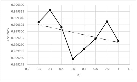
Figure 10.
Three-bay two-story framework with EEP2 semi-rigid connections. Accuracy vs. α0.
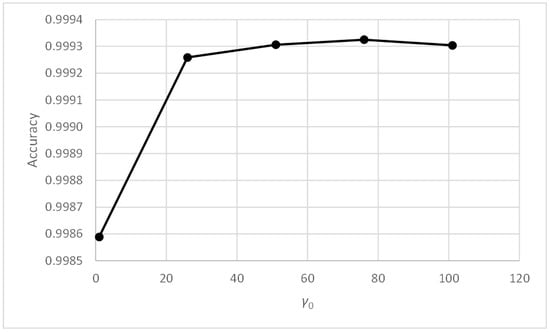
Figure 11.
Three-bay two-story framework with EEP2 semi-rigid connections. Accuracy vs. γ0.

Figure 12.
Three-bay two-story framework with EEP2 semi-rigid connections. Standard deviation vs. α0.
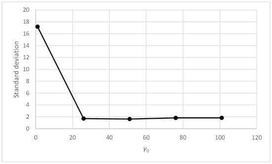
Figure 13.
Three-bay two-story framework with EEP2 semi-rigid connections. Standard deviation vs. γ0.
Figure 10 shows how the accuracy metric improves slightly when parameter α0 decreases. Figure 12 shows something similar occurring with the standard deviation metric, which does not exceed values of 1.83. Therefore, the PFAM is efficient and robust for values of α0 between 0.3 and 1.0.
Figure 11 and Figure 13 show that, for values of parameter γ0 above unity, the accuracy and standard deviation metrics give good and very similar values. Table 8 and Table 9 show that this effect appears with γ0 values above 10. Therefore, PFAM is efficient and robust for γ0 values between 10 and 100.
To better understand the behavior of the metrics with more detailed variations of parameters tc and m, an additional sensitivity analysis was performed with constant values of parameters β0 = 1, nt = 250, kmax = 100, α0 = 0.3, and γ0 = 76. The accuracy results are shown in Table 13, and the standard deviation results are shown in Table 14.
Table 13.
Three-bay two-story framework with EEP2 semi-rigid connections. Second sensitivity analysis for tc and m. Accuracy.
Table 14.
Three-bay two-story framework with EEP2 semi-rigid connections. Second sensitivity analysis for tc and m. Standard deviation.
If Table 6 and Table 7 (obtained with α0 = 1.0, γ0 = 10) are compared with Table 13 and Table 14 (obtained with α0 = 0.3, γ0 = 76), we can see that the shaded areas, with poor values of efficiency and robustness, are more extensive in Table 13 and Table 14. This demonstrates the interdependence among the parameters. Therefore, any sensitivity study needs to take this effect into account.
From the sensitivity analyses performed in this example, PFAM initially seems efficient and robust for the parameter values in Table 15. Nevertheless, these values were checked in another problem to study PFAM’s behavior and establish another level of robustness, namely that of the algorithm against changes in the problem.
Table 15.
Three-bay two-story framework with EEP2 semi-rigid connections. Optimum values of PFAM parameters.
Furthermore, parameters nt and kmax in Table 15 clearly depend on the problem. This is because each problem has a different number of variables, which affects the size of the design space. If the design space is large, sufficiently high nt values should be considered to ensure that the fireflies can capture enough information in the exploration phase. Likewise, sufficiently high kmax values must be taken into account so the algorithm can evolve from the exploration phase to the exploitation phase. The problem in which the connections between members of the structure are rigid, using only the necessary design variables X1, X2, X3, and X4 (see Table 2 and Table 3), has been considered in the same example to illustrate these ideas.
With rigid connections and initial constant values β0 = 1 m = 2, γ0 = 10, α0 = 1, and tc = 0.1, the values of the nt and kmax parameters were modified. The accuracy results are shown in Table 16, and the standard deviation results are shown in Table 17.
Table 16.
Three-bay two-story framework with rigid connections. Sensitivity analysis for nt and kmax. Accuracy.
Table 17.
Three-bay two-story framework with rigid connections. Sensitivity analysis for nt and kmax. Standard deviation.
In Table 16, the maximum accuracy values have been highlighted in bold, as have the minimum values of standard deviation in Table 17. The shaded areas in both figures correspond to the lowest efficiency (accuracy below 0.9) and robustness (standard deviation above 1000) values. The values of parameters nt = 30 and kmax = 100 gave good results and had a low computational cost, so they were chosen for the following sensitivity calculation.
With rigid connections and constant values β0 = 1, nt = 30, kmax = 100, γ0 = 10, and α0 = 1, the values of the tc and m parameters were modified. As previously carried out with nt and kmax, and because it was the first sensitivity calculation performed with parameters tc and m, wide ranges of both parameters were considered. The accuracy results are shown in Table 18, and the standard deviation results are shown in Table 19.
Table 18.
Three-bay two-story framework with rigid connections. Sensitivity analysis for tc and m. Accuracy.
Table 19.
Three-bay two-story framework with rigid connections. Sensitivity analysis for tc and m. Standard deviation.
In Table 18, the maximum accuracy values have been highlighted in bold, as have the minimum values of standard deviation in Table 19. Figure 14, Figure 15, Figure 16 and Figure 17 include the graphs of the accuracy and standard deviation means. These graphs show the sensitivity of both metrics to parameters m and tc. Some of the graphs also include linear regression analyses of the data, which helps detect trends in both metrics against changes in the value of the parameters.
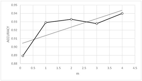
Figure 14.
Three-bay two-story framework with rigid connections. Accuracy vs. m.
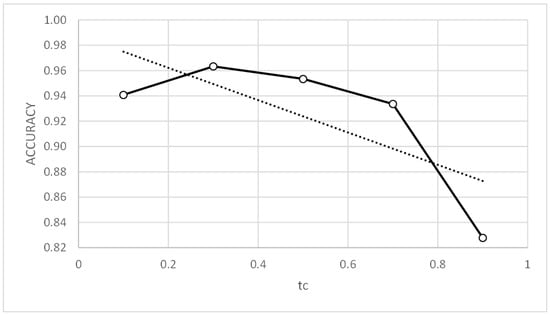
Figure 15.
Three-bay two-story framework with rigid connections. Accuracy vs. tc.
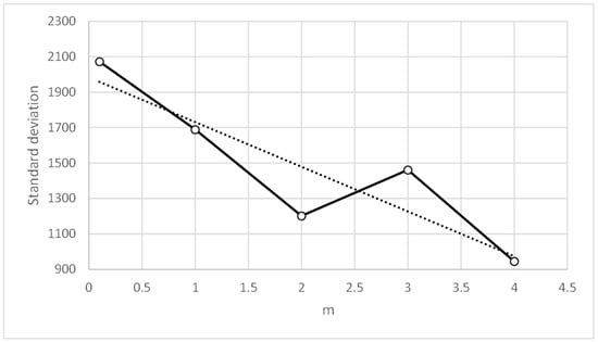
Figure 16.
Three-bay two-story framework with rigid connections. Standard deviation vs. m.
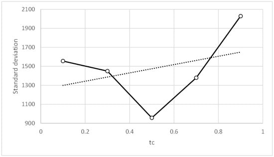
Figure 17.
Three-bay two-story framework with rigid connections. Standard deviation vs. tc.
Table 18 and Table 19 show that good and similar results were obtained for the metrics of parameter values tc = 0.1 to 0.7 and m = 1 to 4. However, Figure 14, Figure 15, Figure 16 and Figure 17 show that the means of the metrics improve for high values of parameter m and low values of parameter tc, the latter having the most influence on the results. For this reason, two sensitivity analyses were performed: (i) with parameter values tc = 0.3 and m = 2, and (ii) with parameter values tc = 0.1 and m = 4.
- First sensitivity analysis: with rigid connections and constant values β0 = 1, nt = 30, kmax = 100, tc = 0.3, and m = 2, the values of the α0 and γ0 parameters were modified. As previously carried out, and because it was the first sensitivity calculation performed with parameters α0 and γ0, wide ranges of both parameters were considered. The accuracy results are shown in Table 20, and the standard deviation results are shown in Table 21.
Table 20.
Three-bay two-story framework with rigid connections. First sensitivity analysis for α0 and γ0. Accuracy.
Table 20.
Three-bay two-story framework with rigid connections. First sensitivity analysis for α0 and γ0. Accuracy.
| γ0 | Mean | ||||||||
|---|---|---|---|---|---|---|---|---|---|
| 0.1 | 1 | 10 | 25 | 50 | 75 | 100 | |||
| α0 | 0.3 | 1.000000 | 0.946488 | 0.992191 | 0.910663 | 0.891969 | 0.758022 | 0.668462 | 0.881113 |
| 0.4 | 1.000000 | 0.967716 | 0.993883 | 0.882127 | 0.832489 | 0.786748 | 0.786933 | 0.892842 | |
| 0.5 | 1.000000 | 0.971335 | 0.992453 | 0.943934 | 0.753382 | 0.838944 | 0.921210 | 0.917323 | |
| 0.6 | 0.971560 | 0.952837 | 0.898089 | 0.844372 | 0.708637 | 0.773464 | 0.598494 | 0.821065 | |
| 0.7 | 0.997763 | 0.993318 | 0.933460 | 0.909359 | 0.779504 | 0.788907 | 0.662411 | 0.866389 | |
| 0.8 | 0.997763 | 0.973706 | 0.922725 | 0.923220 | 0.887281 | 0.861669 | 0.754091 | 0.902922 | |
| 0.9 | 0.970565 | 0.966832 | 0.956470 | 0.974998 | 0.883387 | 0.700241 | 0.827291 | 0.897112 | |
| 1.0 | 0.939673 | 0.952912 | 0.955308 | 0.911318 | 0.808622 | 0.770159 | 0.680694 | 0.859812 | |
| mean | 0.984665 | 0.965643 | 0.955572 | 0.912499 | 0.818159 | 0.784769 | 0.737448 | ||
Table 21.
Three-bay two-story framework with rigid connections. First sensitivity analysis for α0 and γ0. Standard deviation.
Table 21.
Three-bay two-story framework with rigid connections. First sensitivity analysis for α0 and γ0. Standard deviation.
| γ0 | Mean | ||||||||
|---|---|---|---|---|---|---|---|---|---|
| 0.1 | 1 | 10 | 25 | 50 | 75 | 100 | |||
| α0 | 0.3 | 0.00 | 1128.45 | 131.15 | 1532.62 | 1684.33 | 2990.43 | 3459.81 | 1560.97 |
| 0.4 | 0.00 | 868.15 | 94.18 | 1763.05 | 2588.30 | 4499.15 | 3664.25 | 1925.30 | |
| 0.5 | 0.00 | 761.60 | 97.77 | 1141.50 | 3045.85 | 2183.85 | 638.44 | 1124.15 | |
| 0.6 | 749.05 | 1244.95 | 2289.27 | 3165.81 | 4131.11 | 2993.27 | 5184.88 | 2822.62 | |
| 0.7 | 62.20 | 101.90 | 1747.11 | 1915.66 | 3609.77 | 2567.04 | 4039.21 | 2006.13 | |
| 0.8 | 62.20 | 686.37 | 2161.60 | 1170.22 | 1555.39 | 1829.78 | 3129.82 | 1513.62 | |
| 0.9 | 683.55 | 856.40 | 1024.49 | 231.44 | 1627.07 | 3962.12 | 2520.01 | 1557.87 | |
| 1.0 | 1491.07 | 1062.74 | 849.50 | 1365.04 | 2745.92 | 3131.86 | 3486.90 | 2019.00 | |
| mean | 381.01 | 838.82 | 1049.38 | 1535.67 | 2623.47 | 3019.69 | 3265.41 | ||
In Table 20, the maximum accuracy values have been highlighted in bold, as have the minimum values of standard deviation in Table 21. Parameter γ0 values above 10 produce poor results regardless of the value of parameter α0. The best results were obtained in the γ0 range [0.1, 10] and the α0 range [0.3, 0.5]. Figure 18, Figure 19, Figure 20 and Figure 21 include the graphs of the accuracy and standard deviation means. These graphs show the sensitivity of both metrics to parameters γ0 and α0. Some of the graphs also include linear regression analyses on the data, which helps detect trends in both metrics against changes in the value of the parameters.
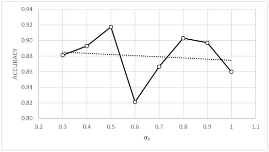
Figure 18.
Three-bay two-story framework with rigid connections. First sensitivity analysis. Accuracy vs. α0.
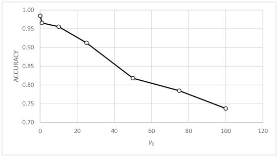
Figure 19.
Three-bay two-story framework with rigid connections. First sensitivity analysis. Accuracy vs. γ0.
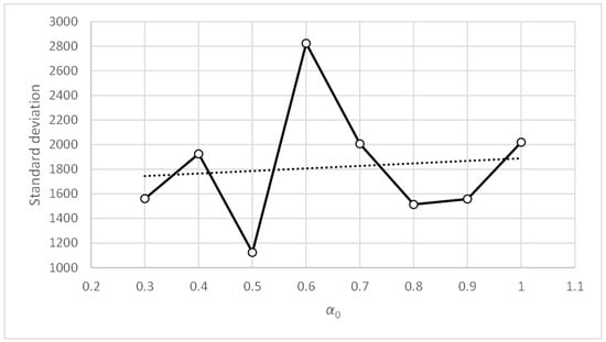
Figure 20.
Three-bay two-story framework with rigid connections. First sensitivity analysis. Standard deviation vs. α0.
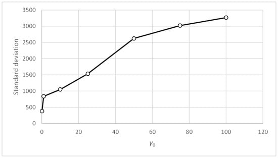
Figure 21.
Three-bay two-story framework with rigid connections. First sensitivity analysis. Standard deviation vs. γ0.
Figure 18 shows how the accuracy metric improves slightly when parameter α0 decreases. Figure 20 shows similar behavior with the standard deviation metric. Figure 19 and Figure 21 show that the accuracy and standard deviation values are reasonably good and quite similar for values of parameter γ0 below 25.
- ii.
- Second sensitivity analysis: with rigid connections and constant values β0 = 1, nt = 30, kmax = 100, tc = 0.1, and m = 4, the values of the α0 and γ0 parameters were modified. As previously carried out, wide ranges of parameters α0 and γ0 were considered. The accuracy results are shown in Table 22, and the standard deviation results are shown in Table 23.
Table 22. Three-bay two-story framework with rigid connections. Second sensitivity analysis for α0 and γ0. Accuracy.
Table 23. Three-bay two-story framework with rigid connections. Second sensitivity analysis for α0 and γ0. Standard deviation.
In Table 22, the maximum accuracy values have been highlighted in bold, as have the minimum values of standard deviation in Table 23. In terms of parameter γ0, values above 75 and in the α0 range of [0.7, 1.0] produce poor results. For the rest of the α0 and γ0 values, a dispersion of poor metric values was observed. Figure 22, Figure 23, Figure 24 and Figure 25 include the graphs of the accuracy and standard deviation means. These graphs show the sensitivity of both metrics to parameters γ0 and α0. Some of the graphs also include linear regression analyses on the data, which helps detect trends in both metrics against changes in the value of the parameters.
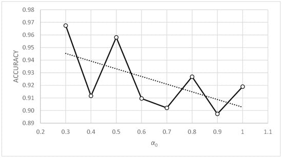
Figure 22.
Three-bay two-story framework with rigid connections. Second sensitivity analysis. Accuracy vs. α0.
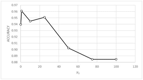
Figure 23.
Three-bay two-story framework with rigid connections. Second sensitivity analysis. Accuracy vs. γ0.

Figure 24.
Three-bay two-story framework with rigid connections. Second sensitivity analysis. Standard deviation vs. α0.
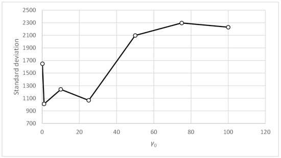
Figure 25.
Three-bay two-story framework with rigid connections. Second sensitivity analysis. Standard deviation vs. γ0.
Figure 22 shows how the accuracy metric improves when parameter α0 decreases. Figure 24 shows similar behavior with the standard deviation metric. Figure 23 and Figure 25 show that the accuracy and standard deviation metrics are reasonably good and have very similar values for parameter γ0 in the range [1,25].
Comparing Figure 18, Figure 20, Figure 22 and Figure 24, showing the evolution of the accuracy and standard deviation metrics with α0, we can see that the sensitivity of both metrics with α0 increases when the value of tc is reduced. Better results are also obtained from the metrics for values of tc = 0.1. Finally, the best results are obtained for α0 values in the range [0.3, 0.5] for both tc = 0.1 and tc = 0.3.
Comparing Figure 19, Figure 21, Figure 23 and Figure 25, showing the evolution of the accuracy and standard deviation metrics with γ0, we can see that the sensitivity of both metrics with γ0 increases when the value of tc is reduced. Better results are also obtained from the metrics for values of tc = 0.1. Finally, the best results are obtained for γ0 values in the range [1,25] for tc = 0.1 and for γ0 values in the range [0.1, 10] for tc = 0.3.
To better understand the behavior of the metrics with more detailed variations of parameters tc and m, an additional sensitivity analysis was conducted with constant values for parameters β0 = 1, nt = 30, kmax = 100, α0 = 0.3, and γ0 = 0.1. The accuracy results are shown in Table 24, and the standard deviation results are shown in Table 25.
Table 24.
Three-bay two-story framework with rigid connections. Second sensitivity analysis for tc and m. Accuracy.
Table 25.
Three-bay two-story framework with rigid connections. Second sensitivity analysis for tc and m. Standard deviation.
If Table 18 and Table 19 (obtained with α0 = 1.0, γ0 = 10) are compared with Table 24 and Table 25 (obtained with α0 = 0.3, γ0 = 0.1), we can see that the shaded areas, corresponding to poor values of efficiency and robustness, are more extensive in Table 18 and Table 19. This, again, demonstrates the interdependence among the parameters.
As a result of the sensitivity analyses performed in this example, PFAM initially seems efficient and robust for the parameter values in Table 26.
Table 26.
Three-bay two-story framework with rigid connections. Optimum values of PFAM parameters.
If we take into account the parameter values included in Table 15 (EEP2 semi-rigid connections) and Table 26 (rigid connections) and look for the intersection or common values in these tables for a three-bay two-story framework, PFAM seems efficient and robust for the parameter values included in Table 27.
Table 27.
Three-bay two-story framework with rigid or EEP2 semi-rigid connections. Optimum values of PFAM parameters.
4.1.2. Parameter Control for the Three-Bay Two-Story Framework
As parameters tc and α0 are closely related, and both define a strategy for moving from the exploration phase to the exploitation phase that is unique from start to finish, they were considered constant in the PCPFAM procedure proposed in this work. The value of tc = 0.1 was adopted to guarantee a sufficient margin of passage from the exploration phase to the exploitation phase. The value of α0 = 1.0 was also chosen so the subpopulations could initially explore the entire design space in the exploration phase regardless of the values of the other parameters. Furthermore, the value of 2 was given to parameter m, as it was found to have little effect on the results. However, parameter nt depends on the number of variables considered in each problem, affecting the entire process as tc and α0 do, so the value found in the previous sensitivity analysis was used. Finally, the proposed PCPFAM procedure was applied to the γ parameter, which greatly affected the efficiency and robustness results.
Considering both semi-rigid connections EEP2 and rigid connections, and constant values β0 = 1, kmax = 100, tc = 0.1, α0 = 1.0, and m = 2, the PCPFAM procedure was applied to parameter γ. The range of values for γ was [1, 50]. The evolution of parameter γ in each subpopulation for a run is shown in Figure 26. The accuracy and standard deviation results are shown in Table 28, and there were 50 independent runs.
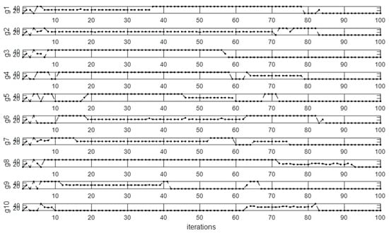
Figure 26.
Three-bay two-story framework with rigid connections. PCPFAM. Evolution of parameter γ.
Table 28.
Three-bay two-story framework. PCPFAM. Accuracy and Standard deviation.
4.2. Three-Bay Ten-Story Framework
The three-bay ten-story structure shown in Figure 27 and Figure 28 has been previously studied by Xu and Grierson [34], Foley and Schinler [35], Kameshki and Saka [36], Ali et al. [33], and Sánchez-Olivares and Tomás [21]. Figure 27 shows the geometry of the structure and the loads considered: floor dead load (Df); floor live load (Lf); roof dead load (Dr); roof live load (Lr); and wind load (W). Taking these loads into account, two load combinations were considered:
I: (1.0Df + 1.0Dr + 0.4Lf + 0.4Lr + 0.5W),
II: (1.2Df + 1.2Dr + 0.5Lf + 0.5Lr + 1.3W).

Figure 27.
Geometry and loads for the three-bay ten-story framework.
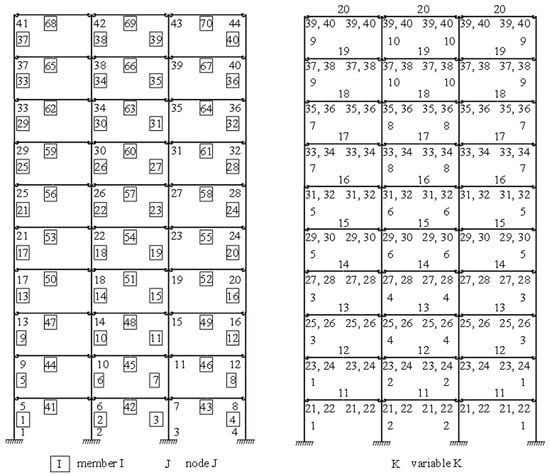
Figure 28.
Nodes, members, and design variables for the three-bay ten-story framework.
Figure 28 shows the numbering used for the nodes, members, and design variables. The expressions from 6 to 19 were considered following the requirements of Eurocode 3 [24]. The columns and beams have HEB and IPE steel shapes, respectively, and the design variables are included in Table 29.
Table 29.
Design variables for the three-bay ten-story framework.
Steel S235 with Young’s modulus E = 210 GPa, fy = 235 MPa yield strength, and a resistance factor of γm = 1.0 was the material chosen for the steel shapes in the members and the steel plates in the semi-rigid connections. The ultimate tensile strength and resistance factor for the bolts in the semi-rigid connections were fub = 800 MPa and γm = 1.25, respectively. The material cost of the steel was set at C = 1.6 EUR/kg. The cost of the rigid connections in the frame was calculated assuming a fixity factor of 0.964 [21]. To model the behavior of extended end-plates with stiffened column flange semi-rigid connections (EEP1) and extended end-plates without stiffened column flange semi-rigid connections (EEP2), the Component Method was used.
The PFAM algorithm was run 100 times using different random seeds so the best-generated solution would be chosen as the optimal design solution. Ten subpopulations were considered in all the runs. The values of the parameters used in the PFAM algorithm were the following: β0 = 1 m = 2, γ0 = 10, α0 = 1, nt = 1000, kmax = 100, and tc = 0.1. Figure 29 shows the evolutions of the objective functions in one of the 100 executions with rigid connections and EEP1 and EEP2 semi-rigid connections. The optimal design solutions obtained by Ali et al. [33] and using the PFAM algorithm proposed in this work are included in Table 30.
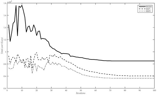
Figure 29.
Objective function evolutions using PFAM for the three-bay ten-story framework and considering rigid and semi-rigid connections EEP1 and EEP2.
Table 30.
Final designs for the three-bay ten-story framework.
4.2.1. Parameter Tuning in PFAM for the Three-Bay Ten-Story Framework
To study PFAM’s performance for the three-bay ten-story framework, a similar sensitivity analysis to the previous one was performed considering different values for a pair of parameters.
With EEP2 semi-rigid connections, and initial constant values β0 = 1, m = 2, γ0 = 10, α0 = 1, and tc = 0.1, the values of the nt and kmax parameters were modified. Based on the results from the previous example, a wide range of values for the nt parameter and only three values for the kmax parameter were considered. There were 50 independent runs. The accuracy results are shown in Table 31, and the standard deviation results are shown in Table 32.
Table 31.
Three-bay ten-story framework with EEP2 semi-rigid connections. Sensitivity analysis for nt and kmax. Accuracy.
Table 32.
Three-bay ten-story framework with EEP2 semi-rigid connections. Sensitivity analysis for nt and kmax. Standard deviation.
In Table 31, the maximum accuracy values have been highlighted in bold, as have the minimum values of standard deviation in Table 32. The values of parameters nt = 1000 and kmax = 100 gave good results and had a low computational cost, so they were chosen for the following sensitivity calculation.
With EEP2 semi-rigid connections, and constant values β0 = 1, nt = 1000, kmax = 100, γ0 = 10, and α0 = 1, the values of the tc and m parameters were modified. Taking the information above into account, sufficiently wide ranges of the tc and m parameters were considered. The accuracy results are shown in Table 33, and the standard deviation results are shown in Table 34.
Table 33.
Three-bay ten-story framework with EEP2 semi-rigid connections. Sensitivity analysis for tc and m. Accuracy.
Table 34.
Three-bay ten-story framework with EEP2 semi-rigid connections. Sensitivity analysis for tc and m. Standard deviation.
In Table 33, the maximum accuracy values have been highlighted in bold, as have the minimum values of standard deviation in Table 34. Parameter values tc = 0.1 and m = 1, or m = 2 had good and similar results, so they were chosen for the following sensitivity calculation.
With EEP2 semi-rigid connections, and constant values β0 = 1, nt = 1000, kmax = 100, tc = 0.1, and m = 1, the values of the α0 and γ0 parameters were modified. Taking this above information into account, sufficiently wide ranges of the α0 and γ0 parameters were considered. The accuracy results are shown in Table 35, and the standard deviation results are shown in Table 36.
Table 35.
Three-bay ten-story framework with EEP2 semi-rigid connections. Sensitivity analysis for α0 and γ0. Accuracy.
Table 36.
Three-bay ten-story framework with EEP2 semi-rigid connections. Sensitivity analysis for α0 and γ0 Standard deviation.
In Table 35, the maximum accuracy values have been highlighted in bold, as have the minimum values of standard deviation in Table 36. Parameter γ0 values below 1 produced poor results regardless of the value of parameter α0.
In summary, after performing these sensitivity analyses, the following was observed:
- (i)
- the selected values of parameters nt = 1000 and kmax = 100 produced good metric results with low computational cost;
- (ii)
- parameter tc affected the exploration and exploitation phases of the algorithm, obtaining good metric values when values of parameter tc of around 0.1 were adopted;
- (iii)
- m values close to the unit produced good metric values for low tc values; and
- (iv)
- the values of parameter γ0 greater than the unit produced good metric values, with α0 in the range [0.3, 1.0].
As a result of the sensitivity analyses performed in this example, PFAM initially seems efficient and robust for the parameter values in Table 37. However, these values have been checked in another problem to study PFAM’s behavior and establish another level of robustness, namely that of the algorithm against changes in the problem.
Table 37.
Three-bay ten-story framework with EEP2 semi-rigid connections. Optimum values of PFAM parameters.
As in the previous example, a problem with rigid connections between members of the structure has been considered, for which only the design variables X1 to X20 are necessary (see Table 29 and Table 30).
With rigid connections, and the initial constant values β0 = 1 m = 2, γ0 = 10, α0 = 1, and tc = 0.1, the nt and kmax parameter values were modified. The accuracy results are shown in Table 38, and the standard deviation results are shown in Table 39.
Table 38.
Three-bay ten-story framework with rigid connections. Sensitivity analysis for nt and kmax. Accuracy.
Table 39.
Three-bay ten-story framework with rigid connections. Sensitivity analysis for nt and kmax. Standard deviation.
In Table 38, the maximum accuracy values have been highlighted in bold, as have the minimum values of standard deviation in Table 39. The shaded areas in both tables correspond to the lowest values of efficiency and robustness. The values of parameters nt = 450 and kmax = 100 gave good results and had a low computational cost, so they were chosen for the following sensitivity calculation.
Considering rigid connections, and constant values β0 = 1, nt = 450, kmax = 100, γ0 = 10, and α0 = 1, the tc and m parameter values were modified. The accuracy results are shown in Table 40, and the standard deviation results are shown in Table 41.
Table 40.
Three-bay ten-story framework with rigid connections. Sensitivity analysis for tc and m. Accuracy.
Table 41.
Three-bay ten-story framework with rigid connections. Sensitivity analysis for tc and m. Standard deviation.
In Table 40, the maximum accuracy values have been highlighted in bold, as have the minimum values of standard deviation in Table 41. The ranges of both parameters tc and m produced good and similar results. Figure 30 and Figure 31 include the graphs of the accuracy and standard deviation means. These graphs show the sensitivity of both metrics to parameters m and tc. Some of the graphs also include linear regression analyses of the data, which helps detect trends in both metrics against changes in the value of the parameters.
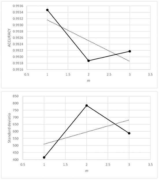
Figure 30.
Three-bay ten-story framework with rigid connections. Accuracy vs. m and standard deviation vs. m.
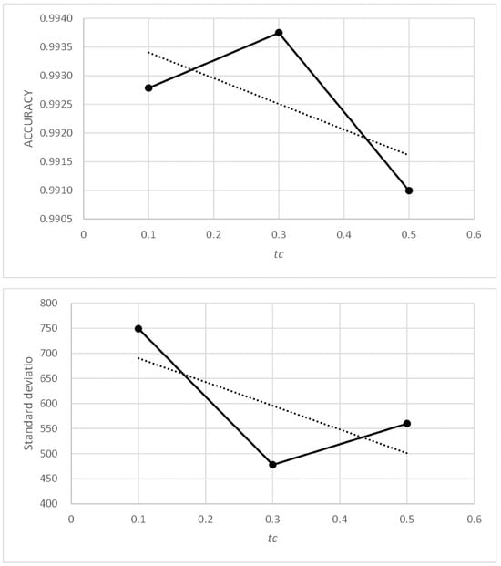
Figure 31.
Three-bay ten-story framework with rigid connections. Accuracy vs. tc and standard deviation vs. tc.
Table 40 and Table 41 and Figure 30 and Figure 31 show that the parameter values tc = 0.3 and m = 1 gave the best results, so they were chosen for the following sensitivity calculation.
Considering rigid connections, and the constant values β0 = 1, nt = 450, kmax = 100, tc = 0.3, and m = 1, the values of the α0 and γ0 parameters were modified. The results obtained for accuracy are shown in Table 42. The results obtained for standard deviation are shown in Table 43.
Table 42.
Three-bay ten-story framework with rigid connections. Sensitivity analysis for α0 and γ0. Accuracy.
Table 43.
Three-bay ten-story framework with rigid connections. Sensitivity analysis for α0 and γ0. Standard deviation.
In Table 42, the maximum accuracy values have been highlighted in bold, as have the minimum values of standard deviation in Table 43. The ranges of both parameters α0 and γ0 produced good and similar results.
As a result of the sensitivity analyses performed in this example, PFAM initially seems efficient and robust for the parameter values in Table 44.
Table 44.
Three-bay ten-story framework with rigid connections. Optimum values of PFAM parameters.
If we take into account the values of the parameters in Table 37 (EEP2 semi-rigid connections) and Table 44 (rigid connections), and look for the intersection or common values of both tables for the three-bay two-story framework, we can conclude that PFAM seems efficient and robust for the parameter values in Table 45.
Table 45.
Three-bay ten-story framework with rigid or EEP2 semi-rigid connections. Optimum values of PFAM parameters.
4.2.2. Parameter Control for the Three-Bay Ten-Story Framework
As in the previous example, parameters tc, α0, and m were considered constants in the parameter control procedure (PCPFAM) proposed in this work. The proposed PCPFAM procedure on γ was taken into account.
Considering both semi-rigid connections EEP2 and rigid connections, and the constant values β0 = 1, kmax = 100, tc = 0.1, α0 = 1.0, and m = 2, the PCPFAM procedure was applied to parameter γ. The range of values for γ was [1, 50]. The evolution of parameter γ in each subpopulation for a run is shown in Figure 32. The accuracy and standard deviation results are shown in Table 46. There were 50 independent runs.
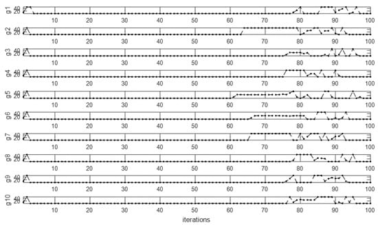
Figure 32.
Three-bay ten-story framework with rigid connections. PCPFAM. Evolution of parameter γ.
Table 46.
Three-bay ten-story framework. PCPFAM. Accuracy and Standard deviation.
4.3. Analysis and Discussion of the Results
In the first example, an extensive sensitivity analysis was carried out using PFAM. Different values were considered for a couple of parameters within extensive ranges, establishing those obtaining better metrics as tuned values. With tuned values, another pair of parameters were modified. This procedure was carried out several times. As expected, a strong interdependence among the parameter values was observed because the tuned values for a couple of them depended on the constant values chosen for the rest of the parameters.
Therefore, adjusting parameters through simple procedures, such as the one shown here, is an arduous task that requires time and has a high computational cost.
In the second example, a less extensive sensitivity analysis was carried out, as it was only intended to check the robustness of PFAM when different design cases are considered.
At the end of the process, small differences were found in the tuned values of parameters tc, α0, and m when comparing the results obtained in both examples with rigid and semi-rigid connections. However, greater differences were found in the tuned values of parameters γ0 and nt. This situation could create uncertainty for future users when applying PFAM to the design of a new structure that differs considerably from previously designed structures.
The PCPFAM selects the values of one or several parameters that maximize changes in landscape Fi during the design process. However, the parameters can be classified into two groups: those that can change during the process (β0, α, γ, m) and those chosen at the beginning of the process that do not change during the process (tc, nt, kmax). PCPFAM can only act on the former.
The uncertainty in the choice of γ was resolved using PCPFAM. After having carried out the different sensitivity analyses with PFAM, some tuned and untuned values of the rest of the parameters were adopted in PCPFAM with a constant value during the process. The results showed that the algorithm obtained good metrics when parameter γ was changeable during the design process, which made the algorithm more robust.
However, there is still uncertainty in the choice of parameter nt. The adjusted values obtained through the sensitivity analyses carried out with PFAM show that nt depends on nv, with very different values in each of the examples.
To eliminate the uncertainty in the choice of parameter nt, its dependence on nv was studied. First, the total number of possible designs (TNPD) in the examples was calculated as variations with repetitions of ne elements taken from nve to nve. In the two examples, 24 (ne = 24) HEB steel shapes were considered for the columns and 18 (ne = 18) IPE steel shapes for the beams. When there were semi-rigid connections in the examples, 10 (ne = 10) different types of steel bolts and 12 (ne = 12) different types of steel end-plates were also considered. In the examples, nve is the number of variables used for the HEB and IPE shapes and the steel bolts and steel end-plates (see Table 2, Table 3, Table 29 and Table 30). Thus, the TNPD in all the examples are included in Table 47. As can be seen, ne does not vary in the different cases, and nve does. Furthermore, the TNPD is a large number in all the cases. Therefore, it seems reasonable to use logarithms, although doubts arise about the base to use. In Table 47, base be gives the same TNPD previously obtained when it is raised to the number of variables in each case.
Table 47.
TNPD and be.
Thus, when calculating the logarithms, a single value, which was the average of the four values of be included in Table 47 and is equal to 17.554979964, was used for the base of be. Table 48 includes the minimum populations nt (minpop) that yielded the most precise results with minimal computational cost with kmax = 100 for each case (see Table 4, Table 5, Table 16, Table 17, Table 31, Table 32, Table 38 and Table 39). Likewise, the TNPD logarithms have been included for each case using the same base be = 17.554979964.
Table 48.
Calculation of logarithms over TNPD, nv, and minpop.
The third column of Table 48 shows that the logarithm calculated in each case was close to the number of variables nv considered (4, 12, 20, and 40). This is evident from looking at the calculations performed. Figure 33 shows minpop on the ordinate axis and nv on the abscissa axis. Likewise, the Least-Square Regression Line is included.

Figure 33.
minpop vs. nv.
Figure 33 shows the good fit obtained (R2 = 0.9997496). The calculations carried out using logarithms remind us of the concept of entropy S, which is a measure of the disorder or randomness of the system. In certain fields of knowledge, when information I is extracted from a system, entropy S is reduced [37,38,39]. Thus, the entropy S of a design space with volume TNPD, and the information I that PFAM and PCPFAM extract from it, are related (S ≥ S − I ≥ 0). In this context, minpop could be defined as the minimum or sufficient number of fireflies that PFAM or PCPFAM requires in the design process to provide enough information for a valid design. Since an algorithm can be defined as an information management tool, if the information minpop that the algorithm works with is sufficient, the difference S − I is a small enough value to obtain good metrics.
Finally, using the formula of the Least-Square Regression Line included in Figure 33, a simple expression resolving the uncertainty in the choice of nt is proposed. The estimated minimum population estminpop, as a function of nv, can be obtained using the following expression:
Expression (66), applied to values of nv = 4, 12, 20, and 40, provides the values of estminpop included in Figure 34. In addition, Figure 34 includes values of minpop and the Least-Square Regression Line.

Figure 34.
estminpop vs. minpop.
5. Conclusions
In this work, a numerical method for the optimal detailed design of steel frames based on a FA has been studied and proposed. The main objective has been to make the method sufficiently efficient and robust. The algorithm has been parallelized to reduce execution times, and a migration strategy has been implemented to allow information to be transferred among subpopulations, avoiding biases. An extensive sensitivity analysis of the algorithm has allowed knowledge about its performance to be extracted. Additionally, a variant of the algorithm has been proposed that implements a parameter control strategy. This variant has been tested on the parameter that most affects performance based on the information from the previous sensitivity analysis. Finally, a study demonstrating the near dependence between one of the parameters and the number of variables considered in the examples has been carried out. Two examples of steel structures, which have been extensively studied by other authors, have served to verify the efficiency and robustness of the optimal design method proposed.
The following conclusions can be drawn:
- The sensitivity of the PFAM algorithm is higher for changes in parameters tc, γ0, and nt than for changes in parameters α0, m, and kmax.
- As expected, a close dependence between parameters tc, α0, γ0, and m has been detected. Changes in the value of one produce changes in the optimal tuned values of the rest of them.
- The optimal tuned values of the parameters are different when considering EEP2 semi-rigid connections (SRC) or rigid connections (RC). The optimal tuned values somewhat affected are those related to parameters tc (SRC: [0.1, 0.3]; RC: [0.1, 0.5]), α0 (SRC: [0.3, 1.0]; RC: [0.3, 0.5]), γ0 (SRC: [10, 25]; RC: [0.1, 25]), and m (SRC: [1, 2]; RC: [1, 3]). The most affected optimal tuned values are those related to parameter nt (SRC: [250, 1000]; RC: [30, 450]).
- If the intersection between the above somewhat affected optimal tuned values is considered, it is concluded that the optimal tuned values are the following: tc ⸦ [0.1, 0.3]; α0 ⸦ [0.3, 0.5]; γ0 ⸦ [10, 25]; and m ⸦ [1, 2].
- The value of parameter kmax = 100 produces quite satisfactory results with a lower computational cost in all the cases considered.
- The sensitivity study does not allow an interval of optimal tuned values for the parameter nt independent of the problem to be determined.
- Considering different cases with constant values of some parameters, β0 = 1, kmax = 100, tc = 0.1, α0 = 1.0, and m = 2, all of them non-optimal and with a range of values for γ of the interval [1, 50], the PCPFAM procedure produces results as satisfactory as those obtained with the PFAM procedure and with optimal tuned values of the parameters. The fact that parameter γ varies in the interval [1, 50], maximizing the fitness landscape, compensates for not choosing optimal tuned values of other parameters, which makes PCPFAM more robust than PFAM.
- PCPFAM can only act on parameters β0, α, γ, and m, which may change during the design process, but not on parameters tc, nt, and kmax, which remain constant. Among the latter, nt is the one that most affects the algorithm’s performance. Therefore, PCPFAM cannot eliminate the uncertainty in the choice of parameter nt.
- The optimal tuned values of the nt parameter (minpop), found in the sensitivity analysis with PFAM, were very different and depended greatly on the case considered. The study was able to determine that parameter nt depends mainly on the number of variables nv considered in each case.
- Once the dependence of parameter nt, with respect to the number of variables nv, was detected, a Least-Square regression adjustment was made with the optimal tuned values minpop of parameter nt and the number of variables nv. A simple expression, which is easy to remember, removes the uncertainty for nt, giving it a value (estminpop) that is a function of the number of variables nv in the problem.
The proposed method can be used in engineering offices to obtain optimal detailed designs in a reasonable time. To achieve this, simple models can first be defined, such as those that consider rigid connections. After analysis with commercial software, the combinations of decisive loads in the design in ultimate limit states and serviceability limit states are detected. Finally, these actions are included in the proposed method, and the detailed optimal design is obtained. This procedure is necessary, since only one combination of loads has been considered in this study.
We should highlight that the proposed method is limited to planar structures. Therefore, it does not include the effect of node rotations on elements connected perpendicularly to the plane of the structure. Furthermore, it only considers static loads. These limitations serve to define future improvements to the proposed method.
Author Contributions
Conceptualization, A.T. and G.S.-O.; methodology and algorithm implementation, G.S.-O. and S.G.-A.; checking the results, A.T. and G.S.-O.; writing—original draft preparation, S.G.-A. and A.T.; writing—review and editing, S.G.-A. and A.T. All authors have read and agreed to the published version of the manuscript.
Funding
This research received no external funding.
Data Availability Statement
The data presented in this study are available on request from the corresponding author.
Conflicts of Interest
The authors declare no conflict of interest.
Appendix A
Below are the pseudo-codes and MATLAB® function files (ffa_mincon.m; factor_alpha.m; ffa_move.m; findlimits.m; escala.m; param_intrp.m) used for this research:

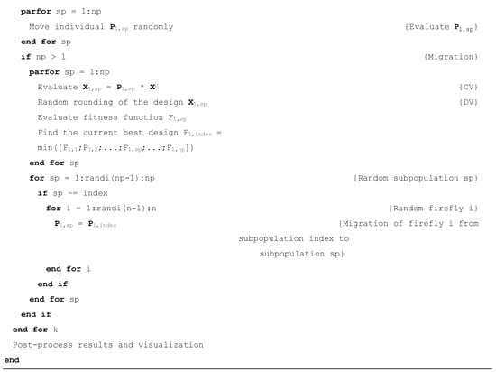
Figure A1.
Pseudo-code of PFAM.
Figure A1.
Pseudo-code of PFAM.
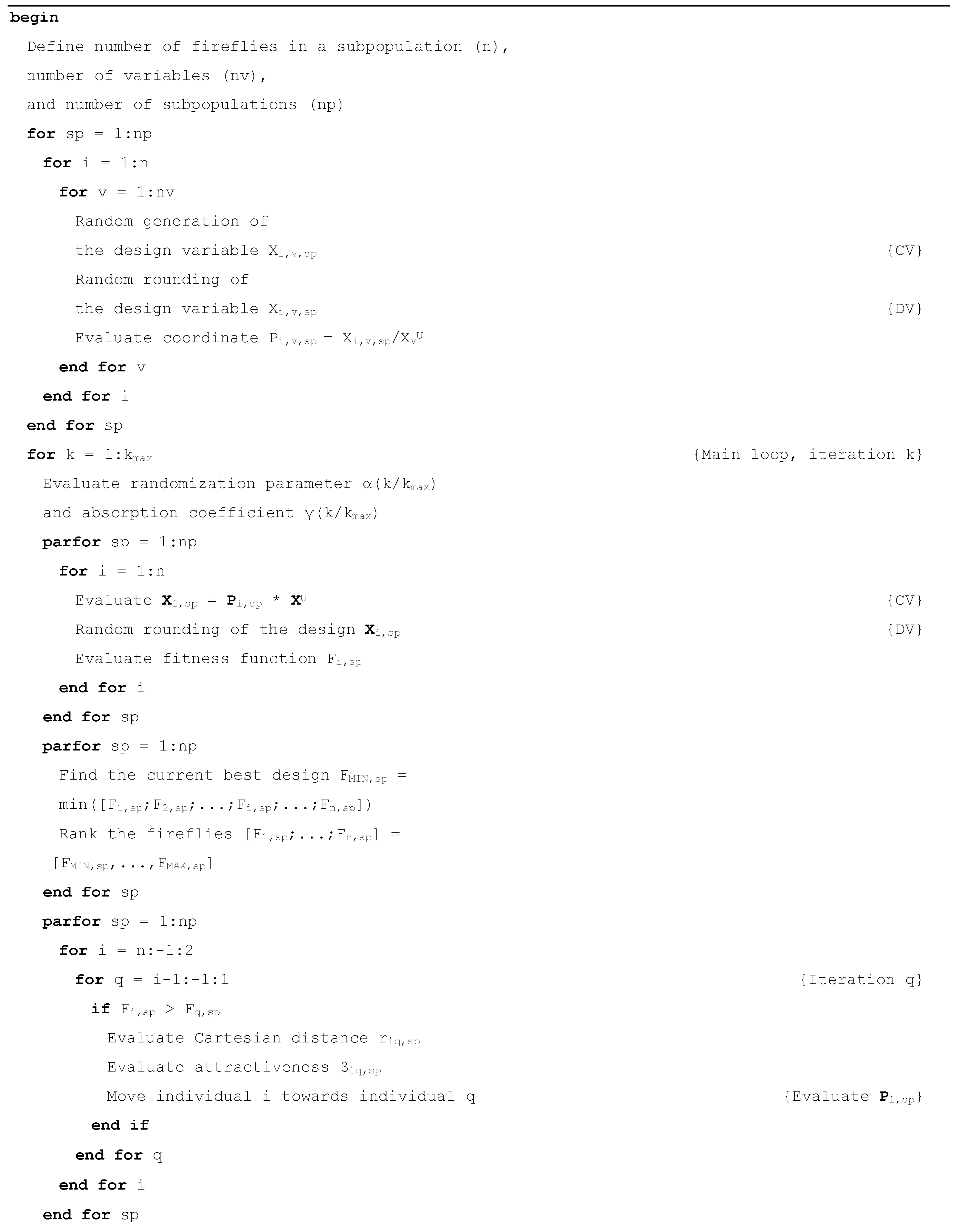
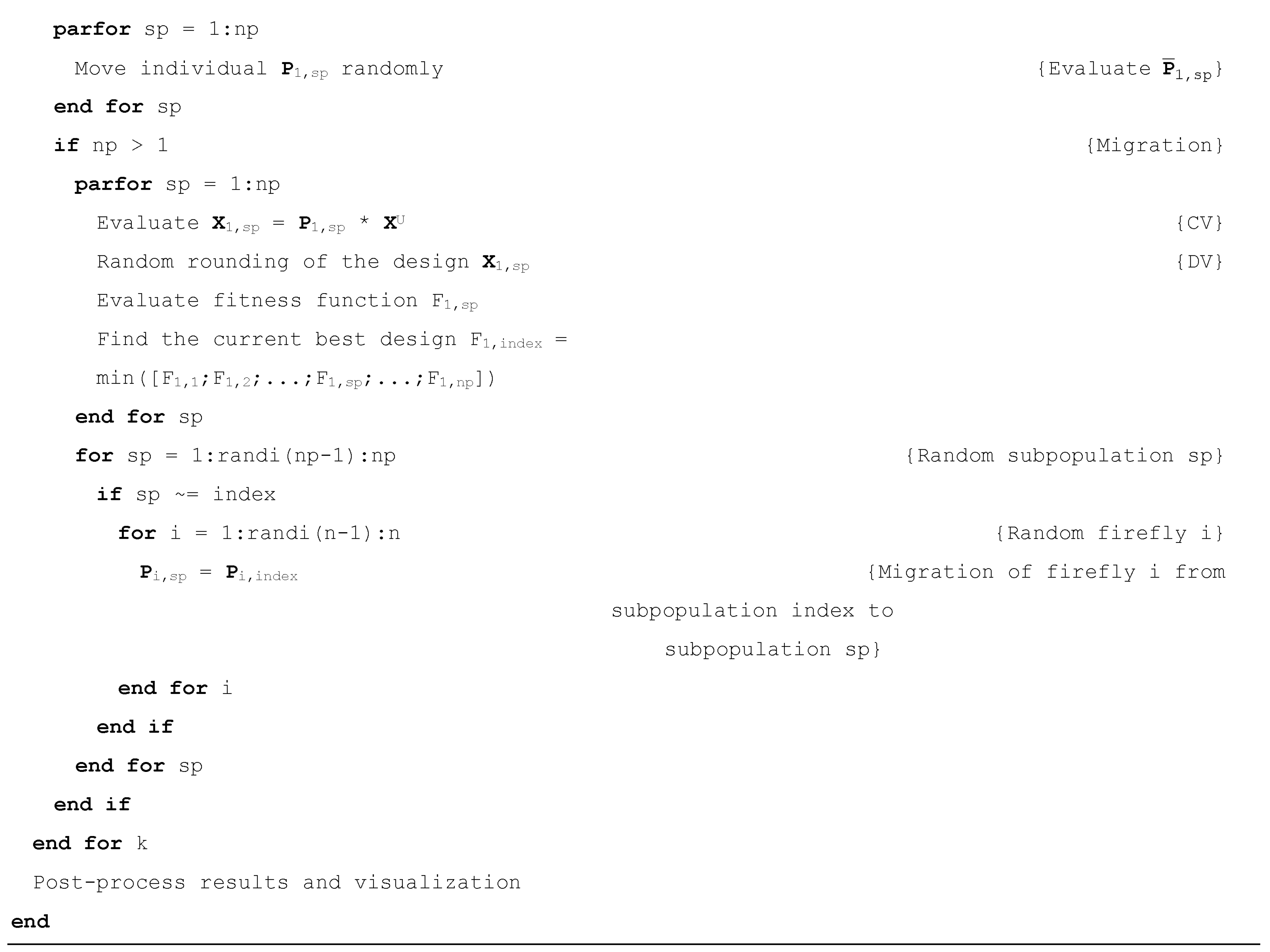

Figure A2.
Pseudo-code of PCPFAM.
Figure A2.
Pseudo-code of PCPFAM.

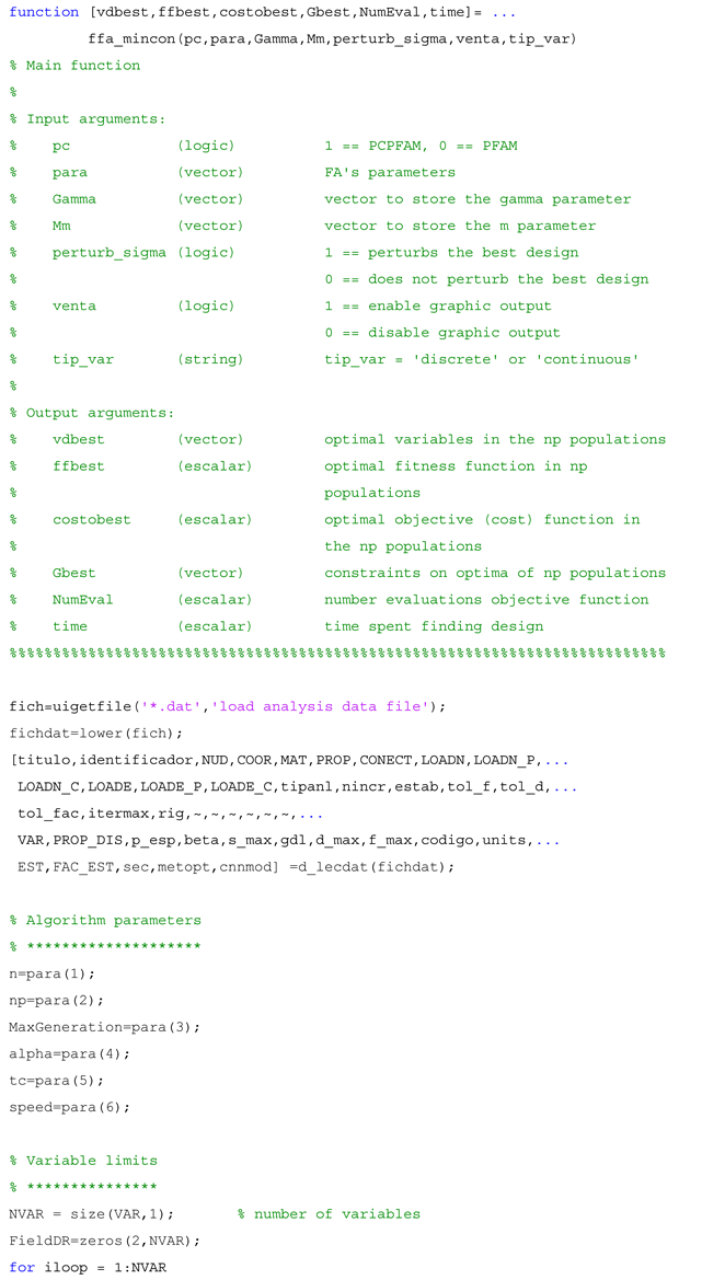
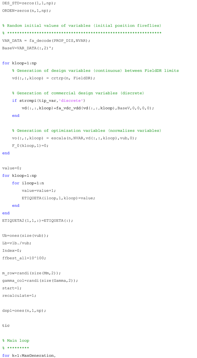
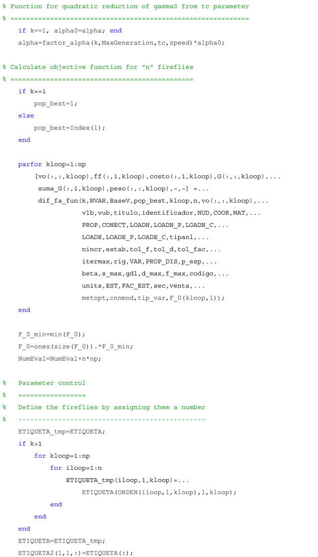
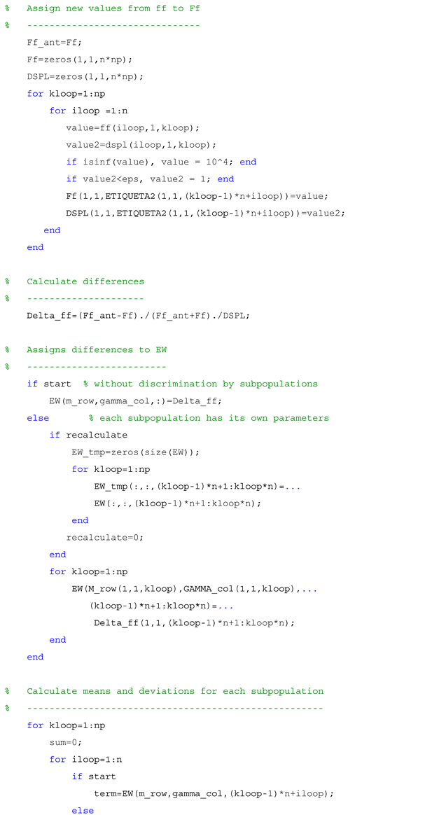
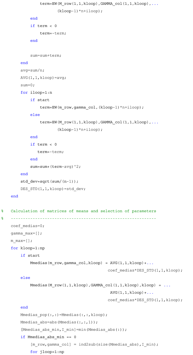
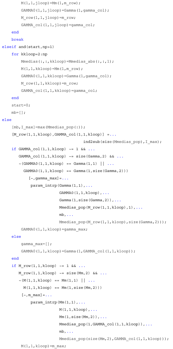
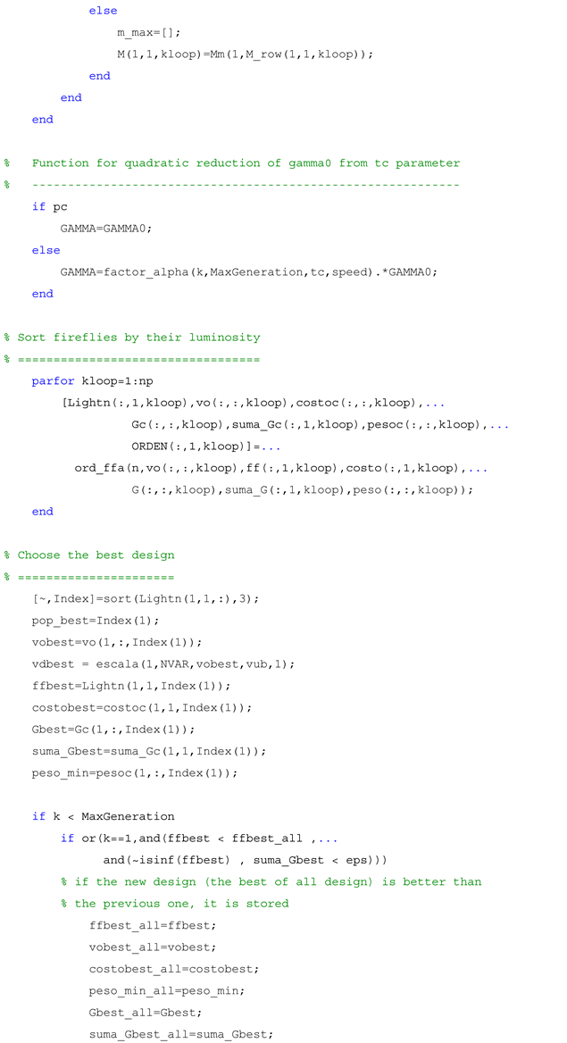
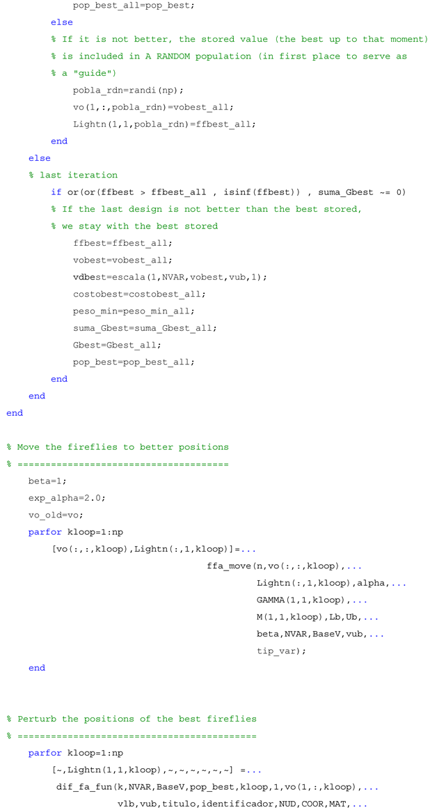
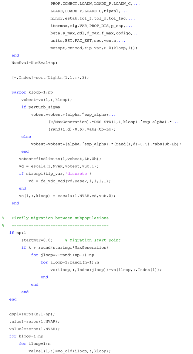
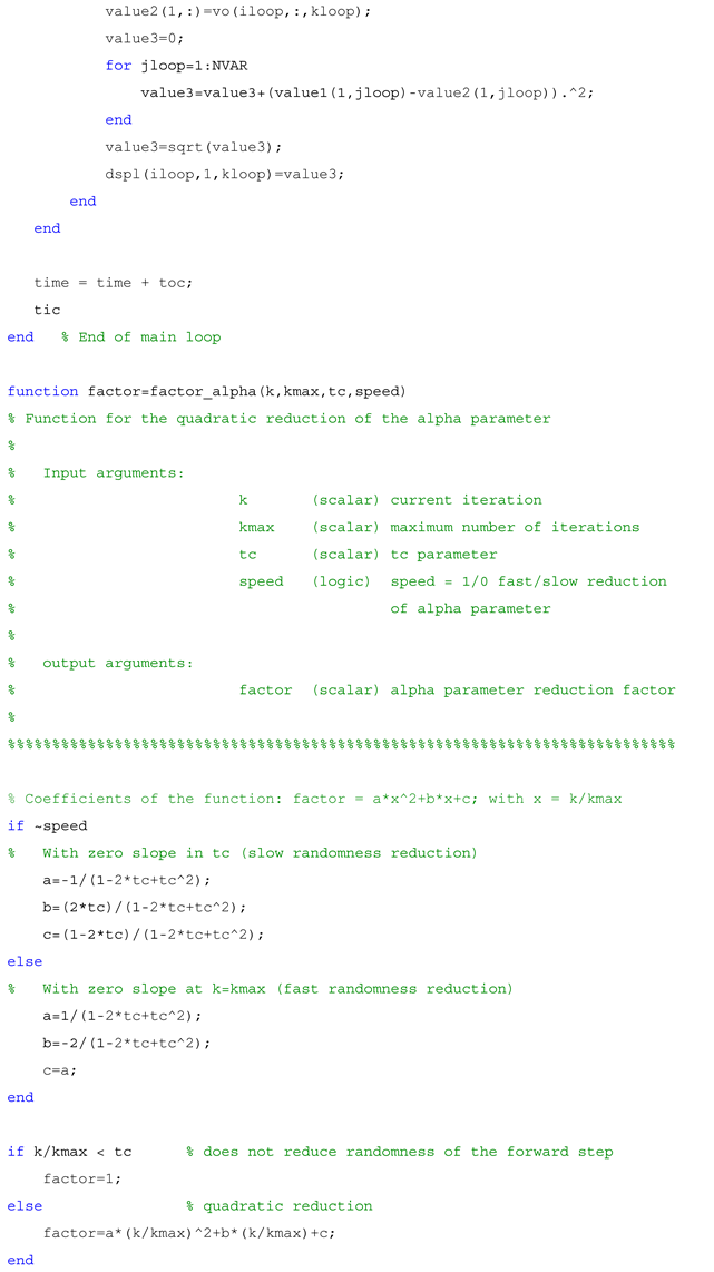
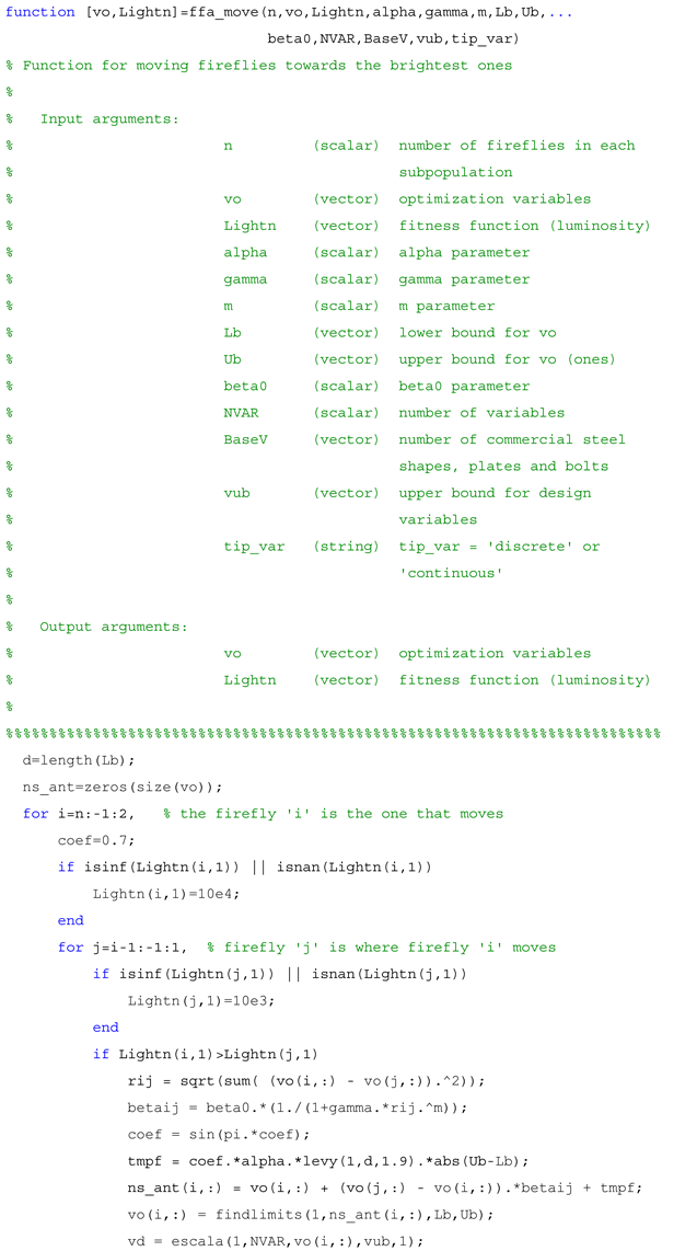
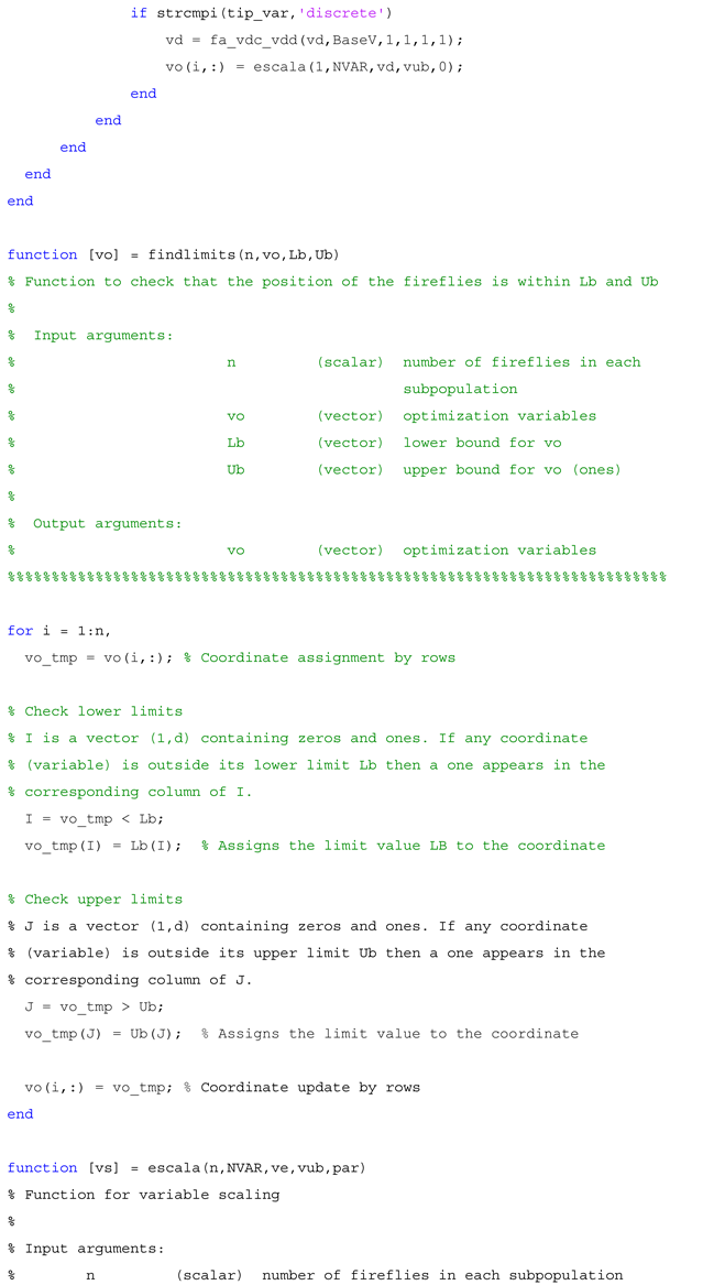
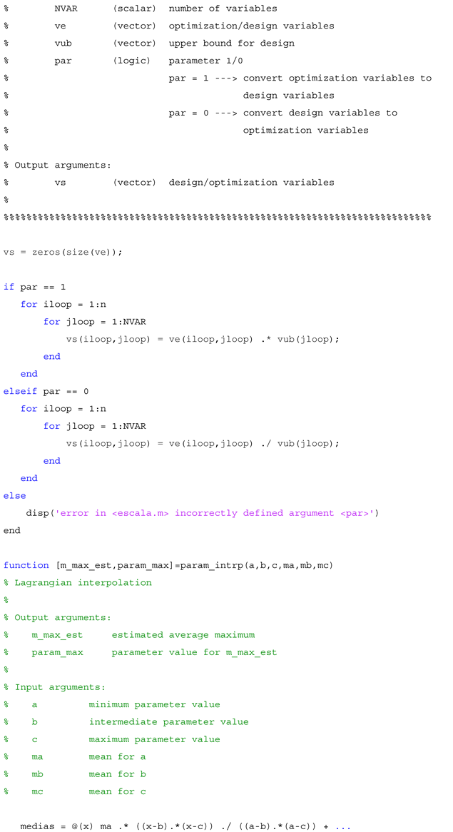
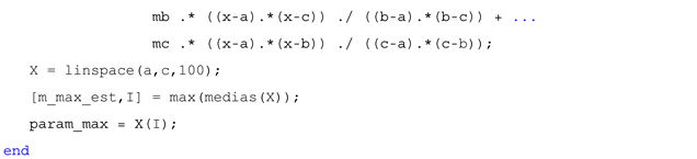
References
- Yang, X.-S. Nature-Inspired Optimization Algorithms, 2nd ed.; Elsevier: London, UK, 2021. [Google Scholar] [CrossRef]
- Wolpert, D.H.; Macready, W.G. No Free Lunch Theorems for Optimization. IEEE Trans. Evol. Comput. 1997, 1, 67–82. [Google Scholar] [CrossRef]
- Wolpert, D.H. Evolutionary computation and the processes of life: What the no free lunch theorems really mean: How to improve search algorithms. Ubiquity 2013, 2013, 1–15. [Google Scholar] [CrossRef]
- Joshi, S.K.; Bansal, J.C. Parameter tuning for meta-heuristics. Knowl.-Based Syst. 2020, 189, 105094. [Google Scholar] [CrossRef]
- Loubière, P.; Jourdan, A.; Siarry, P.; Chelouah, R. A sensitivity analysis method for driving the Artificial Bee Colony algorithm’s search process. Appl. Soft Comput. 2016, 41, 515–531. [Google Scholar] [CrossRef]
- Younis, M.T.; Yang, S. Hybrid meta-heuristic algorithms for independent job scheduling in grid computing. Appl. Soft Comput. 2018, 72, 498–517. [Google Scholar] [CrossRef]
- Yang, X.-S. Firefly Algorithms for Multimodal Optimization. In Stochastic Algorithms: Foundations and Applications, SAGA 2009; Watanabe, O., Zeugmann, T., Eds.; Lecture Notes in Computer, Sciences; Springer: Berlin/Heidelberg, Germany, 2009; Volume 5792, pp. 169–178. [Google Scholar] [CrossRef]
- Fister, I.; Fister, I., Jr.; Yang, X.S.; Brest, J. A comprehensive review of firefly algorithms. Swarm Evol. Comput. 2013, 13, 34–46. [Google Scholar] [CrossRef]
- Yang, X.-S. Cuckoo Search and Firefly Algorithm: Overview and Analysis. In Cuckoo Search and Firefly Algorithm. Theory and Applications, 1st ed.; Yang, X.-S., Ed.; Studies in Computational Intelligence; Springer: Cham, Swizerland, 2014; Volume 516, pp. 1–26. [Google Scholar] [CrossRef]
- Leite, J.P.B.; Topping, B.H.V. Parallel simulated annealing for structural optimization. Comput. Struct. 1999, 73, 545–564. [Google Scholar] [CrossRef]
- Thierauf, G.; Cai, J. Parallel evolution strategy for solving structural optimization. Eng. Struct. 1997, 19, 318–324. [Google Scholar] [CrossRef]
- Gomes, G.M.; Esposito, A. A Parallelised Firefly Algorithm for Structural Size and Shape Optimization with Multimodal Constraints. In Cuckoo Search and Firefly Algorithm. Theory and Applications, 1st ed.; Yang, X.-S., Ed.; Studies in Computational Intelligence; Springer: Cham, Swizerland, 2014; Volume 516, pp. 291–314. [Google Scholar] [CrossRef]
- Hasanҫebi, O.; Bahҫecioǧlu, T.; Kurҫ, Ö.; Saka, M.P. Optimum design of high-rise steel buildings using an evolution strategy integrated parallel algorithm. Comput. Struct. 2011, 89, 2037–2051. [Google Scholar] [CrossRef]
- Truong, V.H.; Nguyen, P.C.; Kim, S.E. An efficient method for optimizing space steel frames with semi-rigid joints using practical advanced analysis and the micro-genetic algorithm. J. Constr. Steel Res. 2017, 128, 416–427. [Google Scholar] [CrossRef]
- Huang, H.C. FPGA-Based Parallel Metaheuristic PSO Algorithm and Its Application to Global Path Planning for Autonomous Robot Navigation. J. Intell. Robot. Syst. 2014, 76, 475488. [Google Scholar] [CrossRef]
- Soria-Alcaraz, A.J.; Carpio, M.; Puga, H.; Swan, J.; Melin, P.; Terashima, H.; Sotelo-Figueroa, A.M. Parallel Meta-heuristic Approaches to the Course Timetabling Problem. In Design of Intelligent Systems Based on Fuzzy Logic, Neural Networks and Nature-Inspired Optimization; Melin, P., Castillo, O., Kacprzyk, J., Eds.; Studies in Computational Intelligence; Springer: Cham, Swizerland, 2015; Volume 601, pp. 391–417. [Google Scholar] [CrossRef]
- Wang, C.H.; Nguyen, T.T.; Pan, J.S.; Dao, T.K. An Optimization Approach for Potential Power Generator Outputs Based on Parallelized Firefly Algorithm. In Advances in Intelligent Information Hiding and Multimedia Signal Processing, Smart Innovation, Systems and Technologies; Pan, J.S., Tsai, P.W., Huang, H.C., Eds.; Springer: Cham, Swizerland, 2017; Volume 64, pp. 297–306. [Google Scholar] [CrossRef]
- Gandomi, A.H.; Yang, X.-S.; Alavi, A.H. Mixed variable structural optimization using Firefly Algorithm. Comput. Struct. 2011, 89, 2325–2336. [Google Scholar] [CrossRef]
- Talatahari, S.; Gandomi, A.H.; Yun, G.J. Optimum design of tower structures using Firefly Algorithm. Struct. Des. Tall Spec. Build. 2012, 23, 350–361. [Google Scholar] [CrossRef]
- Talbi, E. Metaheuristics: From Design to Implementation; John Wiley & Sons: Hoboken, NJ, USA, 2009. [Google Scholar]
- Sánchez-Olivares, G.; Tomás, A. Design of planar semi-rigid Steel frames using genetic algorithms and Component Method. J. Constr. Steel Res. 2013, 88, 267–278. [Google Scholar] [CrossRef]
- Eiben, A.E.; Smit, S.K. Parameter tuning for configuring and analyzing evolutionary algorithms. Swarm Evol. Comput. 2011, 1, 19–31. [Google Scholar] [CrossRef]
- Sánchez-Olivares, G.; Tomás, A. Optimization of Reinforced Concrete Sections under Compression and Biaxial Bending by Using a Parallel Firefly Algorithm. Appl. Sci. 2021, 11, 2076. [Google Scholar] [CrossRef]
- EN 1993-1-1:2005; Eurocode 3 Design of Steel Structures—Part 1—1: General Rules and Rules for Buildings. European Committee for Standardisation (CEN): Brussels, Belgium, 2005.
- Sánchez-Olivares, G.; Tomás, A. Improvements in meta-heuristic algorithms for minimum cost design of reinforced concrete rectangular sections under compression and biaxial bending. Eng. Struct. 2017, 130, 162–179. [Google Scholar] [CrossRef]
- Yang, X.-S.; Deb, S. Multiobjective cuckoo search for design optimization. Comput. Oper. Res. 2013, 40, 1616–1624. [Google Scholar] [CrossRef]
- Gandomi, A.H.; Yang, X.-S.; Talatahari, S.; Alavi, A.H. Firefly algorithm with chaos. Commun. Nonlinear Sci. Numer. Simul. 2013, 18, 89–98. [Google Scholar] [CrossRef]
- De Jong, K. Parameter Setting in EAs: A 30 Year Perspective. In Parameter Setting in Evolutionary Algorithms. Studies in Computational Intelligence; Lobo, F.G., Lima, C.F., Michalewicz, Z., Eds.; Springer: Berlin/Heidelberg, Germany, 2007; Volume 54, pp. 1–18. [Google Scholar] [CrossRef]
- Gandomi, A.H.; Kashani, A.R.; Roke, D.A.; Mousavi, M. Optimization of retaining wall design using recent swarm intelligence techniques. Eng. Struct. 2015, 103, 72–84. [Google Scholar] [CrossRef]
- Morris, M.D. Factorial sampling plans for preliminary computational experiments. Technometrics 1991, 33, 161–174. [Google Scholar] [CrossRef]
- Liang, J.; Qu, B.; Suganthan, P.; Chen, Q. Problem Definitions and Evaluation Criteria for the Cec 2015 Competition on Learning-Based Real-Parameter Single Objective Optimization; Technical Report201411A, Computational Intelligence Laboratory, Zhengzhou University, Zhengzhou China and Technical Report; Nanyang Technological University: Singapore, 2015. [Google Scholar]
- Cabrero, J.M.; Bayo, E. Development of practical design methods for steel structures with semi-rigid connections. Eng. Struct. 2005, 27, 1125–1137. [Google Scholar] [CrossRef]
- Ali, N.B.H.; Sellami, M.; Cutting-Decelle, A.F.; Mangin, J.C. Multi-stage production cost optimization of semi-rigid steel frames using genetic algorithms. Eng. Struct. 2009, 31, 2766–2778. [Google Scholar] [CrossRef]
- Xu, L.; Grierson, D.E. Computer-automated design of semirigid steel frameworks. J. Struct. Eng. 1993, 119, 1740–1760. [Google Scholar] [CrossRef]
- Foley, C.M.; Schinler, D. Automated design of steel frames using advanced analysis and object-oriented evolutionary computation. J. Struct. Eng. 2003, 129, 648–660. [Google Scholar] [CrossRef]
- Kameshki, E.S.; Saka, M.P. Genetic algorithm based optimum design of nonlinear planar steel frames with various semi-rigid connections. J. Constr. Steel Res. 2003, 59, 109–134. [Google Scholar] [CrossRef]
- Benavides, E.M. Information, entropy and its relationship to design. In Advanced Engineering Design. An Integrated Approach; Benavides, E.M., Ed.; Woodhead Publishing: Cambridge, UK, 2012; pp. 41–258. [Google Scholar] [CrossRef]
- Harte, J.; Newman, E.A. Maximum information entropy: A foundation for ecological theory. Trends Ecol. Evol. 2014, 29, 384–389. [Google Scholar] [CrossRef]
- Souza de Cursi, E.; Sampaio, R. Maximum Entropy and Information. In Uncertainty Quantification and Stochastic Modeling with Matlab; Souza de Cursi, E., Sampaio, R., Eds.; Elsevier: London, UK, 2015; pp. 133–175. [Google Scholar] [CrossRef]
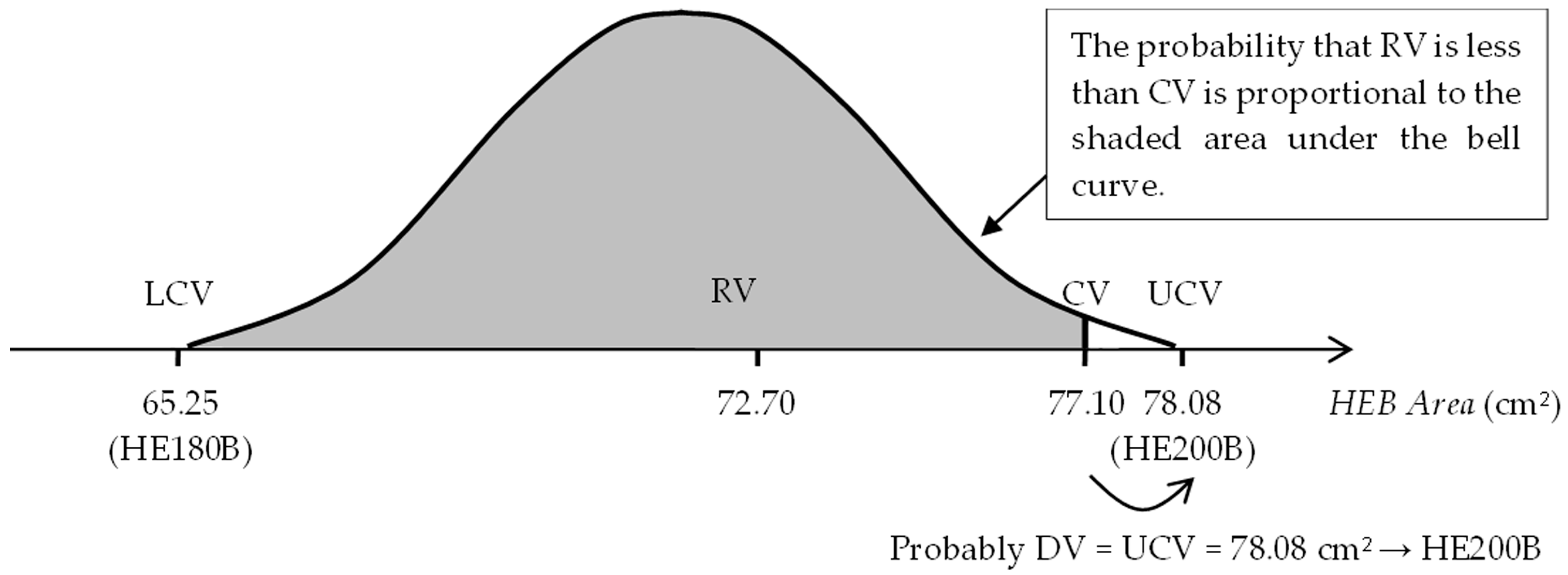
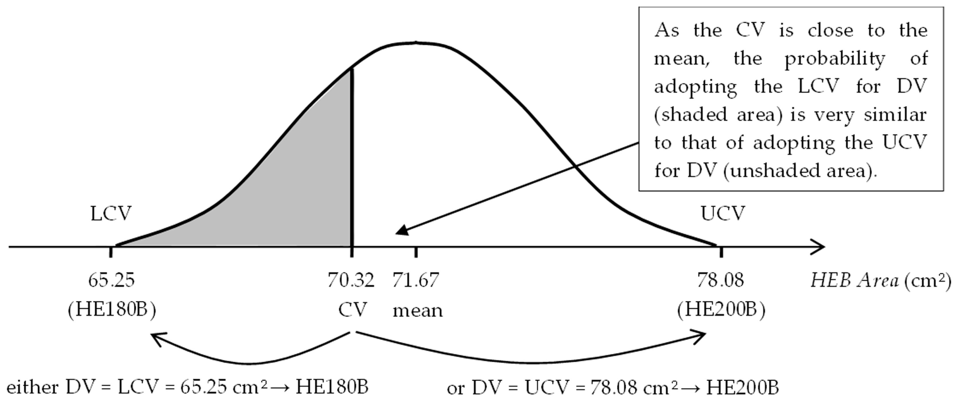
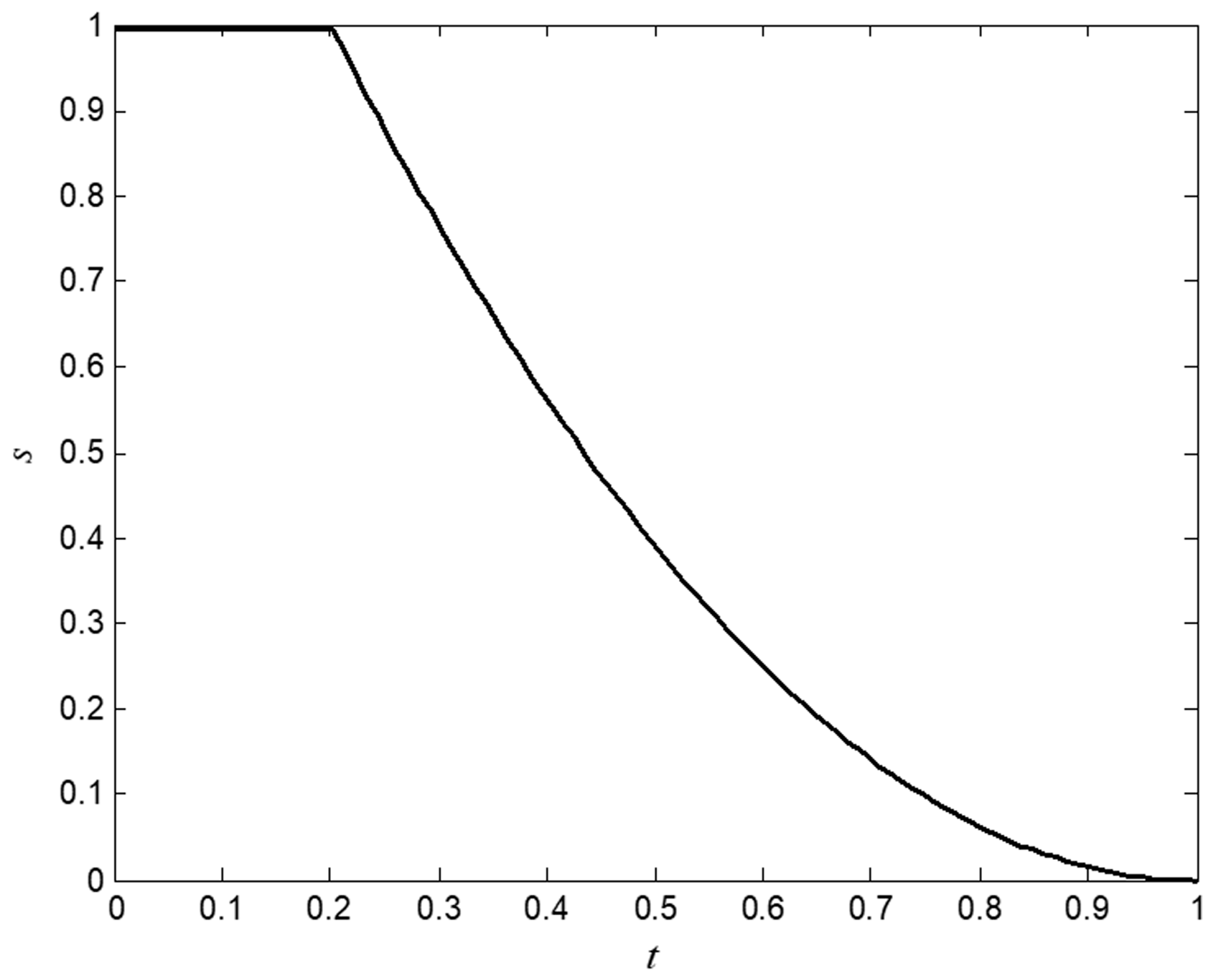
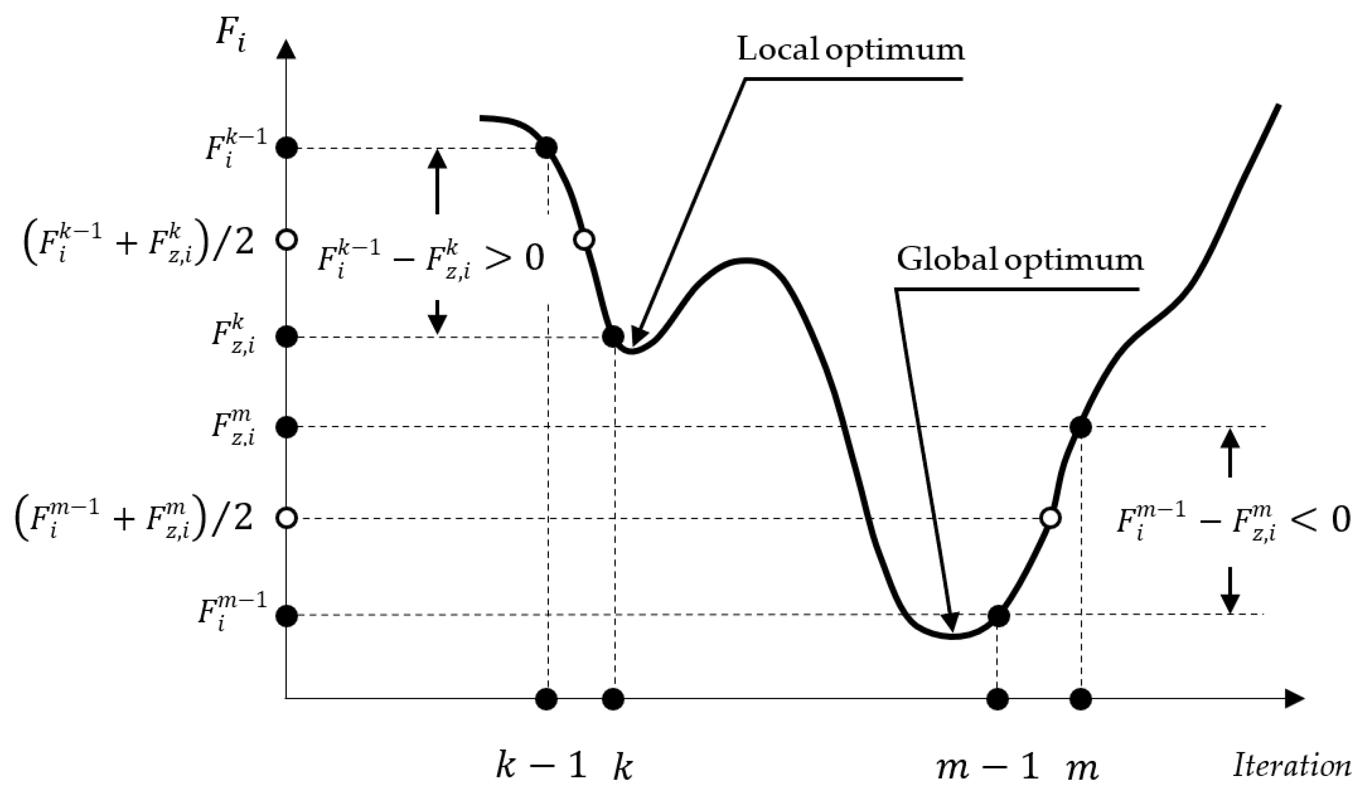
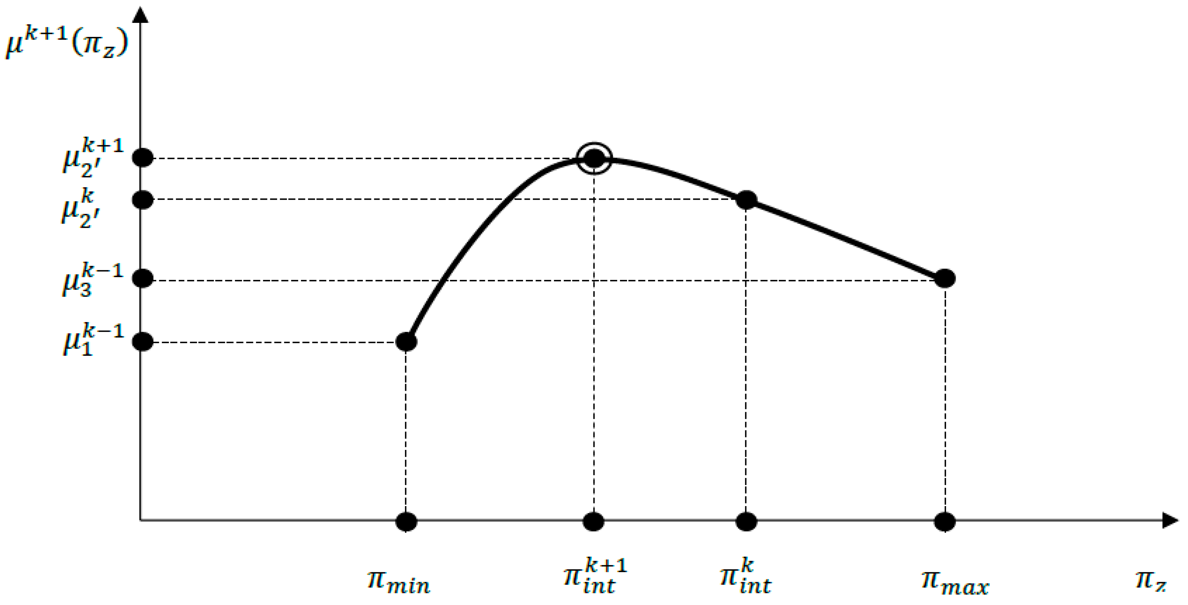
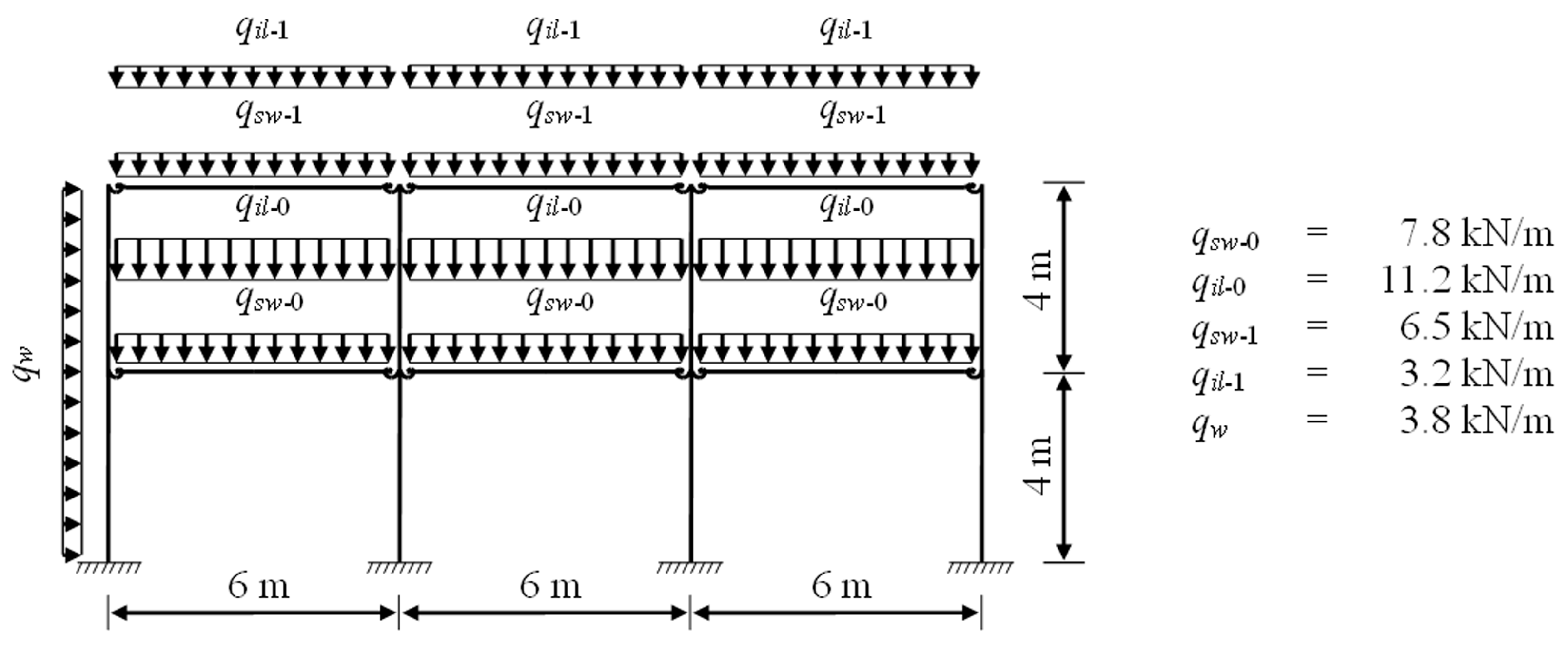
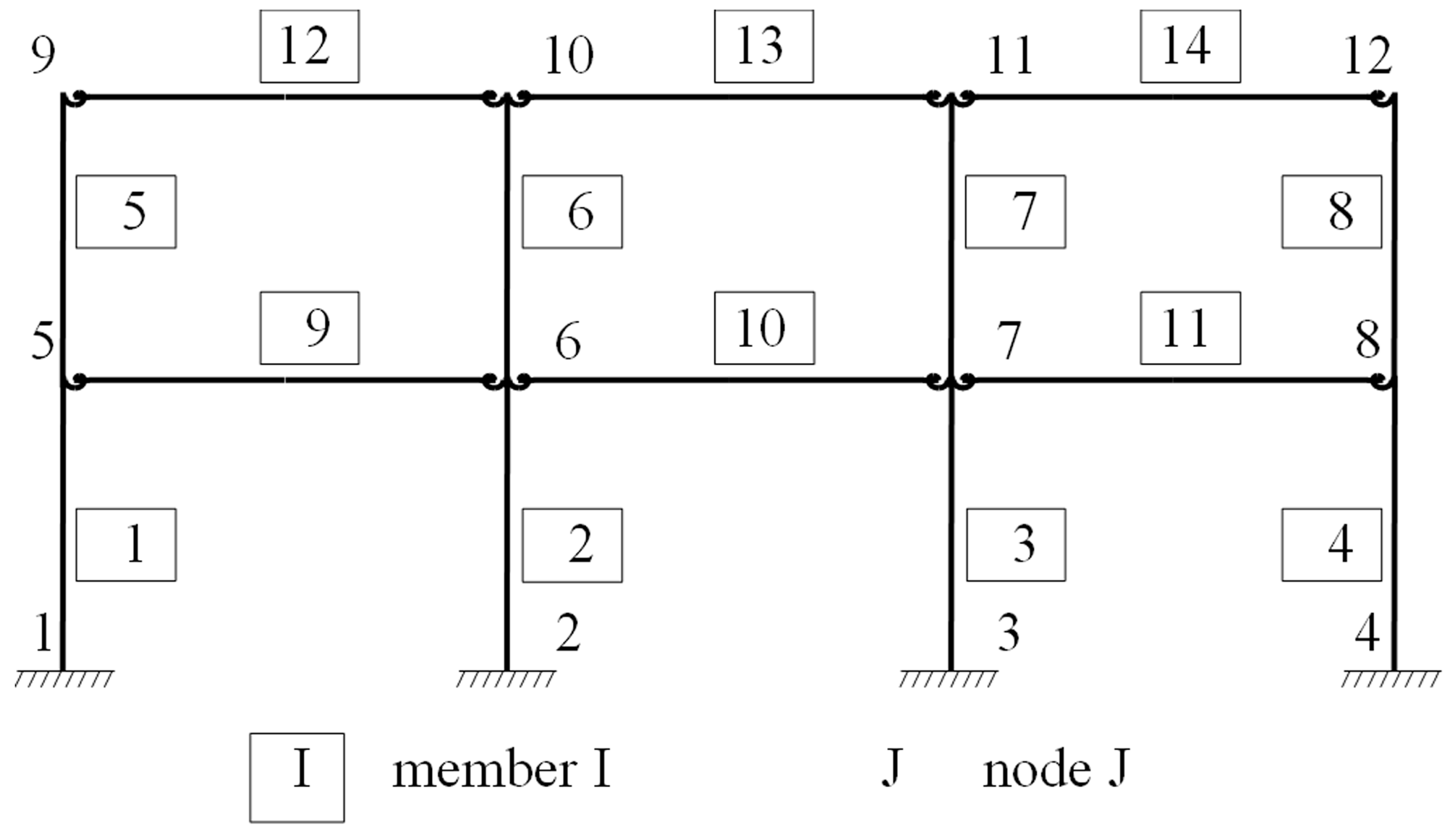
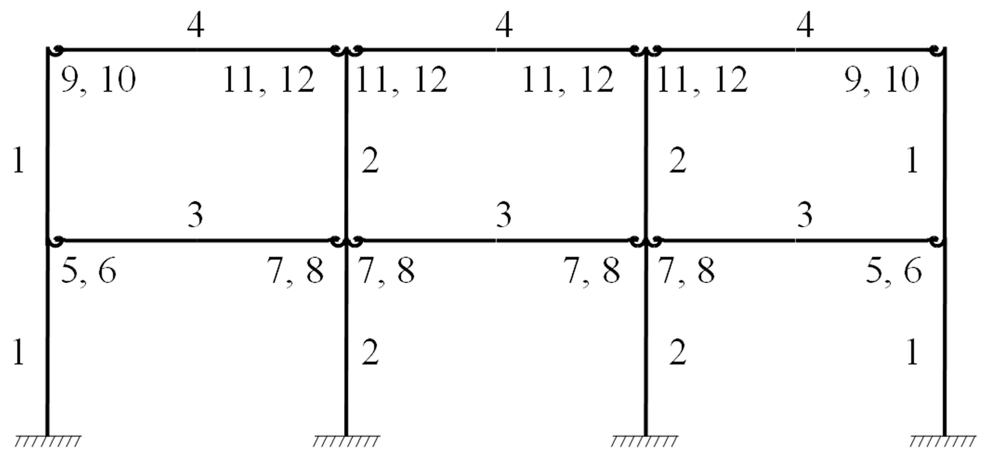
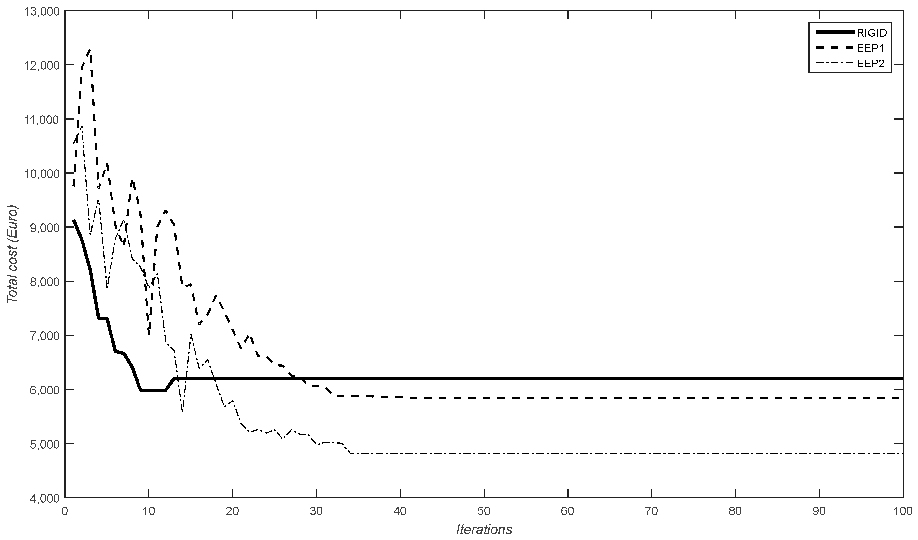
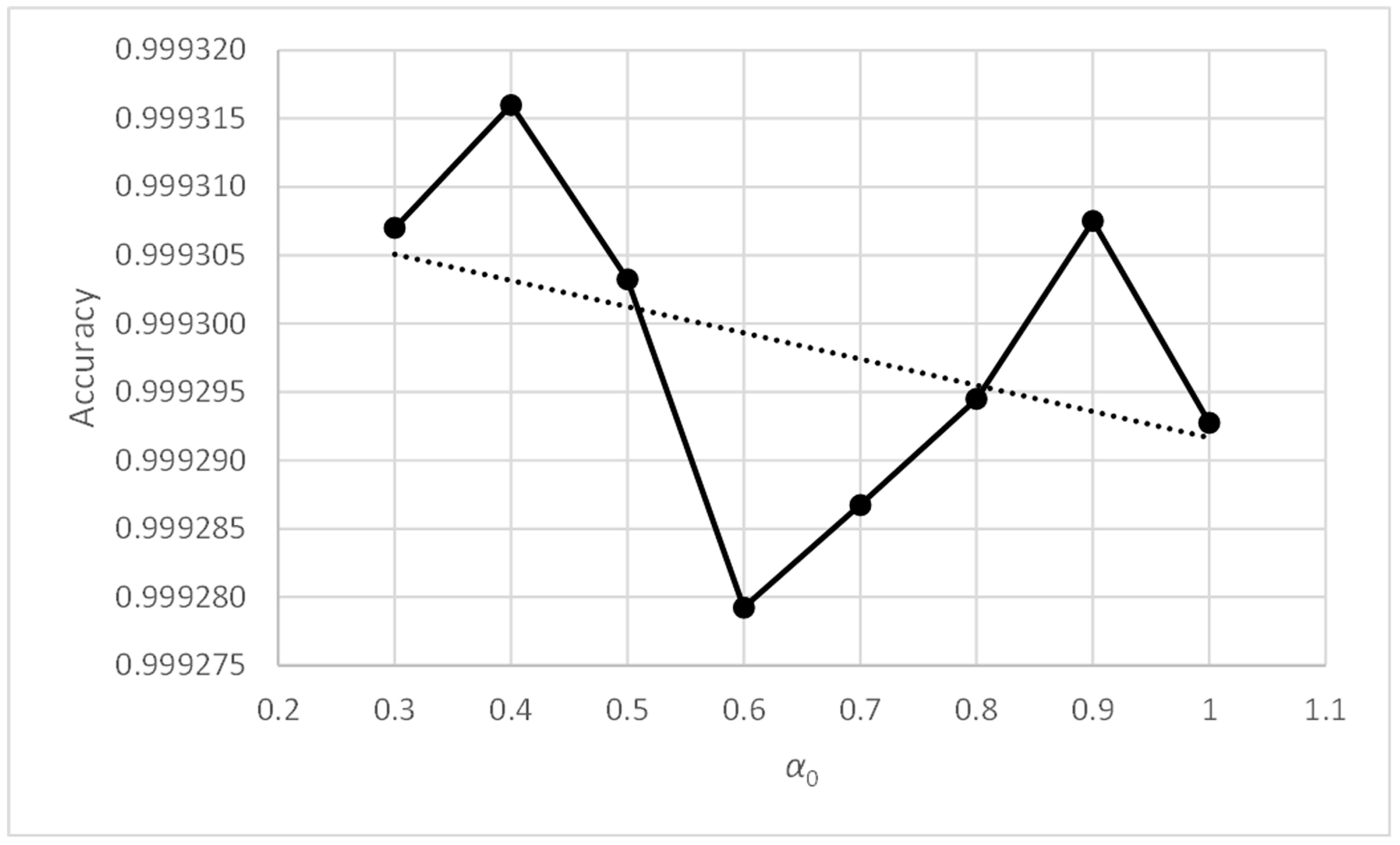
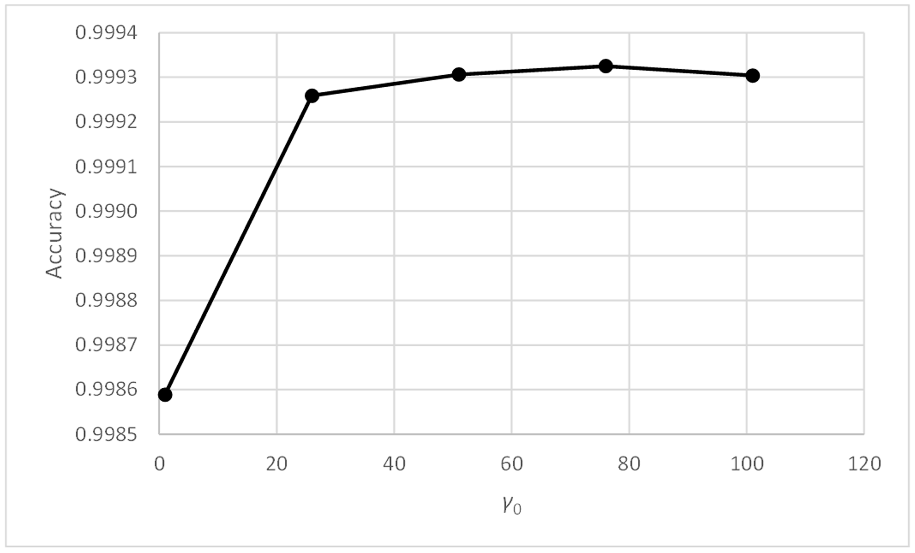
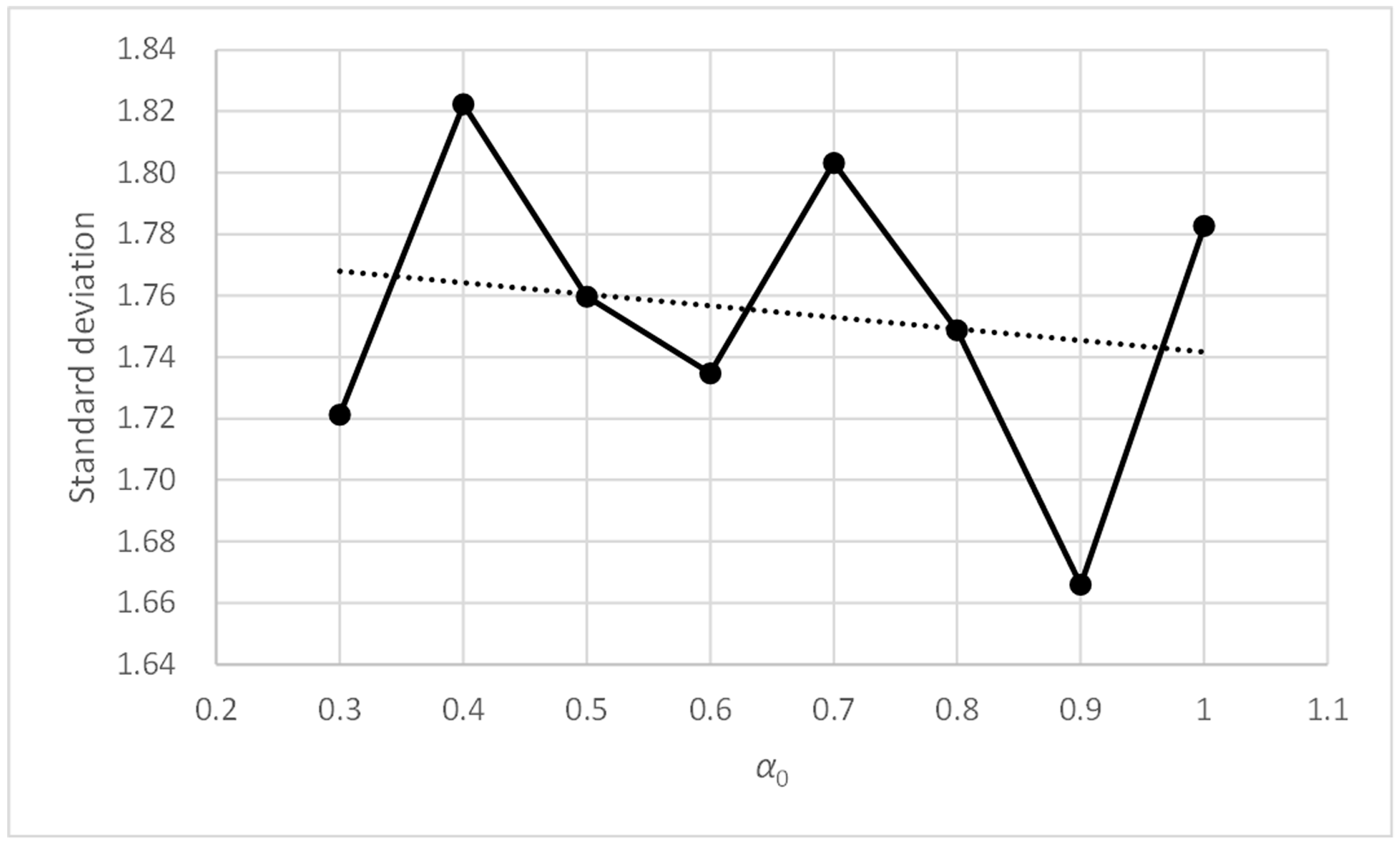

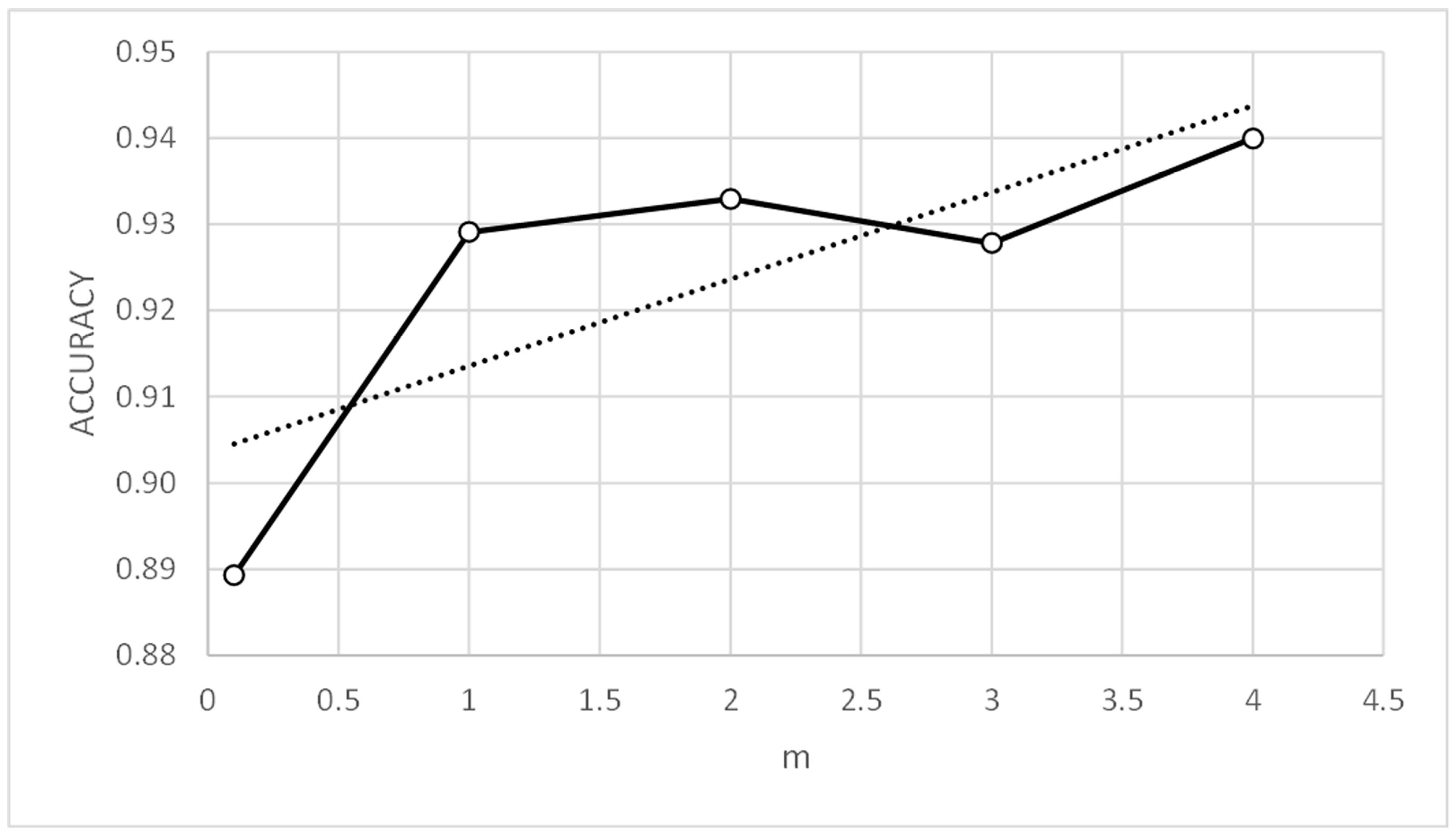
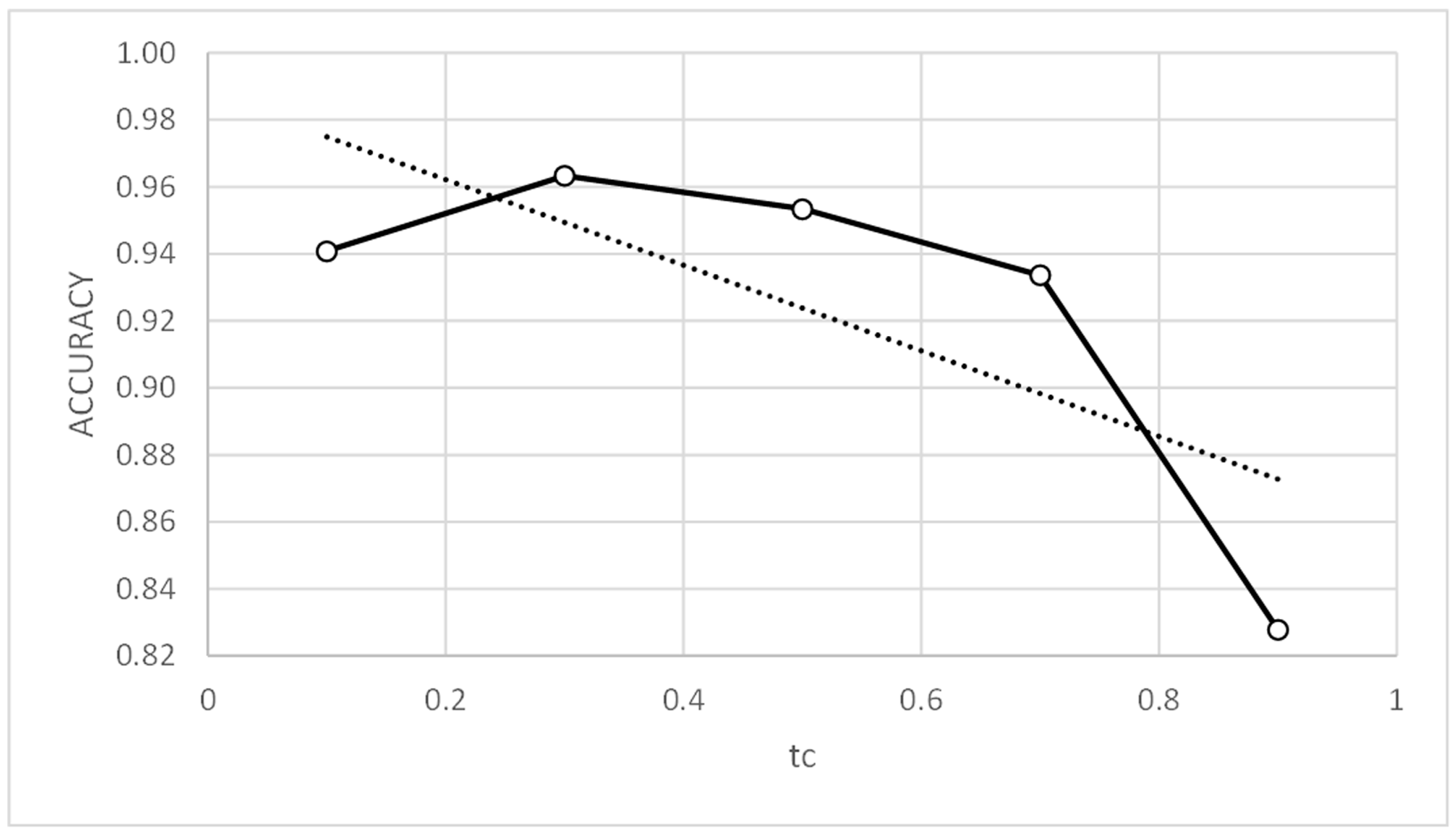


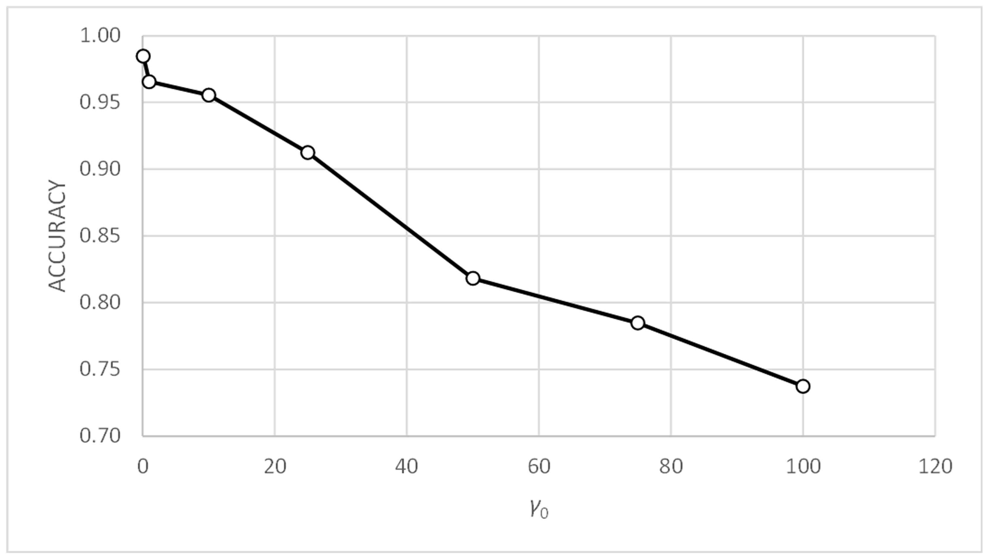
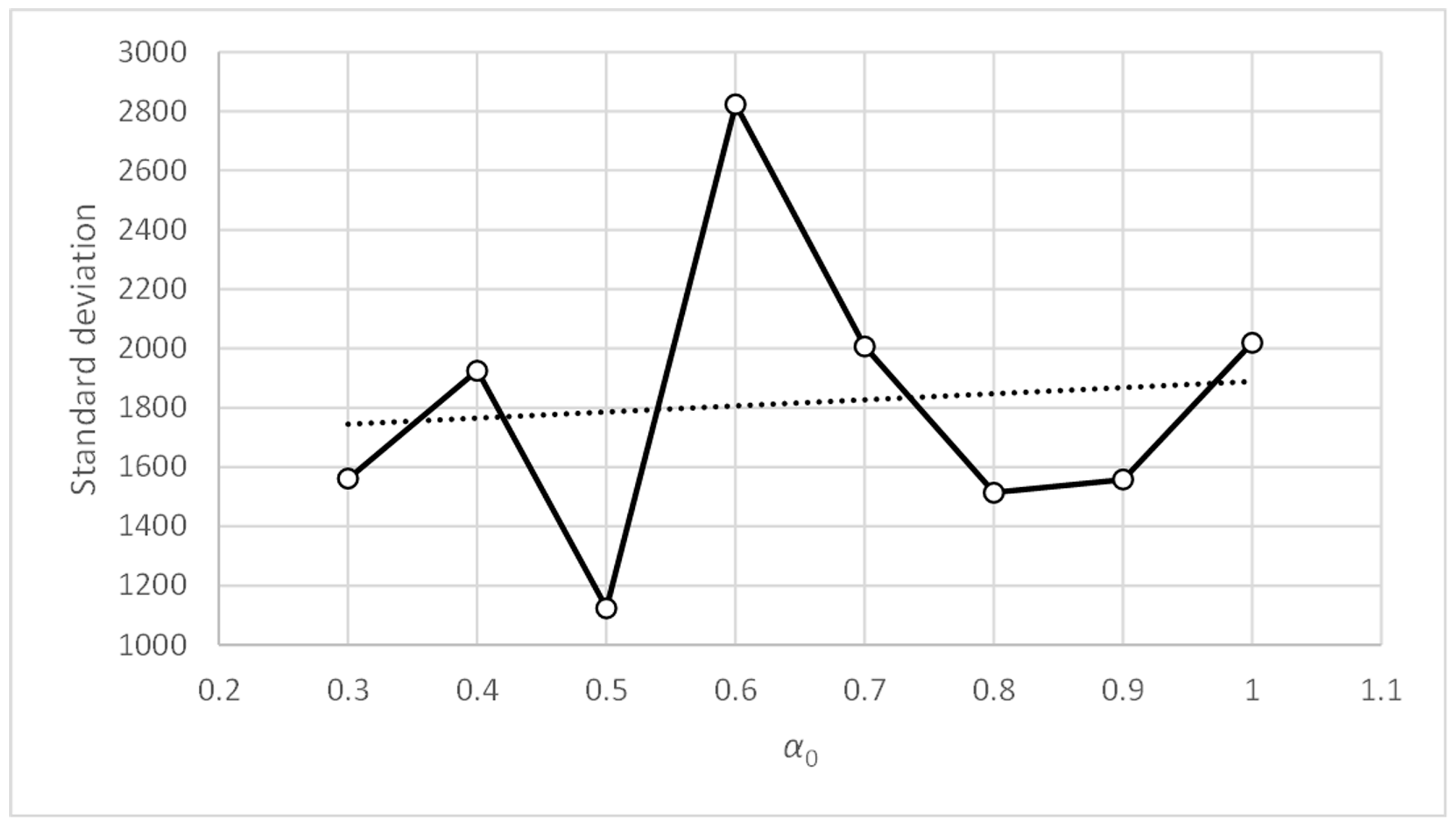
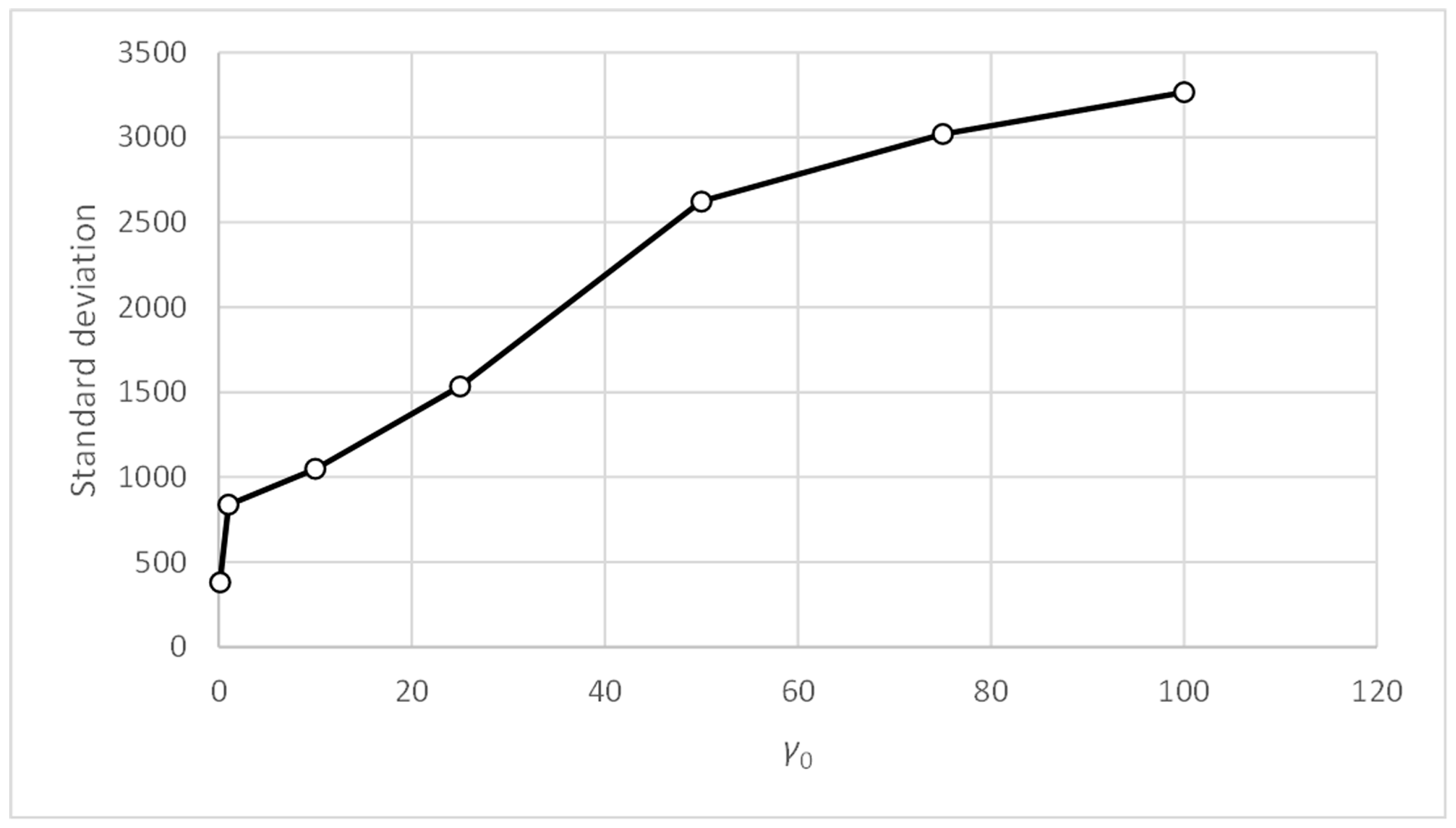
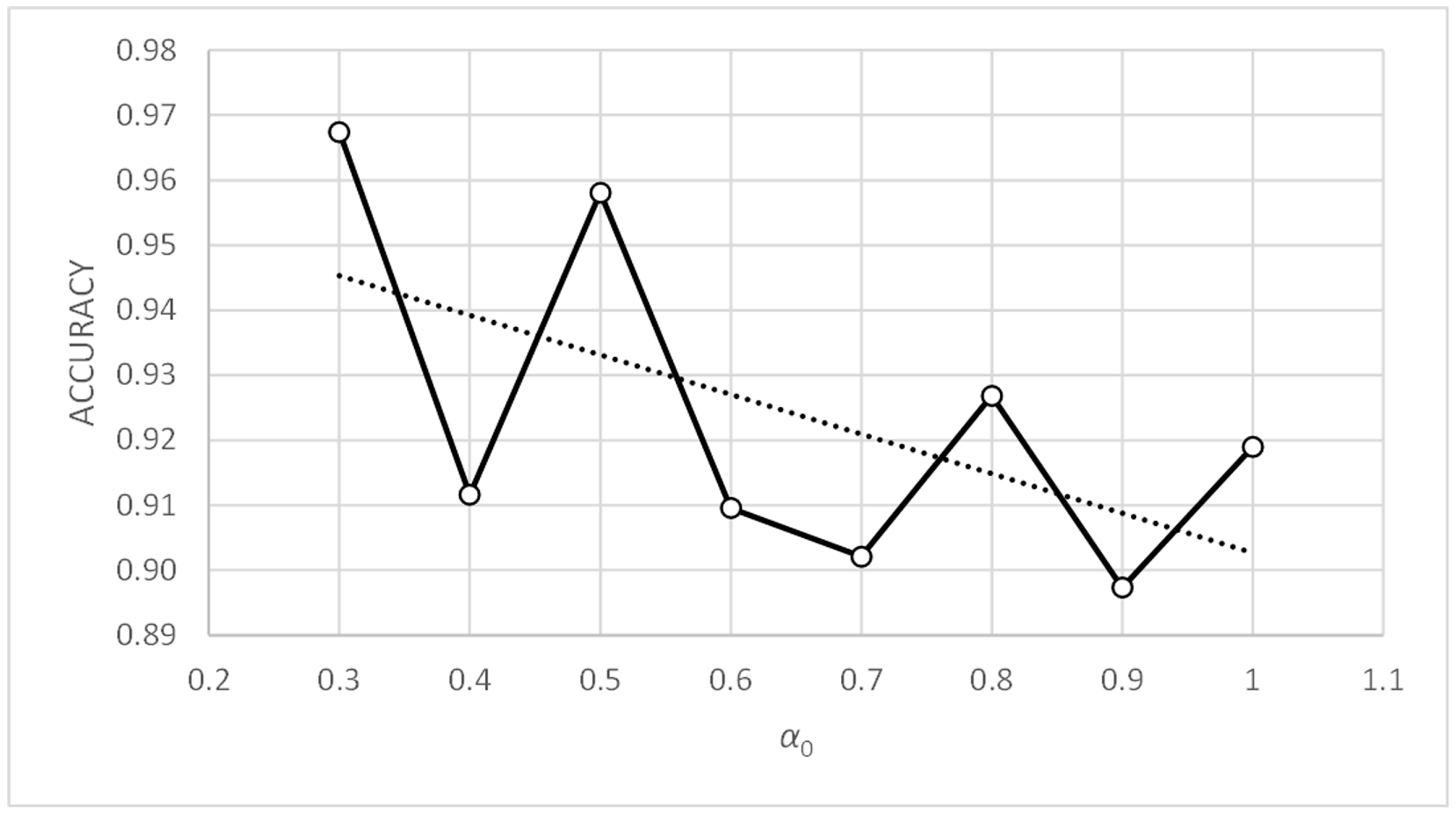
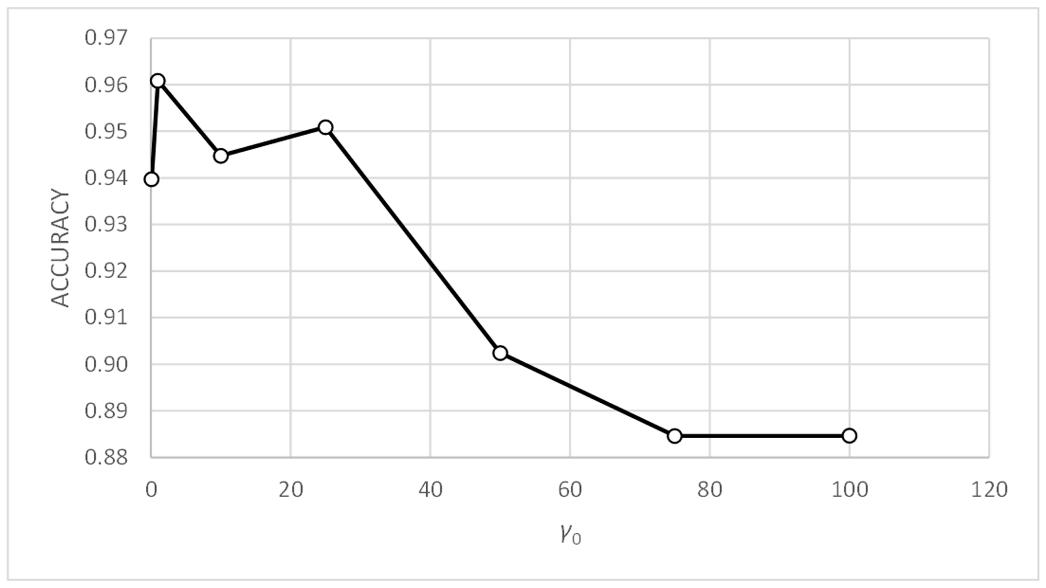
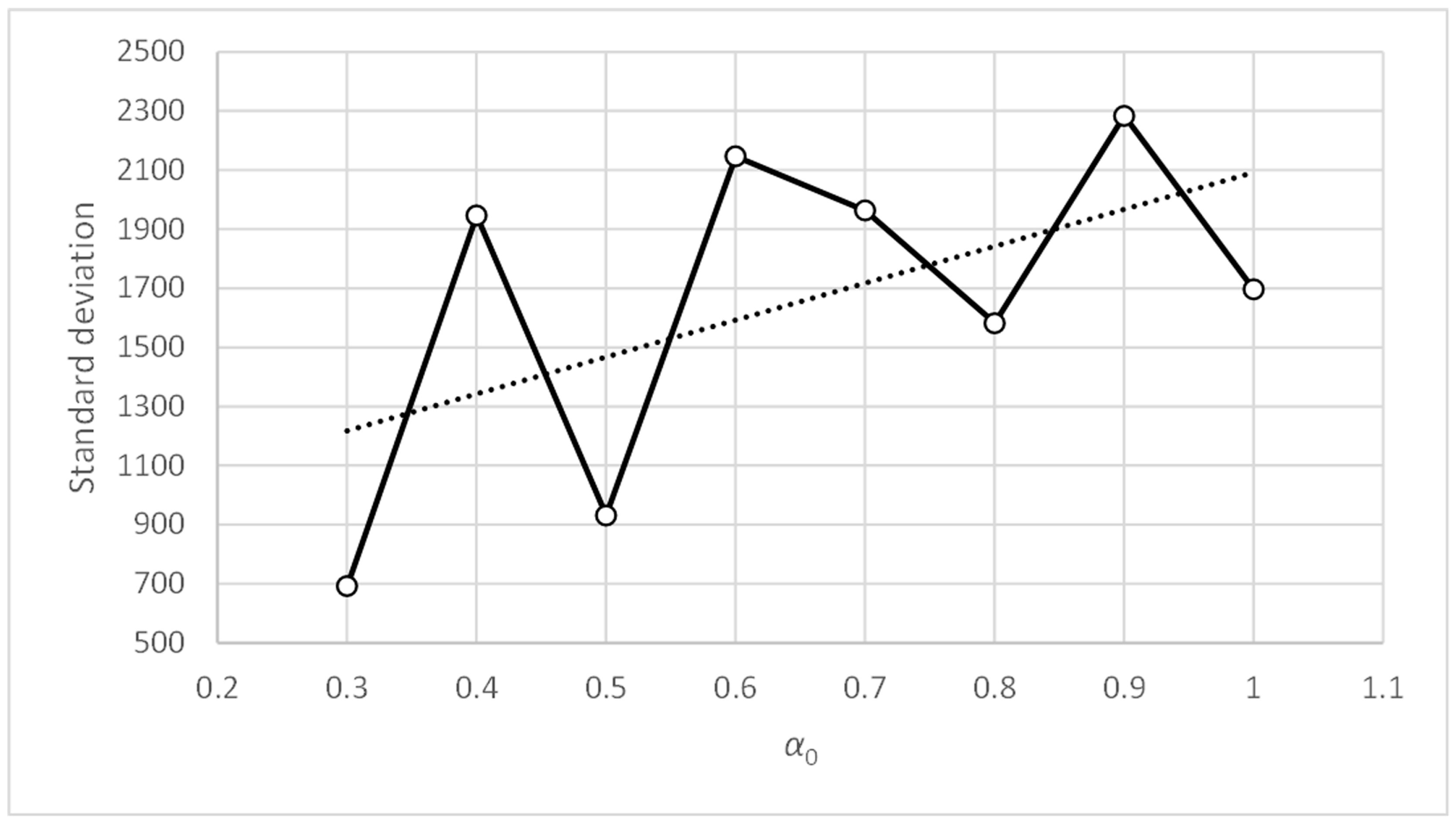
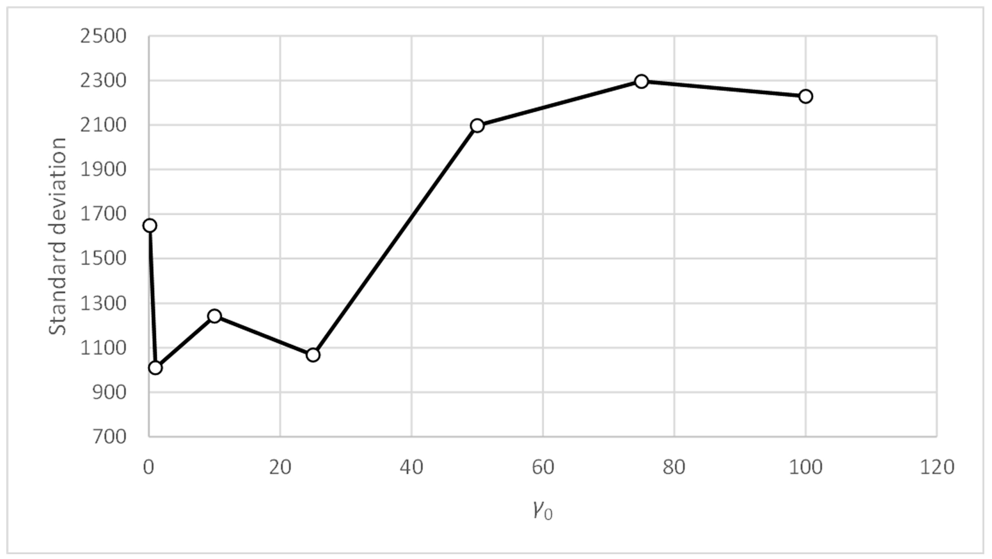
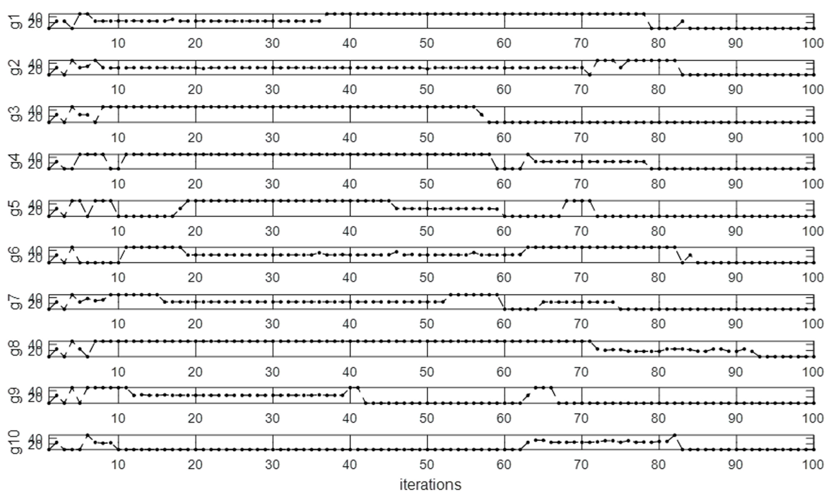
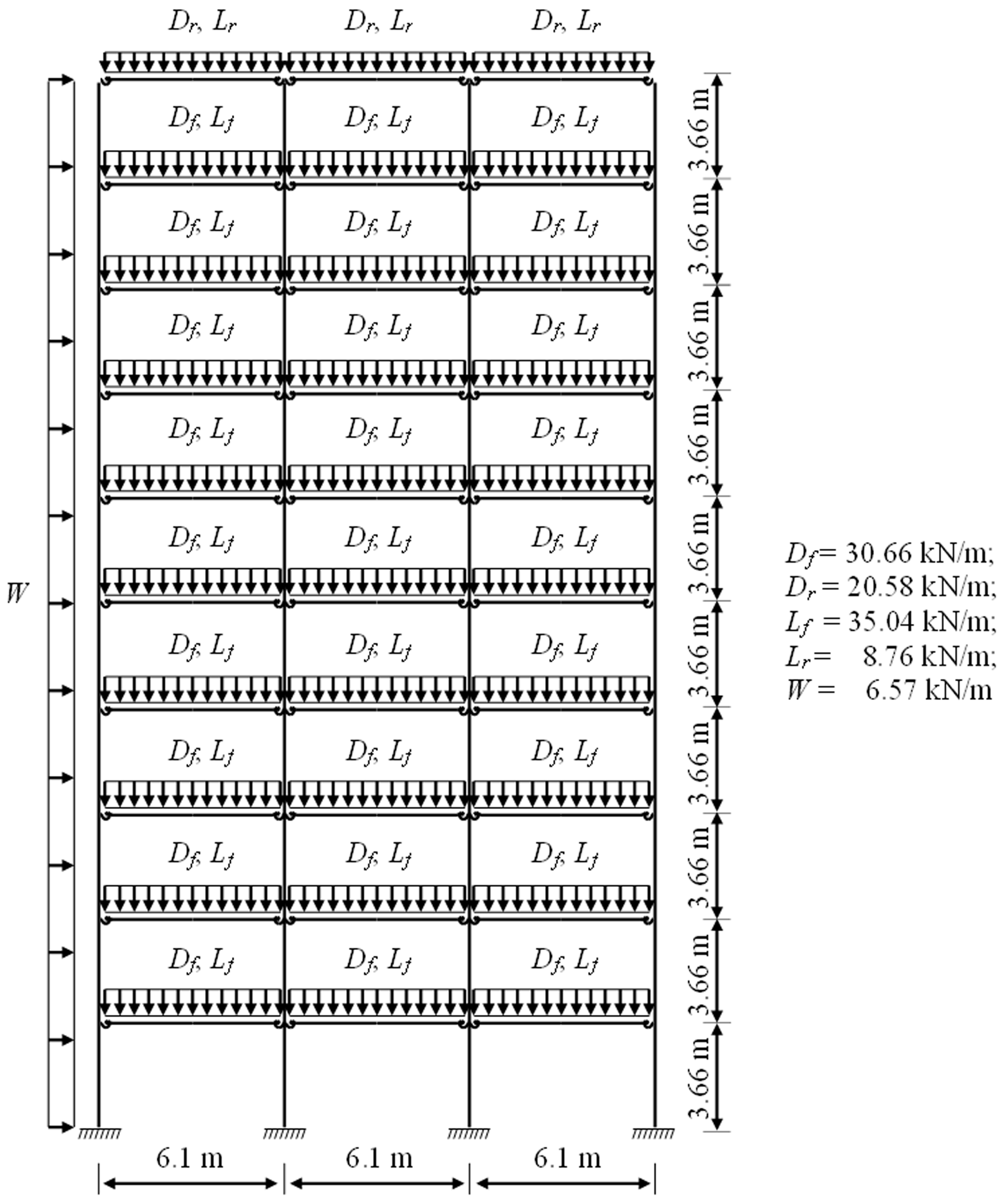
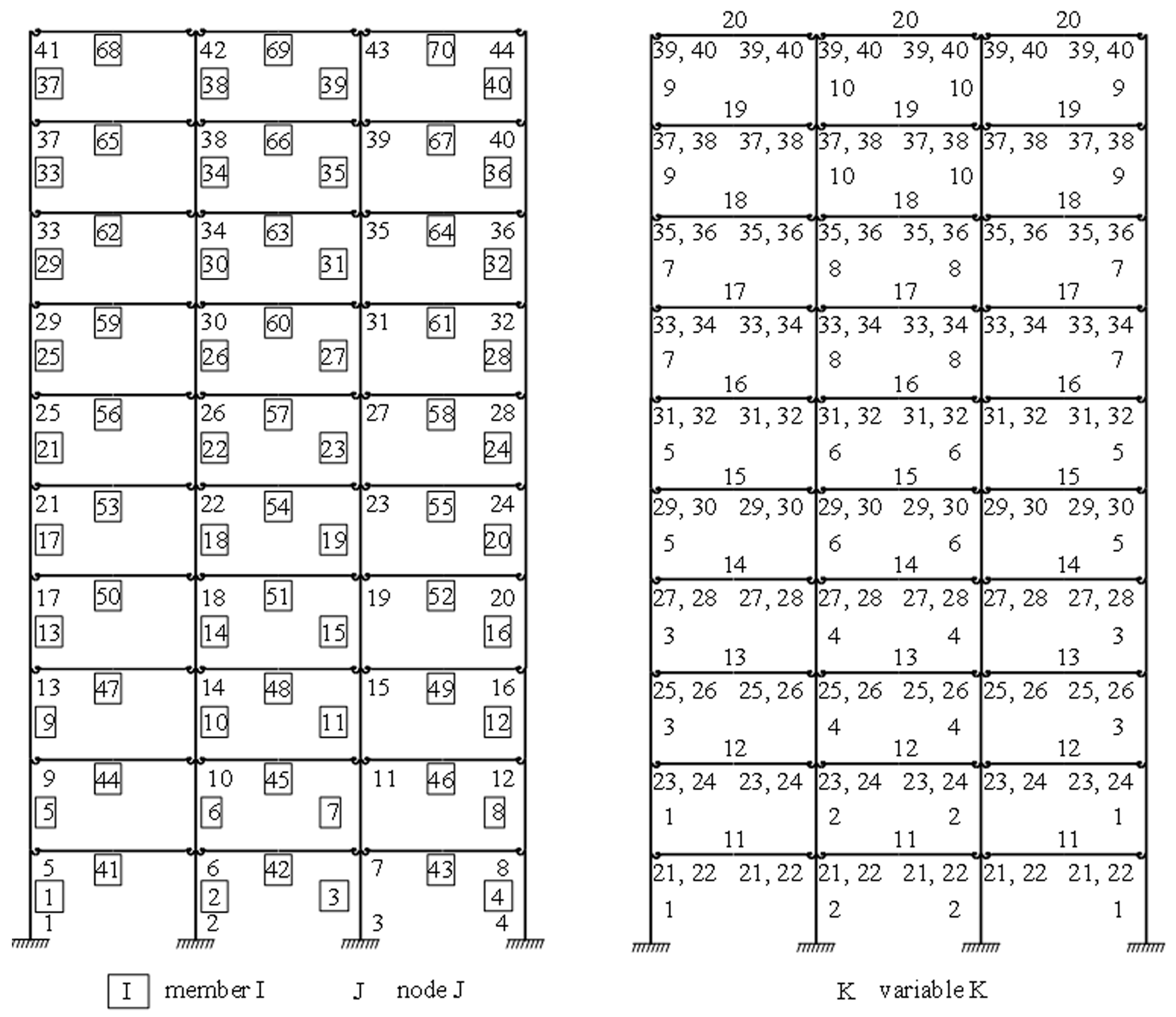
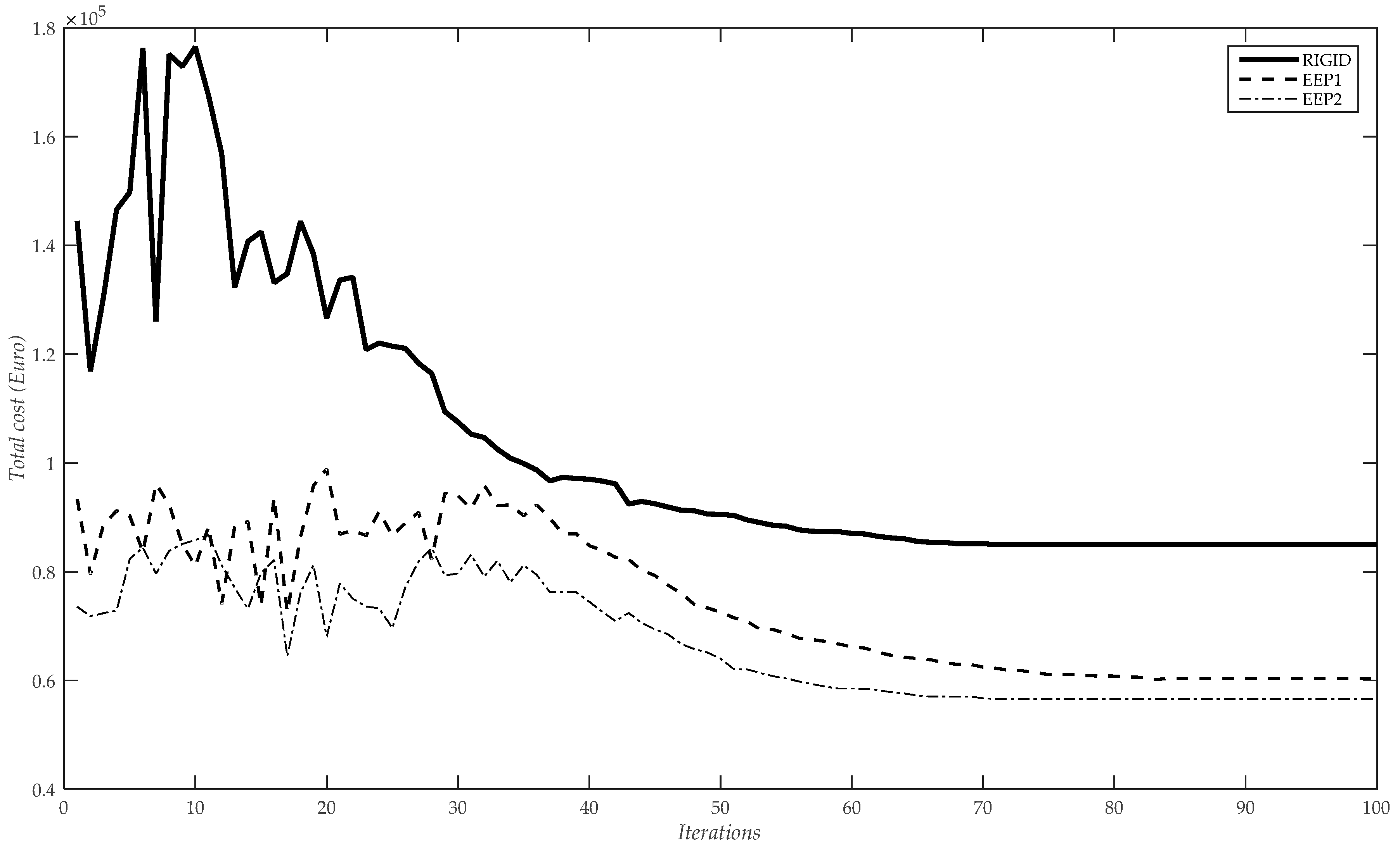

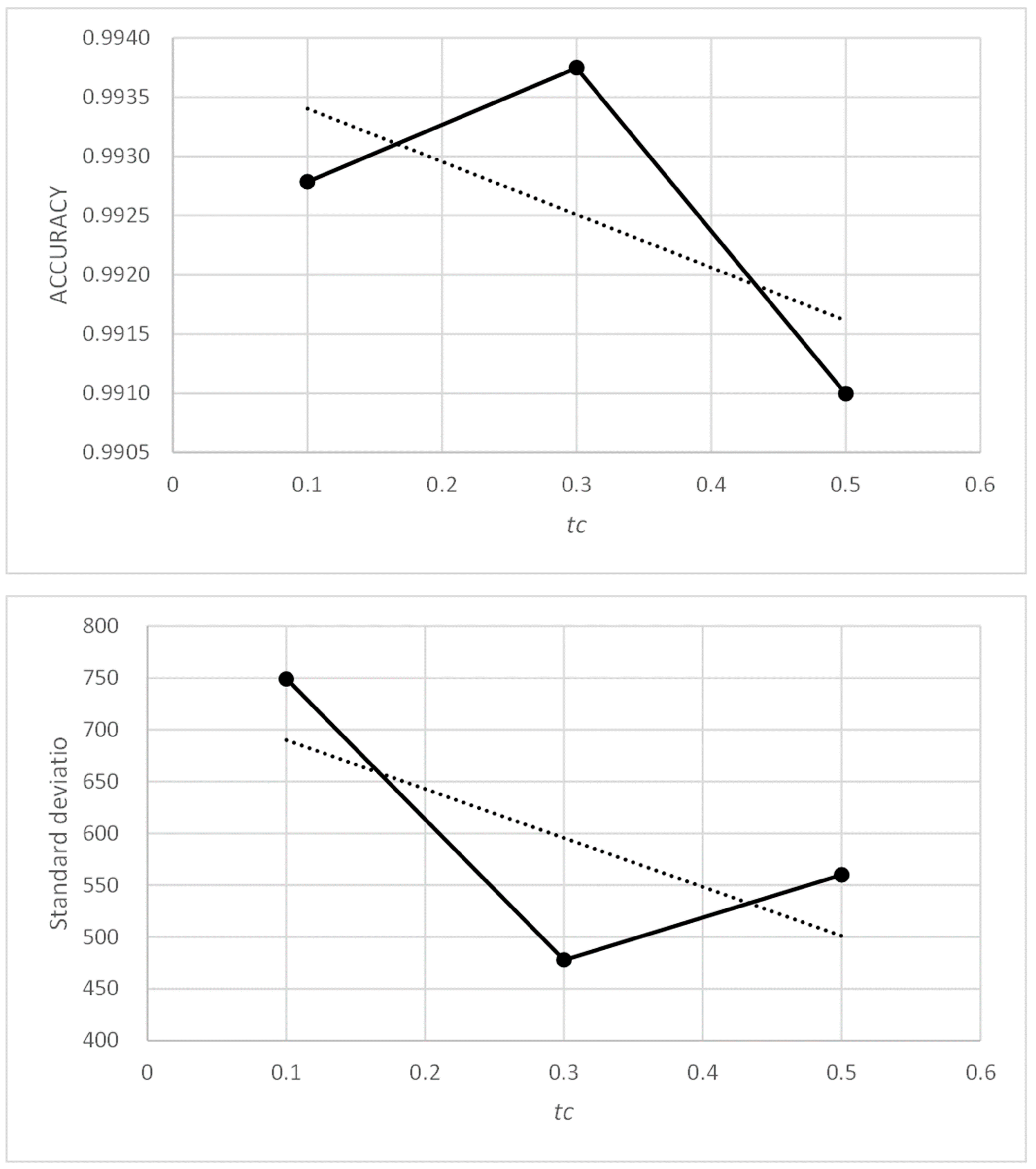
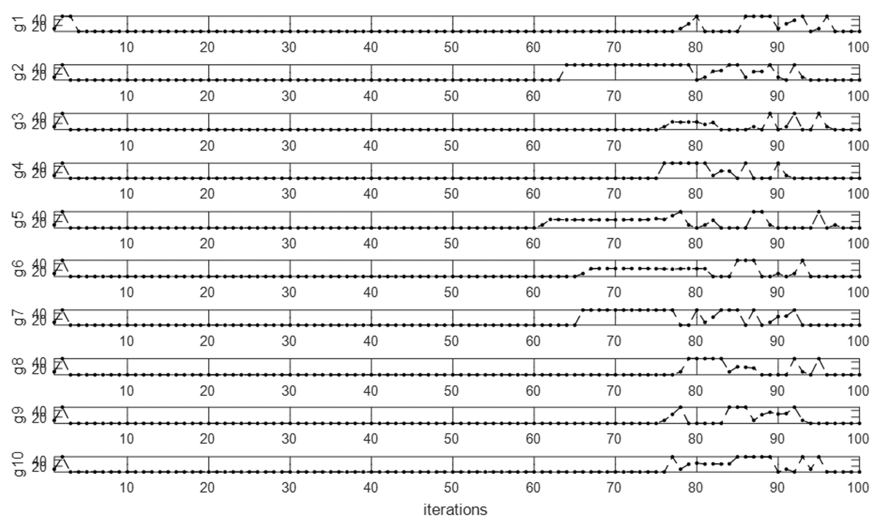
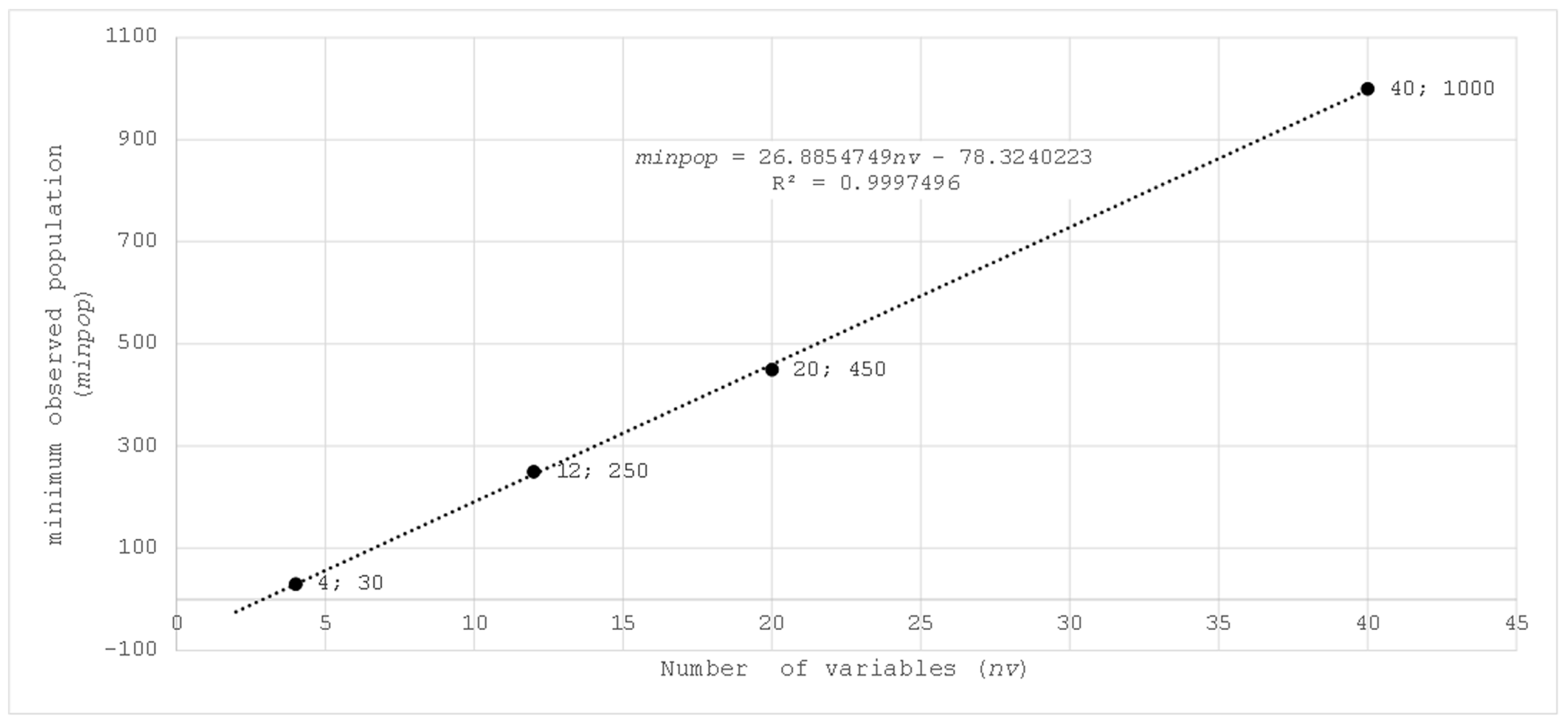
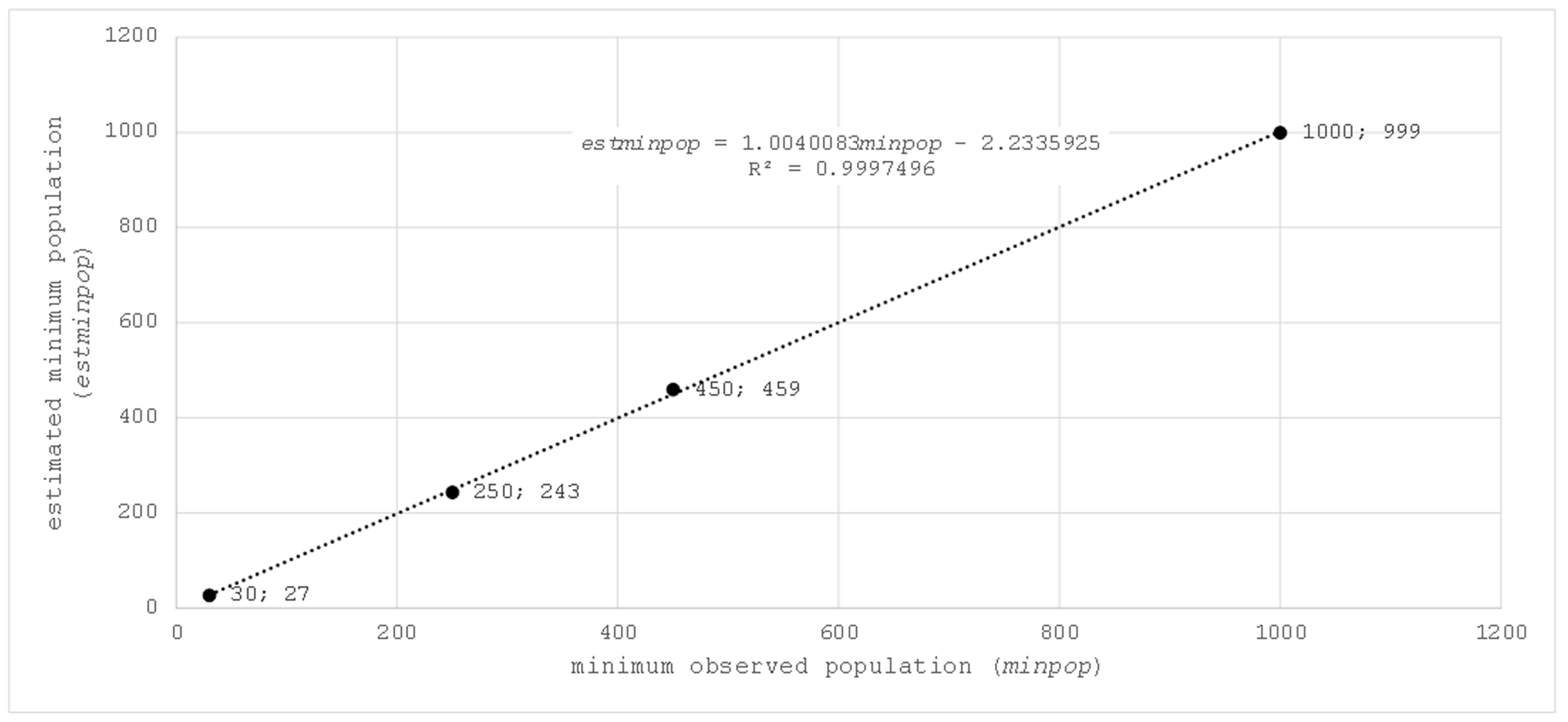
Disclaimer/Publisher’s Note: The statements, opinions and data contained in all publications are solely those of the individual author(s) and contributor(s) and not of MDPI and/or the editor(s). MDPI and/or the editor(s) disclaim responsibility for any injury to people or property resulting from any ideas, methods, instructions or products referred to in the content. |
© 2023 by the authors. Licensee MDPI, Basel, Switzerland. This article is an open access article distributed under the terms and conditions of the Creative Commons Attribution (CC BY) license (https://creativecommons.org/licenses/by/4.0/).