Article

A Novel Interpretable Deep Learning Model for Ozone Prediction

1
Jiangsu Key Laboratory of Big Data Security & Intelligent Processing, Nanjing University of Posts and Telecommunications, Nanjing 210023, China
2
School of the Environment, Nanjing University, Nanjing 210046, China
3
School of Environment, Nanjing Normal University, Nanjing 210023, China
*
Author to whom correspondence should be addressed.
These authors contributed equally to this work.
Appl. Sci. 2023, 13(21), 11799; https://doi.org/10.3390/app132111799
Submission received: 17 September 2023 / Revised: 23 October 2023 / Accepted: 26 October 2023 / Published: 28 October 2023

Abstract

:
Due to the limited understanding of the physical and chemical processes involved in ozone formation, as well as the large uncertainties surrounding its precursors, commonly used methods often result in biased predictions. Deep learning, as a powerful tool for fitting data, offers an alternative approach. However, most deep learning-based ozone-prediction models only take into account temporality and have limited capacity. Existing spatiotemporal deep learning models generally suffer from model complexity and inadequate spatiality learning. Thus, we propose a novel spatiotemporal model, namely the Spatiotemporal Attentive Gated Recurrent Unit (STAGRU). STAGRU uses a double attention mechanism, which includes temporal and spatial attention layers. It takes historical sequences from a target monitoring station and its neighboring stations as input to capture temporal and spatial information, respectively. This approach enables the achievement of more accurate results. The novel model was evaluated by comparing it to ozone observations in five major cities, Nanjing, Chengdu, Beijing, Guangzhou and Wuhan. All of these cities experience severe ozone pollution. The comparison involved Seq2Seq models, Seq2Seq+Attention models and our models. The experimental results show that our algorithm performs 14% better than Seq2Seq models and 4% better than Seq2Seq+Attention models. We also discuss the interpretability of our method, which reveals that temporality involves short-term dependency and long-term periodicity, while spatiality is mainly reflected in the transportation of ozone with the wind. This study emphasizes the significant impact of transportation on the implementation of ozone-pollution-control measures by the Chinese government.

1. Introduction

Ozone ( O 3 ) is formed through photochemical reactions of compounds (VOCs) and NO x [1]. This disparity in spatiotemporal distribution is primarily caused by variations in emission characteristics, synoptic conditions, topographic distribution and land-use types [2,3,4,5,6]. Generally, the emission source and meteorological characteristics are the fundamental and essential factors for the formation, transport and dispersion of O 3 [7]. The source of O 3 precursor emissions can be categorized as anthropogenic sources and natural sources [8]. Additionally, meteorological variables such as solar radiation, wind direction, wind speed, atmospheric pressure, temperature and relative humidity have a complex relationship with O 3 [9,10,11,12,13]. Recently, ozone pollution has gradually increased and become a primary pollutant of great concern in air pollution control [14,15,16] due to its detrimental impacts on both human health and agriculture [17,18,19,20]. Considering the complexity of the O 3 formation mechanism, the exacerbated combined atmospheric pollution increases the difficulty in ozone control [21]. One of the most important tasks for assessing efficient prevention and control strategies for O 3 pollution is predicting O 3 . Building precise O 3 -prediction models can strongly support decision-makers in efficiently reducing heavy ozone pollution peaks, which is an urgent and necessary task.
Generally, ozone-prediction approaches can be classified into two types: numerical and statistical approaches. Numerical approaches simulate the real atmospheric environment by utilizing accurate estimations of anthropogenic emissions and incorporating specific atmospheric physics and chemistry reactions. Some numerical approaches [22,23,24] have been widely used in ozone prediction. Unfortunately, numerical models suffer from an imperfect understanding of complex ozone formation and thus sacrifice spatiotemporal resolution. Therefore, the spatiotemporal representativeness, emission and modeling mechanisms still need to be perfected [25]. In contrast, statistical models do not take into account the complicated reaction mechanisms. However, they offer greater flexibility and more computing advantages [26]. Classical statistical ozone-prediction models mainly consist of basic regression models [27,28,29,30,31], which can limit the model’s capacity to describe non-linear and complex internal physicochemical processes. Therefore, they often fail to meet practical requirements [32,33]. Machine learning (ML) methods, as a promising approach, have inspired advancements in the field of ozone forecasting. Basic ML algorithms [34,35], advanced ensemble algorithms [36,37,38,39] and artificial neural network (ANN) [40,41,42] have been intensively studied in ozone forecasting. Nevertheless, these models fail to capture spatial and temporal information simultaneously and normally ignore the interaction between elements in the sequence due to their independent and identically distributed (i.i.d.) premise. Therefore, more powerful methods are needed.
To capture spatiotemporal information, emerging deep learning (DL) models are a good choice because of their powerful representative capabilities. Theoretically, a deep learning neural network (DNN) is capable of fitting any form of function. However, training such a deep neural network can be extremely challenging. Considering the No Free Lunch theorem [43,44], the majority of sequence-oriented neural networks have been implemented using the recurrent neural network (RNN) [45]. RNNs are specifically designed for sequence forecasting by learning temporal patterns. Nonetheless, RNNs have issues with gradient explosion and gradient vanishing and they also lack long-term memory. Accordingly, the Long Short-Term Memory (LSTM) [46] and Gated Recurrent Unit (GRU) [47] were proposed to address these issues by incorporating memory units and a gating mechanism [48]. The LSTM and GRU are commonly used in ozone prediction in conjunction with the Encoder–Decoder framework [49]. However, the performance of the Encoder–Decoder is limited by the fixed length of the hidden state. The presence of an attention mechanism [50] breaks the bottleneck of the Encoder–Decoder. With the attention mechanism, certain methods [51,52] can achieve more accurate results. Besides temporal features, spatial factors are also crucial. Ozone pollution is typically a regional air quality concern. Therefore, it is influenced not only by local emissions and meteorological conditions but also by the long-range transportation of ozone and its precursors [53,54]. Several deep learning-based networks are widely used to capture spatial information. The CNN can learn shift-invariant features of data because the kernel remains constant during convolution operations. Some researchers have utilized CNN models to analyze images and forecast air pollutant concentrations [55,56]. However, it is the shared parameters that make the CNN take all monitoring stations as identical within a single convolution. The attention mechanism serves the purpose of learning spatial relationships more directly by assigning different weights to each site. Some methods have been investigated, such as [57], that learn spatiotemporal information from a pre-organized feature matrix. It then applies LSTM and Multilayer Perceptron (MLP) to assign weights in the temporal and spatial dimensions to forecast PM 2.5 . Spatiality is an inherent characteristic of graph neural networks, which treats each monitoring station as a node in an undirected graph, with edges representing connections between the nodes The value of an edge indicates the strength of the connection. Using GCNs to forecast air pollutants requires performing convolution in the spectral space, which demands substantial computational power. Furthermore, the initial issue when predicting ozone with GCNs is defining the relationship between two randomly selected monitoring stations.
In this paper, we propose a novel method called the Spatiotemporal Attentive Gated Recurrent Unit (STAGRU) based on the Seq2Seq model and the attention mechanism. Our method aims to predict local ozone concentration in five mega cities across China suffering severe ozone pollution. We utilize spatiotemporal information obtained from in situ observations to improve the precision of our predictions. STAGRU applies two types of attention mechanisms. One captures temporal knowledge from historical data using an RNN-based network, while the other selects a significant moment from the historical data in the surrounding sites for the current prediction. Due to its ability to learn directly from historical data, the proposed model has a lower computational burden and higher interpretability. Details regarding model construction and the data used for training and experimental comparisons are presented in Section 2. Subsequently, we conducted experiments to compare STAGRU with Seq2Seq and Seq2Seq+Attention-based models. Finally, we will discuss the interpretability of STAGRU, which offers us insights into temporality and spatiality. Furthermore, a derivative model called STAGRU-Decoder is proposed, which predicts ozone concentration for multiple stations simultaneously.

2. Materials and Methods
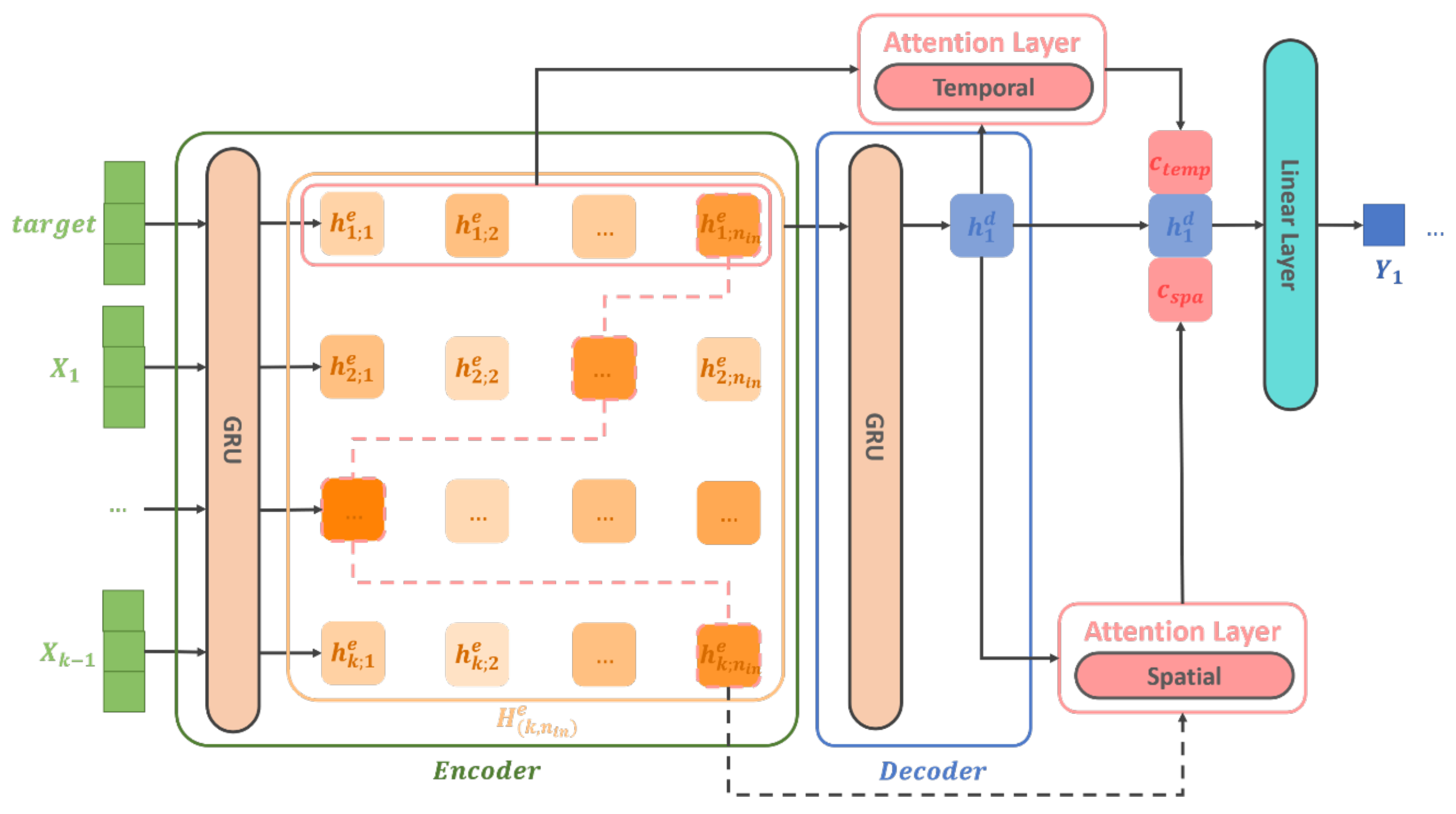
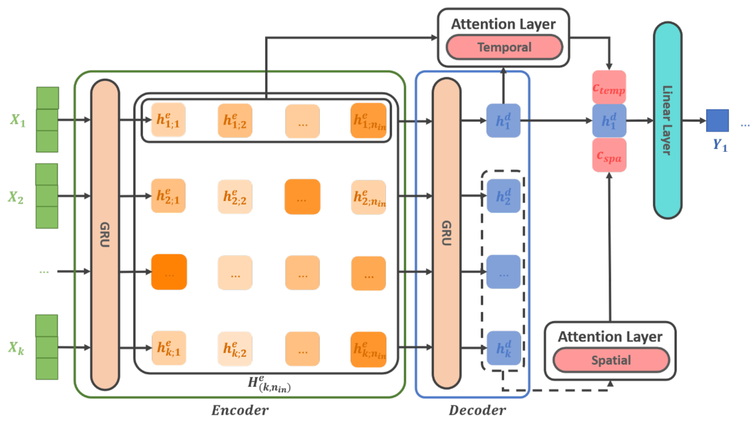
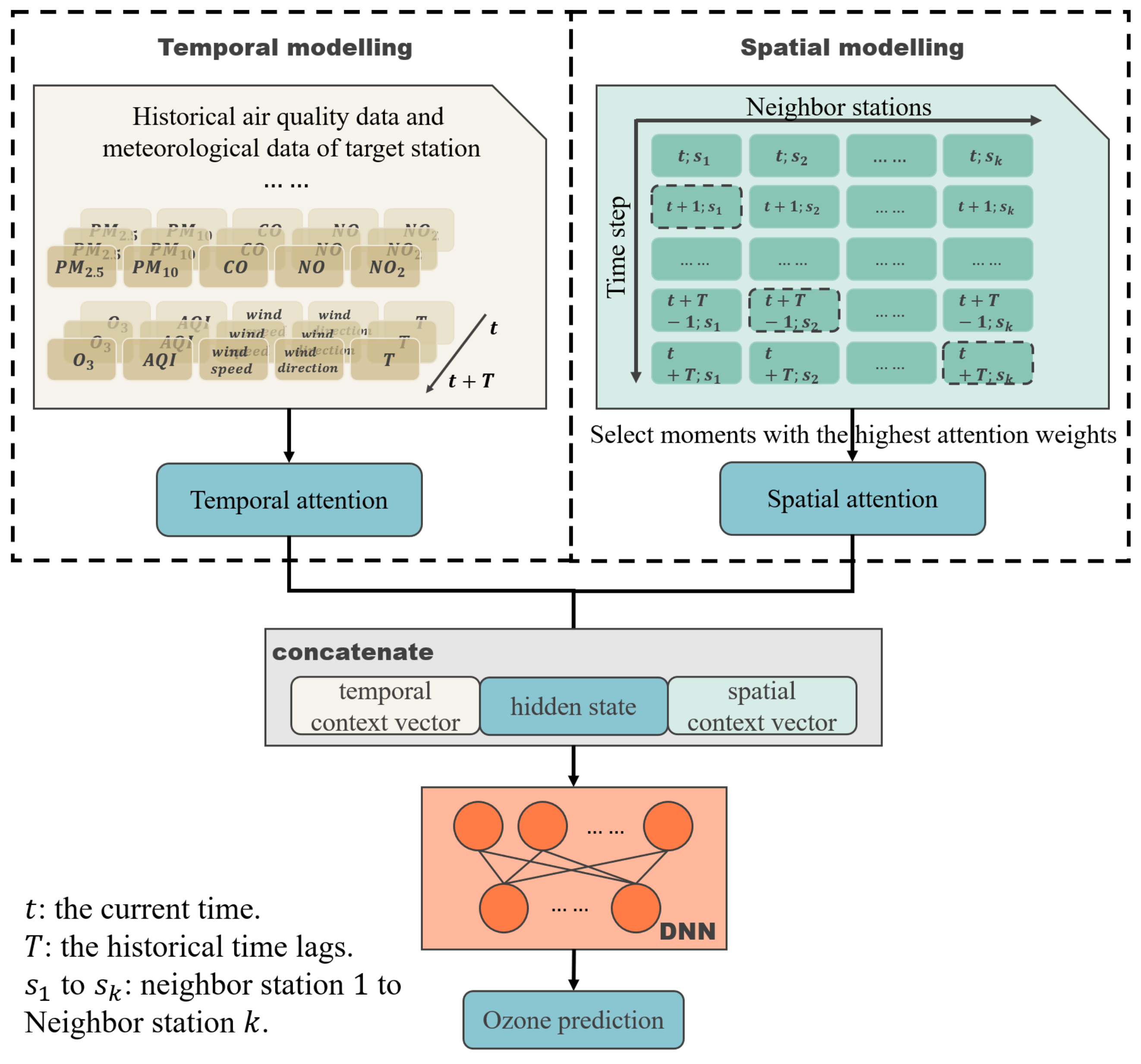
2.1. Methods

The attention mechanism is commonly used in various domains and is effective in solving sequence-prediction problems. To learn temporality, we incorporated the attention mechanism to capture the temporal information from the previous sequence of the target monitoring station. Specifically, the past sequence is sent to the temporal attention layer and the corresponding attention weight vector quantifying the relation between each past moment and current prediction is obtained. After computing the dot product of the past sequence and the attention weight vector, temporal information, namely the temporal context vector, is derived. Intrinsically, by using temporal attention, we established a link between the present prediction and every previous moment. With this connection, the knowledge from previous sequences can assist in forecasting. This inspired us to employ the idea of using the attention mechanism to construct bridges that facilitate the flow of information between multiple stations in spatial learning.
When predicting ozone for a certain station, we believe that its surrounding stations can provide assistance to improve prediction accuracy, because ozone pollution is usually a regional air quality issue. Thus, we learned spatial information from some specific moments in the past sequence of each surrounding station. Here, we propose to employ particular moments, not the whole sequence as it can reduce computation and alleviate disturbances from unimportant moments. We utilized the temporal attention layer to select the past moment with the highest attention weight for each station and introduced another attention layer, the spatial attention layer, to calculate the spatial context vector. The reason we used the temporal attention layer to make selections is that this layer contains knowledge about how to evaluate the importance of a past moment compared to the current prediction concerning the target station. Thus, the attention layer with learnable parameters is recommended. After determining these specific moments, the spatial attention layer calculates the attention score using decoding hidden states and the geographical location of that neighboring monitoring station for each selected moment to obtain the spatial context vector. In this manner, the spatial attention layer builds a connection between the target station and its neighbors and the knowledge of the past sequences of each station eventually affects the prediction.
Along with learning the temporal and spatial information, the spatiotemporal attention-based STAGRU (Spatiotemporal Attentive Gated Recurrent Unit) model was proposed. Details of the STAGRU are shown in Figure 1. As shown in Figure 1, there are two modeling parts in the STAGRU. Historical air quality data and meteorological data of the target station are fed into the Encoder and encoded into the hidden states. A temporal context vector is derived from those hidden states by the temporal attention layer when decoding. For spatial modeling, the decoding hidden states with the highest attention weight are selected to learn the spatial knowledge and obtain the spatial context vector. After this, the temporal and spatial context vectors are concatenated with the current decoding hidden state and sent to the DNN to make a prediction.

2.2. Data

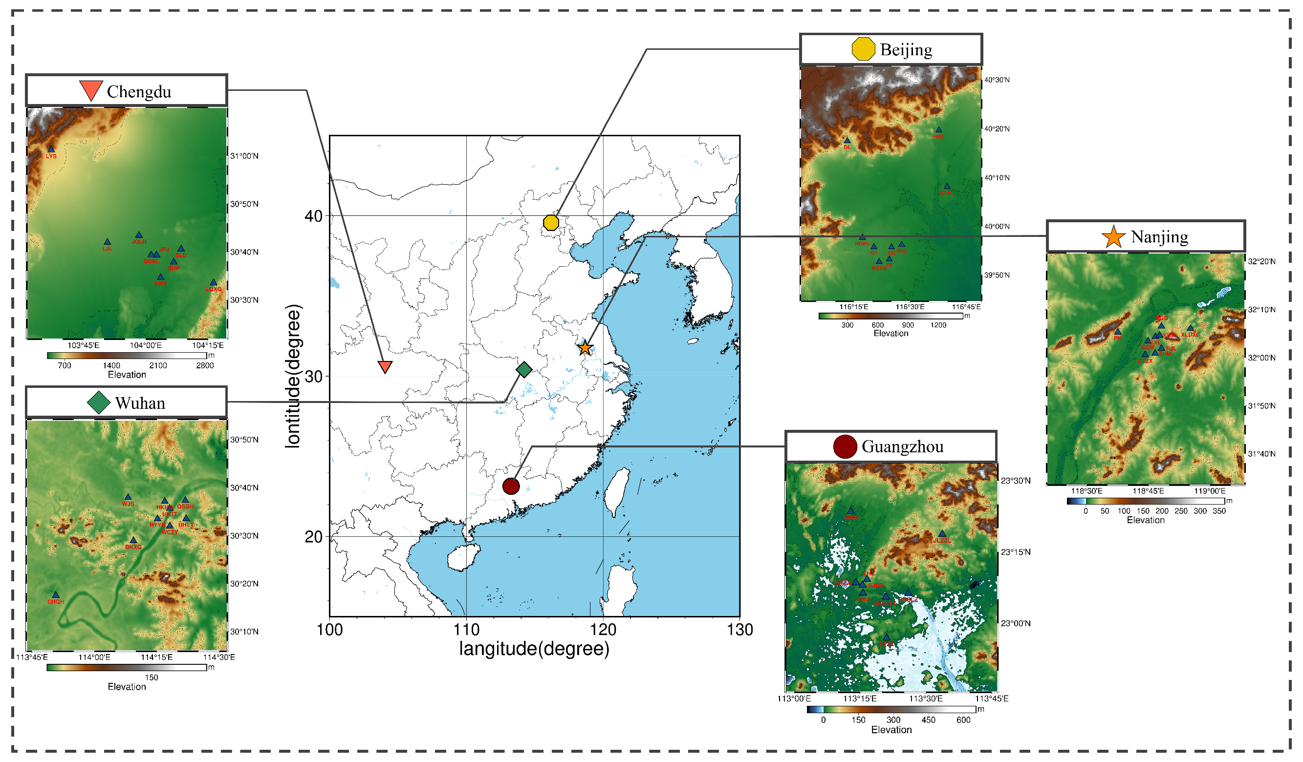
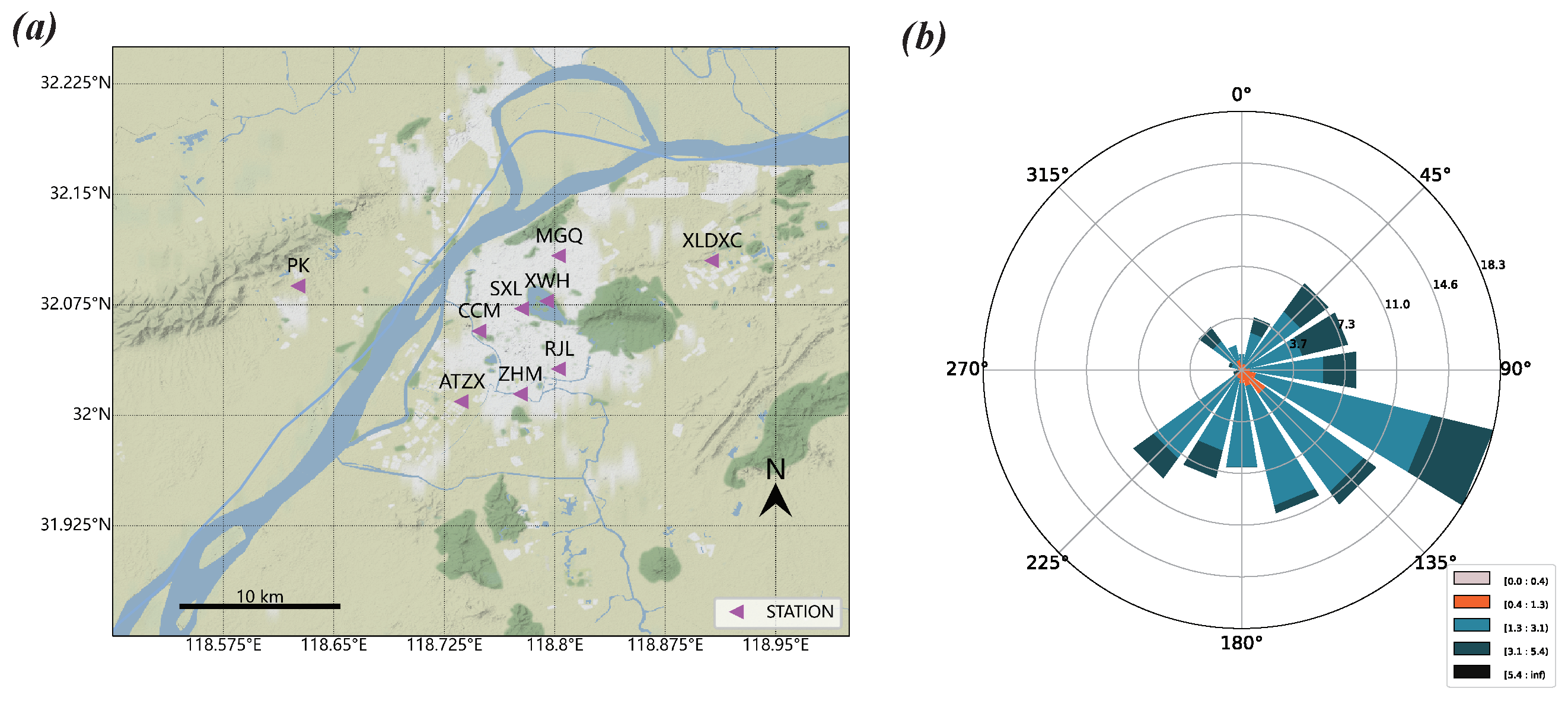
2.2.1. Study Regions and Datasets

Ozone pollution is generally a regional issue, so we selected nine monitoring stations in several cities (Nanjing, Beijing, Chengdu, Guangzhou and Wuhan) that suffer from severe ozone pollution to represent the corresponding regions. The data used in our experiments comprised the air quality (including AQI, PM 2.5 , PM 10 , SO 2 , NO 2 , O 3 and CO) and meteorological (including radial wind, temperature, relative humidity and Residual Boundary Layer Height) data of those monitoring stations from January 2015 to December 2021. The longitude and latitude of each monitoring station in each city are shown in Table A1 and the geographical distribution of these monitoring stations is shown in Figure 2. These stations were distributed in different regions of their city, like the teaching area, downtown area, industrial area, etc.
The air quality data included the hourly PM 2.5 , PM 10 , NO 2 , CO and SO 2 concentrations and the air quality index (AQI). The meteorological information included ERA5 near-surface wind speed, wind direction, temperature, relative humidity and planetary boundary layer height. In each monitoring station, we took the data from January 2015 to December 2020 as the training data and January 2021 to December 2021 as the testing data, which was used to evaluate the performance of the final trained model. Linear interpolation [58] was used to fill in the missing data, because linear interpolation is simple and able to mostly reserve statistical features of original data [59]. Normalization was applied to the air quality, wind speed and temperature data to achieve a faster convergence. We transformed the raw dataset into a supervised dataset, consisting of input–output pairs based on a sliding window. For details of the data flow, we took the past 24 h air quality and meteorological data from all stations in a city as the input. Subsequently, 24 h O 3 forecasts of the target station were obtained via the STAGRU.

2.2.2. Evaluation Metrics

In this study, the Root Mean Squared Error (RMSE), R 2 and the Symmetric Mean Absolute Percentage Error (SMAPE) were used as the performance metrics. The formula of the RMSE is shown below
RMSE = i = 1 n ( y i y ^ i ) 2 n
where y i represents the observation of item i; y ^ i represents the prediction of item i; and n represents the number of items. R 2 measures the fitting degree between the model and the true state. The formula is defined as follows:
R 2 = 1 i = 1 n ( y i y ^ i ) 2 i = 1 n ( y i y ¯ ) 2
where y ¯ = i = 1 n y i .
The SMAPE measures the accuracy of the predictions based on percentage error, which is defined as follows:
SMAPE = 100 % n i = 0 n | y ^ i y i | ( | y ^ i | + | y i | ) / 2
Note that each evaluation metric above has its advantages and disadvantages; thus, we integrated different approaches to measure the effectiveness of the model.

2.2.3. Experimental Design
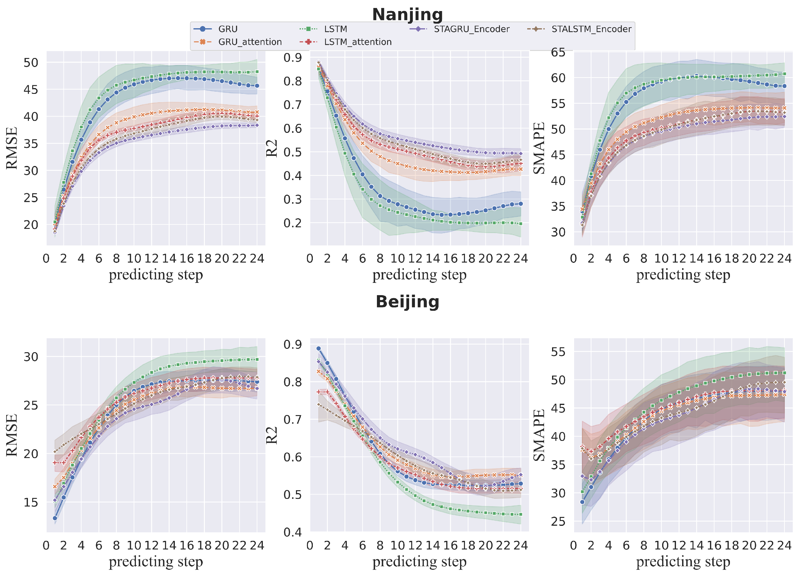
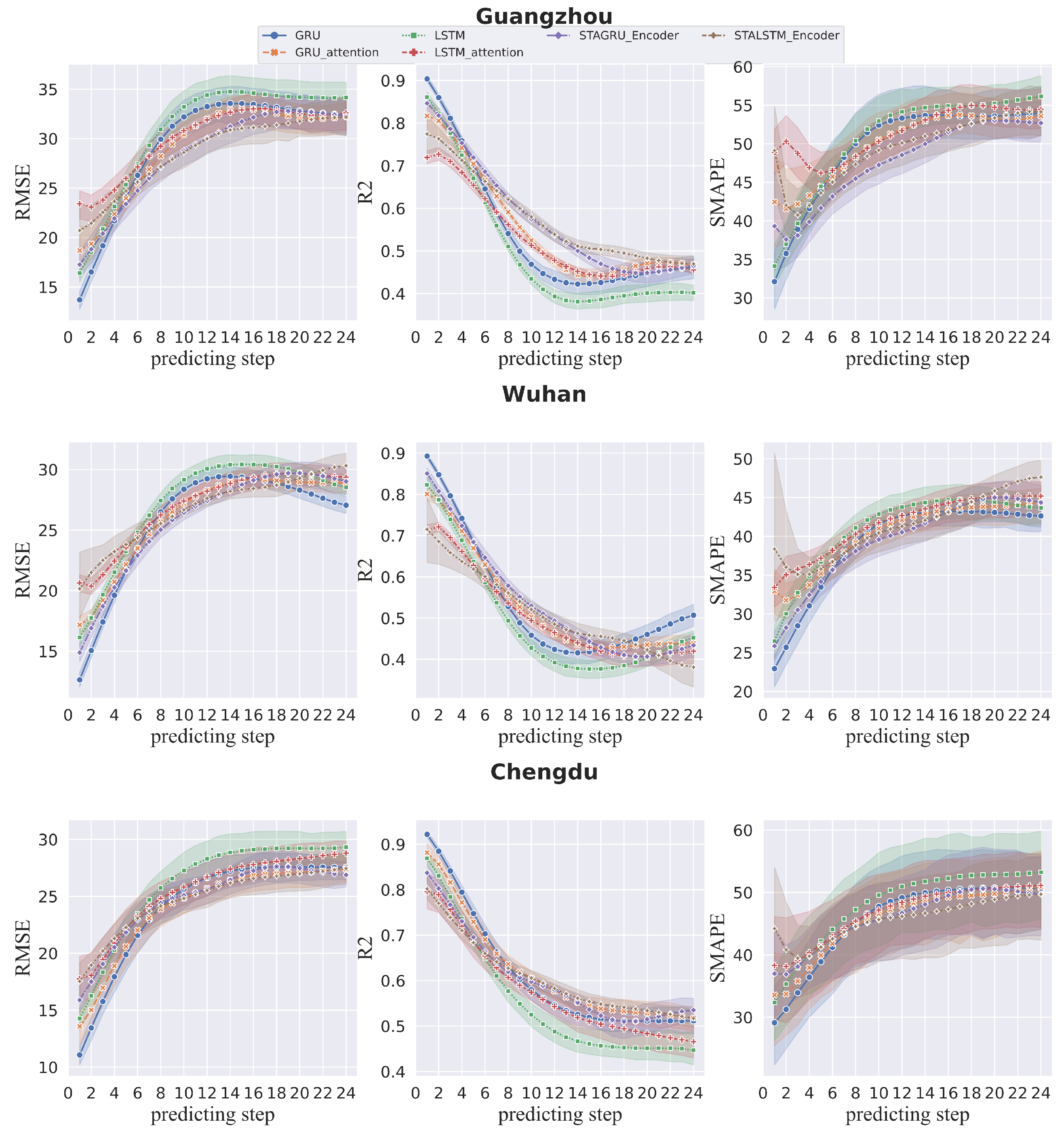
In order to evaluate the capability of the STAGRU, we compared it with the Seq2Seq- and Seq2Seq+Attention-based models. Further, we also considered adopting LSTM to replace GRU in the STAGRU, producing an STALSTM, because these two RNN methods are frequently used in many time series prediction tasks [60,61]. The details of the experimental design are shown in Table 1. The number of hidden units was 256, the hidden layer was 1, the batch size was 48 and the optimizer was Adam [62] and the learning rate was 0.0001. Early stopping was applied to obtain an acceptable model, and schedule sampling was also used. Further, all experiments were conducted on an NVIDIA GeForce GTX 1050Ti 4G GPU.

3. Results

We executed the six models mentioned above in each monitoring station in each city to predict the ozone levels in the subsequent 24 h. In each station, all models were trained and tested on the same training and testing datasets, respectively. The RMSE, R2 and SMAPE of each model from the nine stations are shown in Figure 3 and Figure 4.
Figure 3 shows the performance of each model in the Nanjing and Beijing cities, while Figure 4 shows the performance of each model in Guangzhou, Wuhan and Chengdu. The comparisons between the different types of models and between LSTM and GRU within each model were then analyzed. As shown in the two figures, the performance of all these models declines in the early stages and then gradually becomes stable after 12 h. As shown in the figures, the Seq2Seq-based model performed well in the early prediction stage, then it rapidly declined. Comparing LSTM and GRU, GRU generally performed better than LSTM. As for the Seq2Seq+Attention-based model, the performance was more stable and errors accumulated more slowly than the Seq2Seq-based models. Considering our spatiotemporal-based model, the STAGRU performed best in the Nanjing and Beijing cities. The two spatiotemporal models performed similarly and made better predictions than the other models in the Chengdu, Guangzhou and Wuhan cities.
Generally, the error of the RNN-based models, especially under the Encoder–Decoder framework, accumulates as the forecast time increases; this is because the relevance between the past observation values and prediction values becomes weaker and thus the recursivity of the Encoder–Decoder framework makes further errors. The predictions of the Seq2Seq-based methods are generally adequate during the early forecasting hour; however, they begin to deteriorate at a much faster rate than the other methods as forecast time increases. The reason for this is that the only connection between the prediction and the past sequence is the last decoding hidden state, which cannot afford enough information to support forecasting due to the fixed length of the hidden state, thus making errors accumulate rapidly. Therefore, the fitting ability of the Seq2Seq-based model is unsatisfactory. The Seq2Seq+Attention-based methods introduce the attention mechanism to link each prediction with all past moments, which complements the shortage of Seq2Seq-based methods and generates a better model with improved performance. With the support of temporal information, Seq2Seq+Attention-based methods can significantly improve forecasting skills. However, Seq2Seq+Attention-based methods fluctuate as forecasting goes on. This is because the attention mechanism in the Seq2Seq+Attention-based models tends to learn periodicity from past sequences and the periodicity can be vulnerable to error accumulation which makes the model less dynamic. Spatiotemporal attentive-based methods bring an extra attention layer, similar to Seq2Seq+Attention, to make a connection between the observations of the spatially distributed stations.
In summary, Seq2Seq-based models are only sufficient to solve short-term sequence predictions due to their limited representation capabilities and fast error accumulation. Attention mechanisms can reinforce Seq2Seq, but the information they capture is still insufficient. Spatiotemporal attentive-based methods generally perform better than other models due to the spatiotemporal information learned, which improves the fitting ability and robustness of the models. Moreover, to demonstrate the adaptability of GRU and LSTM to the spatiotemporal attention mechanism, we compared the STAGRU and the STALSTM. The results showed that the GRU is a better choice than LSTM for our proposed model.

4. Discussion

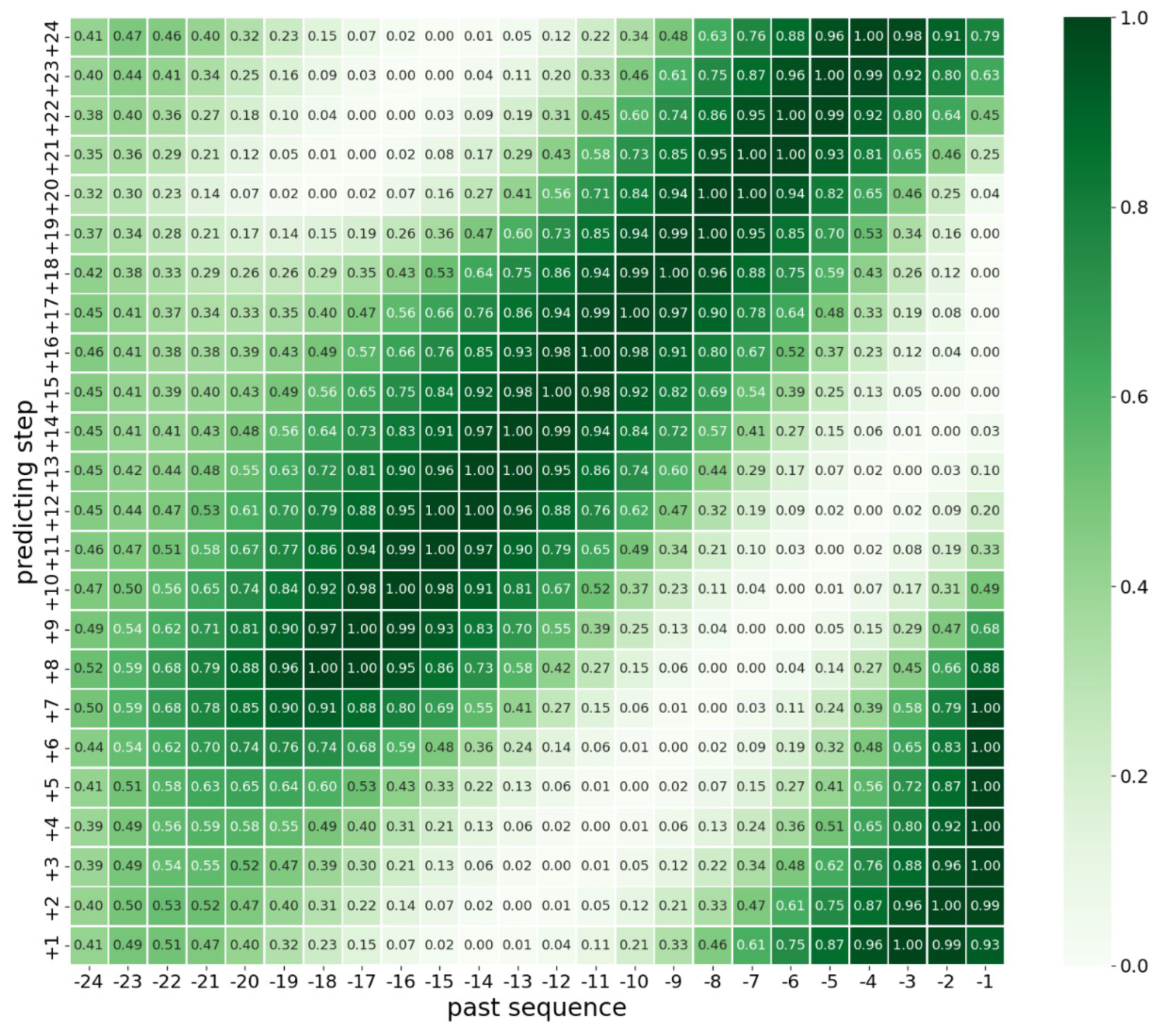
4.1. Interpretability Discussion

Another important issue in O 3 prediction is how to interpret the results. For this purpose, we took the nine monitoring stations in Nanjing city as our analysis target. July 2019 was chosen for the interpretability discussion because of the generally consistent wind direction of the selected monitoring stations during this period. We collated the hourly data into a supervised dataset and 697 samples were obtained. The geographical distribution of the nine monitoring stations is shown in Figure 5a. The wind speed (classified based on the Beaufort wind scale) and wind direction distribution of all stations during this period are shown in Figure 5b. From Figure 5b, it can be seen that the dominant wind direction in July 2019 was ESE and the wind speed was between 1.3 m s 1 and 3.1 m s 1 .
For the interpretability discussion of temporality, we reviewed how the temporal attention layer assigns weights to each past moment; some statistical procedures were then conducted. The statistical process was conducted in two steps as follows: (1) We computed the summation of the temporal attention weight using all samples in July 2019. A 24 × 24 matrix representing the sum of the attention weight for each forecast time and past moment was constructed. (2) The min-max normalization was applied to the matrix to highlight the relative importance of each past moment to the prediction of the target station at each forecast time (the closer the value is to 1, the more important the past moment is to the corresponding prediction step and vice versa).
As shown in Figure 6, the temporal attention layer tends to learn the short-term dependency in the prediction of the first several hours. Specifically, in the prediction of the 1 st to 4 th hour, the temporal attention layer assigns the largest weight to the 4 th to 1 st past moments and the Pearson correlation coefficient between the prediction steps and the most important moments was 0.94 (Figure 6). As the forecast lead time increases, the short-term dependency gradually shifts to periodical dependency. According to Figure 6, the periodical dependency dominates from the 8 th to the last prediction step and the corresponding most important past moment is from the 18 th to the 4 th . The Pearson correlation coefficient was 0.99, which means a highly positive correlation (Figure 6). In summary, the temporal information was learned in short-term and periodical dependency and the temporal attention finely captured the trade-off of these two kinds of dependency.
For the interpretability discussion of how the predictions of the target station are affected by stations nearby in the STAGRU, the same statistical procedures were conducted. We computed the summation of the attention weight for each prediction step of each surrounding monitoring station in July 2019. A 24 × 8 matrix representing the relation between each forecast lead time and surrounding stations was created. The statistical results of the station CCM (located in the middle of the study area) are depicted in Figure 7. According to the heat map, it is obvious that the RJL is the most important surrounding monitoring station to the CCM for the whole prediction, which is consistent with their relative geolocation and the dominant wind direction. XWH, SXL, ZHM and ATZX are also important; a certain number of NE, ENE, ESE and SW winds were present according to Figure 5b. According to Figure 5a, it can be seen that a mountain stands upwind of the station MGQ, which weakens the airflow and reduces the wind. Further, the relative humidity of the Xuanwu Lake is significant, which negatively influences ozone formation [10]. Meanwhile, MGQ is located downwind. Consequently, the station MGQ becomes the least important neighbor. Empirically, we remove the data of station MGQ and then evaluate the performance. Before eliminating station MGQ, the average RMSE, R 2 and SMAPE in station CCM were 34.83, 0.59 and 48.55, respectively. After removing station MGQ, the average RMSE, R 2 and SMAPE were 35.18, 0.59 and 49.09, respectively. Thus, the performance attenuation was slight.
In summary, on the one hand, the interpretable results are consistent with the actual findings, which investigated the reliability of our proposed model; on the other hand, analyzing the inner mechanism of the model continuously deepened and strengthened the presence of spatiality. Concretely, distance is not the only important factor influencing pollutant transmission; the results also show that the wind direction matters. Thus, future work concerning spatial prediction should pay more attention to utilizing additional spatial information, like wind direction, etc.

4.2. Derivative Model Discussion

In this study, we designed a model that learns spatial information from the encoding hidden states (Figure A1). However, spatial information can be also captured during decoding. Based on the STAGRU, we moved the spatial information learning process from the encoding hidden states of past sequences of each monitoring station to the decoding hidden states of each station that are in the same prediction step (namely STAGRU-Decoder). The details of this model are shown in Figure A2. Firstly, it is clear that the spatial attention layer of the STAGRU-Decoder receives the decoding hidden states of all monitoring stations in the same prediction step. Then, all stations make predictions simultaneously during decoding. In this manner, the STAGRU-Decoder can achieve synchronous prediction for multiple monitoring stations, which reduces the model training overhead.
We investigated the effectiveness of the STAGRU-Decoder by comparing it with the STAGRU in five cities. The results are shown in Figure A3. According to the results, the mean performance of the STAGRU-Decoder is better than the STAGRU in Beijing and Guangzhou and it performed similarly in other cities. However, the STAGRU-Decoder becomes unstable as the forecast lead time increases, after the 8th hour specifically, according to the undertint area. We considered that the predictions made by the STAGRU-Decoder for the monitoring stations are built on the predictions of others, which causes error superposition. Thus, the stability of the STAGRU-Decoder deteriorates as forecasting continues. Furthermore, we note that the applicable scope of the spatial information learning in the STAGRU and STAGRU-Decoder is limited by the wind force, where the air pollutant is transported more widely when the wind becomes stronger.

5. Conclusions

In this paper, we propose a novel model called the Spatiotemporal Gate Recurrent Unit (STAGRU), which captures spatiotemporal information using two types of attention mechanisms: temporal attention and spatial attention. Temporal attention captures information from the past sequence, while spatial attention captures information from the surrounding monitoring stations. We demonstrated the effectiveness of the STAGRU model compared to Seq2Seq and Seq2Seq+Attention models in five major cities: Nanjing, Beijing, Wuhan, Guangzhou and Chengdu. Statistically, our proposed method is 14% better than Seq2Seq-based methods and 4% better than Seq2Seq+Attention-based methods. Furthermore, we proposed another model that captures spatial information during decoding. This model was able to apply forecasting to multiple stations simultaneously, but it came at the cost of stability. In addition, it provided insight into our proposed model, enabling a discussion on interpretability from the perspective of statistical temporality and spatiality. The analysis shows that the temporality of ozone variation involves short-term dependency and long-term periodicity and that the spatiality of ozone transportation is mainly affected by wind, including speed and direction. By utilizing our model, policy decision-makers can make accurate ozone predictions in advance for specific regions of interest. If it is predicted that there will be ozone pollution in this area, decision-makers can provide early warnings and take appropriate measures to control the area. Current results presented in this manuscript are considered preliminary. For future work, the two major objectives are to extend the domain by including more observational stations (e.g., mainland China) and to further improve accuracy. It is worth noting that the amount of CPU time required for the calculation is directly proportional to the number of monitoring stations being considered. This implies that larger domain tests necessitate significant computational resources.

Author Contributions

X.C.: Conceptualization, Writing—review and editing and supervision. Y.L.: conceptualization, methodology, validation, investigation, data curation, writing—original draft and visualization. X.X.: methodology, investigation, writing—original draft, visualization and data curation. M.S.: writing—review and editing, resources and supervision. All authors have read and agreed to the published version of the manuscript.

Funding

This paper was partially supported by the National Natural Science Foundation of China (No.62276142, 62206133, 62202240, 62192783), the Special Science and Technology Innovation Program for Carbon Peak and Carbon Neutralization of Jiangsu Province (No. BE2022612), and the Natural Science Foundation of Jiangsu Province (No. BK20210574).

Institutional Review Board Statement

Not applicable.

Informed Consent Statement

Not applicable.

Data Availability Statement

The data presented in this study are openly available in FigShare accessed on 18 September 2023. Li, Yang (2023). Air pollutant and meteorological data of five major cities in China. figshare. Dataset. https://doi.org/10.6084/m9.figshare.24152163.v2.

Conflicts of Interest

The authors declare no conflict of interest.

Appendix A

This appendix contains three parts as follows: a detailed neural network structure of the proposed model in two versions; the performance comparison between the two version of the model; the geolocation of all the monitoring stations in each city.
Figure A1. The structure of the STAGRU. The target represents the past sequence of the target station, while X i represents the past sequence of the surrounding station i. Sending data to the Encoder, the GRU component encodes each moment into a hidden state and a hidden state matrix is produced, named H ( k , n i n ) e . Note, the row and column of H ( k , n i n ) e depends on the number of stations and the length of each past sequence. The last encoding hidden state of the target sequence is fed into the Decoder. With this hidden state, the Decoder produces the decoding hidden state for each prediction step. In each prediction step, the temporal context vector, derived from the encoding hidden states of the target station and the spatial context vector, derived from the encoding hidden states with the highest attention weight in each monitor station, are applied to make a prediction. Specifically, the temporal context vector, c t e m p , and the spatial context vector, c s p a , are concatenated with the current decoding hidden state, h d ; then the concatenation is sent to a linear layer to forecast Y.
Applsci 13 11799 g0a1
Figure A2. The structure of the STAGRU-Decoder. The main difference is in the spatial information learning. The STAGRU-Decoder learns the spatiality from the decoding hidden states of the other surrounding stations. This operation is applied for the prediction step of each station. In this manner, there is no target station; all stations are forecasted synchronously.
Applsci 13 11799 g0a2
Figure A3. Performance comparison between the Seq2Seq (GRU and LSTM), Seq2Seq+Attention (GRU_attention and LSTM_attention) and spatiotemporal attentive models (STAGRU_Encoder, STALSTM_Encoder, STAGRU_Decoder and STALSTM_Decoder) in Beijing, Chengdu, Guangzhou and Wuhan. The x axis represents the prediction step and the y axis represents the three criteria (RMSE, R2 and SMAPE). Solid line denotes the mean value over the nine monitoring stations in the prediction step and the shaded area is the performance variation region of a certain model.
Applsci 13 11799 g0a3
Table A1. Longitude and latitude of each selected monitoring station in Nanjing, Beijing, Chengdu, Guangzhou and Wuhan.
CityStationLongitudeLatitudeStationLongitudeLatitude
NanjingATZX118.73732.009RJL118.80332.031
CCM118.74932.057SXL118.77832.072
MGQ118.80332.108XLDXC118.90732.105
PK118.62632.088XWH118.79532.078
ZHM118.77732.014
BeijingWSXG116.362139.8784DL116.220240.2915
DS116.417439.9289TT116.407239.8863
NZG116.46239.9365GY116.339239.9295
HDWL116.287839.9611SYXC116.663640.135
HRZ116.627560.3275
ChengduJQLH103.972830.7236SLD104.141930.6764
SWY104.059430.5767SHP104.112230.6306
JPJ104.043130.6556LYS103.620231.0201
DSXL104.021930.6558LQXQ104.272530.5589
LJL103.845830.6994
GuangzhouGYZX113.234723.1423SWZ113.261223.105
GDSXY113.347823.0916SBSLZ113.433223.1047
FYZX113.350522.9483HDSF113.214623.3916
SJCZ113.259723.1331JLZZL113.561823.312
LH113.276523.1544
WuhanDHLY114.367730.5584HYYH114.252930.558
HKHQ114.28230.6189WCZY114.302530.5332
QSGH114.364630.6217DKXQ114.156630.4825
HKJT114.301430.5944WJS114.13530.6319
CHQH113.845430.2917

References

  1. Atkinson, R. Atmospheric chemistry of VOCs and NOx. Atmos. Environ. 2000, 34, 2063–2101. [Google Scholar]
  2. Carvalho, A.; Carvalho, A.; Gelpi, I.; Barreiro, M.; Borrego, C.; Miranda, A.; Pérez-Muñuzuri, V. Influence of topography and land use on pollutants dispersion in the Atlantic coast of Iberian Peninsula. Atmos. Environ. 2006, 40, 3969–3982. [Google Scholar]
  3. Meng, X.; Wang, W.; Shi, S.; Zhu, S.; Wang, P.; Chen, R.; Xiao, Q.; Xue, T.; Geng, G.; Zhang, Q.; et al. Evaluating the spatiotemporal ozone characteristics with high-resolution predictions in mainland China, 2013–2019. Environ. Pollut. 2022, 299, 118865. [Google Scholar]
  4. Tu, J.; Xia, Z.G.; Wang, H.; Li, W. Temporal variations in surface ozone and its precursors and meteorological effects at an urban site in China. Atmos. Res. 2007, 85, 310–337. [Google Scholar]
  5. Wang, W.N.; Cheng, T.H.; Gu, X.F.; Chen, H.; Guo, H.; Wang, Y.; Bao, F.W.; Shi, S.Y.; Xu, B.R.; Zuo, X.; et al. Assessing spatial and temporal patterns of observed ground-level ozone in China. Sci. Rep. 2017, 7, 3651. [Google Scholar]
  6. Yu, R.; Lin, Y.; Zou, J.; Dan, Y.; Cheng, C. Review on atmospheric ozone pollution in China: Formation, spatiotemporal distribution, precursors and affecting factors. Atmosphere 2021, 12, 1675. [Google Scholar]
  7. Mousavinezhad, S.; Choi, Y.; Pouyaei, A.; Ghahremanloo, M.; Nelson, D.L. A comprehensive investigation of surface ozone pollution in China, 2015–2019: Separating the contributions from meteorology and precursor emissions. Atmos. Res. 2021, 257, 105599. [Google Scholar]
  8. Lelieveld, J.; Dentener, F.J. What controls tropospheric ozone? J. Geophys. Res. Atmos. 2000, 105, 3531–3551. [Google Scholar]
  9. Camalier, L.; Cox, W.; Dolwick, P. The effects of meteorology on ozone in urban areas and their use in assessing ozone trends. Atmos. Environ. 2007, 41, 7127–7137. [Google Scholar]
  10. Dueñas, C.; Fernández, M.; Cañete, S.; Carretero, J.; Liger, E. Assessment of ozone variations and meteorological effects in an urban area in the Mediterranean Coast. Sci. Total Environ. 2002, 299, 97–113. [Google Scholar]
  11. Hu, C.; Kang, P.; Jaffe, D.A.; Li, C.; Zhang, X.; Wu, K.; Zhou, M. Understanding the impact of meteorology on ozone in 334 cities of China. Atmos. Environ. 2021, 248, 118221. [Google Scholar]
  12. Li, K.; Chen, L.; Ying, F.; White, S.J.; Jang, C.; Wu, X.; Gao, X.; Hong, S.; Shen, J.; Azzi, M.; et al. Meteorological and chemical impacts on ozone formation: A case study in Hangzhou, China. Atmos. Res. 2017, 196, 40–52. [Google Scholar]
  13. Pu, X.; Wang, T.; Huang, X.; Melas, D.; Zanis, P.; Papanastasiou, D.; Poupkou, A. Enhanced surface ozone during the heat wave of 2013 in Yangtze River Delta region, China. Sci. Total Environ. 2017, 603, 807–816. [Google Scholar] [CrossRef]
  14. Lu, X.; Hong, J.; Zhang, L.; Cooper, O.R.; Schultz, M.G.; Xu, X.; Wang, T.; Gao, M.; Zhao, Y.; Zhang, Y. Severe surface ozone pollution in China: A global perspective. Environ. Sci. Technol. Lett. 2018, 5, 487–494. [Google Scholar] [CrossRef]
  15. Sun, L.; Xue, L.; Wang, T.; Gao, J.; Ding, A.; Cooper, O.R.; Lin, M.; Xu, P.; Wang, Z.; Wang, X.; et al. Significant increase of summertime ozone at Mount Tai in Central Eastern China. Atmos. Chem. Phys. 2016, 16, 10637–10650. [Google Scholar]
  16. Wang, T.; Wei, X.; Ding, A.; Poon, C.N.; Lam, K.S.; Li, Y.S.; Chan, L.; Anson, M. Increasing surface ozone concentrations in the background atmosphere of Southern China, 1994–2007. Atmos. Chem. Phys. 2009, 9, 6217–6227. [Google Scholar] [CrossRef]
  17. Dimakopoulou, K.; Douros, J.; Samoli, E.; Karakatsani, A.; Rodopoulou, S.; Papakosta, D.; Grivas, G.; Tsilingiridis, G.; Mudway, I.; Moussiopoulos, N.; et al. Long-term exposure to ozone and children’s respiratory health: Results from the RESPOZE study. Environ. Res. 2020, 182, 109002. [Google Scholar]
  18. Keiser, D.; Lade, G.; Rudik, I. Air pollution and visitation at US national parks. Sci. Adv. 2018, 4, eaat1613. [Google Scholar] [CrossRef]
  19. Michaudel, C.; Mackowiak, C.; Maillet, I.; Fauconnier, L.; Akdis, C.A.; Sokolowska, M.; Dreher, A.; Tan, H.T.T.; Quesniaux, V.F.; Ryffel, B.; et al. Ozone exposure induces respiratory barrier biphasic injury and inflammation controlled by IL-33. J. Allergy Clin. Immunol. 2018, 142, 942–958. [Google Scholar]
  20. Zhang, Y.; Ma, Y.; Feng, F.; Cheng, B.; Shen, J.; Wang, H.; Jiao, H.; Li, M. Respiratory mortality associated with ozone in China: A systematic review and meta-analysis. Environ. Pollut. 2021, 280, 116957. [Google Scholar]
  21. Wennberg, P.O.; Dabdub, D. Rethinking ozone production. Science 2008, 319, 1624–1625. [Google Scholar] [CrossRef] [PubMed]
  22. Bey, I.; Jacob, D.J.; Yantosca, R.M.; Logan, J.A.; Field, B.D.; Fiore, A.M.; Li, Q.; Liu, H.Y.; Mickley, L.J.; Schultz, M.G. Global modeling of tropospheric chemistry with assimilated meteorology: Model description and evaluation. J. Geophys. Res. Atmos. 2001, 106, 23073–23095. [Google Scholar] [CrossRef]
  23. Dennis, R.L.; Byun, D.W.; Novak, J.H.; Galluppi, K.J.; Coats, C.J.; Vouk, M.A. The next generation of integrated air quality modeling: EPA’s Models-3. Atmos. Environ. 1996, 30, 1925–1938. [Google Scholar] [CrossRef]
  24. Grell, G.A.; Peckham, S.E.; Schmitz, R.; McKeen, S.A.; Frost, G.; Skamarock, W.C.; Eder, B. Fully coupled “online” chemistry within the WRF model. Atmos. Environ. 2005, 39, 6957–6975. [Google Scholar] [CrossRef]
  25. Zhou, G.; Xu, J.; Xie, Y.; Chang, L.; Gao, W.; Gu, Y.; Zhou, J. Numerical air quality forecasting over eastern China: An operational application of WRF-Chem. Atmos. Environ. 2017, 153, 94–108. [Google Scholar] [CrossRef]
  26. Schlink, U.; Herbarth, O.; Richter, M.; Dorling, S.; Nunnari, G.; Cawley, G.; Pelikan, E. Statistical models to assess the health effects and to forecast ground-level ozone. Environ. Model. Softw. 2006, 21, 547–558. [Google Scholar] [CrossRef]
  27. Huang, L.; Zhang, C.; Bi, J. Development of land use regression models for PM2.5, SO2, NO2 and O3 in Nanjing, China. Environ. Res. 2017, 158, 542–552. [Google Scholar] [CrossRef]
  28. Hubbard, M.C.; Cobourn, W.G. Development of a regression model to forecast ground-level ozone concentration in Louisville, KY. Atmos. Environ. 1998, 32, 2637–2647. [Google Scholar] [CrossRef]
  29. Kumar, U.; Jain, V. ARIMA forecasting of ambient air pollutants (O3, NO, NO2 and CO). Stoch. Environ. Res. Risk Assess. 2010, 24, 751–760. [Google Scholar] [CrossRef]
  30. Pagowski, M.; Grell, G.; Devenyi, D.; Peckham, S.; McKeen, S.; Gong, W.; Delle Monache, L.; McHenry, J.; McQueen, J.; Lee, P. Application of dynamic linear regression to improve the skill of ensemble-based deterministic ozone forecasts. Atmos. Environ. 2006, 40, 3240–3250. [Google Scholar] [CrossRef]
  31. Wang, M.; Keller, J.P.; Adar, S.D.; Kim, S.Y.; Larson, T.V.; Olives, C.; Sampson, P.D.; Sheppard, L.; Szpiro, A.A.; Vedal, S.; et al. Development of long-term spatiotemporal models for ambient ozone in six metropolitan regions of the United States: The MESA Air study. Atmos. Environ. 2015, 123, 79–87. [Google Scholar] [CrossRef] [PubMed]
  32. Comrie, A.C. Comparing neural networks and regression models for ozone forecasting. J. Air Waste Manag. Assoc. 1997, 47, 653–663. [Google Scholar] [CrossRef]
  33. Robeson, S.; Steyn, D. Evaluation and comparison of statistical forecast models for daily maximum ozone concentrations. Atmos. Environ. Part B Urban Atmos. 1990, 24, 303–312. [Google Scholar] [CrossRef]
  34. Burrows, W.R.; Benjamin, M.; Beauchamp, S.; Lord, E.R.; McCollor, D.; Thomson, B. CART decision-tree statistical analysis and prediction of summer season maximum surface ozone for the Vancouver, Montreal and Atlantic regions of Canada. J. Appl. Meteorol. Climatol. 1995, 34, 1848–1862. [Google Scholar] [CrossRef]
  35. Luna, A.; Paredes, M.; De Oliveira, G.; Corrêa, S. Prediction of ozone concentration in tropospheric levels using artificial neural networks and support vector machine at Rio de Janeiro, Brazil. Atmos. Environ. 2014, 98, 98–104. [Google Scholar] [CrossRef]
  36. Cai, W. Using machine learning method for predicting the concentration of ozone in the air. Environ. Conform. Assess 2018, 10, 78–84. [Google Scholar]
  37. Ding, S.; Chen, B.; Wang, J.; Chen, L.; Zhang, C.; Sun, S.; Huang, C. An applied research of decision-tree based statistical model in forecasting the spatial-temporal distribution of O3. Acta Sci. Circumst. 2018, 38, 3229–3242. [Google Scholar]
  38. Eslami, E.; Salman, A.K.; Choi, Y.; Sayeed, A.; Lops, Y. A data ensemble approach for real-time air quality forecasting using extremely randomized trees and deep neural networks. Neural Comput. Appl. 2020, 32, 7563–7579. [Google Scholar] [CrossRef]
  39. Requia, W.J.; Di, Q.; Silvern, R.; Kelly, J.T.; Koutrakis, P.; Mickley, L.J.; Sulprizio, M.P.; Amini, H.; Shi, L.; Schwartz, J. An ensemble learning approach for estimating high spatiotemporal resolution of ground-level ozone in the contiguous United States. Environ. Sci. Technol. 2020, 54, 11037–11047. [Google Scholar] [CrossRef]
  40. Al-Alawi, S.M.; Abdul-Wahab, S.A.; Bakheit, C.S. Combining principal component regression and artificial neural networks for more accurate predictions of ground-level ozone. Environ. Model. Softw. 2008, 23, 396–403. [Google Scholar] [CrossRef]
  41. Arhami, M.; Kamali, N.; Rajabi, M.M. Predicting hourly air pollutant levels using artificial neural networks coupled with uncertainty analysis by Monte Carlo simulations. Environ. Sci. Pollut. Res. 2013, 20, 4777–4789. [Google Scholar] [CrossRef]
  42. Tsai, C.H.; Chang, L.C.; Chiang, H.C. Forecasting of ozone episode days by cost-sensitive neural network methods. Sci. Total Environ. 2009, 407, 2124–2135. [Google Scholar] [CrossRef] [PubMed]
  43. Wolpert, D.H. The lack of a priori distinctions between learning algorithms. Neural Comput. 1996, 8, 1341–1390. [Google Scholar] [CrossRef]
  44. Wolpert, D.H.; Macready, W.G. No free lunch theorems for optimization. IEEE Trans. Evol. Comput. 1997, 1, 67–82. [Google Scholar] [CrossRef]
  45. Elman, J.L. Finding structure in time. Cogn. Sci. 1990, 14, 179–211. [Google Scholar] [CrossRef]
  46. Lipton, Z.C.; Berkowitz, J.; Elkan, C. A critical review of recurrent neural networks for sequence learning. arXiv 2015, arXiv:1506.00019. [Google Scholar]
  47. Chung, J.; Gulcehre, C.; Cho, K.; Bengio, Y. Empirical evaluation of gated recurrent neural networks on sequence modeling. arXiv 2014, arXiv:1412.3555. [Google Scholar]
  48. Pascanu, R.; Mikolov, T.; Bengio, Y. On the difficulty of training recurrent neural networks. In Proceedings of the International Conference on Machine Learning, Atlanta, GA, USA, 16–21 June 2013; pp. 1310–1318. [Google Scholar]
  49. Sutskever, I.; Vinyals, O.; Le, Q.V. Sequence to sequence learning with neural networks. In Proceedings of the Advances in Neural Information Processing Systems, Montreal, QC, Canada, 8–13 December 2014; Volume 27. [Google Scholar]
  50. Vaswani, A.; Shazeer, N.; Parmar, N.; Uszkoreit, J.; Jones, L.; Gomez, A.N.; Kaiser, Ł.; Polosukhin, I. Attention is all you need. In Proceedings of the Advances in Neural Information Processing Systems, Long Beach, CA, USA, 4–9 December 2017; Volume 30. [Google Scholar]
  51. Liu, B.; Yan, S.; Li, J.; Qu, G.; Li, Y.; Lang, J.; Gu, R. An attention-based air quality forecasting method. In Proceedings of the 2018 17th IEEE International Conference on Machine Learning and Applications (ICMLA), Orlando, FL, USA, 17–20 December 2018; pp. 728–733. [Google Scholar]
  52. Liu, B.; Yan, S.; Li, J.; Qu, G.; Li, Y.; Lang, J.; Gu, R. A sequence-to-sequence air quality predictor based on the n-step recurrent prediction. IEEE Access 2019, 7, 43331–43345. [Google Scholar] [CrossRef]
  53. Chung, Y. Ground-level ozone and regional transport of air pollutants. J. Appl. Meteorol. Climatol. 1977, 16, 1127–1136. [Google Scholar] [CrossRef]
  54. Wild, O.; Akimoto, H. Intercontinental transport of ozone and its precursors in a three-dimensional global CTM. J. Geophys. Res. Atmos. 2001, 106, 27729–27744. [Google Scholar] [CrossRef]
  55. Rijal, N.; Gutta, R.T.; Cao, T.; Lin, J.; Bo, Q.; Zhang, J. Ensemble of deep neural networks for estimating particulate matter from images. In Proceedings of the 2018 IEEE 3rd international conference on image, Vision and Computing (ICIVC), Chongqing, China, 27–29 June 2018; pp. 733–738. [Google Scholar]
  56. Zhang, C.; Yan, J.; Li, C.; Rui, X.; Liu, L.; Bie, R. On estimating air pollution from photos using convolutional neural network. In Proceedings of the 24th ACM international Conference on Multimedia, Amsterdam, The Netherlands, 15–19 October 2016; pp. 297–301. [Google Scholar]
  57. Zhu, J.; Deng, F.; Zhao, J.; Zheng, H. Attention-based parallel networks (APNet) for PM2.5 spatiotemporal prediction. Sci. Total Environ. 2021, 769, 145082. [Google Scholar] [CrossRef] [PubMed]
  58. Benesty, J.; Chen, J.; Huang, Y. Time-delay estimation via linear interpolation and cross correlation. IEEE Trans. Speech Audio Process. 2004, 12, 509–519. [Google Scholar] [CrossRef]
  59. Saeipourdizaj, P.; Sarbakhsh, P.; Gholampour, A. Application of imputation methods for missing values of PM10 and O3 data: Interpolation, moving average and K-nearest neighbor methods. Environ. Health Eng. Manag. J. 2021, 8, 215–226. [Google Scholar] [CrossRef]
  60. Rajagukguk, R.A.; Ramadhan, R.A.; Lee, H.J. A review on deep learning models for forecasting time series data of solar irradiance and photovoltaic power. Energies 2020, 13, 6623. [Google Scholar] [CrossRef]
  61. Mehtab, S.; Sen, J.; Dasgupta, S. Robust analysis of stock price time series using CNN and LSTM-based deep learning models. In Proceedings of the 2020 4th International Conference on Electronics, Communication and Aerospace Technology (ICECA), Coimbatore, India, 5–7 November 2020; pp. 1481–1486. [Google Scholar]
  62. Kingma, D.P.; Ba, J. Adam: A method for stochastic optimization. arXiv 2014, arXiv:1412.6980. [Google Scholar]
Figure 1. The model structure of the Spatiotemporal Attentive Gated Recurrent Unit (STAGRU).
Applsci 13 11799 g001
Figure 2. Geographical topography and location of the studied cities and the distribution of the monitoring stations in each city.
Applsci 13 11799 g002
Figure 3. The performance of each model from the nine monitoring stations of the Nanjing and Beijing cities. The horizontal axis represents the prediction step and the vertical axis represents a specific metric. The solid line is the mean performance for each model from the nine stations. The shaded area represents the variation range in performance, where the upper bound is the maximum and the lower bound is the minimum.
Applsci 13 11799 g003
Figure 4. The performance of each model from the nine monitoring stations in the Guangzhou, Wuhan and Chengdu cities.
Applsci 13 11799 g004
Figure 5. (a) The geographical locations of the nine monitoring stations in Nanjing. (b) The wind map of the monitoring stations in July 2019 (unit: frequency). Note, the hourly data contain wind direction and speed at the nine stations.
Applsci 13 11799 g005
Figure 6. Weights that were assigned to each past moment by the temporal attention layer in PK. The x axis represents the number of each past moment and the y axis represents the prediction step (specifically, while the present moment is 0, +1 to +24 represents the forecasting moment and −1 to −24 represents the history to the current moment). Note that the weight 0 does not mean unrelated; it means relatively unimportant because of the min-max normalization.
Applsci 13 11799 g006
Figure 7. Heatmap of the relative importance of other stations concerning the CCM at each prediction step. Note, 0 means less important compared to the other stations.
Applsci 13 11799 g007
Table 1. Experimental design.
Experiment CategoryExperiment NameDescription
Seq2SeqSeq2Seq_LSTMEncoder–Decoder framework with recurrent component LSTM/GRU.
Seq2Seq_GRU
Seq2Seq+AttentionSeq2Seq_LSTM+AttentionSeq2Seq_LSTM/GRU with single attention mechanism.
Seq2Seq_GRU+Attention
Spatiotemporal attentiveSTALSTMSpatiotemporal attentive model with recurrent component LSTM/GRU
STAGRU
Note that Seq2Seq-based models are the combination of an Encoder–Decoder framework and LSTM or GRU and Seq2Seq+Attention applies a single attention mechanism based on Seq2Seq-based models. Spatiotemporal attentive-based methods include STAGRU and STALSTM. The settings of all models were consistent.
Disclaimer/Publisher’s Note: The statements, opinions and data contained in all publications are solely those of the individual author(s) and contributor(s) and not of MDPI and/or the editor(s). MDPI and/or the editor(s) disclaim responsibility for any injury to people or property resulting from any ideas, methods, instructions or products referred to in the content.

