Article

The Performance of a Lip-Sync Imagery Model, New Combinations of Signals, a Supplemental Bond Graph Classifier, and Deep Formula Detection as an Extraction and Root Classifier for Electroencephalograms and Brain–Computer Interfaces

State Key Laboratory for Manufacturing System Engineering, System Engineering Institute, Xi’an Jiaotong University, No. 28, Xianning West Road, Xi’an 710049, China
*
Author to whom correspondence should be addressed.
Appl. Sci. 2023, 13(21), 11787; https://doi.org/10.3390/app132111787
Submission received: 3 August 2023 / Revised: 23 September 2023 / Accepted: 25 September 2023 / Published: 27 October 2023
(This article belongs to the Special Issue Artificial Intelligence in Biomedical Image Processing)

Abstract

:
Many current brain–computer interface (BCI) applications depend on the quick processing of brain signals. Most researchers strive to create new methods for future implementation and enhance existing models to discover an optimal feature set that can operate independently. This study focuses on four key concepts that will be used to complete future works. The first concept is related to potential future communication models, whereas the others aim to enhance previous models or methodologies. The four concepts are as follows. First, we suggest a new communication imagery model as a substitute for a speech imager that relies on a mental task approach. As speech imagery is intricate, one cannot imagine the sounds of every character in every language. Our study proposes a new mental task model for lip-sync imagery that can be employed in all languages. Any character in any language can be used with this mental task model. In this study, we utilized two lip-sync movements to indicate two sounds, characters, or letters. Second, we considered innovative hybrid signals. Choosing an unsuitable frequency range can lead to ineffective feature extractions. Therefore, the selection of an appropriate frequency range is crucial for processing. The ultimate goal of this method is to accurately discover distinct frequencies of brain imagery activities. The restricted frequency range combination presents an initial proposal for generating fragmented, continuous frequencies. The first model assesses two 4 Hz intervals as filter banks. The primary objective is to discover new combinations of signals at 8 Hz by selecting filter banks with a 4 Hz scale from the frequency range of 4 Hz to 40 Hz. This approach facilitates the acquisition of efficient and clearly defined features by reducing similar patterns and enhancing distinctive patterns of brain activity. Third, we introduce a new linear bond graph classifier as a supplement to a linear support vector machine (SVM) when handling noisy data. The performance of the linear support vector machine (SVM) significantly declines under high-noise conditions. To complement the linear support vector machine (SVM) in noisy-data situations, we introduce a new linear bond graph classifier. Fourth, this paper presents a deep-learning model for formula recognition that converts the first-layer data into a formula extraction model. The primary goal is to decrease the noise in the formula coefficients of the subsequent layers. The output of the final layer comprises coefficients chosen by different functions at various levels. The classifier then extracts the root interval for each formula, and a diagnosis is established based on these intervals. The final goal of the last idea is to explain the main brain imagery activity formula using a combination formula for similar and distinctive brain imagery activities. The results of implementing all of the proposed methods are reported. The results range between 55% and 98%. The lowest result is 55% for the deep detection formula, and the highest result is 98% for new combinations of signals.

1. Introduction

Brain–computer interface (BCI) systems were established for direct communication between the human brain and the external environment [1,2,3,4,5]. These systems act as communication channels for exchanging information and controlling external devices [5]. BCI systems, such as EEG, can measure signals of imagined movement modulation from the brain’s electrical activity [6]. The origin of motor neuron activation is real movement or imagined movement. These two types of movement are somewhat similar in motor neuronal activation [7]. Different measurable EEG patterns were discovered based on different types of motor imagery. Different EEG signals, such as mu and beta rhythms, exhibit cortical potentials [8], event-related P300 [9,10], and visual evoked potentials [11]. Motor imagery (MI) is one of the many types of BCI systems used in most studies over the past few decades. A motor imagery BCI (MI-BCI) is suitable and safe for noninvasive measurements. The advantages of motor imagery include an advanced approach to signal processing and minimal auxiliary equipment.
The preprocessing, feature extraction, and pattern classification of EEG signals are core components of BCI systems. EEG signals consist of source brain signals and noise [12]. To simplify this problem, raw EEG signals can be considered linear. An essential part of BCI systems is the preprocessing step, which removes the noise. The next part is feature extraction, which is crucial. One well-known feature extraction approach for an MI-BCI is the common spatial pattern (CSP) [4,13,14]. CSP includes an effective feature extraction approach and a popular spatial filtering algorithm for two MI task classifications. For accurate classification, the effective parameters are the best frequency band and the associated filter parameters. The optimal frequency band highly depends on the user and the measurement. Hence, it is necessary to determine the optimal frequency band for each user or dataset separately.
Many methods for solving the problem of finding effective parameters, such as the best frequency band and the associated filter parameters, have been proposed [15,16,17,18]. To use CSP for the combination of two different signals (observed with time-delayed signals), the following methods have been introduced: (1) common spatial-spectral pattern (CSSP) [15] and (2) common sparse spectral-spatial pattern (CSSSP) [16]. These approaches obtain the coefficients of a finite impulse response (FIR) filter. CSSP has time-delay drawbacks and limitations. Hence, CSSP provides very poor frequency selectivity. Even with the time-delay limitation, CSSP can provide different spectral patterns for any channel. In comparison, CSSSP can provide different spectral patterns for all channels.
The computational optimization of CSSSP is expensive. It requires high-cost and extensive parameter-tuning optimization of filter parameters. In the methods of the spectrally weighted common spatial pattern (SPEC-CSP) [17] and iterative spatial-spectral pattern learning (ISSPL) [18] for optimizing filters and spatial weights, iterative procedures are used. Therefore, for the spectrum, spatial weights and filter parameters are optimized by CSP and weights, which can be found using some criteria. This approach could solve the two optimization problems, i.e., finding the best frequency band and finding the associated filter parameters. Based on different cost functions, it is not guaranteed that these two problems will converge.
The authors of [19] introduced the sub-band of the common spatial pattern (SBCSP) and the filter-bank common spatial pattern (FBCSP) [20] for sub-band decomposition. The main idea of these approaches is to decompose raw EEG signals into several frequency bands containing different pass bands as filter banks. CSP extracts the most discriminative features from each filter band, which increases the classification accuracy. However, when the EEG signals decompose into narrow overlapping frequency bands, the raw signals are severely degraded, which leads to a decrease in classification accuracy. It is possible to avoid the degradation of the EEG signal quality. Therefore, it is necessary to decompose EEG signals into fewer parts in the form of appropriately scaled frequency bands, which results in less damage to EEG signals. Based on several studies, MI can cause an increase or decrease in the energy of frequency rhythms in related cortical areas, illustrating fixed frequency bands that contain discriminative information.
In addition to the previously mentioned methods, other methods for solving these problems have been proposed but cannot solve the problem completely. In [21], Luo et al. used 7 Hz to 30 Hz and 7–120 Hz frequency ranges with the same method for extracting features. They reported a 1% higher average accuracy in the 7–120 Hz frequency range than in the 7–30 Hz frequency range, which proves that most of the information related to distinctive activity patterns, such as the left and right hands, is in the 7–30 Hz frequency range. In [22], a 7–30 Hz pass-band filter and ten filter banks were used on four subjects. The filter bank method could increase the accuracy better than the 7–30 Hz pass-band filter. In [23], Zheng Yang Chin et al. argued that selecting different features for different subjects from filter banks is necessary to increase the average accuracy. Another study [23] measured the percentages of selecting features from each filter bank, where the subjects were selected from two to four filter banks. Most subjects used two filter banks, and the filter banks selected for each person were different. For example, for Subject 1, 33% of the selected features were from filter bank 3, and 67% were from filter bank 6.
In the following, our paper briefly explains the background of research conducted in our research direction. Because most researchers used an SVM classifier for classification, we do not discuss the background of SVM classification. Our study has only used valid benchmarks and datasets for comparison with the results.

1.1. Speech Imagery with Mental Task

Before speech imagery research [24], an essential part of classification began in 2009. First, Charles S. Da Silva [25] used video lectures to research two English characters in a practical mode for relaxation. During the second stage, Wang et al. [26] formed mental tasks without imagery of speech. Some researchers have implemented other ideas. However, the same main methods have usually been implemented. According to all research, five English characters (a, e, u, o, and i) make it possible for humans to create sounds in the brain. It is also difficult to easily imagine these vowels. Each researcher considered only their language, such as English or Chinese. It is impossible to imagine the sounds of other characters.
Our study focused on lip movements to understand lips that have recognized lip synchronization. It also used language for speech. However, the subjects were unable to see the language while speaking. Our research began with syncing languages. We chose M and A by using a lip-sync model. The accuracy of our results shows that this method can improve future communications.
Why is the current method a good alternative to previous methods?
The lip-sync method is simple and easy to implement. The advantages of this method are as follows. (1) It does not cause fatigue when performed for a long time. (2) It is possible to combine all age groups. (3) It can be used as a basis for all languages. By imagining them in order, it is possible to use letters that are used in all languages. This has led to the revival of letters and sounds from specific languages. This generally supports the use of all languages.

1.2. Filter Bank and Common Models

Based on a Fourier series [27,28], each signal consists of many sine waves with different pulses, phases, and amplitudes. Therefore, brain activity signals include different pulses, phases, and amplitudes over large spatial ranges. The main brain activity formula is supported by large-scale frequency bands based on EEG systems. However, based on previous research [19,20], formulas for distinctive patterns between brain activations are distributed in the range of 4–40 Hz [23] for more than two activations and 8–30 Hz [21] for only two activations. When all frequency domains are used for processing [21], it is crucial to determine the best feature extraction methods to discover the distinctive patterns of all frequency domains for extracting features. The focus of most researchers [15,16,17,18] has been on 8–30 Hz to detect the distinctions of brain activities, such as the left hand and right hand. Based on previous studies [13,14], important distinctive patterns of brain activation are within the 4 Hz–40 Hz and 8–30 Hz domains. When researchers consider a large frequency domain for processing, it is necessary to process both the most similar and most distinctive patterns, leading to the extraction of ineffective features. When researchers consider a suitable limited frequency domain [20,21], similar patterns are decreased while retaining most of the distinctive patterns, which leads to the extraction of effective, good features. Based on previous research [19,20], finding small and suitable frequency bands with important distinctive patterns is necessary to increase the accuracy of classification. Many studies [15,16,17,18,19,20,21,22,23] confirm that the most distinctive patterns are distributed in different frequency domains. This study aimed to determine a near-optimal, locally optimal, or slightly optimal frequency domain to extract the most distinctive features. The frequency range can be small and limited to between 4 Hz and 40 Hz. A specific large frequency domain can arise from several small frequency domains acting as filter banks. For this purpose, combinations (two, three, four, etc.) can be made with various filter sizes of limited banks (0.1, 0.2, 0.5, …, 4). In some studies, 4 Hz filter banks were applied for processing, and they showed better performance. As preliminary work, we used a combination of two limited frequency domains as filter banks, which led to the discovery of the most significant distinct patterns of brain activity signals for classification. The level of classification accuracy can be expressed as a measure of the proportion of distinctive patterns in newly combined signals. Therefore, the ultimate goal of this study was to find frequency bands with different features associated with many brain activities. In this study, we considered two combinations of two filter banks as two small frequency bands. In future research, the majority of models will examine the types of combinations and sizes of filter banks. It is possible to determine the optimal maximum or close to the optimal maximum.
This paper focuses on different combinations of pairs of 4 Hz sized filter banks to extract better feature sets for recognizing users’ brain activities with high accuracy. In some studies [20,21], 4 Hz was applied as a small frequency range for the filter bank. The new combination of filter banks was analyzed by CSP and FBCSP (CSP with mutual information) to extract and select features, respectively. Moreover, new features were extracted using the Lagrangian polynomial coefficient (LPC) method. Finally, the impact of the new combinations of signals was investigated using principal component analysis (PCA).

1.3. Deep-Learning Methods

Owing to the availability of large datasets, researchers have used neural networks to find inexpensive and suitable solutions. This is why they adopt a deep-learning architecture. These innovations have led to an increase in deep-learning applications over the past two decades. Deep learning has demonstrated excellent performance in processing images [29], videos [30], speech [31], and text [32]. Because neural networks update their variables automatically, they do not require much prior knowledge of the dataset, which is very difficult to interpret with large datasets, even for experts. In recent years, owing to the collection and availability of large-scale EEG data, deep learning has been used to decode and classify EEG patterns, which typically have low signal-to-noise ratios [33].
A previous study [34] reported lower accuracy after examining various EEG features and neural network designs. Jiraiocharonsak et al. [34] tried three different combinations of calculated features. However, it was found that even a mixture of PCE, CSA, and PSD features could not correct SAE deficiencies for this dataset. Xu and Plataniotis [35] compared the accuracy between SAE and several DBNs and found that DBNs with three restricted Boltzmann devices had different RBMs than SAE and DBN. Correlation layers were used in five of these studies. Two of these five architectures were combinations in which a CNN was sent to the LSTM modules of an RNN. However, none of these methods reach sufficient accuracy. The differences in accuracy among the three standard CNN studies were likely due to differences in the input formulation. Yanagimoto and Sugimoto [36] used signal values as inputs to a neural network, while [36,37] transformed the data into Fourier feature maps and 3D neural networks with excellent accuracy. These CNN architectures consist of two convolution layers, each with one or two dense layers. Only the MLPNN architecture applied to this dataset [38] achieved excellent accuracy, comparable to that of a standard CNN that uses signal values. However, the input formulation may be the main factor affecting the difference in accuracy. Whereas CNN Deep uses signal quantities that require significant preprocessing, MLPNN requires extensive effort to preprocess the input with PSD features and forward asymmetric channel selection.
First, the architecture includes two layers of LSTM [39], with one dense layer, which connects to an RNN. Networks without convolution layers are created. For the higher cases of this group, the deep-learning regression architecture without convolution layers, built to outperform other architectures, is similar to iterative and motion-aspect architectures. From investigations using the same dataset, DBN, CNN, and RNN architectures were determined to be the most suitable and effective. The selection of suitable formulas made the input suitable for the CNN. The signal values were the best with the RNN, while computed properties, especially PSD properties, performed better with the DBN.
Machine learning provides and applies models as effective solutions [40,41,42,43] in most cases because although neuroscientists provide knowledge and procedures for processing and diagnosis, signals vary over time, which can be addressed by machine-learning approaches. Many classifiers, such as neural networks [44,45,46,47,48,49], support vector machines (SVMs) [50,51], and hidden Markov models [52,53], have been used to classify EEG signals. Mental activity patterns based on potentials were detected by updating neural networks using a propagation approach after EEG classification was used [54]. Researchers have used deep learning based on neural networks (CNN, RNN, etc.) to solve complex problems, and they have performed very well in these fields [55,56,57,58,59,60,61,62,63,64,65,66,67,68,69].
In [69,70], the authors proposed a new feature that preserved the spatial, spectral, and temporal structures of the EEG. Using this method, the signal power spectrum of each electrode was estimated, and the sum of the absolute square values was calculated for the three selected frequency bands. The polar drawing method was then used to map the electrode locations from 3D to 2D and create the input images (Figure 1).
This article proposes ideas related to deep learning, which can achieve significant success by improving on previous models because deep-learning structures depend on the proper design of neural networks, which have a significant effect on the network structure. Our ideas are as follows.
The extraction and selection of formulas related to brain activities are performed, along with finding the root of the formula related to brain activities. First, the input data are converted into a formula (the first layer converts the characteristic layer of the data into equation coefficients based on the Lagrange formula). In our model, this transformation is chosen based on the window size to extract the coefficient of the Equation. In subsequent steps (network layers), some coefficients are selected based on the definition of specified functions (the second layer selects some of these formulas based on the integration of the sampling model). If the coefficients have an excellent effect on the difference between the activities, then good results can be achieved. The first evaluation model is considered. It is a simple function that selects a high value for high-order transaction coefficients. Therefore, the output of the last layer for classification is a combination of the coefficients of different activity formulas. Our proposed classification is a root classification, which has three stages. (a) The first part extracts all intervals of the roots of each vector (combination formula). (b) Then, it finds the interval of the roots of each class based on the training formula (from training data). (c) The test recognition formula (from test data) is based on the intervals of the roots of each class: a formula belonging to the class that has the maximum similarity to the intervals is a root of that class. In the following, prevalent and general classifiers are used to classify the body of the root-class clause.
However, these methods produced different results. The minimum and maximum results were 55% and 98%, respectively. Some methods produced good results, whereas others had moderate and weak results. Weak results can be improved with a few changes in some details.
The remainder of this article is organized as follows: In Section 2, the proposed methods are presented. In Section 3, the experiments and results are presented. In Section 4, the results are analyzed and compared with those of previous similar methods. Finally, concluding remarks and recommendations for future work are provided in Section 5.

2. Proposed Methodology

2.1. Speech Imagery Based on Mental Task

Before speech imagery research [24], the essential part of the classification began in 2009. First, Charles S. Da Silva [25] used video lectures to research two English characters in a practical mode for relaxation. In the second stage, Lee Wang et al. [26] formed mental tasks with/without speech imagery. Some researchers implemented other ideas. But the main methods are usually implemented. According to all research, the sounds of five English characters (a, e, u, o, and i) can be created in the human brain. It is also difficult to imagine these vowels easily for a long time. Each researcher considers only their language, such as English, Chinese, etc. It is impossible to imagine the sounds of other characters.

2.1.1. Speech Imagery Based on Lip-Syncing

Our electrode cap had 16 of the 32 channels of the international 10–20 system, and it is shown in the Results section as the topography of these channels on the brain. It was placed on the patient’s head to record the EEG signals. Electrodes were distributed across different parts of the brain.
It is very difficult for volunteers to imagine all parts of the lips. Our research only considered the lip border as a line in 2D and a page in 3D to synchronize the language, because this is easy to imagine and learn for all ages. The performance of these tasks depends on learning. This model is similar to the method used by deaf people in all other languages. The development of this model for all sounds created a new model for future communication. Our study focused on analyzing and classifying EEG signals from a mental task related to lip synchronization. EEG signals were collected for the M and A sounds from lip synchronization using three volunteer Chinese students who were in good health.
Our model aims to create a communication mode that resembles visual communication. This new idea uses lip and language synchronization. It can also be created based on one of them. However, it is difficult to obtain good results. Our model should produce approximately 30–40 sounds for our area. First, it uses a combination of these for this area with two basic sounds.
Lip synchronization is a method that most people can understand. Learning it is easy for any individual. Some articles have proposed formulas for this.
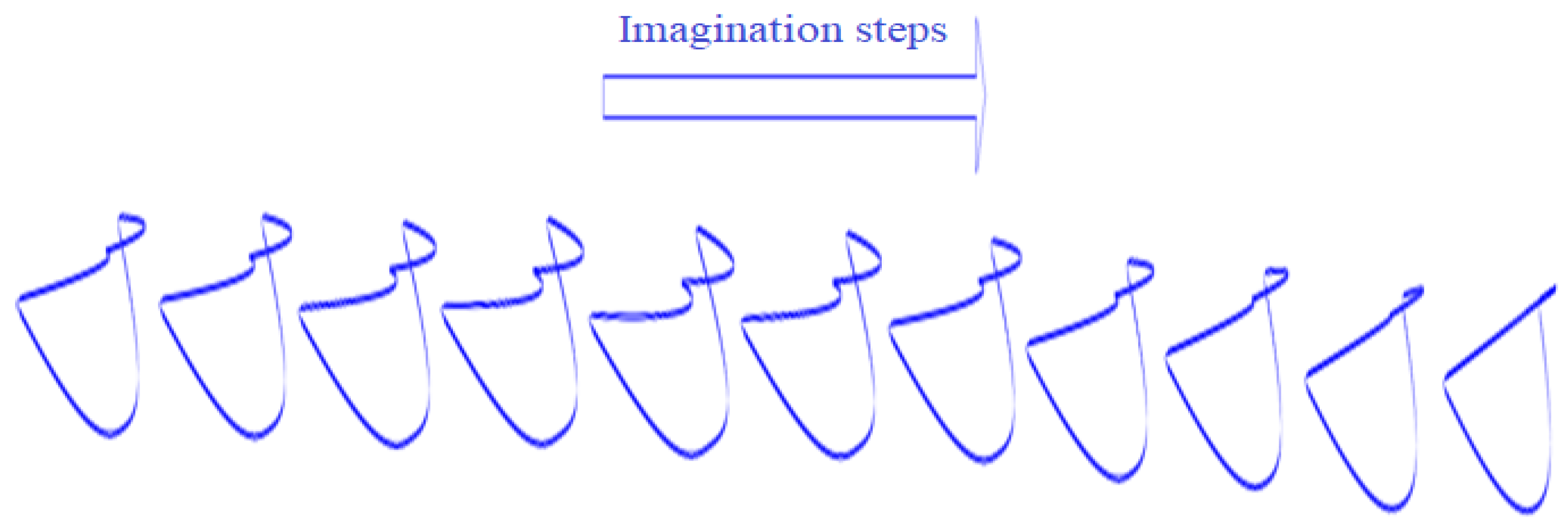
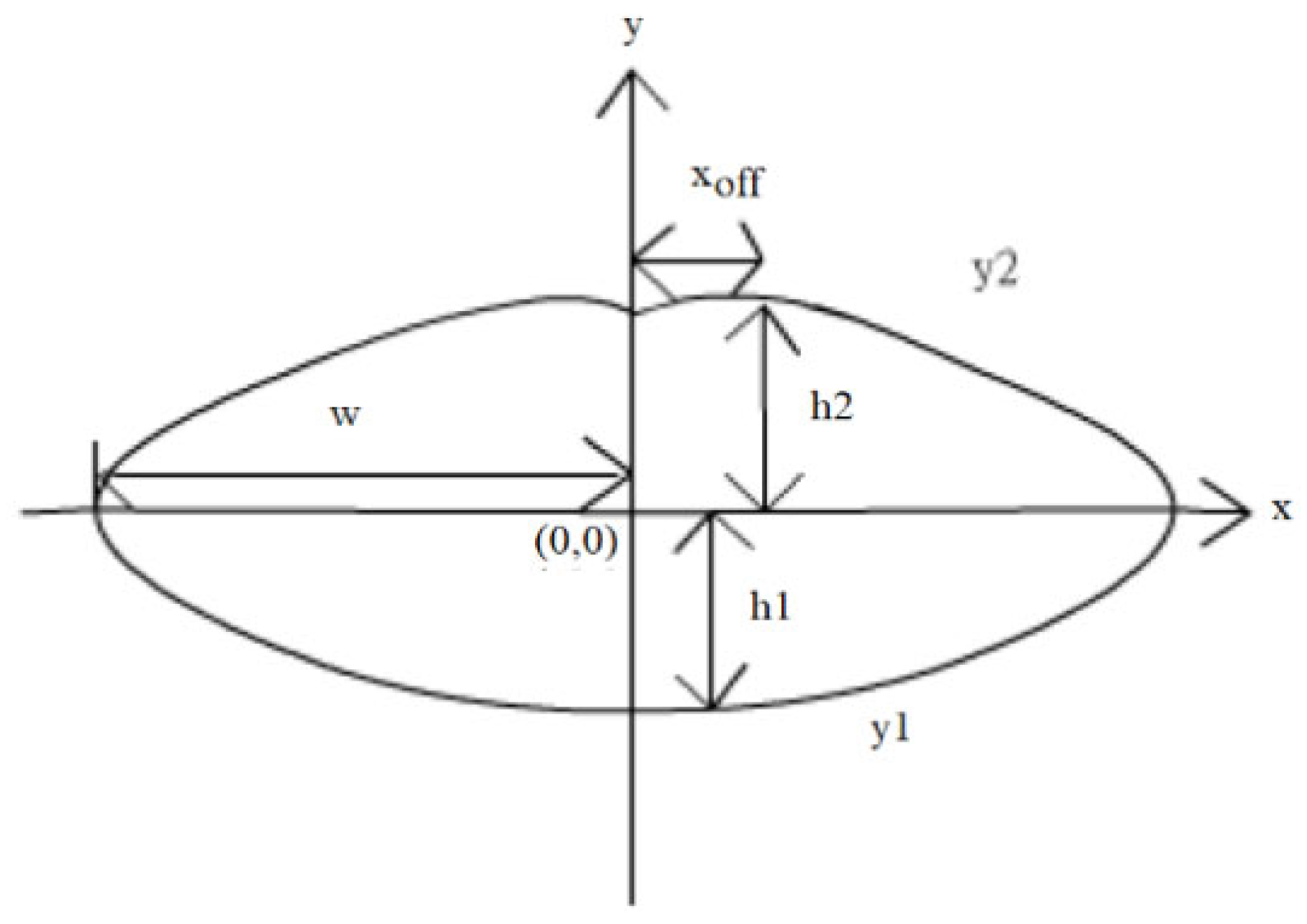
The lip-sync [71,72,73,74,75,76,77,78,79] contour formula is one of the formulas for detecting lip movements. Our model uses a lip line for the two created sounds. Figure 2, Figure 3 and Figure 4 show the steps of sound based on lip and contour synchronization. The lip images are two-dimensional (2D) and three-dimensional (3D).
The formula for the contour of the lip is:
y 1 = h 1 x s y 1 w 1 + σ 2 h 1
y 1 = h 2 w x e f f 2 x s y 2 x e f f 2 + h 2
where h1 is the height of the lower lip, h2 is the height of the upper lip, and w is half the mouth width. Xeff is the amount of curvature or the middle curve of the upper lip.

2.1.2. Collection of Signal Datasets

Three volunteers from Xian Jiaotong University collaborated with our research team by participating in a non-feedback experiment. Their ages were 30–40 years, with an average age of approximately 35 years and a standard deviation of 3 years. Our volunteers were in good health. They were trained to work mentally with their lips and to synchronize their language using videos. The experiment was conducted using a test protocol at Xi’an Jiaotong University. All volunteers signed an informed consent form for the test. It instructed the volunteers on how to think and provided other details. The participants sat in a comfortable chair in a lab, approximately 1 m in front of a 14-inch LCD monitor.

2.1.3. Filter in Frequency Domain

Our electrode cap has 32 channels in accordance with the 10–20 international system, and 16 of the 32 channels were selected. The cap was placed on the head to record EEG signals. Some studies distributed electrodes in different brain regions, such as the Broca and Wernicke areas, superior parietal lobe, and primary motor area (M1). SynAmps System 2 EEG signals were then recorded. Vertical and horizontal electrooculogram (EOG) signals were recorded using two bipolar channels to control eye movement and blinking. EEG signals were recorded after they passed through a 0.1 to 100 Hz bandwidth filter, and the sampling frequency was set to 256 Hz. Skin impedance was maintained below 5 kΩ.

2.1.4. Independent Component Analysis (ICA)

Independent component analysis (ICA) is a very broad method for EEG signal preprocessing. This is a classic and efficient way to isolate the blind source, which is the first solution to the cocktail party problem. As researchers know, a cocktail party scene generally includes music, conversation, and unrelated types of noise. Although the scene is very chaotic, because a person can see someone else communicating, they feel compelled to identify themselves and want to isolate the content of the signal source, but this scene is difficult for various reasons. Blind and source signals are mixed to create the target source signal cocktail effect. The ICA algorithm proposed for this purpose allows the computer to complete the same sound of interest. Component-independent component analysis algorithms assume that each source component is statistically independent.

2.1.5. Common Spatial Pattern (CSP)

Koles and Eta introduced a common spatial pattern (CSP) that can detect normal EEG activity. CSP attempts to find the maximum discrimination between different classes by using signal conversion to a variance matrix. EEG pattern detection was performed using the spatial information extracted with a space filter. CSP requires more electrodes to operate and does not require specific frequency bands or knowledge of these bands. CSP is also very sensitive to the positions of the electrodes and artifacts. The same electrode positions in the training process were related to memorization in order to collect similar signals. This is effective in increasing the accuracy.

2.2. New Signal Combination Model with Four Common Methods

Most researchers [15,16,17,18,80] have used a large-scale frequency domain consisting of known brain activities and noise representing unknown brain activities. A large-scale frequency filter can divide frequencies into overlapping narrow frequency filters to extract highly discriminative features [19,20]. The disadvantage of decomposing the EEG signal into narrow-pass filters is the degradation of the raw EEG signals. The essential information of each distribution event is in a large frequency band. The degradation is related to the removal of much of the EEG frequency range for processing. The main EEG signals of the events are lost. The main goal of the model is to find the most important patterns of different events in small frequency bands and to find more frequency ranges of more similar patterns. Choosing an appropriate scale for frequency filters is essential to avoid degrading raw EEG signals and to reduce noise in EEG signals. Our model reduces degradation. For collecting important distinctive patterns of brain activities, it is necessary to combine several essential small-scale frequency bands for classification. The combination of two fixed filter banks introduces new combinations of signals. These models investigate three feature extraction methods and one feature selection method.
To the best of our knowledge, at the time of writing this paper, using the combination of two fixed filter banks with a 4 Hz domain (limited frequency bands) is reported for the first time at this scale in this paper. This leads to creating new combinations of signals with 8 Hz domains in total. The performance accuracy of new signals was studied using two feature extraction methods, i.e., CSP and FBCSP, and one feature selection method, i.e., PCA. In addition to the three common methods, a Lagrangian polynomial equation was introduced to convert the data structure to a formula structure for classification. The purpose of the Lagrangian polynomial is to detect important coefficients for increasing the distinction of brain activities. It may be noted that the concept of the Lagrangian polynomial is different from auto-regression (AR), in which features are coefficients for classification.
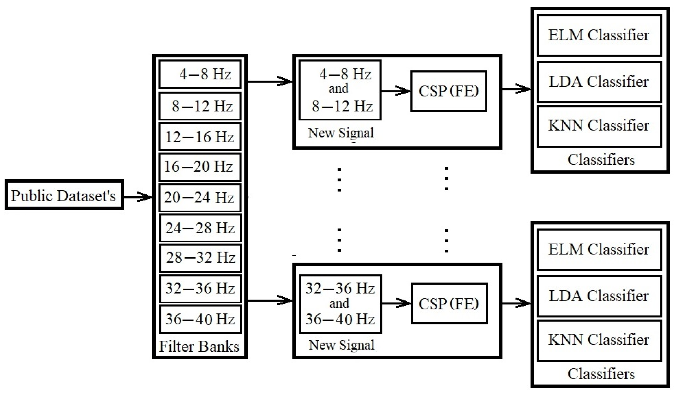
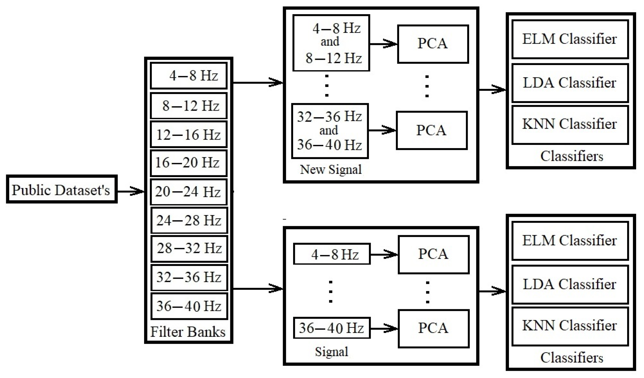
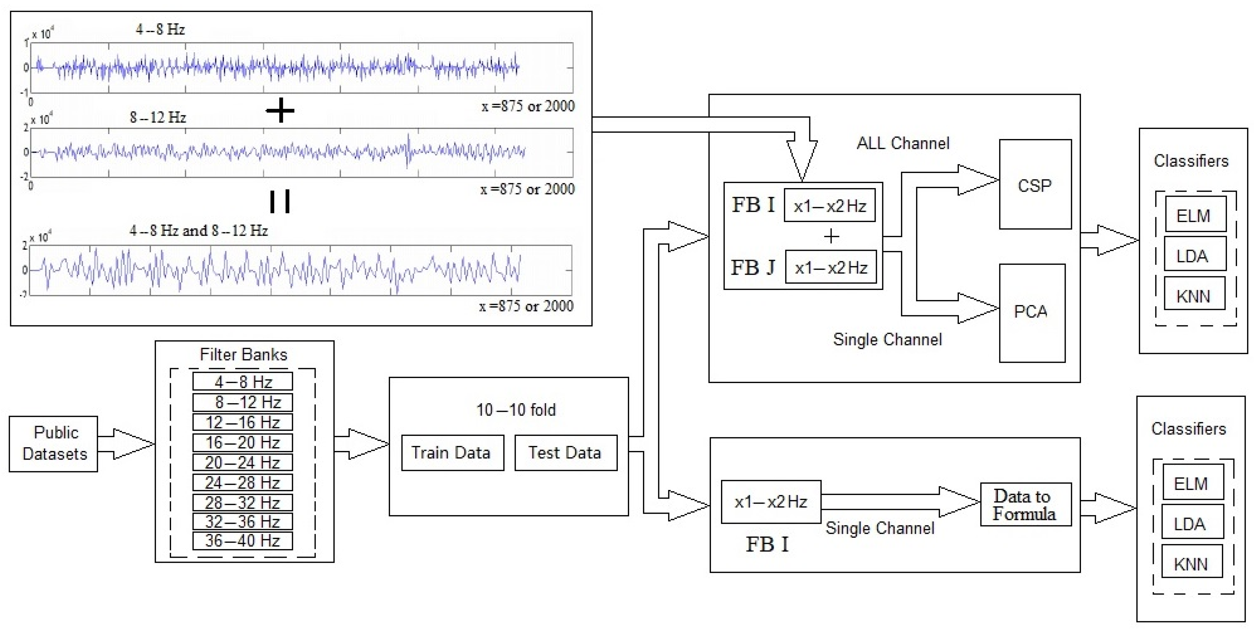
In the following subsections, we explain the details of the four main contributions of this paper by describing the models. We show an overview of the four implemented models in Figure 1, Figure 2, Figure 3 and Figure 4. Figure 5 provides an overview of the database, filter banks, and the model of the new combinations of signals with the classifiers.

2.2.1. CSP Using New Combinations of Signals

The first proposed model increases the extraction of good distinctive features from the whole channel. In this model, new combinations of signals are created and applied individually in the classification. In this case, all of the electrodes are involved in extracting features. The model consists of four phases, as presented in Figure 5 and explained below:
(1) Filtering data with Butterworth filter: In the first phase, using frequency filtering, noises and artifacts are removed with a filter bank. The domain of this filter bank is from the noise and artifact domains. EEG measurements are decomposed into nine filter banks of 4–8 Hz, 8–12 Hz, …, 36–40 Hz. All of the data are filtered by using a Butterworth filter of the 100th order. Most researchers use the Butterworth filter for filtering [20,21].
(2) Creating new combinations of signals: The combination of two fixed filter banks creates a new combination of signals. Each fixed filter bank has a 4 Hz frequency range. For example, filter bank 5 starts with 20 Hz (lower band) and ends with 24 Hz (upper band). The new signal combination of filter banks 2 and 5 supports the 8–12 Hz and 20–24 Hz frequency ranges.
The formula for new signals for all of the electrodes is calculated as:
F B i , j , m = F B i , m + F B j , m .         i , j = 1 9 ,             m = 1 n .
where FB(i,j,m) represents the ith and jth filter banks of the mth channel, and n is the maximum number of electrodes used to record the data in the dataset. Therefore, the m and i variables indicate the selected channel and the selected 4 Hz sized domain frequency (for example, m = 2 and i = 2 mean Channel 2 and the 8–12 Hz frequency range).
(3) Using CSP as the spatial filter and feature extraction: The common spatial pattern algorithm [14,15,81,82] is known as an efficient and effective EEG signal class analyzer. CSP is a feature extraction method that uses signals from several channels to maximize the differences between classes and minimize their similarities. This is accomplished by maximizing the variance of one class by minimizing the variance of another class.
The CSP calculation is performed as follows:
C = E E / t r a c e ( E E )
where C is the covariance of the normalized space of data input E, which provides raw data from a single imaging period. E is an N × T matrix, where T is the number of electrodes or channels, and N is the number of samples in the channel. The apostrophe represents the transposition operator. Trace is a set of diagonal elements of x.
The covariance matrix of both classes C1 and C2 is calculated from the average of several imaging periods of EEG data, and the covariance of the combined space Cc is calculated as follows:
C c = C 1 + C 2
C c is real and symmetric and can be defined as follows:
C c = u c λ c u c
where u c is a matrix of eigenvectors, and λ c is the diameter of the eigenvalue matrix.
p = λ 1 u c
The variances in space are equalized by u c , and all eigenvalues of p c ¯ L p are set to 1.
S L = p c ¯ L p
S R = p c ¯ R p
S L and S R are common special sharers, provided that S L = B λ L B and S R = B λ R B and λ L + λ R = I .
Eigenvalues are arranged in descending order. And the projection matrix W is defined as follows:
W = U T P
where U T and P are the transfer matrix and data.
The reflection matrix of each training process is as follows:
Z = W × i
where N rows are selected to represent each period of conception W P ( p = 1,2 , , N ) , and the covariance P of Z and P components of the feature vectors are calculated for the nth instruction.
The normalized variance used in the algorithm is as follows:
f p = log 10 V a r ( Z p ) / V a r ( Z p )
(4) Performing classification using classifiers: Classification is performed using three classifiers in our model: LDA with a linear model, ELM with the sigmoid function using 20 nodes, and KNN with five neighborhoods (k = 5).
Two public datasets were selected according to details described in the next section. After filtering the data, the combinations of two filter banks based on Formula (3) for all of the electrodes are created. Each combination of the two filter banks is considered separately in the next steps. In the next step, CSP is applied for spatial filtering, the removal of artifacts, and the extraction of features from the new combination of signals. The experimental model of training data and test data is presented in Section 3.

2.2.2. FBCSP [82,83,84] Using New Combinations of Signals

The second proposed model increases the good distinctive features extracted from the whole channel, which has the additional step of feature selection compared to the first model. In this model, new combinations of signals are created, and the best signals from both primary and new signals are selected using feature selection and used for classification. All of the electrodes cooperate for noise and artifact filtering and the extraction of features. This model consists of the following phases, presented in Figure 6 and explained below:
(1) Filtering data with Butterworth filter: This step is the same as the first step in the previous section, i.e., Section 2.2.1.
(2) Creating new combinations of signals: This step is the same as the second step in the previous section, i.e., Section 2.2.1.
(3) Applying CSP as the spatial filter and performing feature extraction: In this phase, the CSP algorithm extracts m pairs of CSP features from new combinations of signals. This is performed through spatial filtering by linearly transforming the EEG data. Then, the features of all new signals are collected in a feature vector for the ith trial, i.e.,
X i = c f 1 , c f 2 , , c f 9
where c f b R 2 m denotes m pairs of CSP features for the bth band-pass-filtered EEG measurement, X i R 1 × ( 9 2 m ) .
(4) Collecting and selecting features: In this phase, an algorithm called Mutual Information Best Individual Features (MIBIF) is used for feature selection from the extracted features, and it selects the best features, which are sorted (in descending order) using class labels.
In general, the purpose of the mutual information index in MIBIF [85,86] is to obtain maximum accuracy with k features selected from a subset of S F , in which the primary set F includes d features. This approach maximizes the mutual information I(S; Ω). In the classification of features, input features, i.e., X, are usually continuous variables, and the Omega class (Ω) has discrete values. So, the mutual information between the input features X and class Ω is calculated as:
I X ; Ω = H Ω H Y Ω
where ω Ω = { 1 , . . , N ω }
And the conditional entropy is calculated as:
H Ω X = X ω = 1 N ω p ω X l o g 2 p ω X d x ,
where the number of classes is Nω.
In general, there are two types of feature extraction approaches in the mutual information technique, namely, the wrapper and filter approaches.
With the wrapper feature selection approach, the conditional entropy in (14) is simply:
H Ω X = ω = 1 N ω       p ω X l o g 2 p ω X ,
P(ω|X) can be easily estimated from data samples that are classified as class ω using the classifier over the total sample set.
Mutual information based on the filter approach is described briefly in three steps:
Step 1: Initialize set d feature F = f 1 , f 2 , , f d and select feature set S = Null.
Step 2: Compute MI features based on I( f i |Ω) for each i = 1…d, where f i belongs to F.
Step 3: Select the k best features that maximize I( f i |Ω) [84,85].
Step 4: Repeat the previous steps until S = k .
(5) Performing classification using classifiers: This step is the same as the fourth step in the previous section, i.e., Section 2.2.1.
This model was applied to one public dataset (including left hand and right hand), which is described in the next section. Most of the steps in the two models are the same. The exception is that one phase of feature selection is added between CSP and the classifiers, which selects the best features by applying mutual information feature selection after collecting the extracted features of new combinations of signals. About 10 to 100 features are selected and sent to the classifiers for classification.

2.2.3. Lagrangian Polynomial Equation Using New Combinations of Signals

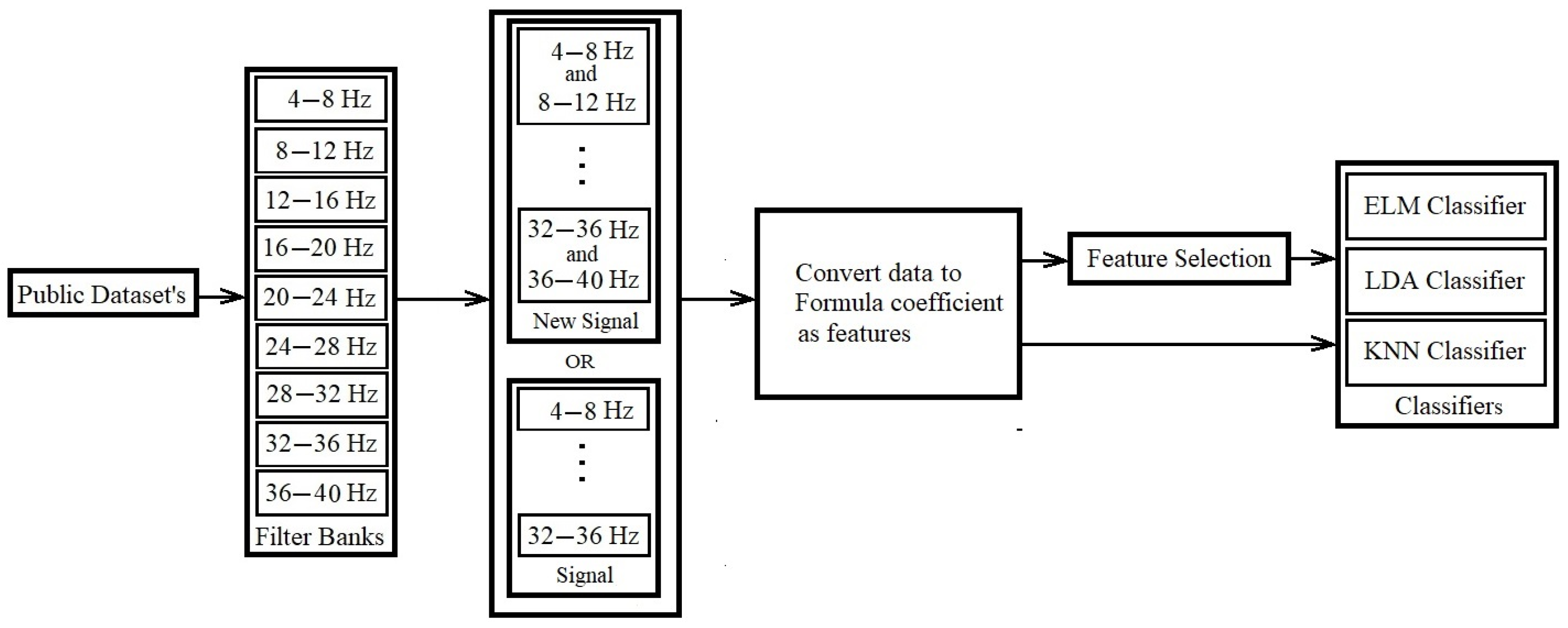
The third proposed model increases the number of good distinctive features extracted from every single channel separately. In this model, we use a Lagrangian polynomial model to transform the data into formulas, which are then used as features for classification. A single channel/electrode is involved in the extraction of features and classification, as illustrated in Figure 7 and explained in the following steps.
(1) Filtering data with Butterworth filter: In the first phase, using frequency filtering, the noise and artifacts are removed with a filter bank. This process is the same as the first step in Section 2.2.1, with the difference being that it involves single channels individually.
(2) Using filter bank (sub-band) signals or new combinations of signals: Two models are considered input data, including sub-bands in the names of filter banks and new combinations of signals. New combinations of signals are created based on the following formula for a single electrode. This formula is used for the calculation of a single electrode or channel.
S _ F B i , j = S _ F B i + S _ F B j .       i , j = 1 9 .
where S _ F B i , j represents the filter bank signal.
(3) Converting data to a formula of coefficients with different orders by using the Lagrangian polynomial equation: The input data are about 1 s from 3.5 s of imagination time. The Lagrangian polynomial equation converts these input data of the two single channels to coefficients for classification.
The Lagrangian polynomial is described below.
There are k + 1 data assets x 0 , y 0 , , x j , y j , , x k , y k , while each x j is unique. The interpolation polynomial, as a linear combination, is in the Lagrange [87,88] form.
L x = j = 0 k y j l j ( x )
The structure of the Lagrangian polynomial is described in the form of:
l j x = 0 m k x x m x j x m = x x 0 x j x 0 x x j 1 x j x j 1 x x j + 1 x j x j + 1 x x k x j x k
where 0 j k . In fact, in the initial assumption, two x j are not the same, and then (when m j ) x j x m 0 ; therefore, this expression is the appropriate definition. The reason is that pairing x i = x j with y i y j is not allowed, so no interpolation function L such that y i = L ( x i ) can exist, and the function gives a unique value for each argument x i . On the other hand, if y i = y j , then x i = x j have the same value as one single point. For all i j , l i ( x ) includes the term x x i in the numerator, so with x = x i , the whole product will be zero, and l i x is:
j i : l j x i = m j x i x m x j x m = x i x 0 x j x 0 x i x 1 x j x 1 x i x k x j x k = 0
On the other hand,
l j x i = m j x i x m x j x m = 1
In other words, the Lagrangian polynomials are l j x i = 0 at x = x i . Unless it is l j x i = 1 with the lack of the x x j = 0 term, it follows that y j l j x i = y j , so at each point x j , L x j = y j + 0 + 0 + + 0 = y j , which shows that L interpolates the function entirely.
The final formula is:
l x = a n x n + a n 1 x n 1 + + a 1 x + a
where a n , a n 1 ,…, a 1 , a are coefficients of the Lagrangian polynomial, and n, n − 1, n − 2, …, 1 are the orders.
(4) Classifying with/without feature selection methods: First, all features are used for the classification. Second, the best equation coefficients are selected using feature selection for the classification.
(5) Performing classification using classifiers: In this phase, we perform classification based on features to determine accuracy using classifiers. This phase is similar to the last phase of the two above models.
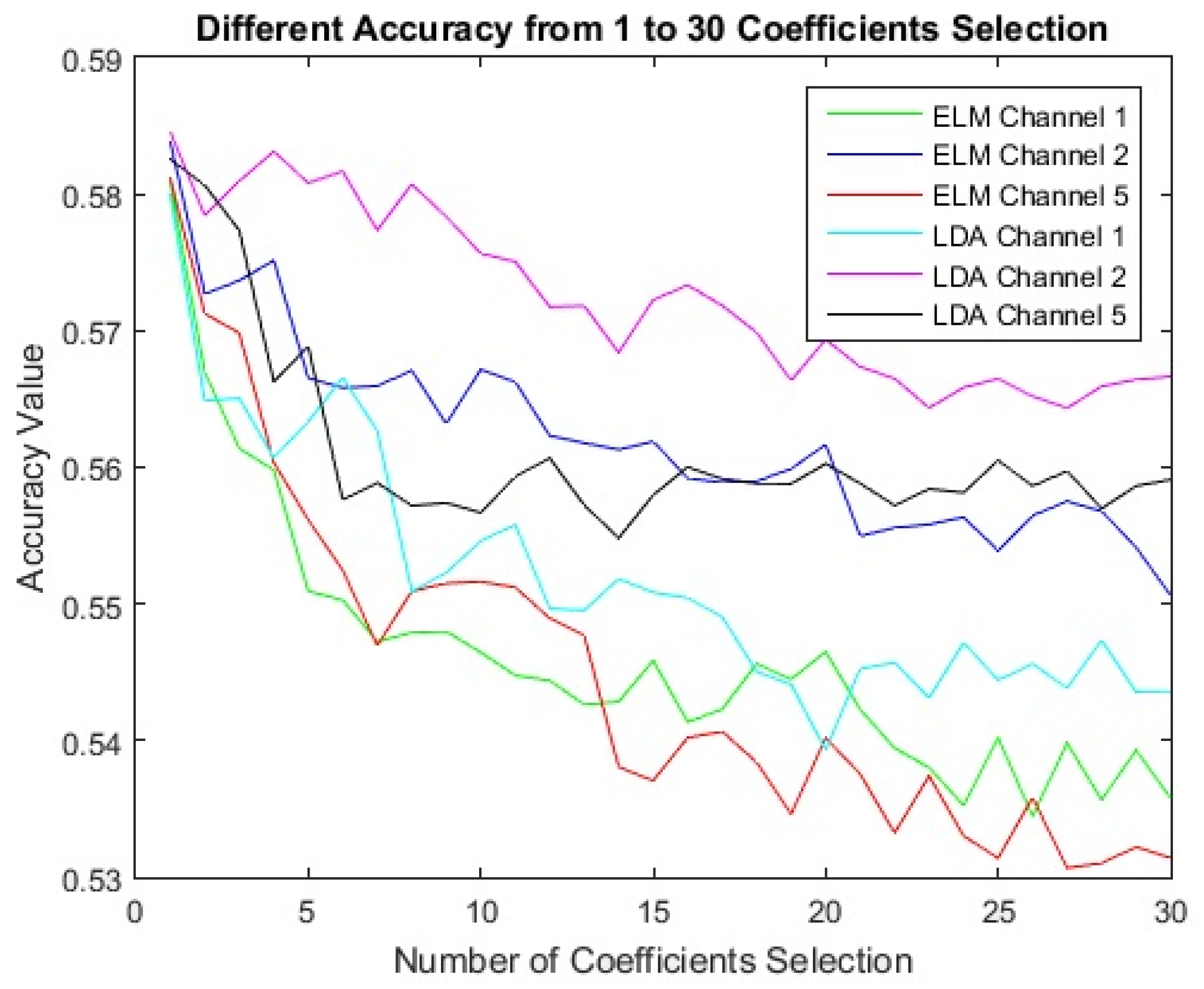
This model was tested on one public dataset (including left and right hands) for examination. We describe this public dataset in more detail in the next section. Single channels are applied for processing. Then, the combination of two filter banks based on Formula (17) for single electrodes/channels is calculated. Each combination is considered separately in the next steps. In the next step, two procedures are considered for processing. The first procedure uses fixed filter banks of a single channel, and the second procedure uses the new combinations of signals for a single channel. Then, each procedure uses the Lagrangian polynomial equation to convert data to formula structures. The Lagrangian coefficients are considered features for the classification. Feature selection is not used in the first procedure, but it is used in the second procedure. Mutual information feature selection selects the best features from 1 to 30 features. And finally, the coefficients selected as the most effective features are sent to the LDA, KNN, and ELM classifiers for classification.

2.2.4. PCA Using New Combinations of Signals

The fourth proposed model increases the good distinctive features extracted separately from single channels. In this model, using PCA, we sort the data without dimensional reduction based on the best features before the classification. A single electrode is used for sorting the features and transforming data to a new space, followed by classification, as illustrated in Figure 8 and explained in the following steps:
Filtering data with Butterworth filter: The first phase is the same as the first phase of the previous model.
Using filter bank (sub-band) signals or new combinations of signals: The second phase is the same as the second phase of the previous model.
Sorting features by PCA: The purpose of PCA, as an orthogonal linear transformation method, is to reduce the dimensionality by transferring data to a new space and sorting them. The greatest variance lies on the first coordinate as the first principal component, the second-greatest variance is on the second coordinate, and so on. PCA is introduced as one method for reducing primary features using the artificial transformation of data to a new space [89,90,91,92].
The basic description of the PCA approach is as follows. Let us define a data matrix X M × N , where M is the number of observations, and N is the number of features. Then, C N × N is defined as the covariance matrix of matrix X :
C = V a r ( X 1 ) C o v ( X 1 , X 2 ) C o v ( X 1 , X N ) C o v ( X 2 , X 1 ) V a r X 2 C o v ( X 2 , X N ) C o v ( X N , X 1 ) C o v ( X N , X 2 ) V a r ( X N )
where C o v X i , X j = 1 M 1 M X i k X ¯ i X j k X ¯ j , and v a r X i = σ X i 2 .
Eigenvectors and the eigenvalue matrix are produced by matrix C :
C Γ = Λ Γ C = Γ Λ Γ
where Λ N × N is a matrix of sorted eigenvalues λ 1 λ 2 λ N :
Λ = λ 1 0 0 0 λ 2 0 0 0 λ N
And Γ N × N is a matrix of eigenvectors (each column corresponds to one eigenvalue from matrix Λ ):
Γ = γ 11 γ 12 γ 1 N γ 21 γ 22 γ 2 N γ N 1 γ N 2 γ N N
Finally, the matrix of principal components is defined as:
Y = Χ Γ = y 11 y 12 y 1 N y 21 y 22 y 2 N y N 1 y N 2 y N N
Each of the N features x 1 , x 2 , , x n can be explained with parameters from matrix Y as a linear combination of the first K principal components: x m n = k = 1 K γ n k y n k .
Performing classification using classifiers: The fourth phase is the same as the fourth phase of the previous model, with differences in the scale of input data.
This model uses the entire 3.5 s as input with the PCA method. PCA is used for transferring data and sorting in our research.
Finally, we present the combination of filter banks in Figure 9.

2.3. New Linear and Nonlinear Bond Graph Classifiers

The bond graph classifier uses the distance calculation method for classification. This model is local, and the focus is on its structure. The boundary uses central point data. Our model has different steps: (1) Search for the minimum path between nodes (attributes). (2) Create the center of the arc with the node and longest sub-nodes. (3) Calculate the boundary between the two centers. (4) Create the main structure to support all borders. In this section, we begin with a brief description of the proposed classifier model in the main structure. Our method is as follows.
Our method uses one of the greedy algorithms (Prim algorithm) to find the minimum spanning tree, which is weighted based on a directionless diagram. A subset of edges is provided by the Prim algorithm to minimize the total weight of all of the tree edges. The algorithm arbitrarily starts the tree from one vertex and proceeds to another vertex once. It then adds the cheapest possible connection from the tree to the other vertex. Following the development of the algorithm in 1930 by the Czech mathematician Vojtěch Jarník, the algorithm was republished by computer scientists Robert C. Prim in 1957 and Edsger W. Dijkstra in 1959. These algorithms find at least one spanning diagram in a potentially truncated router. The most basic form of the Prim algorithm finds only minimum spanning trees in connected diagrams. In terms of asymptotic time complexity, these three algorithms are equally fast but slower than the more complex algorithms. However, for graphs that are sufficiently dense, the Prim algorithm can run in linear time, matching or improving on the time limits of other algorithms [93,94,95,96,97] (Figure 10).
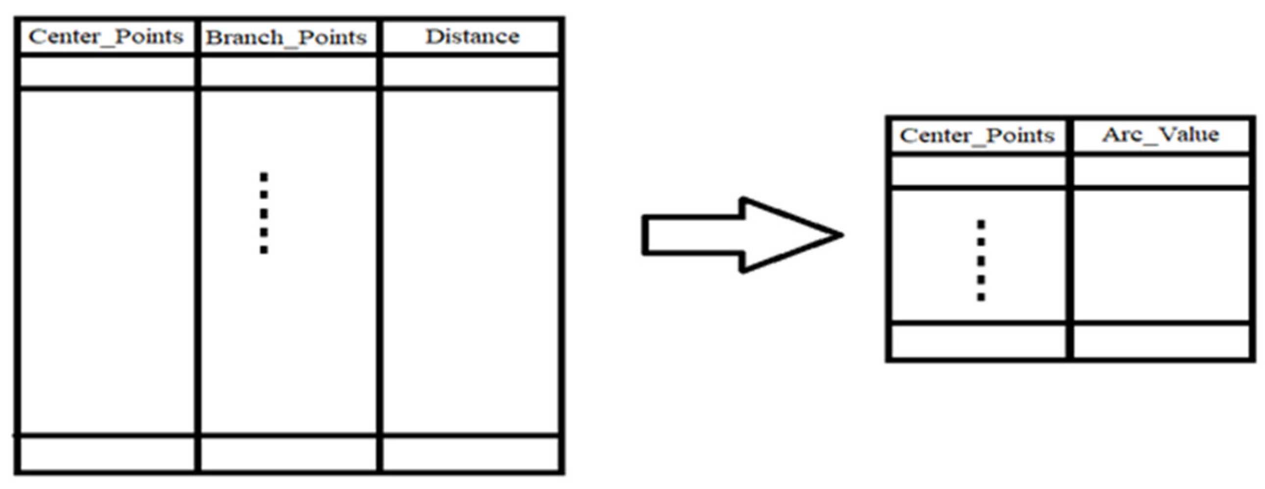
This tree matrix contains the nodes above and below the nodes. Each head node determines the smallest distance from its sub-nodes. They then created a slightly larger arc than the longest arc (28).
Distance_Arc = longest sub-nodes + alpha × longest sub-nodes
All head nodes of different classes have arcs for participation. Our model has three modes to detect boundary points: (1) Near the center, border points can be recognized. (2) The local center can detect the boundary point. (3) Near the center of the node, the boundary point can be detected.
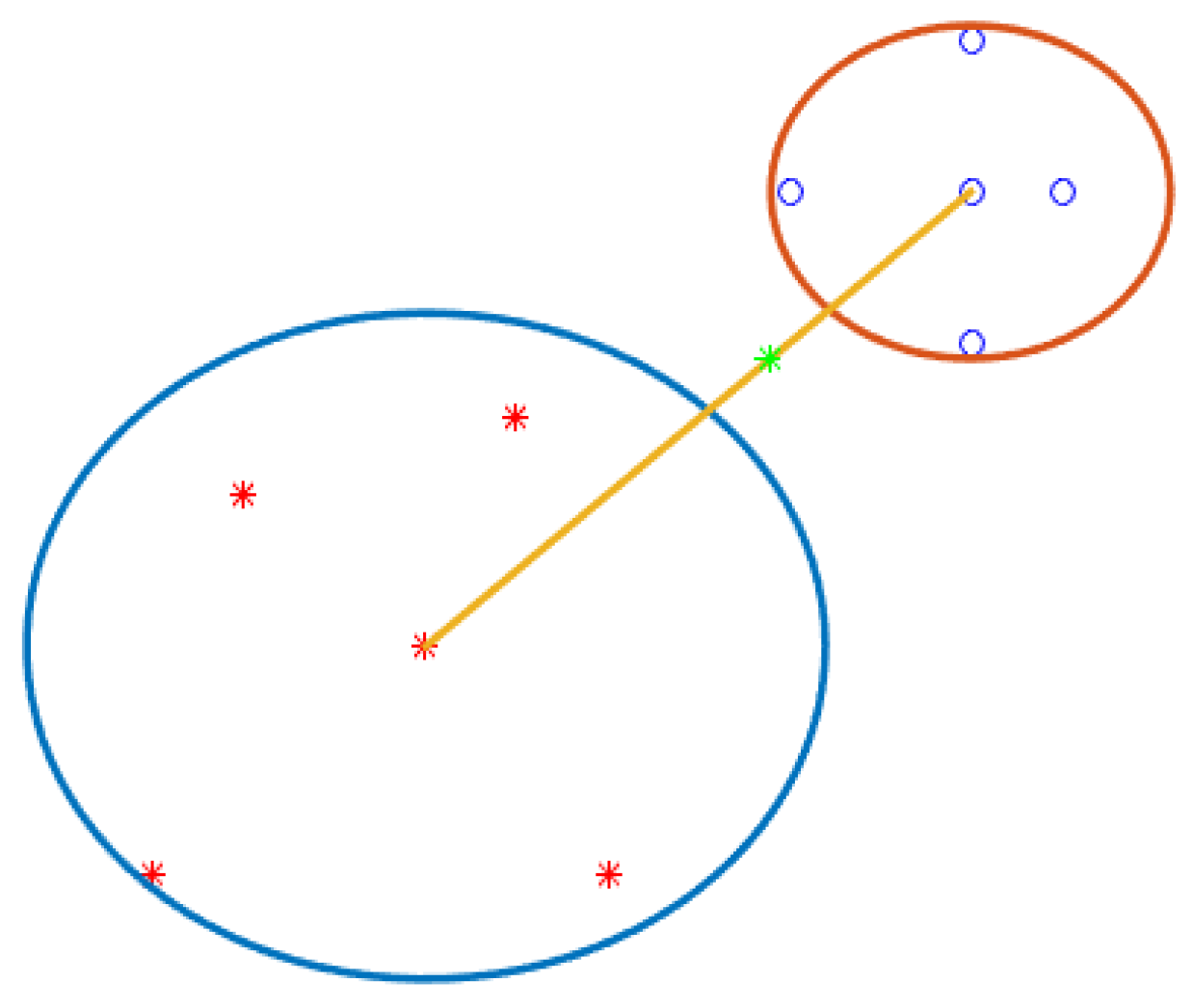
In one case, the first case, the boundary point of the arcs can be found when the arcs from two different classes do not intersect each other. Therefore, the distance between two central classes is calculated. And a point between two separate arcs is defined as a border.
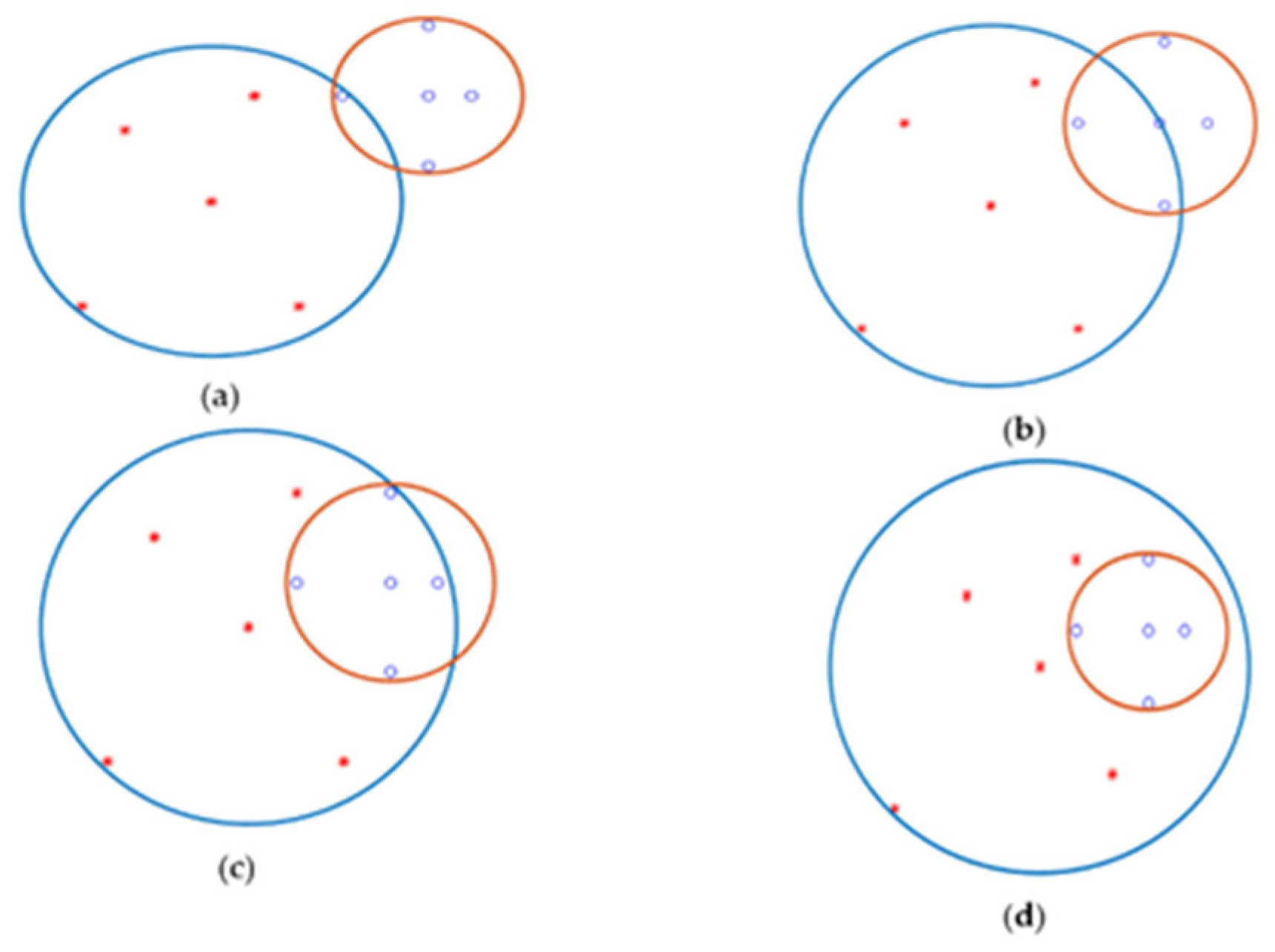
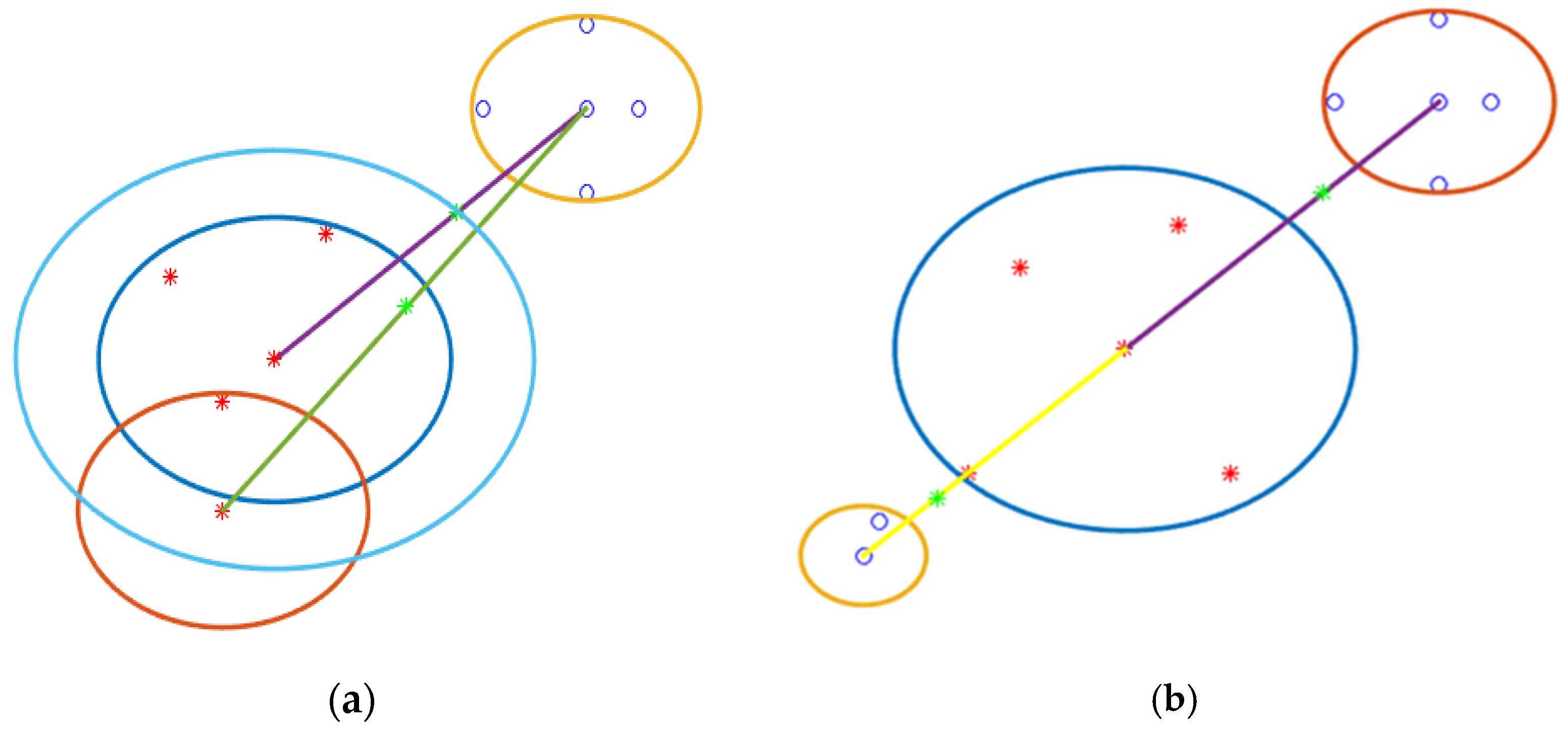
Figure 11 shows two different class centers. The blue and red dots belong to classes one and two. The two centers are connected by a yellow line (the yellow line is the distance between the two centers). The red arc of class one and the blue arc of class two do not intersect each other, and the border points with green points are located in the middle of the two arcs. Other states of the arc have intersections, in which case the arc must break and turn into small arcs, because this method does not recognize the boundary points like the first case. This state occurs when more nodes are distributed on the border. The main question is which arc should be broken? In Figure 12, there are four modes in this situation. In all of them, it was necessary to break the blue arc into two small arcs.
After finding all border points, some border points were not necessary. Therefore, they had to be removed because some points support all points. In Figure 13, the two-class arcs and one-class arc have two boundary points. One part of the program recognizes that some arcs are necessary to keep and others must be deleted because one boundary point also supports another boundary point. One green border point on the blue arc is light, and the other is the arc. This implies that when two boundary points are in one direction, one supports the other. In Figure 13, the two different directional boundaries and locations do not remove another boundary point. It might be assumed that if another green dot in the blue–green dot arc is bright, another green dot should be removed. It is essential for boundaries to remove some boundary points, where only a class one arc has some boundary points with different class-two arcs. Class two is the same as class one. Our model stores tree data, such as a matrix, to determine the longest arc. Then, another table is created. Since arcs and centers work together to find the boundary when it is about to break, the first table must be returned to create two others (Figure 14).
First, we briefly explain the pseudo-code of this model. In the second step, the flow diagram clearly shows the model details.
(1) Data collection: Data are collected from each field (collection of signal data from different areas and EEG signals (brain signals)).
(2) Data input of model: Two models are considered for performing the classification. (1) Raw data are sent to a classifier directly. (2) Data processing is performed by filtering the raw data sent to a classifier for classification (extracting new features from raw data).
(3) Classification models: Two models are used for classification. (1) In the first model, the data include training and testing data. That is, the data are divided into two parts. (2) In the K-fold model, the data are divided into K parts. One part is considered for testing and the rest is used for training. All parts are used once for testing.
(4) Class selection model: One of the classes is selected as the first class, and one of the other classes is selected as the second class.
(5) Minimum routing algorithms: Minimum routing is found for each class separately. All vectors of each class are passed to the Prim algorithm function. But in the first model, we use the Prim algorithm. Each vector is considered a node that contains all vector information.
The outputs of a connection matrix are the nodes with the minimum routing; the first column is the number of nodes, and the second column is the number of neighbors, which includes the minimum routing. No leaves are observed in the first column. These only exist in the second column. The original algorithm uses the Euclidean distance to calculate. This table is arranged for further processing.
(6) Creation of an arc: Based on the matrix, this function creates an arc based on two models. (1) An arc is created from the head node in such a way that it includes all the children, so the children themselves are the head nodes for other nodes (children). (2) An arc is created for the head node so that it includes all children, and the children of the hip node have no children. The distance of the arcs is the maximum distance between the head node and the child node plus the epsilon value.
(7) Identification of centers and calculation of boundary points (function): This function finds boundary points using the centers and arcs of two classes. Finding the boundary points involves three possible modes, which are briefly described in this section. These modes are:
(7.1) No contact between arcs that are far from each other: The border point is in the middle of the distance between two arcs of two nodes of two different classes. In other words, they do not interrupt each other. This can be seen in Figure 11. The Euclidean distance between the two is
Euclidean Distance = the size of the center arc (Class 1) + the size of the second center arc (Class 2) + the outer distance between the two arches
(7.2) No contact between an arc and an arc inside another arc: Two arcs from two nodes of two different classes intersect and are in contact. The smaller arc remains, and the larger arc is broken into smaller nodes with smaller arcs; each node becomes an arc node, and model 7.1 or 7.3 is used to find the boundary (Figure 12).
(7.3) Contact between arcs: The border between arcs is determined based on a criterion. This can be seen in Figure 12 and Figure 13.

2.4. Deep Formula Detection with Formula-Extracting Classifiers

2.4.1. Classification of Deep Formula Coefficients by Formula-Extracting Coefficients in Different Layers along with Prevalent Classifiers

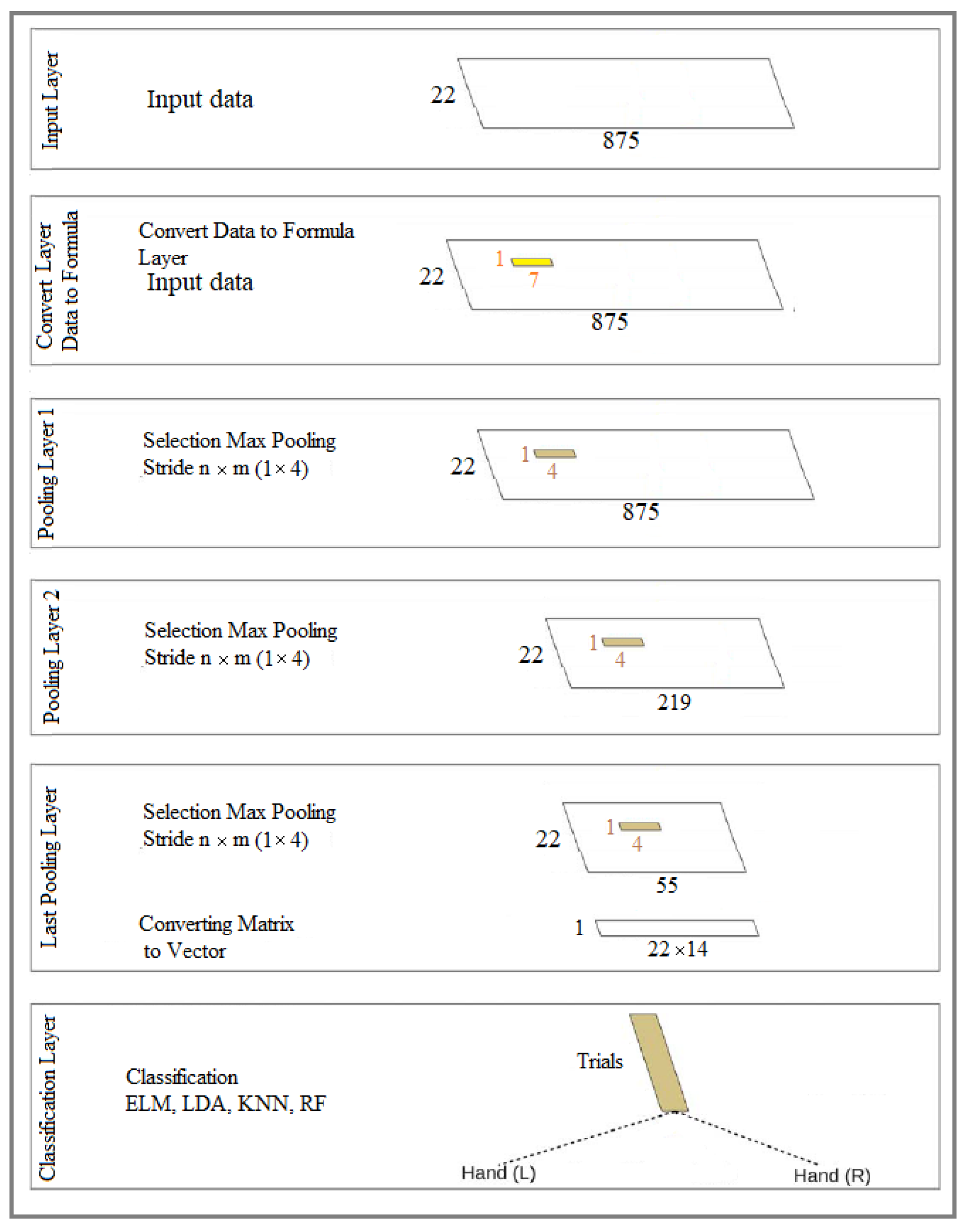
This section introduces a new model for deep detection instead of deep learning. In this way, the data in the first layer are converted into a formula (formula coefficients with orders), and then the effective coefficients of the formula are selected from other layers based on the coefficient selection function. After the last layer, the coefficients selected as coefficients from the original formula are sent to different classifiers as training and test data. This model includes the following steps (Figure 6):
(1) The input layer as a data-to-formula conversion layer: This layer is a data-to-formula coefficient conversion layer. First, windows with specific sizes are defined to convert data into formula coefficients, and the conversion is complete. In other words, the data are transformed into a polynomial equation using the Lagrange formula based on the defined window size (filter in deep learning). In this model, overlapping is omitted. The jump size is selected as the window size. In this layer, the entire matrix or vector is converted into a formula.
(2) The effective coefficient selection layers of the formula: These layers are similar to convolution neural network (CNN) layers, but with the difference that new features are extracted in the CNN layers, but noise is removed from the formula coefficients in these layers. In our first implementation, only sampling layers (similar to CNN sampling layers) are used. No noise removal layer is applied. In other words, the sampling function is used in each layer. These functions are applied based on specific criteria so that the most effective coefficients of the formula are selected and the ineffective coefficients of the formula are removed. These effective coefficients are related to the separation formula (difference formula coefficients) for two classes. This model was implemented as a prototype in our research.
(3) Common classifiers for data: In this section, several common classifiers, namely, RF, KNN, SVM, and LDA, are used.

2.4.2. Detecting the Range of Deep Formula Roots by Extracting Coefficients of Formulas in Different Layers along with the Extraction of the Root Ranges Together with the Classifiers of Event Formula Roots

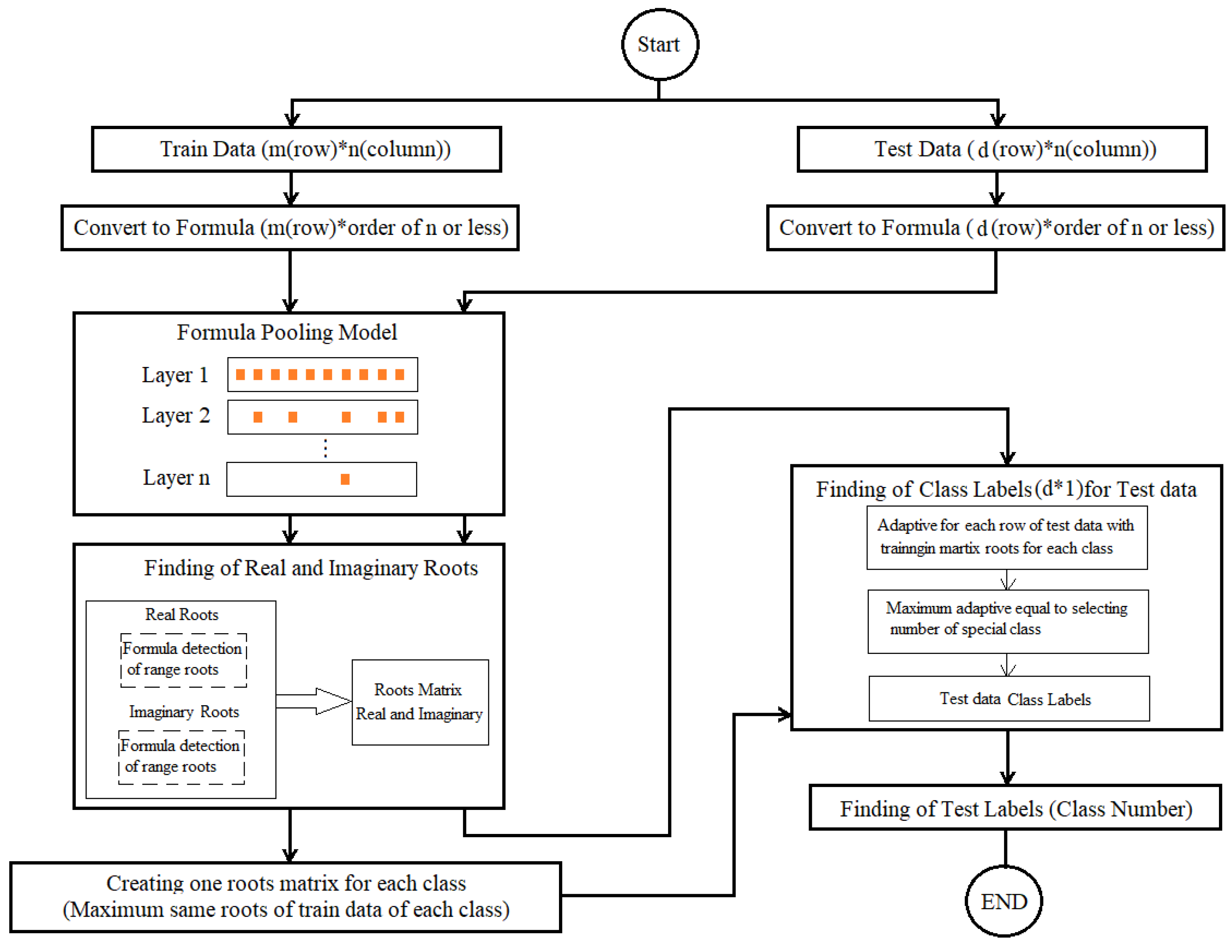
This section introduces a new model for deep detection instead of deep learning. In this way, the data in the first layer are converted into a formula (formula coefficients with orders), and then the effective coefficients in the formula are selected in other layers based on the coefficient selection function. After the last layer, the selected coefficients are selected as coefficients from the original formula to select the root of the difference formula in an interval. The interval of the roots is determined for the next step based on the selected coefficient. This model includes the following steps (Figure 15):
(1) Input layer as a data-to-formula conversion layer: This layer is the same as that described in the first part of Section 2.4.1, with the difference that the window selection function can be different.
(2) Layers for selection of the effective coefficient of the formula: These layers are the same as those described in the second part of Section 2.4.1, with the difference that the selection function of the coefficients can be different in the layers.
(3) New classifier based on root (root ranges of formulas) formulas for classes: A new classifier is introduced to extract and identify the roots of group members as a class, so the roots of a class are introduced based on the common roots of the majority of members of the same class. In this way, the roots (range of roots) of the members of each class are identified during learning. A test member is assigned to a class that has a very high similarity between the roots of that member and one of the classes. Our test was run on members of two classes.
Since finding the exact location of the roots takes a lot of time, we chose the method of finding the roots of equations or polynomials in specific time intervals, which requires less time. That is, instead of finding the exact root, we determine the root interval. However, the roots can be discovered in certain fixed and bounded intervals, where the root exists in this interval.
In the following, we describe the new root extraction and detection classifiers in more detail.
Suppose that the function is given by the table in the figure below so that we have i j : x i x j .
In this method, we assume that each L 0 x , L 1 x , , L n x is a polynomial of degree n.
P x = L 0 x f 0 + L 1 x f 1 + + L n x f n
where we have n for j = 0,1 , , n .
L j x = ( x x 0 x x 1 x x j 1 x x j + 1 ) x x n ) ( x j x 0 x j x 1 x j x j 1 x j x j + 1 ) x j x n )
We have
L i x i = 0 ,   i = j 1 , i < > j L i x i = 0 ,   i = j 1 , i < > j
So, we will have
P x i = f i ,           i , 0,1 , , n .
That is, the polynomial (x) P defined by (1) holds in the condition P x i = f i .
The model for finding roots in a range is based on dividing the equation into certain intervals. The range that meets the condition of having a root is known as the root range, which must have the following conditions.
The following equation is used for real roots.
O 1 . . m = a n x n + a n 1 x n 1 + + a 1 x 1 + a 0 x + b 1 . . m .       i , j , n = 1 m .
The following equation is used for imaginary roots.
O 1 . . m = a n x n + a n 1 x n 1 + + a 1 x 1 + a 0 x f + b 1 . . m .         i , j , n = 1 m , f = 2,4 , , d
We use the following method to establish the condition of the existence of the root in the specified interval.
If O i = O n and O n = O j , and ( O i is positive and O j is negative) or ( O i is negative and O j is positive), i < n < j leads to one root and is an n value range.

2.4.3. Dataset and Experiments

Dataset IIa [98] from BCI Competition IV was used and is described in Section 3.1. For our research, 10-10-fold cross-validation was used for experiments. This dataset was used for all four methods.
This structure makes it easier to find the roots of the equation or polynomial in specific intervals. This means that it does not find the exact positions of roots; it finds roots in fixed, limited, specific intervals, and the currently commonly used classifiers use different formulas to differentiate the extracted class property.
When the coefficients of the formulas are entered into the classifier, the coefficients of the training and test formulas are separated using a specified function. This method was also executed using the K-fold 10-10 method.
The root classifier section introduces the roots of a class based on the common roots of the majority of members of the same class. In this way, the roots (range of roots) of the members of each class are identified during learning. Each test member belongs to a class where there is a lot of similarity between the roots of that member and one of the classes.
This section describes the values assigned to the variables and structures for practical implementation. This includes the following conditions:
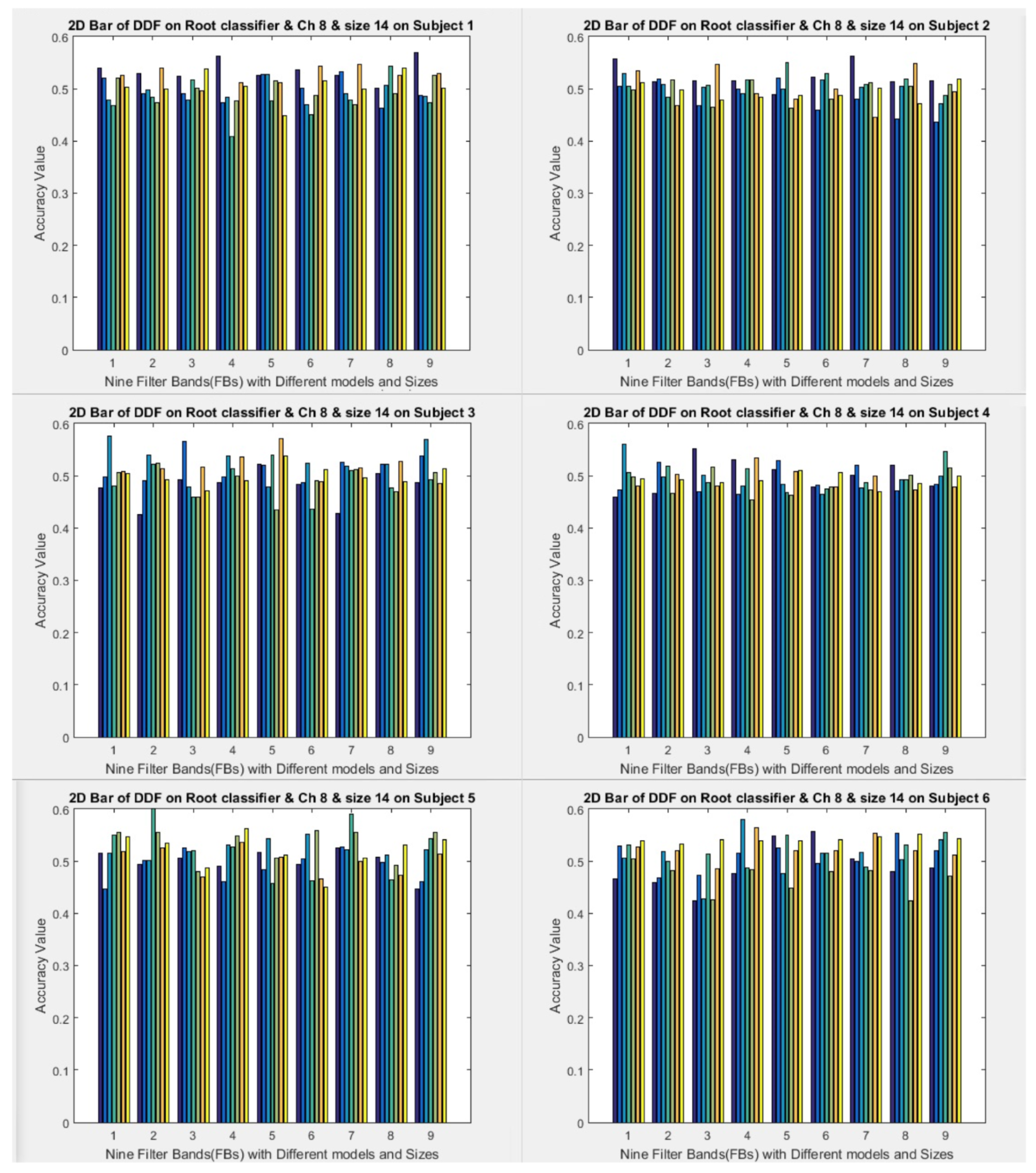
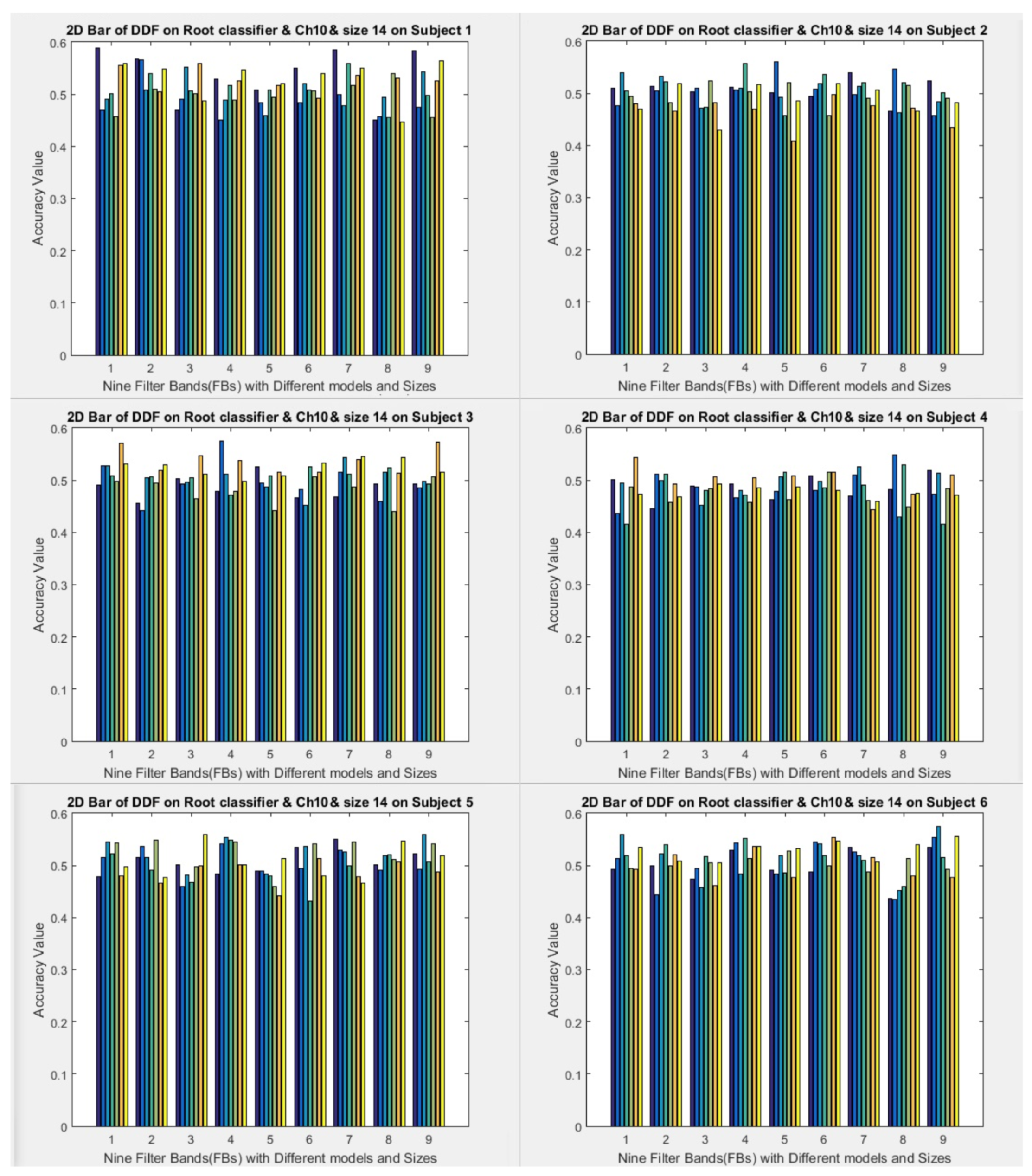
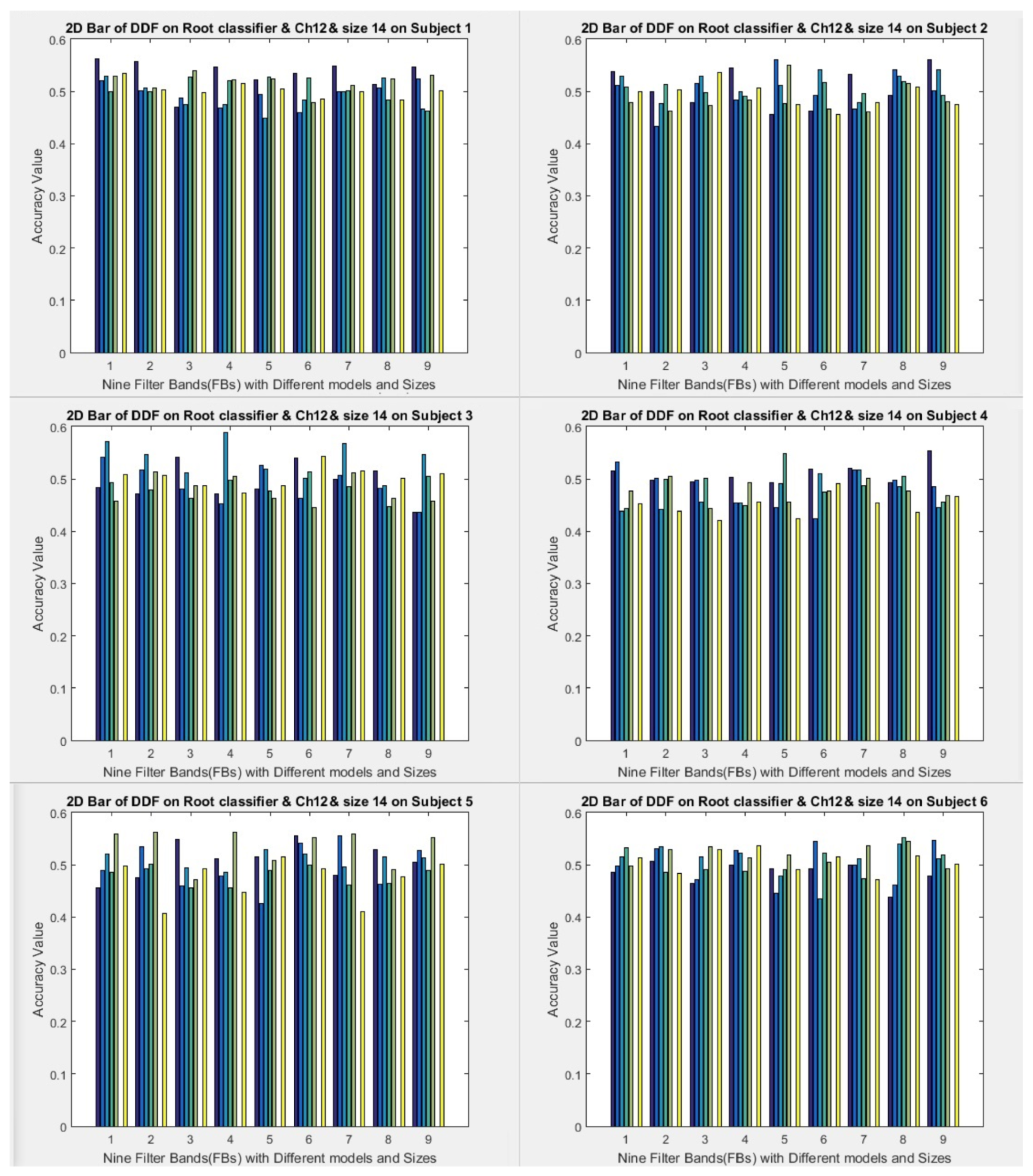
(1) All filter banks (1–9) with three selected channels (8, 10, and 12) were used to run the models.
(2) Two fixed window sizes (7 and 14) were used to convert the data into formulas in the first layer.
(3) A window sampling size was used for the second and subsequent layers, 3, 5, 7, 10, and 15, using a size of 7 (data-to-formula conversion). The window sampling sizes for the second and subsequent layers were 5, 10, and 14, using a size of 14 (data-to-formula conversion), and various variables were used for investigation. The results for the two cases mentioned above were obtained. However, this study presents a formula with a window size of 14.
(4) The root folder had ten folders and ten executions. An average of all of the results of the 10 folders after execution was considered the final result. Therefore, it was executed ten times, and the average of the ten times was considered the final result. For the classifier, we set the root range (spin range) to 0.5 and set it between 0.001 and 1. However, the smaller the interval between these roots, the more time it takes to find the formula roots (our model considers only one mode).
Next, an overview of the proposed new model is provided with prevalent classifiers in Figure 16.
The sizes of the output layers and filters are used in four ways:
(1) In all models, the input layer includes 288 mental images, 9 filter banks, 22 channels, and 875 features for each channel during mental imagination for each brain activity on the left or right. In other words, the total input data are 875 × 22 × 888 × 9 × 288 for a specific image, such as the left or right hand. Therefore, the features were extracted from the original signal for each filter bank separately. In other words, the primary data stored by the electrodes for the EEG signal for each specific mental imagination task (left or right hand) are equal to 875 × 22 × 288.
(2) The second layer extracts spatial features. In this way, a 22 × 1 filter is applied to the channels, the output of which is 288 × 875. For all nine filter banks, feature extraction is performed separately. The output of the second layer for all models is 288 × 9 × 1 × 875.
(3) The third layer is removed from one of the models. Thus, the third layer is implemented in two models. The third layer acts as the RNN layer. The jump operation is the same as that of the window size (filter size). The output of all models is 175 × 1, which includes two matrices in the form of a screen and nine filter banks, and the total network output result is 285 × 9 × 1 × 175.
(4) The third layer uses only one model (the first model). The third-layer input (the output of the second layer) is directed to a fully connected neural network (MLP). The MLP is a 5 × 5 matrix. The last output layer is equal to the input to the neural network.
(5) The data output of the last layer is collected for classification, and if it is in the form of a matrix, it is converted into a one-dimensional vector. The number of features is equal to m, and the number of repetitions of brain activity is 288, that is, 288 × M, where m represents m = 175 × 2 × 9. Finally, a two-dimensional matrix is sent to the classifier.
(6) In the model, the third layer is disabled. The output of the second layer is sent directly to the ELM classifier for classification. The input data are randomly divided into 50% training and 50% testing sets. Twenty neurons are used as the ELM classifiers.

3. Experiments and Results

In this section, we present the experimental results and an analysis of the proposed models. Based on the experiments, these models can improve the accuracy and kappa value and decrease the noise for extracting good patterns in large-scale frequency bands (4–40 Hz). They also contribute to increasing the distinctive patterns between two activities by increasing the scale of the filter banks. All models were implemented for left- and right-hand data, and the first model was implemented for both hand and foot data. The results are presented in the following subsection.

3.1. Datasets and Experiments

(1) Dataset IIa [98] from BCI Competition IV, which includes EEG signals from nine subjects, includes four classes of imagery: left hand, right hand, foot, and tongue motor imagery (MI). Twenty-two electrodes on the scalp were used to record EEG signals for this dataset. For our experiments, EEG signals of the left- and right-hand MI were considered. All training (72 trials) and testing (72 trials) sets are available for each subject. Our experiment used 280 trials. We performed 10-10-fold cross-validation in the experiments. This dataset was used for all four proposed models. Figure 17 shows the locations of the selected electrodes on the scalp over the brain in IIa from BCI Competition IV.
(2) Dataset IVa [99] from BCI Competition III [100], which includes EEG signals from five subjects, includes right hand and foot motor imagery (MI). One hundred and eighteen electrodes were used for recording. All training (140 trials) and testing (140 trials) sets were available for each participant.
We applied 10-10-fold cross-validation for training. Integrated training and validation data were considered for training and testing. The entire integrated dataset was randomly divided into ten folds. Each fold was applied as test data once, and the rest were used as training data. The procedure was repeated ten times, and the averages of the results were considered the final results. We used a Butterworth filter of the 100th order for filtering. We restricted our experiments to the data between 0.5 s before the visual cue and 3.0 s after the visual cue. Therefore, we used 3.5 s of data, and each second included 250 features (points). In total, all of the input features of each trial for one electrode amounted to 875 features.

3.2. CSP Using New Combinations of Signals

During the test period of 9 s, the signals in the image period only contained good information. Our paper presents a time–frequency analysis of EEG signals in the image period, which shows the outstanding performance of the image period with the time window on the running image scale. ICA breaks down the channel data into interdependent components based on the training data. The number of ICA components was automatically selected based on the classification function in the training method (measured with mutual accuracy), which is physiologically appropriate because the neural sources of the ICA components are likely to be mutually independent and independent of ambient noise. Thus, significant neural components associated with movement/imaging are relatively amplified compared with unrelated neural components and noise (Brown et al., 2009, [25]).
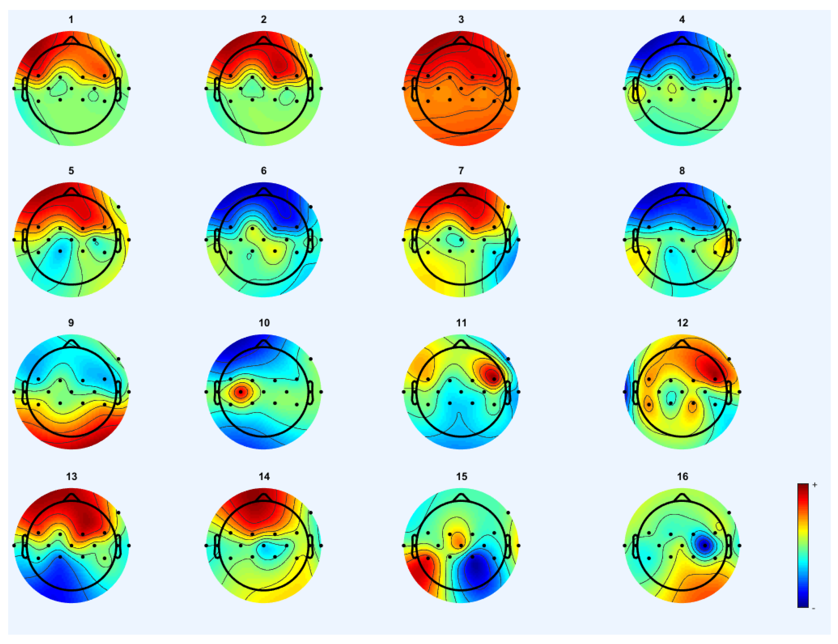
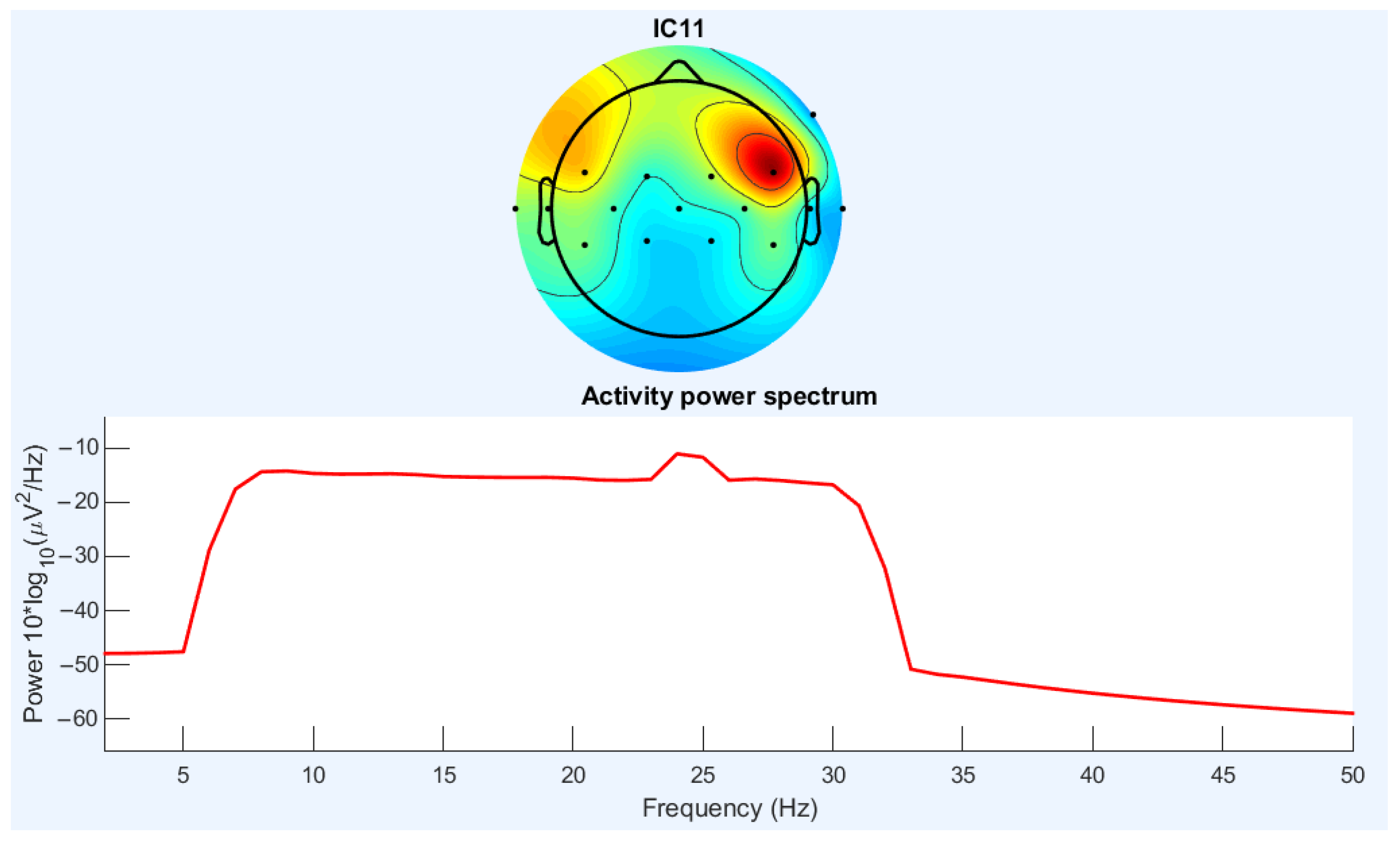
To demonstrate ICA-amplified neural signals, we created four samples of ICA topography. Many aids were identified from the sensory areas and formed a circular shape, which reflects our system’s emphasis on motor signals.
The ICA spatial filter attenuates the EEG signal in some parts of the scalp and amplifies the EEG signal in other parts of the scalp. To visualize typical signals amplified by the ICA spatial filter, ICA topographic diagrams were created for one person (person number one), and two mental images were created as graphs. To classify the two images, diagrams show which areas of the scalp have been weakened and which have been strengthened. A classification is made up of each chart because the weight and number of ICA components differ between classifications owing to different training data (Figure 18).
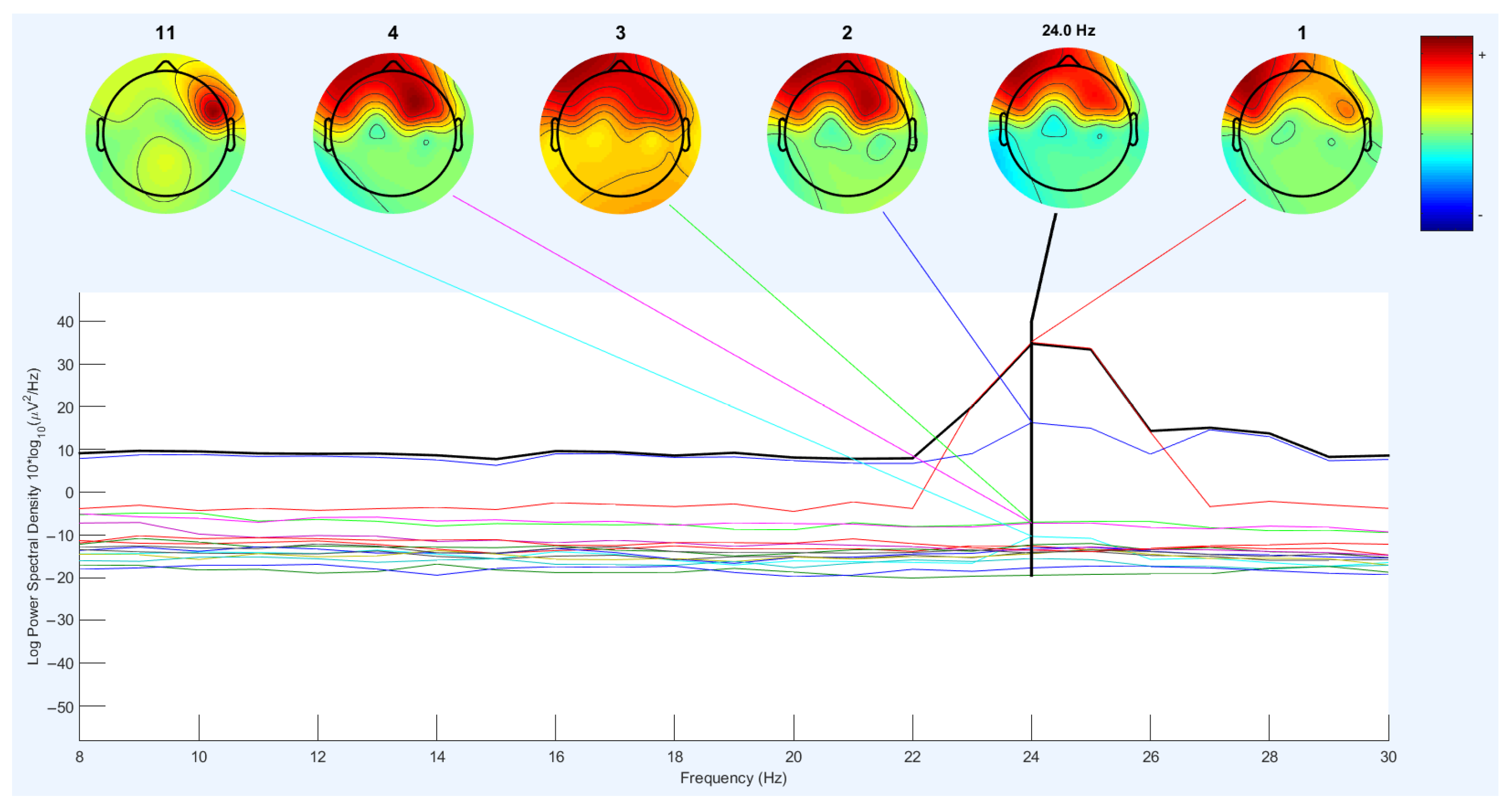
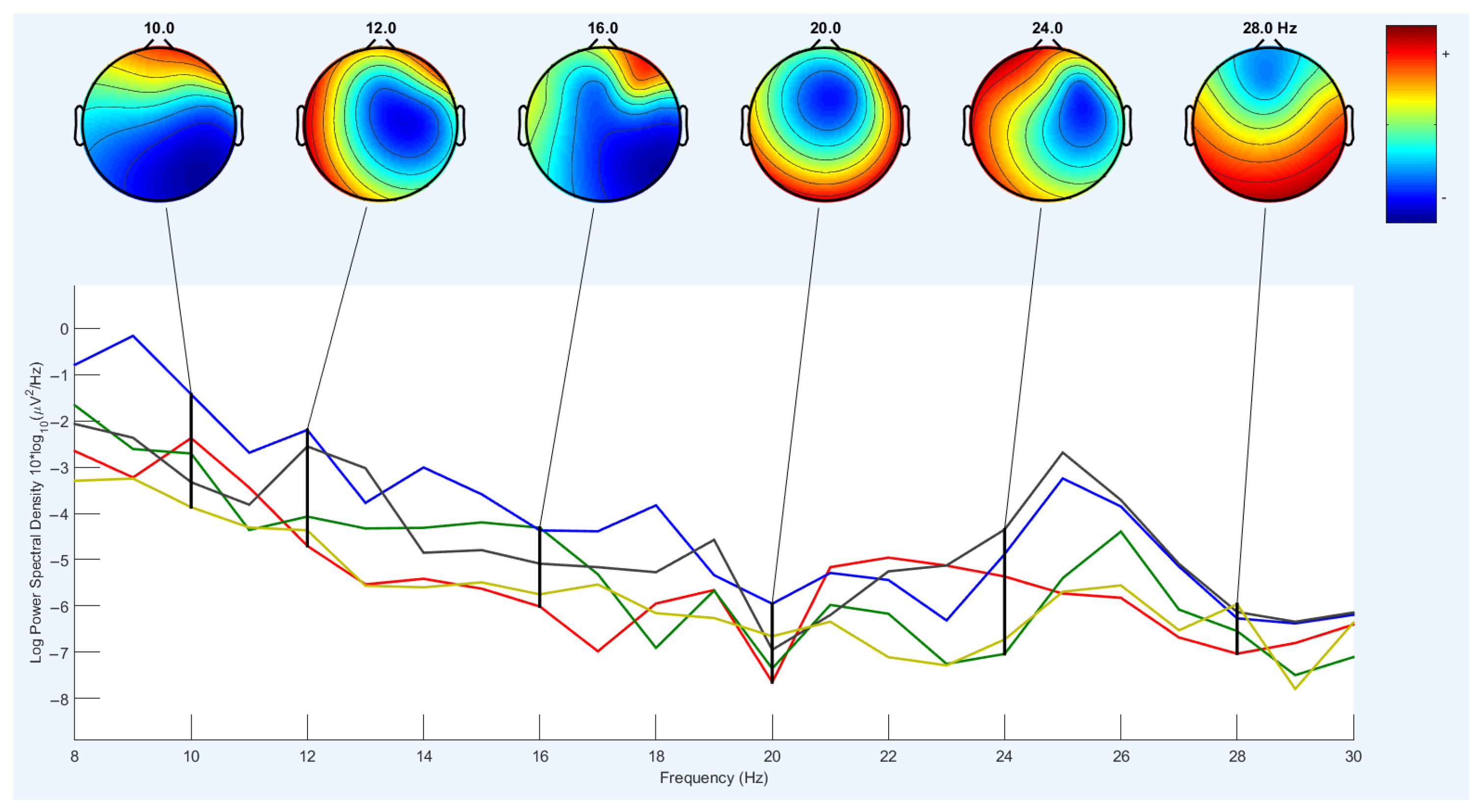
Figure 19 shows a frequency diagram with the power of the spectrum in the frequency range 8–30 Hz. It examines 16 channels for the two lip-reading concepts “A” and “M” in EEGLAB. The power spectrum was obtained between 10 and 20 Hz in the frequency range 8–22 Hz. Between the two intervals, it is slightly less and returns to the original state. These intervals are 14–14 Hz and 22–20 Hz. Then, between 24 and 22 Hz, the power of the spectrum increased to 40 Hz. First, between 25 Hz and 24 Hz, it decreases slightly at a slow rate. At approximately 25 Hz, it decreases with a steep slope and reaches 20. In the range of 28–26, it goes up and down slightly, and then the frequency returns to the power of the previous intervals, which indicates the power of the spectrum in this range, which increases during imaging.
Figure 19 shows a frequency diagram with the power of the spectrum in the frequency range 16–36 Hz. It examines 16 channels for the two lip-reading notions A and M in EEGLAB. The power of the frequency spectrum increases and decreases in the frequency range of 22–25, in which it increases up to 40 Hz; after the frequency range of 33 Hz, it returns to the lowest negative value. Between 16 Hz and 30 Hz, the power of the spectrum increases. This interval corresponds to the mental imagery interval. The different channels on the head show the energy at 25 Hz. This indicates that the power and energy of the brain are distinct when mentally imagining at a frequency of 25 Hz. Figure 20 and Figure 21 show the power output from Figure 19. However, the interval is between 8 Hz and 30 Hz.
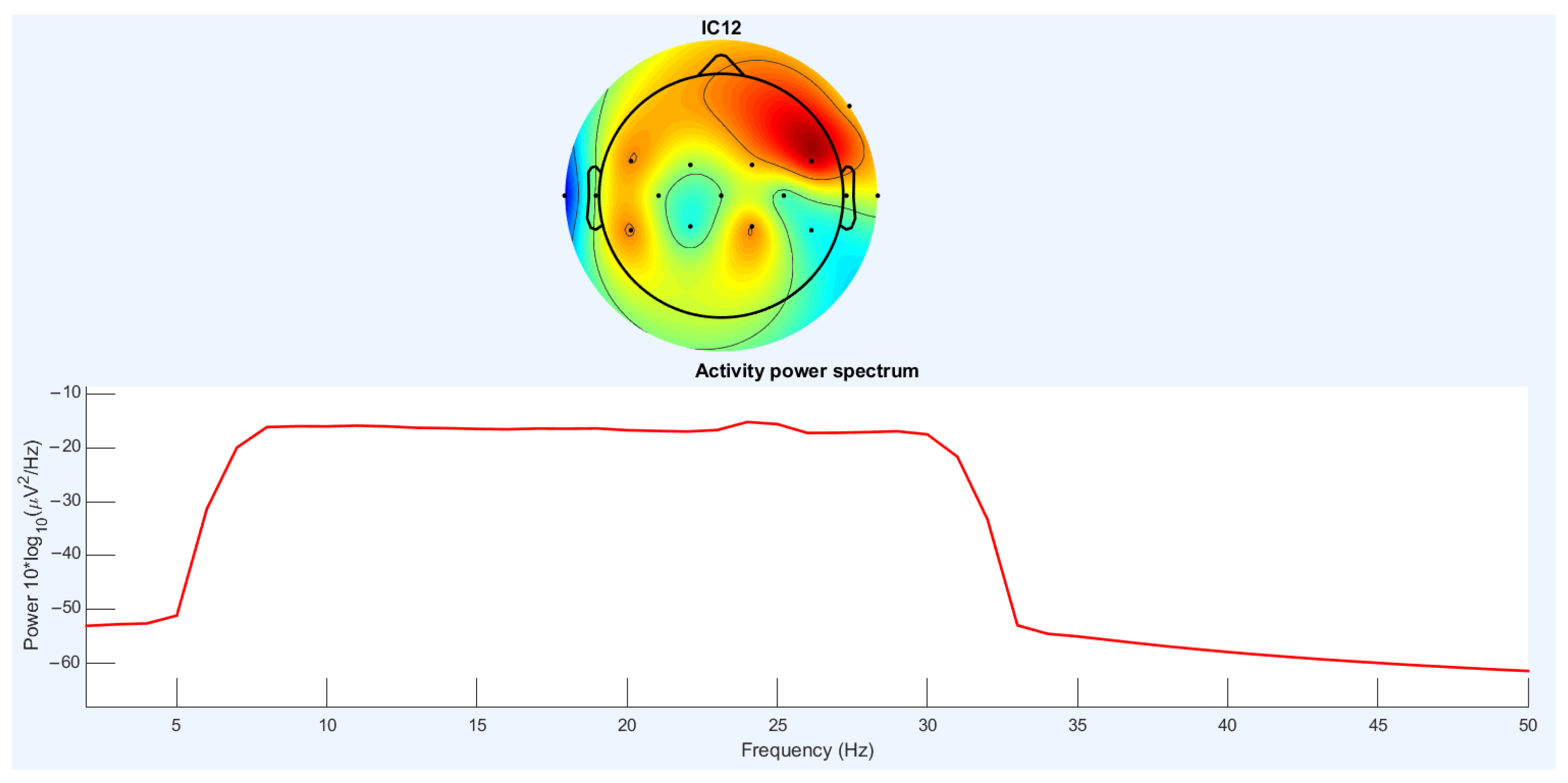
Figure 22 and Figure 23 show the frequency power diagram in the 0–50 Hz frequency range. The frequency power varied in the frequency range of 4–34 Hz. The frequency power increased between 4 and 8 Hz, and the frequency power decreased between 31 and 34 Hz. The frequency power was almost the same between 8 and 30, but in the range of 23 to 26, there was a slight increase and decrease in frequency. The amount of energy is also shown in different parts of the joint. Only one channel for the power of the spectrum is presented.
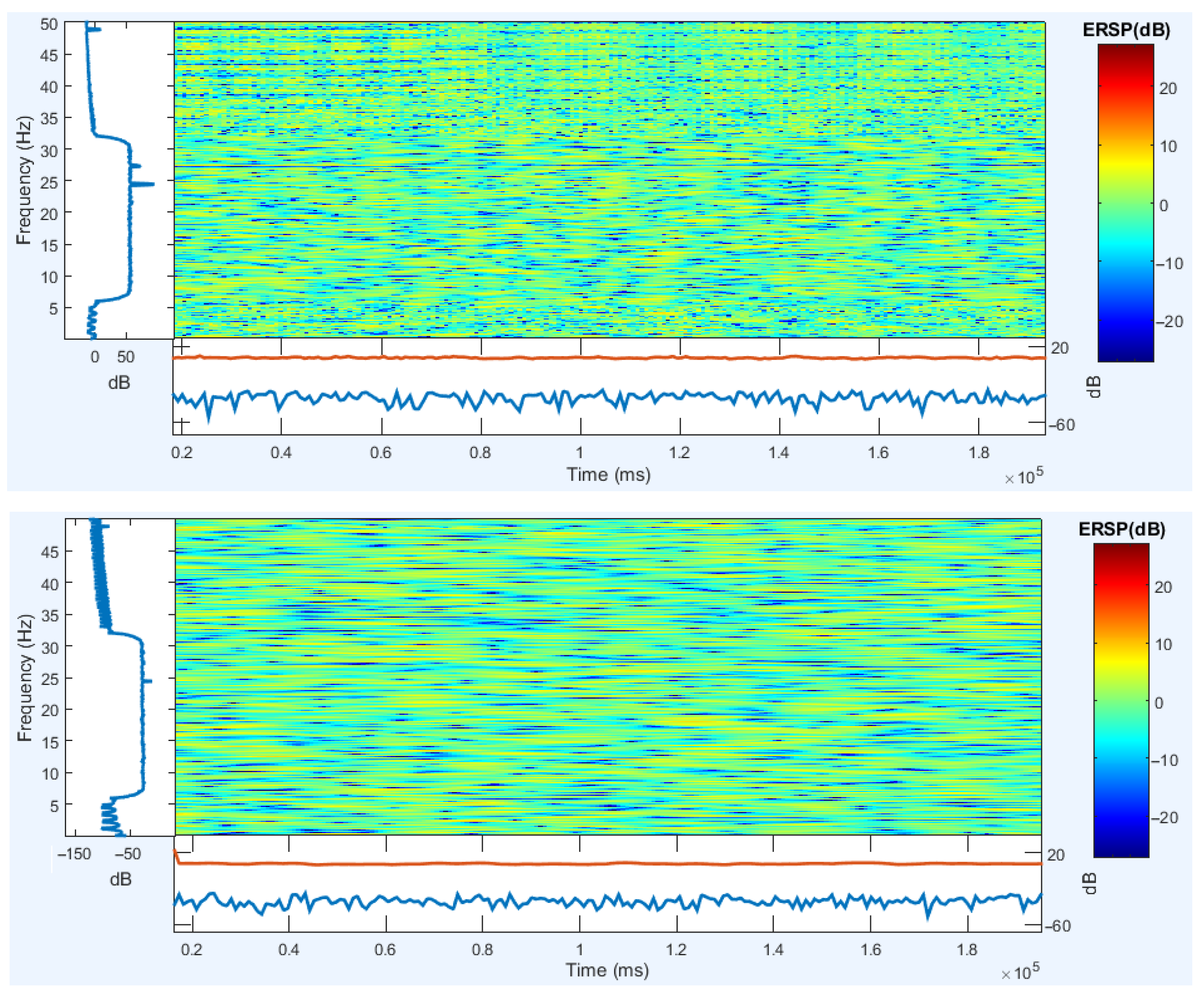
For comparison with previous work (speech imagery and mental tasks) [101], Channels C3 and C4 near Broca’s area and Wernicke’s area were selected to analyze event-related spectral perturbation (ERSP). Using complex Morlet wavelets, a single trial involved superimposing the energy spectrum by ERSP. EEGLAB was used to plot ERSP in this dissertation [100]. The ERSPs related to the two channels are presented for Subject 1 in the second and third steps in Figure 24.
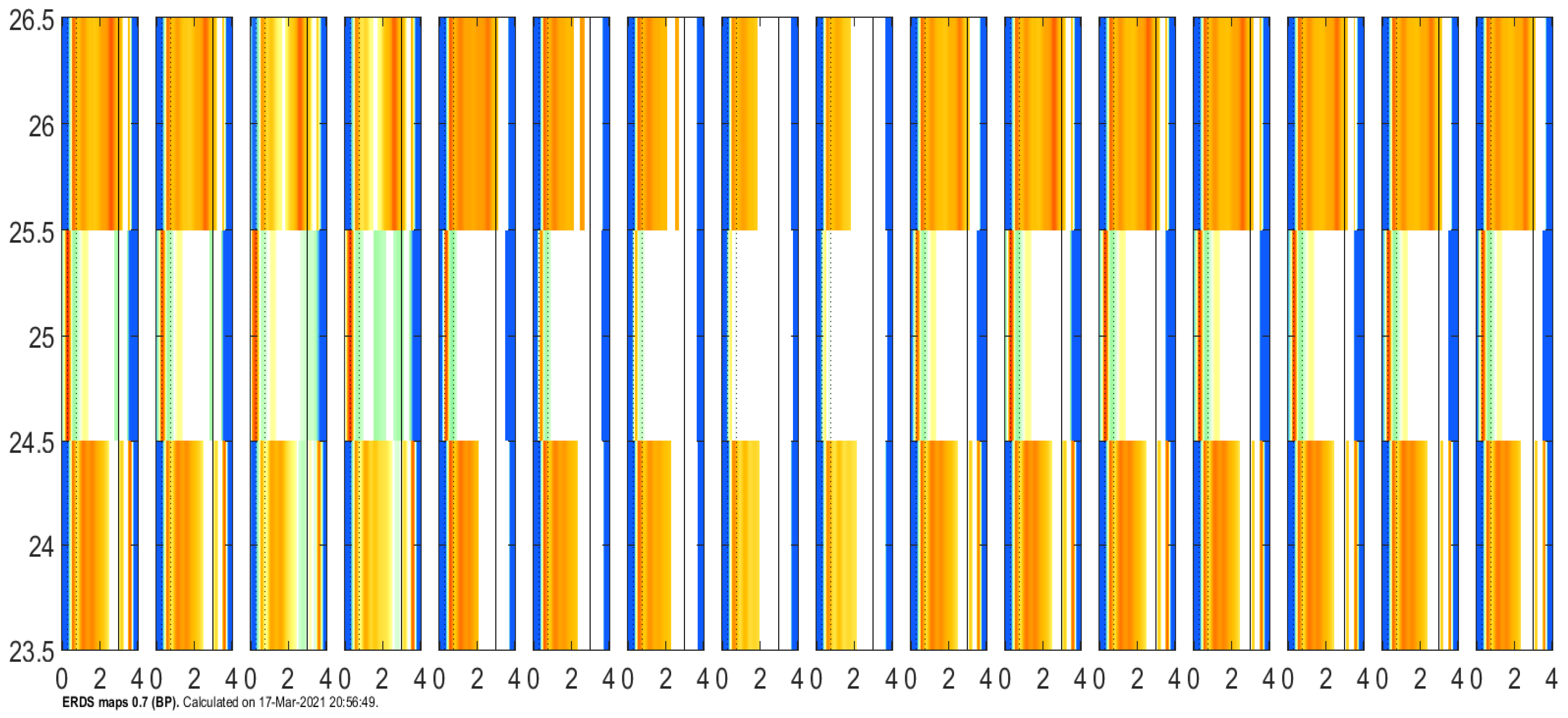
For comparison with previous work (speech imagery and mental tasks) [101], as in another article in the field of imagination, channel signals were referenced, and all 16 channels were selected for all areas of the brain, particularly the Broca and Wernicke regions. Using the complex Morlet wavelet, the experiment had an extraordinary energy spectrum by ERDS. CSP was used to draw the ERDS in this study. Figure 25 shows the ERDS in the frequency range of 23–27 Hz between 0 and 4 s. The imagination period for each activity was examined separately and simultaneously for two images, and different energy strengths were observed for all three expressed cases. Completely different frequency powers can be observed between the two notions, and various changes are observed between the two intervals between the distances of a frequency range. See Figure 25 for further details. Because of the noise in the signals, the rest of the frequency range was omitted.
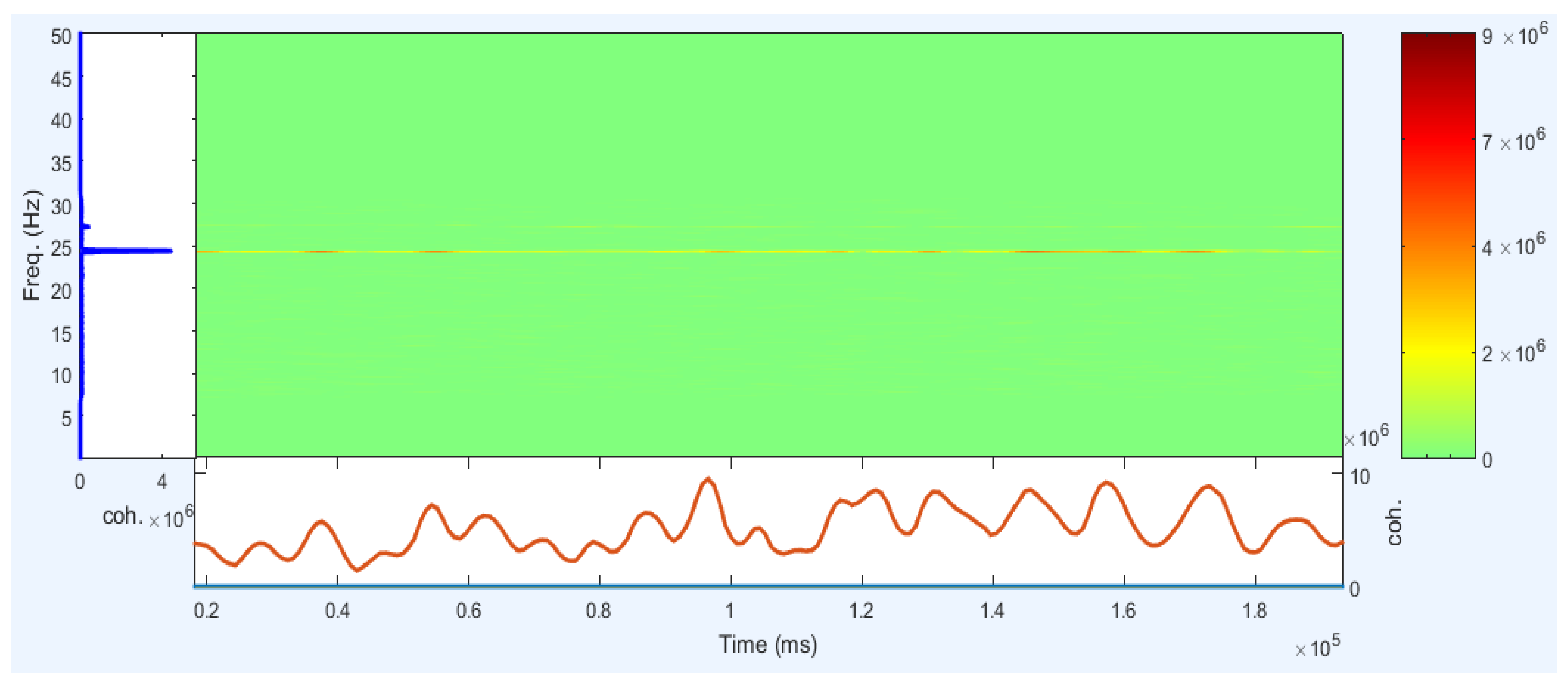
Cronbach’s alpha coefficient evaluates the temporal stability of ERD/ERS, as shown in Figure 26. The coefficients of the three time intervals were calculated during the experiment. The coefficients and specified yields are constant (>0.7), as shown in Figure 26.
To calculate the classification accuracy, the EEG signals of any subject were used in the training and testing sets using 5 × 10-fold cross-validation. The dataset was randomly divided into ten equal parts. Test spatial filters and classification were applied in each part of the test, and other parts were used to build CSP spatial filters. Subsequently, the feature values were extracted, and the classifier was trained. The average of ten different accuracies was used to calculate the overall accuracy. Five-fold cross-validation was also used. This training/testing procedure was repeated ten times with random detachment. The standard deviation was calculated for the analysis. The accuracy rates for the two subjects are listed in Table 1.
The best average validation accuracies of 3D lips for “A” and “M” in three subjects are between 66% and 70%, as shown in Table 1. Subject 1 with KNN had an accuracy of approximately 68.7% in the best state. The result for Subject 1 was approximately 54% to 68.7%, and that for Subject 2 was between 57% and 64%. Classification with KNN had a good accuracy of 62–69% relative to other classifiers. The SVM results are 61% to 68%, which are similar to those of KNN. It has a 1% accuracy, which is less than that of KNN. The accuracies of classification for Subject 3 are between those of the first two subjects. The signals of three subjects were sufficiently noisy. LDA had the lowest accuracy for the subjects, between 54% and 58%, which was weaker. The other classifiers performed well or less.

3.3. New Combinations of Signals Using Four Common Methods

3.3.1. CSP Using New Combinations of Signals

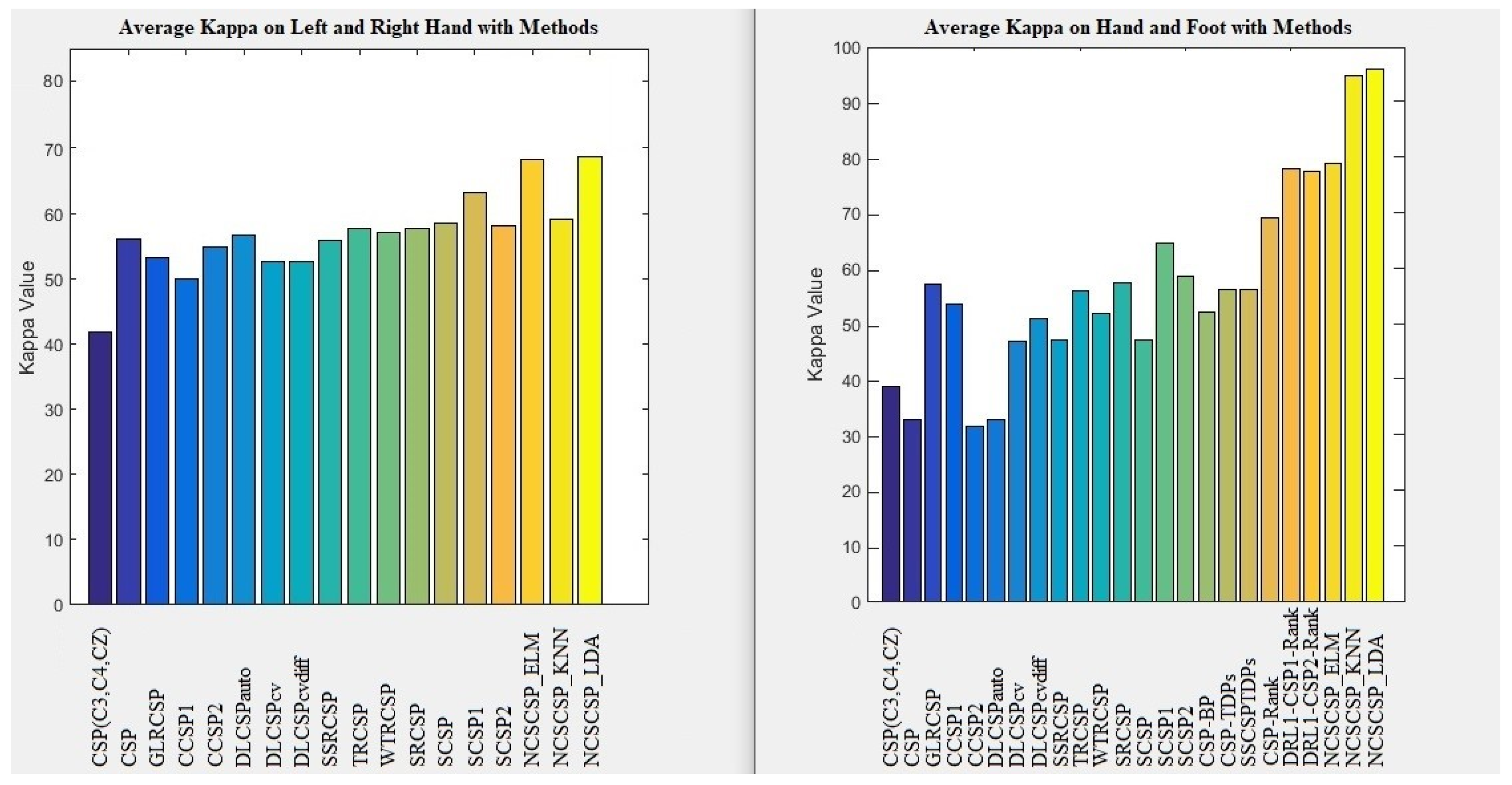
Table 2 shows the results of ten extracted features as five pairs of features by CSP. Three classifiers, LDA, KNN, and ELM, were used in our experiments. For the evaluation, we calculated the average kappa of all subjects for the left and right hands. Note that the new combinations of signals are presented as a combination of filter banks with their numbers. For example, a combination of filter bank I and filter bank J is expressed as “FB I and J”.
Based on Table 2, in the comparison of KNN and ELM, KNN has the lowest kappa. LDA has a slightly better kappa compared to ELM and KNN. The highest kappa value is for FB 5 and 6 (68.70%). CSP could remove noise well and extract good, suitable features for the left and right. LDA and ELM classifiers were successful in detecting suitable distinctive patterns between two classes, while there may be more of the same patterns for two classes.
In general, Table 3 shows the results of five pairs of features (ten features) for subjects with CSP that were used for our experiments with the LDA classifier. The details of subjects with LDA show slightly better accuracy (left and right hands). Except for two subjects, the rest have high kappa values (more than 60%), which indicates that some subjects achieved a low kappa value and other subjects achieved a high kappa value.
Table 4 shows the details of the average sensitivity of subjects for some of the new combinations of signals. It shows that the difference between left- and right-hand classes is less than 2%. And the difference between sensitivity and accuracy is small.
Table 5 shows the results of ten extracted features (five pairs of features) with CSP that were used for our experiments with three classifiers: LDA, KNN, and ELM. For the evaluation, the average kappa values of all subjects were calculated for the hand and foot.
Based on Table 5, in the comparison of KNN and ELM, ELM has the lowest kappa. LDA has a slightly better kappa than ELM and KNN. The highest kappa value is for FB 3 and 9 (95.90%). CSP can remove noise very well and extract excellent features for the hand and foot. The LDA and KNN classifiers are successful in detecting the most distinctive patterns between two classes.
In general, Table 6 shows the results of five pairs of features (ten features) for subjects with CSP that were used for our experiments with the LDA classifier. The details of subjects are shown for LDA, which has slightly better accuracy (hand and foot). All of the subjects have high kappa values (more than 90%).
Table 7 shows the details of the average sensitivity of subjects for some of the new combinations of signals. It reveals that the difference between left- and right-hand classes is less than 2%. And the difference between sensitivity and accuracy is small.
In Table 3 and Table 6, the p-values for our proposed method (new signals and CSP) with the LDA classifier based on CSP (C3, C4, CZ) [102] are calculated for the left and right hands and the hand and foot. In Table 2, for FB 5 and 6, the calculated p-value is 0.002 (p-values = 0.002), which is less than 0.05 and the others. In second place, FB 5 with 9 has a p-value of 0.003 (p-value < 0.05). In Table 6, for FB 3 with 9, the calculated p-value is 0.0061 (p-value = 0.0061), which is less than 0.05 and the others. In second place, FB 4 with 9 has a p-value of 0.0058 (p-value = 0.0058). The results show that the newest combinations of signals are statistically significant for the left and right hands and the hand and foot.

3.3.2. FBCSP Using New Combinations of Signals

In this subsection, the tables’ results are based on new combinations of signals. For comparison, two classifiers were used for all subjects. The minimum and maximum selected feature numbers are 5 and 40. Table 8 lists the average accuracies and kappa values for subjects with selected features and LDA and KNN classifiers. Table 9 lists the number of selected features checked for subjects with the LDA and KNN classifiers. In the following, the tables in this section are briefly described.
Table 8 is related to the selection of features from all features of new combinations of signals for the classification of the left and right hands. Table 8 shows the two best-performing classifiers, LDA and KNN. Using Table 8, 25 features were selected as the number of best features for LDA and KNN classifiers, which have kappa values of 68.13% and 73.15%. But the accuracy difference between the numbers of feature selections varies within 1%. This is the effectiveness of using many features that have little effect on the accuracy. The selection of the best features from all of the new combinations of signals could improve kappa by 5% in the second model compared to the first model in the best state.
Table 9 shows the best average kappa values for subjects with KNN classifiers for the right and left hands. The highest kappa with the selection of 25 features is 73.15% for KNN. The maximum and minimum kappa values are for Subjects 8 and 3 and Subjects 2 and 4, with the largest difference. The p-values for all of the cases are between 0.0039 and 0.0042. This means that they are significant (p-value < 0.05).

3.3.3. Lagrangian Polynomial Equation Using New Combinations of Signals

In this subsection, the results are explained for normal sub-band signals and new combinations of signals for single electrodes. The results in Table 10 show the average accuracies of new combinations of signals for Channel 5 using ELM and LDA. Table 11 shows 1 and 30 selected features for a channel using nine filter banks.
Table 10 shows the results after converting data to coefficients by using the Lagrangian method for Channel 5. The 30 features selected as the best coefficients were considered for classification. The results increase from 51% to 58% for some combinations of filter banks. In comparing the best new combination of signals relative to the rest, the results vary between 2% and 6%.
Table 11 shows the accuracy results when using 1 best feature and 30 best features of formula coefficients with three classifiers (left and right hands). For the ELM classifier on Channel 1, selecting the 30 best features compared with selecting 1 best feature results in a 3 to 5% increase in accuracy for different filter banks. But for Channel 2, this change is between 3 and 8%.
These coefficients are coefficients of the Lagrangian polynomial equation with different orders, which are achieved based on the effect of the pattern in signals. The main purpose is to find the best and most effective coefficients. Figure 27 shows the results of ELM and LDA classifiers with three channels for 1 to 30 selected coefficients. Using one coefficient has a higher accuracy relative to other numbers. When selecting more coefficients for classification, the accuracy decreases. This means that it is more effective to use the coefficient of one feature, and then the effectiveness of coefficients decreases. These results are for non-important channels. Channels in the center of the brain (Channels C3, C4, and CZ) have increased importance because the locations of these three channels are in front of the brain.

3.3.4. PCA Using New Combination of Signals

In this subsection, the results of PCA are summarized in Table 12 and Table 13. For illustration, Channels 8 and 12 with the ELM classifier on the left and right brain hemispheres are selected. Normal sub-band signals and new signals (FB I with J) are used for investigation. The results with more information are described below.
Table 12 and Table 13 show the results of PCA, in which computational operations (sorting) were performed to reduce the features. But no features were reduced for classification. Table 12 reports the results of Channels 8 and 12 on the left and right hemispheres of the brain with the ELM classifier with normal signals (filter banks).
Finally, the average accuracy for Channels 8 and 12 increased by 17% and 18%, respectively, when comparing new combinations of signals to normal filter banks. For Channels 8 and 12, FB 1 and 5 achieved the highest average accuracy for the subjects.

3.3.5. Discussion of Results

Our proposed methods were compared with different previous methods based on CSP. For these comparisons, two datasets with new signals using CSP and FBCSP were used. Therefore, this paper generally explains the effectiveness of our proposed methods compared with previous methods.
Table 14 uses different methods to compare the kappa of our proposed method (new signals and CSP) with those of CSP, GLRCSP, CCSP1, CCSP2, DLCSPauto, etc. [103]. The highest average kappa was obtained by our proposed method using a new combination of signals with CSP (FB 5 with 6 (68.60%)), which is higher than those of the other mentioned methods, with the smallest difference obtained by SCSP1 [103] (5%) and the largest one obtained by CCSP1 [103] (18%). It has an acceptable kappa (68%), which is sufficiently (8%) higher than the standard kappa (60%). With the proposed method (new combination of signals with CSP), the majority of the subjects obtained good kappa values (above 60%). But Subjects 2 and 5 had the lowest kappa values (between 45% and 50%). These kappa values are listed in Table 14 for the right and left hands. The p-values for all of the methods were calculated: most of the methods have p-values of less than 0.05 (p-value < 0.05), and some methods have values of more than 0.05 (p-value > 0.05). For new signals with CSP using LDA and ELM, the p-values are less than 0.05 (p-value = 0.009, p-value = 0.004, p-value < 0.05), and for new signals with CSP using KNN, the p-value is 0.052, which is higher than 0.05 (p-value = 0.052, p-value > 0.05).
Table 15 compares the kappa values of different methods [103,104] with that of the proposed method (new signals and CSP). With the highest value of kappa, 95.89%, the proposed method greatly outperforms the other methods. Kappa values for the new signals with CSP using LDA for individuals are between 94% and 97%, which is a very high value for kappa. It is demonstrated that our model has increased accuracy and kappa to the highest values. For new signals with CSP using three classifiers, the p-values are less than 0.05 (p-value = 0.034, p-value = 0.010, p-value = 0.010). The three lowest p-values belong to SSCSPTDPs, NCSCSP_KNN, and NCSCSP_LDA, with p-values of 0.005, 0.010, and 0.012, respectively.
The left side of Figure 28 shows the average kappa from Table 16 for different methods implemented for the left and right hands. The right side of Figure 28 shows the average kappa from Table 17 for different methods implemented for the hand and foot. The bar chart shows that the highest bars are for our proposed method relative to other methods.
Table 16 compares the best accuracies of results obtained for the hand and foot with different methods [105] of CSP with/without filter banks with our proposed method (new signals with CSP). The results obtained with LDA with the highest accuracy value (97.94%) compared to the previous methods mentioned in Table 15 show an advantage of between 5% and 9%. In total, the highest accuracy value (98.94%) is very good for this database with five subjects. For Subject 4, LDA with the new signal obtains the highest accuracy value (98.92%) with statistical significance (p-value = 0.0107, p-value < 0.05). In comparing the new signal with CSP using LDA to common spatial pattern (CSP), common spatial-spectral pattern (CSSP), and CSSSP (common sparse spectral-spatial pattern), the accuracy is improved by 6%. All of the methods are statistically significant (p-value < 0.005). The results of our method are similar to those of other methods, with small differences.
Table 17 shows the comparison of the best kappa results obtained for the left and right hands with different CSP methods [105], which are considered for all or some channels. Subject 1 achieved the best kappa value with CSP and 8.55 and 13.22 channels. Subject 2 with our proposed method and ELM and Subject 3 with our proposed method and LDA achieved the best kappa values. The best average kappa was obtained by the new combination of signals with LDA (68.6%). In an overview of subjects, it is deduced that Subjects 2 and 5 have the lowest kappa values, and Subjects 3 and 8 have the highest kappa values.

3.4. New Linear and Nonlinear Bond Graph Classifiers

Table 18 shows results related to the performance of the proposed linear classifier, SVM, and LDA. These results are based on the preprocessed public speech imagery dataset that was examined. The results revealed average accuracies of 53.45%, 53.84%, and 61.02% for Channels 1, 2, and 4, respectively, with the second proposed model and 65.19% for Channel 3 with LDA. The result for the first proposed model is 60.44%, which is 5% lower than that of LDA and 5% higher than that of SVM. The first proposed model and LDA both obtained good results of approximately 84.21% from Channel 3, and the highest result obtained was 86.84% accuracy for the third subject and Channel 4 using two new models. In general, with this preprocessed dataset, the new models achieved suitable performance and accuracy. The remaining results are presented in Table 18 for further review.
Table 19 shows the performance results of the proposed nonlinear classifiers SVM, LDA, and KNN. These results are similar to those in the previous table for the preprocessed speech imagery data examined. The results show average accuracies of 57.94%, 59.49%, 65.71%, and 62.29% for KNN, which had the highest values. The accuracy of the proposed algorithm was 5–6% lower. Our results were checked for each individual. The proposed model exhibited a good performance in some channels. The first subject performed 5% better in Channels 1 and 3. The third subject with Channel 1 was 10% better than those of LDA and KNN. However, in many cases, the others exhibited the best performance. Table 19 presents the results of the nonlinear performance comparison and interpretation.
Table 20 and Table 21 show the proposed linear and nonlinear classifier performance, respectively. These results are related to the preprocessed left- and right-image notion data examined. Table 20 lists the 22 channels with the total number of individuals. Nine of the brain channels had between 50.69% and 54.47% accuracy, which are related to the better performance of the proposed linear model. Eleven channels have between 50% and 53.85% accuracy, which is obtained with SVM, and four channels have between 50.38% and 53.47% accuracy with LDA, which has the best average. The two channels have the same degree of accuracy, as is intended for both.
The best results for each subject are related to the highlighted categories listed in Table 21. For the best performance accuracy, Subject 5 had 60.14% accuracy for Channel 22 with the SVM classifier, and Subject 7 obtained the best accuracy of 61.80% for Channels 6, 5, and 7 and 61.11% accuracy for Channel 13 with the LDA classifier. Finally, the proposed method for Subjects 4, 5, and 9 with Channels 15, 12, and 13, with accuracies of 60.41%, 61.11%, and 60.41%, respectively, showed good performance. As shown in Table 21, only one channel with an average accuracy of 49.76% belonged to the proposed method. The rest of the accuracies were distributed between different models, which achieved good accuracy. Further details are provided in Table 20 and Table 21.
In Table 22 and Table 23, the test data results on the two benchmarks are shown as linear and nonlinear, respectively, and were obtained using the proposed method. In the linear model, the best results were obtained by SVM. LDA and the proposed method have the lowest results on the benchmark sonar, with 3% and 4% differences, respectively. The proposed method, with 82.59% accuracy, was only 0.5% lower than LDA, with 83.04% accuracy. Essen indicates the proximity of this method to the LDA method. In Benchmark Wisconsin, the differences were slightly higher. The proposed method, with 67.39%, has a difference of 7% from SVM and 2% from LDA. The performance of the nonlinear classifier is also seen in Table 22 and Table 23, with a difference of 6% to 15% compared to other classifiers. This method can be used as a supplement to SVM, which has a good performance when the noise level is too high or too low.

3.5. Deep Formula Recognition Results with Root Interval Recognition Classifier

The results of the root intervals of the formulas based on the size of the conversion and selection window on Channel 8 for ten people are shown in Figure 29 and Table 24. The first six subjects are shown in a bar graph model, and the last three subjects are shown numerically in Figure 29 and Table 24. The average accuracy results were between 48 and 52 percent for the different band filters. Each filter bank was analyzed separately. For a better understanding, some variables are stated (M1 stands for formula window size 7, M2 stands for window size 14, and M3 stands for window size 35; S represents the selected window size for blending).
The results in Figure 30 and Table 25 are expressed in the same way as the results in Figure 29 and Table 24. The difference is that the results are for Channel 10, which investigates nine subjects. Channel 10 resembles Channel 8 used for some filter banks, which obtains a maximum average of 52%. In this channel, the best accuracy was for Subject number 7 at 59.03% and 59.07% for bands 4 and 6, respectively.
The results in Figure 31 and Table 26 are similar to those in the previous figures and tables, and the only difference is in the channels, with Channel 12 being investigated in this test. The best results for Subjects 3, 5, and 7 are that Subject 3 had the best performance with filter bands 4 and 1 at 58.79% and 57.23%, and Subjects 7 and 5 had results that were1% to 2% lower than those of Subject 3, respectively.
We can draw conclusions based on the results shown in Figure 30 and Figure 31. The highest accuracy was related to Channel 8, followed by Channel 10, and the weakest channel was Channel 12. The difference in accuracy between the channels ranged from 1% to 2%.
Table 27 presents the results of the best accuracy for a subject with a K-fold of 10-10. The results show that they have the usual accuracy with high noise. When there is more noise, it is difficult to detect the roots, which leads to a decrease in the accuracy. This is true for all classes. If we examine one of the implementation steps individually, some show the formula closest to the differentiation formula between the classes. For example, using the near-differentiation formula as the differentiation formula can yield the best result. In other words, the best accuracy is 82.8% for Fold 9 in Step 8, indicating that the differentiation roots are close to the original (ideal) differentiation roots. In other words, Fold 9 can be used to discover formula roots for similar training experiments and achieve high accuracy. Owing to high noise, the formula roots in Fold 2 are not obvious roots for classification.
Table 28 presents the results of the last method, which showed weaker results. The formula coefficients were classified as features by the classifiers. The highest accuracy was related to the random forest (RF).

4. Discussion of Results

4.1. General Discussion about Speech Imagery with Mental Tasks

Based on the method used by deaf people, this study introduces 3D and 2D lip methods for speech imagery as a potential communication approach in the future. The 3D lip is considered an easy method for general communication. Another method can be used to enable communication in different areas.
In another study, audio–visual images used only five sounds, but it was impossible to create another sound. Another article reported the use of a mental task with speech imagery, but it was difficult for the subject to imagine for a long time. It is difficult to visualize the writing of strokes and rotation with audio characters. This idea is only applicable to Chinese characters. Our proposed model uses two models that are combined for the basic sound of languages. It is easier to use mental tasks instead of imagination.
Each model uses two tasks with different complexities for mental work. In contrast to 2D, 3D can support all of the characters. This indicates that 3D imagery is better than 2D imagery given the same model. However, further research is required to improve its accuracy. Additionally, 3D lip imagery can be used to learn in everyday life. It is easy to imagine this for all age groups. Questionnaires also show that most people can easily become distracted when performing mental tasks.
Before the study, the activities of the sensorimotor cortex, Broca’s region, and Wernicke’s region were particularly significant [25,26]. Our research used an identical model to other mental research to focus on the primary and pre-movement cortexes, temporal cortex, and complementary motor area (SMA). Our study was driven by a second motivation, which is to offer this method to patients with spinal cord injuries. In addition, this type of amputation, unlike physical amputation, makes it possible to retain motion pictures for a long time.
According to ERSPs, the effect of the EEG energy signal is determined only in a de-terminated frequency range. Therefore, the frequency range was verified before the ERS maps were drawn. Each topic had a different frequency range. The stability calculation based on the EEG band was not considered (e.g., theta, alpha, and beta groups). Our study offers a specific range for most channels.
The stability of the ERD/ERS values was tested using Cronbach’s alpha coefficients. They achieved the highest compatibility [26] for word outcomes in subjective subtraction and spatial navigation tasks. As with Friedrich’s results, task “A” showed a higher stability in both phases. Therefore, based on the specific activity, the temporal stability of ERD/ERS also varied in three time intervals. The ERD and ERS coefficients were the most stable. This depends on the attention paid to the subject at the beginning of the imagination.
It Is difficult to distinguish between EEG signals in the same channel using two different tasks. However, in each dimension, imagination in a channel is different for two activities. However, using ERD/ERS diagrams of the two works in the same figure can indicate the difference. This difference is shown by increasing the EEG energy amplitude. The range of “A” is more like “M” and like any other task (characters).
By testing several brain regions of the left frontal lobe and the posterior temporal lobes, the semantic processing relationship is revealed by the semantic execution system of extracting semantic information. Unlike stroke writing, lip and language synchronization are also learned for short-term learning and may be processed by a wide range of cortical areas. The motor cortex region has low task efficiency. Despite slight changes in body movement, EEG signals from lip synchronization are appropriate. This is similar to a BCI based on motion pictures that include imagined movements of the right hand, left hand, tongue, and foot. The upper parietal lobule was associated with image rotation. It is possible to clearly distinguish EEG signals from different areas.
There is a clear difference between the results for these two issues. It is based on the different educational backgrounds of individuals and their understanding of the experimental tasks. Therefore, instructors perform different mental tasks. The differentiating characteristic is that the power spectra of the EEG signals in the cortical wall are significantly different. These models are able to complete all of the original sounds. Each language can then use a base model for communication. These are easy to model. With the proposed method, imagination can last for a long time without further fatigue, and the appropriate model can be selected for a certain region and language.
Previous studies [106,107] have investigated cortical activity and number classification performance during tactile imaging (TI) of a vibrating stimulus in the index, middle, and thumb fingers of the left hand in healthy subjects. In addition, the cortical activity and classification performance of the TI combination with the same mixed motor imagery (MI) were compared with the same TI figures in the same subjects. The results of this study demonstrate that tactile composite images can be a suitable alternative to MI for BCI classification. This study contributes to the growing evidence supporting the use of TI in BCI applications, and future research can build on this work to explore the potential of a TI-based BCI for motor rehabilitation and the control of external devices. Our goal is communication based on lip reading, which is a general task for communication. This method was first studied using an MI. In addition, the TI method can be used for verification. This method can be easily implemented and used in practical applications. However, further research in this field is required. Some of the new methods presented can lead to the quick realization of this method for future communication.

4.2. General Discussion about Combinations of Filter Banks

The best results for the new signals with CSP and three classifiers are compared with different previous CSP and FBCSP methods. The advantages of these new contributions are presented for comparison. Emphasis is placed on solving the problems mentioned in the introduction by identifying the highly distinctive features of brain activities for improved classification. It is clear from the results that the proposed methods obtain better values than previous methods. Therefore, this subsection compares the effectiveness of our proposed method with previous methods. Finally, in the next subsection, we discuss our contributions and results. This explains the problems and provides the main solution for solving these problems.
Based on [22,23], important distinctive patterns of brain activation, such as the left hand and right hand, are in the 4 Hz to 40 Hz frequency domain. Extracting features from the large-scale frequency domain produces the most similar and distinctive patterns, which leads to the extraction of ineffective features. Considering suitable frequency domains helps researchers extract effective features by separating similar patterns from most of the distinctive patterns. Based on [20,23], it is necessary to find small and suitable frequency bands with important distinctive patterns for high-accuracy classification. Based on most research [15,16,17,18,19,20,21,22,23], the most distinctive patterns are distributed in different frequency domains as small, fixed filter banks. The distribution of distinctive patterns in the 4–40 Hz frequency domain led us to consider the combination of two limited filter banks (frequency domains) to discover the most important distinctive patterns of brain activity signals. New combinations of signals can express low- and high-accuracy classifications by measuring distinctive patterns with a combination of different frequency bands, which express the support rate of the most distinctive patterns as a distinctive formula.
Unlike most previous papers [15,16,17,18,19,20,21,22,23], this study focuses on the combination of filter banks (limited frequency bands) using general CSP methods and a Lagrangian polynomial equation for extracting coefficients (features). The purpose of combining the two filter banks is to solve the previous problems. These problems are as follows. (1) In large frequency ranges, it is not possible to distinguish the most accurate location of the most distinctive patterns. In other words, the frequencies cover distinctive patterns of brain activity (left and right). The most distinctive patterns can be lost when creating smaller frequency bands. (2) The amount of noise is very high in high-frequency bands. (3) Reducing the quality of narrow filter banks leads to more degradation of raw EEG signals. This is the general composition model (various models) that has been described. In this study, as a small part of our ordinary model, two filter banks were implemented as new combined signals to eliminate these problems to some extent. In our study, the kappa of FB 5 and 6 with CSP for the left and right hands was improved by 5%, the kappa of FB 3 and 9 with CSP for the hand and foot was improved by 10%, and the accuracy of FB 5 and 6 with PCA was improved by 18% for a single channel. Therefore, for the two brain activities, the hand and foot achieved high accuracy and kappa, which include 4 Hz to 8 Hz (theta) with 8 Hz to 12 Hz (alpha). And 16–36 Hz (beta) had more noise, and the distinctive patterns were not high in other combinations similar to these combinations. In addition, statistical significance was calculated and was a suitable value.
The purpose of the new combinations of signals is to increase the classification accuracy and discover the effectiveness of the two combination sub-bands, which leads to a new signal reaching the near-optimal signal. However, it does not reach the global optimal signal. Therefore, a distinctive pattern differentiating the two activities was identified in these sub-bands. There are two states. First, some frequency bands can include the important parts of the main formula, which is the main formula pattern for distinguishing between activities, and other frequency bands that are less effective or less important in the main formula for distinguishing between activities. Second, these sub-bands contain the main differences and similar parts between the formulas for the two activities.
The detection of brain activity also depends on the formula of the classifiers. Therefore, this has an acceptable influence on the detection. In our study, the LDA and KNN classifiers showed good performance with the ELM classifier. The three classifiers show similar performance in that some new combinations of signals have high accuracy compared with other new combinations of signals. Therefore, selecting a convenient classifier is important for classification.
In this study, the Lagrangian polynomial equation is introduced to extract coefficients as features, which leads to the selection of the best coefficients of the formula for increasing performance. An effective distinctive pattern was applied to one or more coefficients. In our experiment, a limited time of approximately 1 s was tested for effective brain function (three channels in front of the brain) as one feature. Owing to the conversion of 0.5 and 1 s of data to formulas, it is impossible to describe the main relationships of coefficients with brain activities. It is necessary to examine different brain locations, large-scale frequency domains (8–30 Hz), and different recording times for EEG signals to find the relationship between the coefficients and the order and the relationship between the brain location and the duration of brain activity.

4.3. General Discussion about Bond Graph Classifier for Supplementation of SVM in Noisy Signals

This study introduces a new supplement to the SVM classifier for noisy data. This idea is similar to a hyper plane model, which is different from the linear SVM model for finding a hyper plane. When the data are very noisy, the classifier does not need to be highly sensitive in finding a very good boundary. Our classifier was not very sensitive in finding suitable borders in noisy data. This can increase the performance to between 2% and 3% accuracy.

4.4. General Discussion about Deep Formula Detection and Root-Extracting Classifier

Compared with QRNN, the proposed method is 3% less accurate. Our best results (63.15%) were 3% less accurate than those of QRNN (66.59%) under the same test conditions. In comparison, RAW (64.27) had a 1% lower accuracy. FBCNN with the same weight can achieve this accuracy or less.
When compared with CNN models, our proposed method has a 10% lower accuracy than CNN, 7% lower than CNN, 17% lower than DBN, 19% lower than RNN-GRU, and 16% lower than RN-LSTM.
In the two-class classification, our proposed method achieved 12% lower accuracy than CNN (Relu, tanh(FC), and sigmoid(FC)), 17% lower than CNN, and 10% lower than CNN (ERlu (conv), and softmax (FC)).
The essential purpose of deep neural networks is to extract complex features to distinguish patterns and increase the accuracy. Therefore, classifiers can obtain the best accuracy and discrimination using these complex features.
This paper presents, for the first time, a new and different method called deep recognition instead of deep learning, which requires identifying the roots of formulas for classes. This study introduces a new model for artificial intelligence and machine learning. By developing this model, a model for recognizing the roots of formulas for activities can be presented as deep detection, which can help expand and further understand artificial intelligence fields. Based on this formula, the reasons for the influence of the environment formulas on that formula can be examined. However, in deep learning, one cannot go into detail because the layers do not express the information in detail. Due to the high complexity, it is not easy to interpret the layers.
The deep formula detection structure is such that the first layer, all electrodes, or channel data are converted into a formula model. In this study, only one channel was used, but with development, two or more dimensions can be used, but the implementation is somewhat difficult. After the first layer, processing was performed on the formula model. Therefore, this study changed the processing model from a data-processing structure to a formula-processing structure (the first layer converts the data into a formula). In the other layers, the formulas are converted into a simple formula. After the extraction in the last layer, formulas are sent to the classifier to extract and identify the roots. Our proposed model requires further research to be excellent, although this model can obtain 55–60% accuracy for a single channel. However, this method is less accurate. In articles using similar data (except for the formula model), there is less difference between them in a single channel. The maximum accuracy for a single channel is between 60 and 70. One of the reasons that it is lower than the others is that it uses a frequency range of 4 Hz for processing. The rest use a 26 Hz frequency for processing. The acceptable amount for one channel is compared to articles with results in various contexts in this field (limited frequency range, single channel, appropriate window size, appropriate function definition, etc.). By solving this problem, the accuracy can be increased to between 60 and 70 or higher, because most information is lost during the creation of the filter bank. Other reasons can be related to the following: (1) choosing a window of the right size to convert the data into a formula; (2) choosing an appropriate sample size for the coefficients; (3) selecting or creating a suitable sampling function for the coefficients; (4) choosing the appropriate frequency range; (5) choosing the appropriate interval in which the root is located; (6) selecting long times in the first run of one second.
Finally, by developing the proposed method, it was possible to discover the main formula for complex activity. The novelty is that we convert the specified roots for each class that is different from other classes into a formula. We also convert the formula of the common roots of all classes into a formula. By combining the common formula with the formula of each class, the general formula of that class is obtained. In fact, we should first seek to know a simpler activity formula. Then, we can precede to the discovery of complex activity formulas. This can be one of the correct ways to solve complex problems. This can explain the hidden part of the system that prevents its further understanding. Different formulas can be introduced for the analysis to determine the best methods.

5. Conclusions

Most researchers have focused on developing new methods for the future or improving basic implemented models to identify the optimal standalone feature set. Our research focused on four ideas. The first introduces a future communication model, while the others are improvements of old models or methods. (1) A new communication imagery model instead of a speech imager using a mental task: speech imagery is very difficult, and it is impossible to imagine the sounds of all characters in all languages. Our research introduces a new mental task model for all languages called lip-sync imagery. This model can be used for all characters in any language. This study was the first to use lip syncing for two sounds or letters. (2) New combinations of signals: Selecting an unsuitable frequency domain can result in inefficient feature extraction. Therefore, domain selection is important for processing. The combination of limited frequency ranges provides a preliminary method for creating a fragmented continuous frequency. For the first model, two intervals of 4 Hz were examined as filter banks and tested. The primary purpose was to identify the combination of filter banks with 4 Hz (scale of each filter bank) from the 4 Hz to 40 Hz frequency domain as new combinations of signals (8 Hz) to obtain good and efficient features by increasing distinctive patterns and decreasing similar patterns of brain activities. (3) A new bond graph classifier to supplement the SVM classifier: When linear SVM is used with very noisy data, the performance is decreased. However, we introduce a new linear bond graph classifier to supplement the linear SVM for noisy data. (4) A deep formula detection model: The data in the first layer are directly converted into formula coefficients (formula extraction model with Lagrange formula). The main goal is to reduce the noise in the subsequent layers for the coefficients of the formulas. From the second layer to the last layer, by using different functions, the effective formula coefficients (differentiation formulas between classes) are extracted so that the coefficients that have the most similarities between classes are removed in different layers. The effective coefficients of the formula are sent to the classifier of the new model to extract the roots of the members and identify the common roots of the class. The results range between 55% and 98%. The lowest result is 55% for the deep detection formula, and the highest result is 98% for the new combination of signals.

Author Contributions

A.N. conceived of the ideas. Z.F. helped to complete the ideas. A.N. performed the numerical simulations. Z.F. validated the results. A.N. wrote the original draft. Z.F. and A.N. edited the manuscript. All authors have read and agreed to the published version of the manuscript.

Funding

This research was funded by the National Natural Science Foundation of China, grant number 61876147.

Data Availability Statement

Datasets are public datasets. Lip-Sync data are unavailable due to privacy.

Conflicts of Interest

The authors declare no conflict of interest.

References

  1. Wolpaw, J.R.; Birbaumer, N.; McFarland, D.J.; Pfurtscheller, G.; Vaughan, T.M. Brain–computer interfaces for communication and control. Clin. Neurophysiol. 2002, 113, 767–791. [Google Scholar] [CrossRef] [PubMed]
  2. Kam, T.-E.; Suk, H.-I.; Lee, S.-W. Non-homogeneous spatial filter optimization for ElectroEncephaloGram (EEG)-based motor imagery classification. Neurocomputing 2013, 108, 58–68. [Google Scholar] [CrossRef]
  3. Blankertz, B.; Dornhege, G.; Krauledat, M.; Muller, K.-R.; Curio, G. The noninvasive Berlin Brain-Computer Interface: Fast acquisition of effective performance in untrained subjects. NeuroImage 2007, 37, 539–550. [Google Scholar] [CrossRef]
  4. Dornhege, G.; Millan, J.D.R.; Hinterberger, T.; McFarland, D.J.; Muller, K.-R. (Eds.) Toward Brain-Computer Interfacing; MIT Press: Cambridge, MA, USA, 2007; Available online: https://mitpress.mit.edu/books/toward-brain-computer-interfacing (accessed on 15 January 2007).
  5. Wolpaw, J.R. Brain–computer interfaces as new brain output pathways. J. Physiol. 2007, 579, 613–619. [Google Scholar] [CrossRef]
  6. Gandevia, S.C.; Rothwell, J. Knowledge of motor commands and the recruitment of human motoneurons. Brain 1987, 110, 1117–1130. [Google Scholar] [CrossRef] [PubMed]
  7. Blankertz, B.; Losch, F.; Krauledat, M.; Dornhege, G.; Curio, G.; Muller, K.-R. The Berlin Brain–Computer Interface: Accurate performance from first-session in BCI-naive subjects. Biomed. Eng. IEEE Trans. 2008, 55, 2452–2462. [Google Scholar] [CrossRef]
  8. Mensh, B.D.; Werfel, J.; Seung, H.S. BCI competition 2003-data set Ia: Combining gamma-band power with slow cortical potentials to improve single-trial classification of electroencephalographic signals. Biomed. Eng. IEEE Trans. 2004, 51, 1052–1056. [Google Scholar] [CrossRef] [PubMed]
  9. Nijboer, F.; Sellers, E.; Mellinger, J.; Jordan, M.; Matuz, T.; Furdea, A.; Halder, S.; Mochty, U.; Krusienski, D.; Vaughan, T.; et al. A P300-based brain–computer interface for people with amyotrophic lateral sclerosis. Clin. Neurophysiol. 2008, 119, 1909–1916. [Google Scholar] [CrossRef]
  10. Panicker, R.C.; Puthusserypady, S.; Sun, Y. An asynchronous P300 BCI with SSVEP-based control state detection. Biomed. Eng. IEEE Trans. 2011, 58, 1781–1788. [Google Scholar] [CrossRef] [PubMed]
  11. Middendorf, M.; McMillan, G.; Calhoun, G.; Jones, K.S. Brain-computer interfaces based on the steady-state visual-evoked response. IEEE Trans. Rehabil. Eng. 2000, 8, 211–214. [Google Scholar] [CrossRef] [PubMed]
  12. Pfurtscheller, G.; Neuper, C.; Schlögl, A.; Lugger, K. Separability of EEG signals recorded during right and left motor imagery using adaptive autoregressive parameters. Rehabil. Eng. IEEE Trans. 1998, 6, 316–325. [Google Scholar] [CrossRef]
  13. Muller-Gerking, J.; Pfurtscheller, G.; Flyvbjerg, H. Designing optimal spatial filters for single-trial EEG classification in a movement task. Clin. Neurophysiol. 1999, 110, 787–798. [Google Scholar] [CrossRef]
  14. Naebi, A.; Feng, Z.; Hosseinpour, F.; Abdollahi, G. Dimension Reduction Using New Bond Graph Algorithm and Deep Learning Pooling on EEG Signals for BCI. Appl. Sci. 2021, 11, 8761. [Google Scholar] [CrossRef]
  15. Lemm, S.; Blankertz, B.; Curio, G.; Muller, K.-R. Spatio-spectral filters for improving the classification of single trial EEG. IEEE Trans. Biomed. Eng. 2000, 52, 1541–1548. [Google Scholar] [CrossRef] [PubMed]
  16. Dornhege, G.; Blankertz, B.; Krauledat, M.; Losch, F.; Curio, G.; Muller, K.-R. Combined optimization of spatial and temporal filters for improving brain-computer interfacing. IEEE Trans. Biomed. Eng. 2006, 53, 2274–2281. [Google Scholar] [CrossRef] [PubMed]
  17. Tomioka, R.; Dornhege, G.; Nolte, G.; Blankertz, B.; Aihara, K.; Muller, K.R. Spectrally weighted common spatial pattern algorithm for single trial EEG classification. Dept. Math. Eng. Univ. Tokyo Jpn. Technol. Rep. 2006, 40, 1–23. [Google Scholar]
  18. Wu, W.; Gao, X.; Hong, B.; Gao, S. Classifying single-trial EEG during motor imagery by iterative spatio-spectral patterns learning (ISSPL). IEEE Trans. Biomed. Eng. 2008, 55, 1733–1743. [Google Scholar] [CrossRef] [PubMed]
  19. Novi, Q.; Guan, C.; Dat, T.H.; Xue, P. Sub-band common spatial pattern (SBCSP) for brain-computer interface. In Proceedings of the 2007 3rd International IEEE/EMBS Conference on Neural Engineering, Kohala Coast, HI, USA, 2–5 May 2007; pp. 204–207. [Google Scholar]
  20. Ang, K.K.; Chin, Z.Y.; Zhang, H.; Guan, C. Filter bank common spatial pattern (FBCSP) in brain-computer interface. In Proceedings of the 2008 IEEE International Joint Conference on Neural Networks (IEEE World Congress on Computational Intelligence), Hong Kong, China, 1–8 June 2008; pp. 2390–2397. Available online: https://ieeexplore.ieee.org/document/4634130 (accessed on 26 September 2008).
  21. Luo, J.; Feng, Z.R.; Zhang, J.; Lu, N. Dynamic frequency feature selection based approach for classification of motor imageries. Comput. Biol. Med. 2016, 75, 45–53. [Google Scholar] [CrossRef]
  22. Wei, Q.; Wang, Y.; Lu, Z.W. Channel Reduction by Cultural-Based Multi-objective Particle Swarm Optimization Based on Filter Bank in Brain–Computer Interfaces. In Unifying Electrical Engineering and Electronics Engineering, Lecture Notes in Electrical Engineering; Springer: New York, NY, USA, 2013; Volume 238, pp. 1337–1344. [Google Scholar] [CrossRef]
  23. Chin, Z.Y.; Ang, K.K.; Wang, C.; Guan, C.; Zhang, H.H. Multi-class Filter Bank Common Spatial Pattern for Four-Class Motor Imagery BCI. In Proceedings of the 31st Annual International Conference of the IEEE EMBS, Minneapolis, MN, USA, 2–6 September 2009; pp. 571–574. [Google Scholar]
  24. Deecke, L.; Engel, M.; Lang, W.; Kornhuber, H.H. Bereitschafts potential preceding speech after holding breath. Exp. Brain Res. 1986, 65, 219–223. [Google Scholar] [CrossRef]
  25. Brown, J.W.; DaSalla, C.S.; Kambara, H.; Sato, M.; Koike, Y. Single-trial classification of vowel speech imagery using common spatial patterns. Neural Netw. 2009, 22, 1334–1339. [Google Scholar]
  26. Wang, L.; Zhang, X.; Zhang, Y. Extending motor imagery by speech imagery for brain-computer interface. In Proceedings of the 35th Annual Conference of the IEEE Engineering in Medicine and Biology Society, Osaka, Japan, 3–7 July 2013; pp. 7056–7059. [Google Scholar]
  27. Brown, J.W.; Churchill, R.V. Fourier Series and Boundary Value Problems, 5th ed.; McGraw-Hill: New York, NY, USA, 1993. [Google Scholar]
  28. Stillwell, J. Logic and the philosophy of mathematics in the nineteenth century. In Routledge History of Philosophy. Volume VII: The Nineteenth Century; Ten, C.L., Ed.; Routledge: Oxfordshire, UK, 2013; p. 204. ISBN 978-1-134-92880-4. [Google Scholar]
  29. Guerra, E.; de Lara, J.; Malizia, A.; Díaz, P. Supporting user-oriented analysis for multi-view domain-specific visual languages. Inf. Softw. Technol. 2009, 51, 769–784. [Google Scholar] [CrossRef]
  30. Karpathy, A.; Toderici, G.; Shetty, S.; Leung, T.; Sukthankar, R.; Li, F.F. Large-scale video classification with convolutional neural networks. In Proceedings of the 2014 IEEE Conference on Computer Vision and Pattern Recognition, Columbus, OH, USA, 23–28 June 2014; pp. 1725–1732. [Google Scholar]
  31. Graves, A.; Mohamed, A.; Hinton, G. Speech recognition with deep recurrent neural networks. In Proceedings of the 2013 IEEE International Conference on Acoustics, Speech and Signal Processing, Vancouver, BC, Canada, 26–31 May 2013; pp. 6645–6649. [Google Scholar]
  32. Sutskever, I.; Martens, J.; Hinton, G.E. Generating text with recurrent neural networks. In Proceedings of the 28th International Conference on Machine Learning, Bellevue, WA, USA, 28 June–2 July 2011; pp. 1017–1024. [Google Scholar]
  33. Greenspan, H.; van Ginneken, B.; Summers, R.M. Guest editorial deep learning in medical imaging: Overview and future promise of an exciting new technique. IEEE Trans. Med. Imaging 2016, 35, 1153–1159. [Google Scholar] [CrossRef]
  34. Jirayucharoensak, S.; Pan-Ngum, S.; Israsena, P.; Jirayucharoensak, S.; Pan-Ngum, S.; Israsena, P. EEG-based emotion recognition using deep learning network with principal component based covariate shift adaptation, EEG-based emotion recognition using deep learning network with principal component based covariate shift adaptation. Sci. World J. 2014, 2014, e627892. [Google Scholar] [CrossRef]
  35. Xu, H.; Plataniotis, K.N. Affective states classification using EEG and semi-supervised deep learning approaches. In Proceedings of the 2016 IEEE 18th International Workshop on Multimedia Signal Processing (MMSP), Montreal, QC, Canada, 21–23 September 2016; pp. 1–6. [Google Scholar]
  36. Qiao, R.; Qing, C.; Zhang, T.; Xing, X.; Xu, X. A novel deep-learning based framework for multi-subject emotion recognition. In Proceedings of the 2017 4th International Conference on Information, Cybernetics and Computational Social Systems (ICCSS), Dalian, China, 24–26 July 2017; pp. 181–185. [Google Scholar]
  37. Salama, E.S.; El-khoribi, R.A.; Shoman, M.E.; Shalaby, M.A.W. EEG-based emotion recognition using 3D convolutional neural networks. Int. J. Adv. Comput. Sci. Appl. 2018, 9, 329–337. [Google Scholar] [CrossRef]
  38. Yanagimoto, M.; Sugimoto, C. Recognition of persisting emotional valence from EEG using convolutional neural networks. In Proceedings of the 2016 IEEE 9th International Workshop on Computational Intelligence and Applications (IWCIA), Hiroshima, Japan, 5 November 2016; pp. 27–32. [Google Scholar]
  39. Alhagry, S. Emotion recognition based on EEG using LSTM recurrent neural network. Emotion 2017, 8, 8–11. [Google Scholar] [CrossRef]
  40. Blankertz, B.; Dornhege, G.; Lemm, S.; Krauledat, M.; Curio, G.; Muller, K.-R. The Berlin Brain-Computer Interface: EEG-Based Communication without Subject Training. IEEE Trans. Neural Syst. Rehabil. Eng. 2006, 14, 147–152. [Google Scholar] [CrossRef] [PubMed]
  41. Lotte, F.; Congedo, M.; Lecuyer, A.; Lamarche, F.; Arnaldi, B. A Review of Classification Algorithms for EEG-Based Brain-Computer Interfaces. J. Neural Eng. 2007, 4, R1–R13. [Google Scholar] [CrossRef]
  42. Muller, K.-R.; Krauledat, M.; Dornhege, G.; Curio, G.; Blankertz, B. Machine Learning Techniques for Brain-Computer Interfaces. Biomed. Technol. 2004, 49, 11–22. [Google Scholar]
  43. Muller, K.-R.; Tangermann, M.; Dornhege, G.; Krauledat, M.; Curio, G.; Blankertz, B. Machine Learning for Real-Time SingleTrial EEG-Analysis: From Brain-Computer Interfacing to Mental State Monitoring. J. Neurosci. Methods 2008, 167, 82–90. [Google Scholar] [CrossRef]
  44. Anderson, C.W.; Devulapalli, S.V.; Stolz, E.A. Determining Mental State from EEG Signals Using Parallel Implementations of Neural Networks. Sci. Program. 1995, 4, 171–183. [Google Scholar] [CrossRef]
  45. Cecotti, H.; Graser, A. Time Delay Neural Network with Fourier Transform for Multiple Channel Detection of Steady-State Visual Evoked Potential for Brain-Computer Interfaces. In Proceedings of the 2008 16th European Signal Processing Conference, Lausanne, Switzerland, 25–29 August 2008. [Google Scholar]
  46. Felzer, T.; Freisieben, B. Analyzing EEG Signals Using the Probability Estimating Guarded Neural Classifier. IEEE Trans. Neural Syst. Rehabil. Eng. 2003, 11, 361–371. [Google Scholar] [CrossRef]
  47. Haselsteiner, E.; Pfurtscheller, G. Using Time Dependent Neural Networks for EEG Classification. IEEE Trans. Rehabil. Eng. 2000, 8, 457–463. [Google Scholar] [CrossRef] [PubMed]
  48. Masic, N.; Pfurtscheller, G. Neural Network Based Classification of Single-Trial EEG Data. Artif. Intell. Med. 1993, 5, 503–513. [Google Scholar] [CrossRef]
  49. Masic, N.; Pfurtscheller, G.; Flotzinger, D. Neural NetworkBased Predictions of Hand Movements Using Simulated and Real EEG Data. Neurocomputing 1995, 7, 259–274. [Google Scholar] [CrossRef]
  50. Blankertz, B.; Curio, G.; Muller, K.-R. Classifying Single Trial EEG: Towards Brain Computer Interfacing. In Advances in Neural Information Processing Systems; Diettrich, T.G., Becker, S., Ghahramani, Z., Eds.; MIT Press: Cambridge, MA, USA, 2002; Volume 14, pp. 157–164. [Google Scholar]
  51. Rakotomamonjy, A.; Guigue, V. BCI Competition III: Data Set II—Ensemble of SVMs for BCI p300 Speller. IEEE Trans. Biomed. Eng. 2008, 55, 1147–1154. [Google Scholar] [CrossRef] [PubMed]
  52. Obermaier, B.; Guger, C.; Neuper, C.; Pfurtscheller, G. Hidden Markov Models for Online Classification of Single Trial EEG data. Pattern Recognit. Lett. 2001, 22, 1299–1309. [Google Scholar] [CrossRef]
  53. Zhong, S.; Gosh, J. HMMs and Coupled HMMs for MultiChannel EEG Classification. In Proceedings of the 2002 International Joint Conference on Neural Networks, Honolulu, HI, USA, 12–17 May 2002; Volume 2, pp. 1154–1159. [Google Scholar]
  54. Hiraiwa, A.; Shimohara, K.; Tokunaga, Y. EEG Topography Recognition by Neural Networks. IEEE Eng. Med. Biol. Mag. 1990, 9, 39–42. [Google Scholar] [CrossRef]
  55. Mohamed, A.; Dahl, G.; Hinton, G. Deep belief networks for phone recognition. In Proceedings of the NIPS Workshop Deep Learning for Speech Recognition and Related Applications, Vancouver, BC, Canada, 9 December 2009. [Google Scholar]
  56. Mohamed, A.; Dahl, G.; Hinton, G. Acoustic modeling using deep belief networks. IEEE Trans. Audio Speech Lang. Process. 2012, 20, 14–22. [Google Scholar] [CrossRef]
  57. Ciresan, D.C.; Meier, U.; Gambardella, L.M.; Schmidhuber, J. Deep, big, simple neural nets for handwritten digit recognition. Neural Comput. 2010, 22, 3207–3220. [Google Scholar] [CrossRef]
  58. Hinton, G.E.; Salakhutdinov, R. Reducing the dimensionality of data with neural networks. Science 2006, 313, 504–507. [Google Scholar] [CrossRef]
  59. Larochelle, H.; Erhan, D.; Courville, A.; Bergstra, J.; Bengio, Y. An empirical evaluation of deep architectures on problems with many factors of variation. In Proceedings of the 24th Annual International Conference on Machine Learning held in conjunction with the 2007 International Conference on Inductive Logic Programming, Corvalis, OR, USA, 20–24 June 2007; pp. 473–480. [Google Scholar]
  60. Hinton, G.E. A practical guide to training restricted Boltzmann machines. In Neural Networks: Tricks of the Trade. Lecture Notes in Computer Science; Springer: Berlin/Heidelberg, Germany, 2010. [Google Scholar]
  61. Hinton, G.E.; Osindero, S.; Teh, Y. A fast learning algorithm for deep belief nets. Neural Comput. 2006, 18, 1527–1554. [Google Scholar] [CrossRef]
  62. Abdel-Hamid, O.; Mohamed, A.; Jiang, H.; Penn, G. Applying convolutional neural networks concepts to hybrid NN-HMM model for speech recognition. In Proceedings of the 2012 IEEE International Conference on Acoustics, Speech and Signal Processing (ICASSP), Kyoto, Japan, 25–30 March 2012; pp. 4277–4280. [Google Scholar]
  63. Lee, H.; Pham, P.; Largman, Y.; Ng, A. Unsupervised feature learning for audio classification using convolutional deep belief networks. In Advances in Neural Information Processing Systems; Bengio, Y., Schuurmans, D., Lafferty, J., Williams, C.K.I., Culotta, A., Eds.; MIT Press: Cambridge, MA, USA, 2009; pp. 1096–1104. [Google Scholar]
  64. Tabar, Y.R.; Halici, U. A novel deep learning approach for classification of EEG motor imagery signals. J. Neural Eng. 2017, 14, 016003. [Google Scholar] [CrossRef] [PubMed]
  65. Dahl, G.; Yu, D.; Deng, L.; Acero, A. Context-dependent pre-trained deep neural networks for large vocabulary speech recognition. IEEE Trans. Audio Speech Lang. Process. 2011, 20, 30–42. [Google Scholar] [CrossRef]
  66. Krizhevsky, A.; Sutskever, I.; Hinton, G. ImageNet classification with deep convolutional neural networks. Adv. Neural Inf. Process. Syst. 2012, 25, 1097–1105. [Google Scholar] [CrossRef]
  67. Vadapalli, A.; Gangashetty, S.V. An investigation of recurrent neural network architectures using word embeddings for phrase break prediction. In Proceedings of the Interspeech 2016, 17th Annual Conference of the International Speech Communication Association, San Francisco, CA, USA, 8–12 September 2016; pp. 2308–2312. [Google Scholar]
  68. Schuster, M.; Paliwal, K. Bidirectional recurrent neural networks. IEEE Trans. Signal Process. 1997, 45, 2673–2681. [Google Scholar] [CrossRef]
  69. Cecotti, H.; Graser, A. Convolutional Neural Networks for P300 Detection with Application to Brain-Computer Interfaces. IEEE Trans. Pattern Anal. Mach. Intell. 2011, 33, 433–445. [Google Scholar] [CrossRef]
  70. Manor, R.; Geva, A.B. Convolutional Neural Networks for Multi-Category Rapid Serial Visual Presentation BCI. Front. Comput. Neurosci. 2015, 9, 146. [Google Scholar] [CrossRef] [PubMed]
  71. Liew, A.W.-C.; Leung, S.H.; Lau, W.H. Lip contour extraction from color images using a deformable model. Pattern Recognit. 2002, 35, 2949–2962. [Google Scholar] [CrossRef]
  72. Goldschen, A.J.; Garcia, O.N.; Petajan, E.D. Continuous Automatic Speech Recognition by Lipreading, Motion-Based Recognition; Shah, M., Jain, R., Eds.; Kluwer Academic Publishers: Dordrecht, The Netherlands, 1997; pp. 321–343. [Google Scholar]
  73. Rao, R.R.; Mersereau, R.M. Lip modeling for visual speech recognition. In Proceedings of the 28th Asilomar Conference on Signals, Systems and Computers, Pacific Grove, CA, USA, 31 October–2 November 1994. [Google Scholar]
  74. Liew, A.W.C.; Leung, S.H.; Lau, W.H. Lip contour extraction using a deformable model. In Proceedings of the IEEE International Conference on Image Processing, ICIP-2000, Vancouver, BC, Canada, 10–13 September 2000. [Google Scholar]
  75. Rabi, G.; Lu, S.W. Energy minimization for extracting mouth curves in a facial image. In Proceedings of the IEEE International Conference on Intelligent Information Systems, IIS’97, Grand Bahama Island, Bahamas, 8–10 December 1997; pp. 381–385. [Google Scholar]
  76. Mase, K.; Pentland, A. Lip Reading: Automatic Visual Recognition of Spoken Words; Technical Report 117; MIT Media Lab Vision Science: Cambridge, MA, USA, 1989. [Google Scholar]
  77. Lie, W.N.; Hsieh, H.C. Lips detection by morphological image processing. In Proceedings of the Fourth International Conference on Signal Processing, ICSP’98, Beijing, China, 12–16 October 1998; Volume 2, pp. 1084–1087. [Google Scholar]
  78. Vogt, M. Lip modeling with automatic model state changes. In Proceedings of the Workshop on Sensor fusion in Neural Networks, Günzburg, Germany, 21 July 1996. [Google Scholar]
  79. Basu, S.; Pentland, A. A three-dimensional model of human lip motions trained from video. In Proceedings of the IEEE Non-Rigid and Articulated Motion Workshop at CVPR ’97, San Juan, PR, USA, 16 June 1997. [Google Scholar]
  80. Wang, J.; Feng, Z.; Na, L. Feature extraction by Common Spatial Pattern in Frequency Domain for Motor Imagery Tasks Classidication. In Proceedings of the 2017 29th Chinese Control And Decision Conference (CCDC), Chongqing, China, 28–30 May 2017. [Google Scholar]
  81. Blankertz, B.; Tomioka, R.; Lemm, S.; Kawanabe, M.; Muller, K.-R. Optimizing spatial filters for robust EEG single-trial analysis. IEEE Signal Process. Mag. 2008, 25, 41–56. [Google Scholar] [CrossRef]
  82. Chen, K.; Wei, Q.; Ma, Y. An unweigted exhaustive diagonalization based multiclass common spatial pattern algorithm in brain-computer interfaces. In Proceedings of the 2nd International Conference on Information Engineering and Computer Science, Wuhan, China, 10–12 June 2010; Volume 1, pp. 206–210. [Google Scholar]
  83. Ang, K.K.; Chin, Z.Y.; Wang, C.; Guan, C.; Zhang, H. Filter Bank Common Spatial Pattern algorithm on BCI Competition IV Datasets 2a and 2b. Front. Neurosci. 2012, 6, 39. [Google Scholar] [CrossRef]
  84. Ramoser, H.; Muller-Gerking, J.; Pfurtscheller, G. Optimal spatial filtering of single trial EEG during imagined hand movement. IEEE Trans. Rehabil. Eng. 2000, 8, 441–446. [Google Scholar] [CrossRef] [PubMed]
  85. Arellano-Valle, R.B.; Contreras-Reyes, J.E.; Genton, M.G. Shannon Entropy and Mutual Information for Multivariate Skew-Elliptical Distributions. Scand. J. Stat. 2013, 40, 42–62. [Google Scholar] [CrossRef]
  86. Contreras-Reyes, J.E. Mutual Information matrix based on asymmetric Shannon entropy for nonlinear interactions of time series. Nonlinear Dyn. 2021, 104, 3913–3924. [Google Scholar] [CrossRef]
  87. Goldestein, H. Classical Mechanics, 2nd ed.; Addison-Wesley: Boston, MA, USA, 1980. [Google Scholar]
  88. Gautschi, W. Numerical Analysis, 2nd ed.; Library of Congress Control Number: 2011941359; Pearson: London, UK, 2011. [Google Scholar] [CrossRef]
  89. Martinez, A.M.; Kak, A.C. PCA versus LDA. IEEE Trans. Pattern Anal. Mach. Intell. 2001, 23, 228–233. [Google Scholar] [CrossRef]
  90. Abdi, H.; Williams, L.J. Principal component analysis. Wiley Interdiscip. Rev. Comput. Stat. 2010, 2, 433–459. [Google Scholar] [CrossRef]
  91. Yang, B.; Tang, J.; Guan, C.; Li, B. Motor Imagery EEG Recognition Based on FBCSP and PCA. Lect. Notes Comput. Sci. 2018, 10989, 195–205. [Google Scholar]
  92. Rejer, I. EEG Feature Selection for BCI Based on Motor Imaginary Task. Found. Comput. Decis. Sci. 2012, 37, 283–292. [Google Scholar] [CrossRef]
  93. Jarník, V. O jistém problému minimálním [About a certain minimal problem]. Práce Morav. Přírodovědecké Společnosti 1930, 6, 57–63. (In Czech) [Google Scholar]
  94. Prim, R.C. Shortest connection networks And some generalizations. Bell Syst. Technol. J. 1957, 36, 1389–1401. [Google Scholar] [CrossRef]
  95. Dijkstra, E.W. A note on two problems in connexion with graphs. Numer. Math. 1959, 1, 269–271. [Google Scholar] [CrossRef]
  96. Kenneth, R. Discrete Mathematics and Its Applications, 7th ed.; McGraw-Hill Science: New York, NY, USA, 2011; p. 798. [Google Scholar]
  97. Cheriton, D.; Tarjan, R.E. Finding minimum spanning trees. SIAM J. Comput. 1976, 5, 724–742. [Google Scholar] [CrossRef]
  98. Naeem, M.; Brunner, C.; Leeb, R.; Graimann, B.; Pfurtscheller, G. Seperability of four-class motor imagery data using independent components analysis. J. Neural Eng. 2006, 3, 208–216. [Google Scholar] [CrossRef] [PubMed]
  99. Dornhege, G.; Blankertz, B.; Curio, G.; Muller, K. Boosting bit rates in noninvasive EEG single-trial classifications by feature combination and multiclass paradigms. IEEE Trans. Biomed. Eng. 2004, 51, 993–1002. [Google Scholar] [CrossRef]
  100. Blankertz, B.; Muller, K.R.; Krusienski, D.J.; Schalk, G.; Wolpaw, J.R.; Schl, A.; Pfurtscheller, G.; Mıllan, J.D.R.; Schroder, M.; Birbaumer, N. The BCI competition III: Validating alternative approaches to actual BCI problems. IEEE Trans. Neural Syst. Rehabil. 2006, 14, 153–159. [Google Scholar] [CrossRef] [PubMed]
  101. Clarke, A.R. Excess beta activity in the EEG of children with attention-deficit/hyperactivity disorder: A disorder of arousal? Int. J. Psychophysiol. 2013, 89, 314–319. [Google Scholar] [CrossRef]
  102. Arvandeh, M.; Guan, C.; Ang, K.K.; Quek, C. Optimizing the Channel Selection and Classification Accuracy in EEG-Based BCI. IEEE Trans. Biomed. Eng. 2011, 58, 1865–1873. [Google Scholar] [CrossRef] [PubMed]
  103. Lotte, F.; Guan, C. Regularizing Common Spatial Patterns to Improve BCI Designs: Unified Theory and New Algorithms. IEEE Trans. Biomed. Eng. 2011, 58, 355–362. [Google Scholar] [CrossRef]
  104. Jin, J.; Xiao, R.; Daly, I.; Miao, Y.; Wang, X.; Cichocki, A. Internal Feature Selection Method of CSP Based on L1-Norm and Dempster–Shafer Theory. IEEE Trans. Neural Netw. Learn. Syst. 2020, 32, 4814–4825. [Google Scholar] [CrossRef]
  105. Higashi, H.; Tanaka, T. Simultaneous Design of FIR Filter Banks and Spatial Patterns for EEG Signal Classification. IEEE Trans. Biomed. Eng. 2013, 60, 1100–1110. [Google Scholar] [CrossRef]
  106. Lakshminarayanan, K.; Shah, R.; Daulat, S.R.; Moodley, V.; Yao, Y.; Sengupta, P.; Ramu, V.; Madathil, D. Evaluation of EEG Oscillatory Patterns and Classification of Compound Limb Tactile Imagery. Brain Sci. 2023, 13, 656. [Google Scholar] [CrossRef] [PubMed]
  107. Lakshminarayanan, K.; Shah, R.; Daulat, S.R.; Moodley, V.; Yao, Y.; Madathil, D. The effect of combining action observation in virtual reality with kinesthetic motor imagery on cortical activity. Front. Neurosci. 2023, 17, 1201865. [Google Scholar] [CrossRef] [PubMed]
Figure 1. General model of convolution neural network.
Applsci 13 11787 g001
Figure 2. The steps of lip-syncing in 2D for imagining M.
Applsci 13 11787 g002
Figure 3. The steps of lip-syncing in 3D for imagining M.
Applsci 13 11787 g003
Figure 4. The geometric lip model for A.
Applsci 13 11787 g004
Figure 5. Feature extraction (FE) from new hybrid signals using common spatial pattern (CSP).
Applsci 13 11787 g005
Figure 6. Feature selection from the entire set of features extracted from new signals like FBCSP.
Applsci 13 11787 g006
Figure 7. Converting data to polynomial formulas and selecting equation coefficients as features with and without selection for classification.
Applsci 13 11787 g007
Figure 8. Checking new hybrid signals by PCA.
Applsci 13 11787 g008
Figure 9. An overview of the proposed models running with a signal combination to generate a new signal from the filter bank.
Applsci 13 11787 g009
Figure 10. The main structure of connected nodes with distances is described on the left side, and the minimum spanning tree found by the Prim algorithm is shown on the right side.
Applsci 13 11787 g010
Figure 11. In the picture, the center of the arcs is connected to two classes (the blue circle is connected to four blue circle points of class one, and the red center point is connected to four red points of class two).
Applsci 13 11787 g011
Figure 12. There are four states in which two center points of two different classes need to break into sub-trees, behaving like a recursive algorithm. (a) A circle from Class A intersects with a circle from Class B, (b) half of a circle from Class A is in a circle from Class B, (c) most of a circle from Class A is in a circle from Class B, (d) a circle of Class A is inside a circle of Class B.
Applsci 13 11787 g012
Figure 13. The steps of boundary detection. (a) There is one boundary, (b) there are two boundaries.
Applsci 13 11787 g013
Figure 14. Creating center point with arc (radius of circle) based on main tree table.
Applsci 13 11787 g014
Figure 15. Overview of formula pooling layers, which are like data pooling layers in normal classifiers.
Applsci 13 11787 g015
Figure 16. Deep formula detection with root detection classifier structure.
Applsci 13 11787 g016
Figure 17. Electrode montage corresponding to the international 10–20 system.
Applsci 13 11787 g017
Figure 18. ICA topography maps on 16 channels between 8 and 30 Hz.
Applsci 13 11787 g018
Figure 19. Maps of power frequency at 25 Hz with different channels between 16 and 36 Hz.
Applsci 13 11787 g019
Figure 20. Topography maps of power frequency at 25 Hz with different channels between 8 and 30 Hz.
Applsci 13 11787 g020
Figure 21. Topography maps of power frequency at 25 Hz with different channels with LPSD.
Applsci 13 11787 g021
Figure 22. ICA topography map and power of frequency on Channel C3 between 2 Hz and 50 Hz.
Applsci 13 11787 g022
Figure 23. ICA topography map and power of frequency on Channel C4 between 2 Hz and 50 Hz.
Applsci 13 11787 g023
Figure 24. ERSP maps for lip-sync of A and M on Channels C3 and C4.
Applsci 13 11787 g024
Figure 25. ERDS Maps 0.7 (BP) related to lipsyncing of M and A between 23 and 27 Hz. Trials: 172; classes: [1, 2]; fs: 256 Hz; time: [0, 0.05, 4] s; ref: [0.25, 0.75] s; f borders: [24, 26] Hz; f bandwidth: 2 Hz; f steps: 1 Hz; Box–Cox significance test (α = 0.06, λ = 1).
Applsci 13 11787 g025
Figure 26. Maps of Cohen coefficients.
Applsci 13 11787 g026
Figure 27. Accuracy of selected coefficients with ELM and LDA for Channels 1, 2, and 5.
Applsci 13 11787 g027
Figure 28. (Left) Evaluation of the best kappa values for different methods with a new combination of signals from the right and left hands. (Right) Evaluation of the best kappa values of different methods with a new combination of signals from the hand and foot.
Applsci 13 11787 g028
Figure 29. Deep detection with root classifier on Channel 8 with size 14 for Subjects 1 to 6 (accuracy).
Applsci 13 11787 g029
Figure 30. Deep detection with root classifier on Channel 10 with size 14 for Subjects 1 to 6 (accuracy).
Applsci 13 11787 g030
Figure 31. Deep detection with root classifier on Channel 12 with size 14 for Subjects 1 to 6 (accuracy).
Applsci 13 11787 g031
Table 1. Classification of all states for 3D lips for A and M.
SubjectCSP(m)SVMLDAELMKNNTREE
S140.6640.5470.6340.6870.652
S150.6760.5820.6010.6810.658
S240.6240.5610.6770.6190.576
S250.6150.5690.6980.6440.559
S340.6150.5710.6570.6390.546
S350.6320.5810.6680.6640.552
Table 2. Average kappa values of three classifiers using hybrid signals from the left and right hands with 10 features.
Classifier TypeFB 1 1 and 5FB2 and 5FB4 and 5FB3 and 6FB5 and 6FB4 and 8FB6 and 8FB5 and 9FB8 and 9
ELM63.3162.5563.5163.1968.3463.3466.9267.7962.21
KNN51.9950.9651.8150.9759.0447.9555.3656.0249.57
LDA64.3764.3164.6461.5268.7061.0664.2468.2263.34
1 FB I and J mean filter bank I and filter bank J.
Table 3. Kappa values with LDA classifier of hybrid signals from left and right hands with 10 features.
SubjectFB 1 1 and 5FB2 and 5FB4 and 5FB3 and 6FB5 and 6FB4 and 8FB6 and 8FB5 and 9FB8 and 9
S164.0861.6566.4468.8777.0956.5477.7568.9868.74
S248.4441.9947.1441.9749.4240.9243.4648.1850.85
S391.3793.5288.9588.8197.0275.6394.4293.1570.50
S445.6150.2751.0750.3062.9660.3954.1164.9758.76
S539.2052.5046.8436.9544.9347.9237.4442.5450.63
S645.3644.8959.6747.4964.4448.3656.9765.1251.49
S790.6080.4359.8766.6567.4863.1358.4371.2068.86
S892.0190.6995.2192.6192.0291.6592.2394.9188.81
S962.6462.8466.5560.0262.9765.0263.4164.9261.38
Average64.3764.3164.6461.5268.7061.0664.2468.2263.34
p-value0.0150.0070.0040.0090.0020.0140.0020.0030.016
1 FB I and J mean filter bank I and filter bank J. The p-values are from paired t-tests between results of CSP (C3, C4, CZ) [44] and new signals (FB I with J) from the left and right hands.
Table 4. Average sensitivity values of three classifiers using hybrid signals from the left and right hands with 10 features.
Classifier TypeFB 1 1 and 5FB2 and 5FB4 and 5FB3 and 6FB5 and 6FB4 and 8FB6 and 8FB5 and 9FB8 and 9
ELM_Class_Left81.6581.2482.3281.8984.6681.9883.7884.3181.48
ELM_Class_Rightt82.8582.5582.6182.5685.0482.6084.2684.6782.07
KNN_Class_Left76.4876.0075.9575.6080.1774.1877.6178.1975.18
KNN_Class_Rightt76.5075.9977.0276.2480.0074.7978.7278.9175.61
LDA_Class_Left81.9582.2382.0881.0484.0981.3582.2784.1582.90
LDA_Class_Rightt83.6883.4283.8681.8685.9781.0683.2585.4481.72
1 FB I and J mean filter bank I and filter bank J.
Table 5. Average kappa values of three classifiers using hybrid signals from hand and foot with 10 features (m = 5).
Classifier TypeFB 1 1 and 2FB4 and 5FB4 and 6FB4 and 7FB4 and 8FB1 and 9FB2 and 9FB3 and 9FB4 and 9
ELM72.9473.0473.4175.7975.8178.3677.8678.8277.93
KNN91.4989.6390.6194.1494.1093.9794.1194.6094.60
LDA92.4793.9993.9794.5095.3095.2195.7795.9095.79
1 FB I and J means filter bank I and filter bank J.
Table 6. Kappa values with LDA classifier of hybrid signals from hand and foot with 10 features (m = 5).
SubjectFB 1 1 and 2FB4 and 5FB4 and 6FB4 and 7FB4 and 8FB1 and 9FB2 and 9FB3 and 9FB4 and 9
S194.7196.5794.6495.9395.7995.4395.596.4295.21
S292.5794.6493.5094.6493.6493.7194.7994.0495.50
S386.6487.7191.3692.0094.8694.7995.0094.7894.57
S492.7992.7194.7995.7197.8697.8697.8697.8697.86
S595.6498.2995.5794.2194.3694.2995.7196.3895.79
Average92.4793.9993.9794.5095.3095.2195.7795.9095.79
p-value0.00600.00530.00610.00650.00670.00660.00600.00610.0058
1 FB I and J mean filter bank I and filter bank J. The p-values are from paired t-tests between results of CSP (C3, C4, CZ) [44] and new signals (FB I with J) on the left and right hands.
Table 7. Average sensitivity values of three classifiers using hybrid signals from hand and foot with 10 features.
Classifier TypeFB 1 1 and 2FB4 and 5FB4 and 6FB4 and 7FB4 and 8FB1 and 9FB2 and 9FB3 and 9FB4 and 9
KNN_Class_Left88.8390.1891.1191.3992.1890.1692.0392.7292.30
KNN_Class_Rightt89.9390.2890.8891.3791.8891.2392.6492.3291.95
LDA_Class_Left93.4894.0293.8693.8193.9994.3194.1594.3394.09
LDA_Class_Rightt91.9093.2393.0293.3693.6093.7693.9994.1594.46
1 FB I and J mean filter bank I and filter bank J.
Table 8. Average accuracies of two classifiers based on feature selection (FBCSP) with different numbers of features.
Classifier/FS Numbers510152025303540
LDA_Accuracy84.0583.7583.9483.9684.0783.9683.9184.01
KNN_Accuracy86.5186.4786.5286.5286.5886.4686.5586.45
LDA_Kappa68.1167.4967.8967.9168.1367.9267.8368.01
KNN_Kappa73.0172.9473.0473.0373.1572.9273.0972.9
Table 9. Kappa values of KNN classifier based on feature selection (FBCSP) with different numbers of features.
Subject/FS Numbers510152025303540
187.1286.5887.387.3587.286.5987.1287.31
255.9455.7355.855.9255.7256.5256.4655.67
392.7192.6392.9792.6492.6892.3592.9992.49
455.8155.9155.5855.6656.155.9255.5856.47
559.8159.6560.1160.0960.159.3960.2759.13
659.5959.3459.4259.5960.2659.559.3959.05
789.589.9790.2289.7389.689.9889.6589.35
893.3493.339393.4193.5593.2793.493.64
963.3163.3162.9562.8963.1662.7862.9862.97
Avg73.0172.9473.0473.0373.1572.9273.0972.9
Std16.0116.0616.1616.0915.9715.9616.0516.12
p-value0.00390.0040.00410.00410.00390.00420.0040.0039
The p-values are from paired t-tests between results of CSP (C3, C4, CZ) [44] and FBCSP on the different number of features selected.
Table 10. Average accuracy on Channel 5 with FBs and 30 selected features with Lagrangian formula.
Classifier–ChannelFB 1 4 and 7FB1 and 8FB4 and 8FB7 and 8FB1 and 9FB2 and 9FB5 and 9FB7 and 9FB8 and 9
ELM_Channel 556.4157.1256.8057.1858.1157.3957.5657.2958.16
LDA_Channel 557.4157.3557.5458.0657.9857.7858.0258.2558.03
1 FB I and J mean filter bank I and filter bank J.
Table 11. Classification with Lagrangian formula using selection of 1 feature or 30 features for different channels.
Classifier–FS 1–ChannelFB 2 1FB2FB3FB4FB5FB6FB7FB8FB9
ELM_1FS_channel 156.858.0956.756.1957.7156.7857.2356.7657.71
ELM_30FS_channel 152.1753.5852.7652.8954.2152.1652.7251.8453.06
ELM_1FS_channel 254.8154.5256.9558.757.2857.2755.5759.7159.74
ELM_30FS_channel 251.2453.550.4452.6751.3852.8752.3351.6555.33
ELM_1FS_channel 546.0856.2655.2258.6957.2656.5853.4758.3355.59
ELM_30FS_channel 547.0249.7149.9654.3250.9149.5951.0850.2349.85
LDA_1FS_channel 156.957.8457.4556.9257.5657.556.4857.9956.53
LDA_30FS_channel 153.3655.0955.9154.6656.0556.2355.1854.3554.79
LDA_1FS_channel 258.1357.1957.3857.8957.5657.6656.9358.4558.37
LDA_30FS_channel 256.7555.7356.3255.9456.9855.2454.6756.6657.11
LDA_1FS_channel 556.8758.0358.2557.5658.0257.5355.8457.7857.98
LDA_30FS_channel 552.8655.8255.9153.8555.355655.6254.9553.79
1 FS means feature selected. 2 FB I means filter bank I.
Table 12. ELM with PCA on Channels 8 and 12 on the left- and right-hand datasets composed of filter banks.
Classifier–Channel–Signal TypeFB1FB2FB3FB4FB5FB6FB7FB8FB9
ELM_ Channel 8_Normal_FB50.5150.1250.449.9650.650.2850.3950.0850.08
ELM_ Channel 12_Normal_FB50.2350.2149.4850.0649.9150.3350.3550.3850.2
Table 13. ELM with PCA on Channels 8 and 12 on the left- and right-hand datasets composed of new hybrid signals.
Classifier–Channel–Signal TypeFB 1 2 and 3FB3 and 4FB1 and 5FB3 and 7FB4 and 8FB7 and 8FB3 and 9FB5 and 9FB8 and 9
ELM_Channel 8_New Signal_of_FBs60.4858.1767.8759.7463.0856.7053.2663.9354.98
ELM_ Channel 12_New Signal_of_FBs60.5657.4468.0959.4162.8656.6252.7363.6454.25
1 FB I and J mean filter bank I and filter bank J.
Table 14. Evaluation of the best kappa results of different methods with the best accuracy of the average of the combined signals of the filter banks on the right- and left-hand sides.
MethodsS1S2S3S4S5S6S7S8S9AvgStdp-Value
CSP (C3,C4,CZ)51.386.9486.136.16.9422.2215.2673.677.7641.8129.64-
CSP77.782.7893.0640.289.7243.0662.587.587.556.0232.080.0125
GLRCSP72.2216.6687.534.7211.1230.5662.587.576.3853.2428.480.0275
CCSP172.2220.8487.513.88−1.3830.5662.587.576.385032.20.1230
CCSP277.786.9494.4440.288.3436.1258.3490.2880.5654.7931.70.0125
DLCSPauto77.782.7893.0640.2813.8843.0663.8887.587.556.6431.470.0105
DLCSPcv77.781.3893.0640.2811.122562.587.573.6252.4732.120.0460
DLCSPcvdiff77.781.3893.0640.2811.122562.587.573.6252.4732.120.0460
SSRCSP77.786.9494.4440.2812.537.558.3494.4480.5655.8631.490.0080
TRCSP77.788.3493.0641.662534.7262.591.7483.3457.5729.410.0050
WTRCSP77.789.7293.0640.2831.9423.6262.591.6681.9456.9429.520.0090
SRCSP77.7826.3893.0633.3426.3827.7856.9491.6684.7257.5627.860.0035
SCSP81.9412.593.0445.8227.7627.7659.7294.4483.3258.4829.470.0030
SCSP183.3234.7295.8244.4430.5433.3469.4494.4483.3263.2625.840.0015
SCSP283.3220.8294.2841.6626.3822.2256.9490.2687.558.1529.440.0030
NCSCSP 1_ELM75.9549.6194.9360.7648.4661.4166.288.2969.4768.3414.980.0260
NCSCSP 1_KNN70.6829.8996.6541.2138.6347.1853.5387.9665.6359.0421.560.0045
NCSCSP 1_LDA77.0949.4297.0262.9644.9364.4467.4892.0262.9768.7016.460.0020
1 New combinations of signals with CSP (NCSCSP) and p-values from paired t-tests between results of CSP (C3, C4, CZ) [101] and other methods.
Table 15. Evaluation of the best kappa values of the results of different methods with the best average accuracies using the combined signals of the filter banks for the hand and foot.
MethodsS1S2S3S4S5AvgStdp-Value
CSP (C3,C4,CZ)8.5660104074.2838.5726.28-
CSP32.1492.86043.76032.5634.280.3850
GLRCSP44.6492.8633.6835.7278.5857.124.090.0400
CCSP133.9292.8626.5443.7669.8453.3824.580.0480
CCSP230.3692.86043.76031.434.30.3635
DLCSPauto33.9292.86042.86032.734.220.3875
DLCSPcv28.5892.864.0843.7665.0846.8630.40.1780
DLCSPcvdiff39.2896.4210.243.7665.0850.9428.690.1195
SSRCSP41.0892.867.1443.7650.7847.1227.390.2370
TRCSP42.8692.8626.5443.7673.855.9623.940.0365
WTRCSP39.2896.429.1843.7670.6451.8629.610.0945
SRCSP44.6492.8620.455.3673.0257.2624.650.0280
SCSP48.5688.56054.2845.747.1228.260.2680
SCSP161.4294.2814.287082.8464.5627.510.0215
SCSP242.8491.4214.2855.788.5658.5628.970.0120
CSP-BP0883688505233.330.2145
CSP-TDPs0883888685633.620.1140
SSCSPTDPs34762262845623.910.0025
CSP-Rank67.2951582.285.869.0431.830.0185
DRL1-CSP1-Rank72.895.846.48589.277.8419.470.0040
DRL1-CSP2-Rank70.895.847.28587.877.3219.110.0040
NCSCSP_ELM80.676.574.8280.2881.8878.822.680.0170
NCSCSP_KNN93.8694.8288.0499.0497.2494.603.750.0050
NCSCSP_LDA96.4294.0494.7897.8696.3895.901.350.0060
The p-values are from paired t-tests between results of CSP (C3, C4, CZ) [44] and other methods.
Table 16. Evaluation of the best accuracy of the results of different methods with the best average accuracy of the combined signals of the filter banks for the hand and foot.
MethodsS1S2S3S4S5AvgStdp-Value
CSP (C3,C4,CZ)54.2880.0055.0070.0087.1469.2814.69-
CSP-Ref90.3698.3676.6498.6494.5091.708.110.0049
CSP81.9398.6474.0097.0792.8688.909.460.0034
CSSP87.0795.7174.8698.0794.8690.118.470.0039
CSSSP190.7999.1175.7999.5794.2191.898.680.0040
CSSSP291.0098.9376.1499.0793.8691.808.410.0041
SPEC-CSP83.9399.2172.5098.9392.3689.3010.110.0036
FBCSP190.6498.9366.2998.5096.0790.0912.260.0035
FBCSP289.2999.0769.7998.7195.6490.5010.930.0034
FBCSP388.2198.9372.9399.0095.4390.909.810.0034
DFBCSP192.2999.2978.0799.2995.0792.807.830.0040
DFBCSP291.0099.1476.4399.5795.6492.368.540.0037
NCSCSP_ELM90.3088.2487.4190.1490.9489.401.340.0085
NCSCSP_KNN96.9297.4094.0199.5198.6297.291.880.0048
NCSCSP_LDA98.2197.0197.3998.9298.1997.940.670.0054
The p-values are from paired t-tests between results of CSP (C3, C4, CZ) [44] and other methods.
Table 17. Evaluation of the best kappa values of the results of different methods with the best average accuracy of the combined signals of the filter banks for the right and left hands.
MethodsS1S2S3S4S5S6S7S8S9AvgStd
CSP_Channels81.9412.593.0445.8227.7627.7659.7294.4483.3258.4829.47
CSP 8.55 Channels83.3220.8294.2841.6626.3822.2256.9490.2687.558.1529.44
CSS 13.22 Channels83.3234.7295.8244.4430.5433.3469.4494.4483.3263.2625.84
oFBCSP7238.982.238.156.325.58078.574.760.720.33
sFBCSP72.139.581.638.459.228.78378.67661.919.94
aFBCSP74.741.682.44060.830.984.978.777.263.519.61
NCSCSP 1_ELM75.9549.6194.9360.7648.4661.4166.288.2969.4768.3414.98
NCSCSP 1_KNN70.6829.8996.6541.2138.6347.1853.5387.9665.6359.0421.56
NCSCSP 1_LDA77.0949.4297.0262.9644.9364.4467.4892.0262.9768.7016.46
1 New combinations of signals with CSP.
Table 18. Linear classifiers on Dataset SI.
SubjectChannelSVMLDABGL M1BGL M2BGL M3
Avg10.5010.4870.5320.5350.523
20.5130.5120.5170.5380.527
30.5530.6520.6040.5960.554
40.5580.5930.6010.610.601
Table 19. Nonlinear classifiers on Dataset SI.
SubjectChannelKNNLDASVMBG N-Linear
Avg10.5790.4870.5010.553
20.5950.5270.5130.554
30.6570.5130.5530.56
40.6230.5130.5580.561
Table 20. Linear classifiers on Dataset IVa.
SubjectChannelSVMLDABG Linear M1
Avg10.50.4980.498
20.5390.5110.508
30.5110.4980.525
40.4950.4920.502
50.5150.5140.513
60.5280.5140.52
70.530.5350.518
80.5190.5130.531
90.5070.4970.507
100.5110.4940.505
110.5150.5150.508
120.520.5170.521
130.5380.5390.545
140.5070.5130.499
150.4980.4870.507
160.50.4840.519
170.5020.5050.518
180.4990.5040.5
190.5080.5070.499
200.5150.4910.51
210.5080.5020.482
220.5220.4970.504
Table 21. Nonlinear classifiers on Dataset IVa.
SubjectChannelKNNTREEBG Nonlinear M1BG Nonlinear M2
Avg10.5180.5240.5390.492
20.4950.4810.4950.498
30.5060.5210.5280.492
40.4930.4980.5190.511
50.4850.4950.5110.498
60.5270.4980.520.516
70.4950.4980.5070.495
80.5040.4940.50.495
90.5330.4970.4990.51
100.510.5120.5150.495
110.5030.5040.5220.498
Table 22. Linear classifiers on Benchmark Dataset.
SubjectSVMLDABG Linear M1BG Linear M2BG Linear M3
Sonar0.8620.830.8260.7460.717
Wisconsin0.7450.6950.6740.6160.574
Table 23. Nonlinear classifiers on Benchmark 5 Dataset.
SubjectSVMLDABG Linear M1KNNTREE
Sonar0.8350.7890.8230.9230.835
Wisconsin0.6970.6530.8320.840.697
Iris0.9570.8610.9690.9570.957
Table 24. Deep detection with root classifier on Channel 8 with size 14 for Subjects 7 to 9 (accuracy).
SubjectM-ScaleFB1FB2FB3FB4FB5FB6FB7FB8FB9
S7M1-S30.4780.4790.4790.4890.4830.4820.4690.4590.483
M1-S70.510.4930.4020.4970.5210.4550.4890.4680.506
M1-S100.5060.4350.4740.410.5520.4910.4740.4450.505
M2-S50.4860.5110.4190.5060.4230.4860.5180.4570.522
M2-S140.480.5060.5520.4580.5270.5190.5030.5440.473
M3-S10.4880.5060.4890.4930.5580.5090.4820.5060.537
M3-S20.4730.4910.4990.4860.510.5350.4960.5110.48
S8M1-S30.5520.5190.4930.5060.480.5080.5120.450.538
M1-S70.4870.4550.5210.4920.5280.4930.5240.4860.498
M1-S100.4680.480.5430.4760.4590.4520.4980.5170.474
M2-S50.5460.5250.5140.4910.5350.5270.5070.5070.564
M2-S140.5220.5130.4680.520.4570.5070.5240.4630.513
M3-S10.5170.480.5070.4770.5030.5060.4820.4730.521
M3-S20.4790.4720.4470.460.5050.5250.4690.5040.486
S9M1-S30.4760.4720.4740.4550.4770.450.4980.450.491
M1-S70.5130.4780.4990.4730.4990.4940.5160.4710.528
M1-S100.530.4760.4960.520.4930.4860.4770.5010.488
M2-S50.5310.5270.4680.4990.5330.4990.520.4640.509
M2-S140.4660.5020.5070.4710.4830.480.5010.4980.464
M3-S10.5460.5130.4930.5590.4960.4930.4750.4760.506
M3-S20.4960.4980.5140.4790.4580.4850.5020.5260.524
Table 25. Deep detection with root classifier on Channel 10 with size 14 for Subjects 7 to 9 (accuracy).
SubjectM-ScaleFB1FB2FB3FB4FB5FB6FB7FB8FB9
S7M1-S30.4440.5070.4640.510.4370.4690.5140.5390.473
M1-S70.5170.5690.450.5180.5470.450.5230.5360.465
M1-S100.5070.5340.4790.590.5170.5140.5440.4810.548
M2-S50.4390.4790.5020.4130.5170.5250.4930.5460.475
M2-S140.5220.5080.5490.5180.5540.4710.510.5550.51
M3-S10.4910.4760.4810.460.50.5910.4890.4980.498
M3-S20.5160.4690.510.4770.5460.5250.4760.5480.515
S8M1-S30.5570.5630.5220.5730.4820.5540.5750.4620.547
M1-S70.4790.5360.490.4730.5040.4540.450.5180.502
M1-S100.5020.4650.50.4850.4960.470.4670.4520.49
M2-S50.5240.4750.4970.4870.5410.5320.5080.5010.509
M2-S140.5120.4940.4670.4950.5150.4940.490.4620.516
M3-S10.50.4640.5360.4660.520.5260.4330.5510.489
M3-S20.5090.4630.5030.4730.5110.5480.4860.5030.501
S9M1-S30.4420.4620.4690.4960.4910.5620.4290.4720.496
M1-S70.5080.5210.5010.5410.5170.5340.5020.520.492
M1-S100.4860.5180.510.4890.4950.4590.4790.5430.469
M2-S50.5360.5110.4660.5520.4910.5480.5310.4770.508
M2-S140.4640.480.4980.4970.4470.5150.4710.5050.466
M3-S10.520.5030.520.5390.5190.5050.5040.5160.504
M3-S20.4740.4610.4830.470.4810.5360.4750.4670.489
Table 26. Deep detection with root classifier on Channel 12 with size 14 for Subjects 7 to 9 (accuracy).
SubjectM-ScaleFB1FB2FB3FB4FB5FB6FB7FB8FB9
S7M1-S30.4860.5080.4820.4730.4890.5190.4750.4770.456
M1-S70.4840.4420.4940.4880.5350.4630.5330.4280.523
M1-S100.50.4820.450.4560.4660.4720.5160.5010.523
M2-S50.5760.5060.5340.5120.4840.5030.520.4710.546
M2-S140.4480.4760.5120.4790.5260.4880.4580.5080.456
M3-S1000000000
M3-S20.5260.510.4740.5170.5320.5060.5070.5090.524
S8M1-S30.5330.5490.4540.5440.450.5240.5530.4780.505
M1-S70.490.4960.4840.450.4920.5040.4830.4930.527
M1-S100.4680.5010.5050.4460.4850.5280.4880.4340.493
M2-S50.4760.5570.5110.490.4840.5350.5410.4970.504
M2-S140.4910.4840.4550.5020.460.4880.4920.4630.501
M3-S1000000000
M3-S20.4880.5120.4880.5210.5150.5360.5150.4750.468
S9M1-S30.530.5090.5030.5090.4950.5750.5060.5170.514
M1-S70.5350.5350.4530.5550.5070.4920.5210.5220.531
M1-S100.4880.5390.4870.420.4840.5170.50.5030.413
M2-S50.480.4960.4480.4720.4960.4660.4940.5180.475
M2-S140.4880.5020.5270.510.4740.4810.5140.5190.497
M3-S1000000000
M3-S20.5080.5110.5460.510.4550.5130.5220.5240.515
Table 27. All runs of 10-10-fold of best subject accuracy with 62.08% accuracy.
Run/FoldF1F2F3F4F5F6F7F8F9F10Avg
R10.7590.6430.5330.6550.6070.5170.690.5520.6070.7240.629
R20.5520.690.4830.5710.6790.5520.6790.7000.6070.5330.604
R30.7330.6210.5360.5360.7500.7240.6550.5520.6430.6330.638
R40.6790.5360.6330.5170.6210.6210.6900.5000.6900.7240.621
R50.6330.7140.6550.5360.5710.6550.6900.4480.6330.6070.614
R60.5710.6330.5710.7240.5860.7500.5000.5860.6210.6330.618
R70.6330.5000.6550.6670.5170.6070.6430.7860.8280.5170.635
R80.6790.4290.6000.6330.5520.6210.6430.6900.7240.6070.618
R90.6550.5710.8210.4670.5860.5000.6550.6790.4330.7240.609
R100.7140.6210.6550.5360.5170.4480.5860.6550.690.7930.622
Table 28. FBCNN on five different models run and updated with PSO.
Subject/ModelSVMLDAKNNRFTREE
TrainTestTrainTestTrainTestTrainTestTrainTest
S10.5210.5070.590.51210.5070.6220.4850.9840.485
S20.5420.4860.6080.53510.5210.6060.5030.9830.485
S30.5070.5000.5530.49910.4790.6390.5320.9780.499
S40.5390.4790.5480.48710.5280.5790.5240.990.438
S50.5210.5070.5650.52610.4790.6320.5280.9830.555
Avg0.5210.4960.5730.51210.5030.6160.5140.9830.492
Disclaimer/Publisher’s Note: The statements, opinions and data contained in all publications are solely those of the individual author(s) and contributor(s) and not of MDPI and/or the editor(s). MDPI and/or the editor(s) disclaim responsibility for any injury to people or property resulting from any ideas, methods, instructions or products referred to in the content.