Featured Application
The results and ideas in this paper have a high practical significance, thus can easily be applied by grid operators and any other interested parties. Firstly, the discovered principles of voltage sags propagation can be used for the planning and implementation of a PQ monitoring system, as has successfully been carried out in Lithuania. Secondly, the created BRELL-based test scheme can be used and expanded in further researches. Thirdly, the proposed methodology, involving both reliability indexes and probabilistic analysis of the primary causes of faults in the PQ field, can be used by grid operators, while the method created for the estimation of functions (distributions) similarity can be used universally. Fourthly, in a wider context, the findings will be useful for grid planning, the framework of national energy strategies and legal documents, also as a PQ database for machine learning in anticipation of AI algorithms.
Abstract
Nowadays, voltage sag continues to remain a critical PQ issue in the industry. Since it is not possible to install a voltage analyzer on every node, optimal monitoring locations must be determined. However, during the PQ monitoring campaign of the Lithuanian DSO grid, the execution of this task was inhibited by the lack of knowledge and literature about the fundamentals of voltage sags propagation. Therefore, the first part of this paper investigates the propagation paths of voltage sags by using a voltage sag matrix method on the created test grid, which for the first time is BRELL-based. This paper is the first to not only investigate voltage sags propagation paths (both downward and upward) in detail, but also to investigate them complexly, encompassing all four types of short-circuits, both voltages (phase-to-phase and phase-to-ground), and interconnections with other PQ events (interruption, transient, unbalance). The result has established a generalization of voltage sags propagation mechanisms by inductive reasoning and laid the foundation for the further development of PQ theory. The second part of this paper focuses on the Lithuanian DSO grid and is one of the first to investigate voltage sags/interruptions through the prism of both relationship with reliability indexes (SAIFI and SAIDI) and primary causes. For this purpose, we created our own scientific methodology, applying known probabilistic and statistical methods along with newly proposed approaches, in particular for ACR success evaluation and estimation of functions similarity.
1. Introduction
Voltage sag (US English) or voltage dip (British English) is a decrease in RMS voltage to a range between 0.1 p.u. and 0.9 p.u., and it can be caused by grid faults or high current demand (such as the inrush current required for electric motors starting or transformers energizing). According to the main North American power quality (PQ) standard IEEE 1159-2019 [1], the shortest possible duration of voltage sag is 0.5 cycles (60 Hz). The shortest duration in the proposed voltage sag classification table in the main European PQ standard EN 50160:2010 [2] is 10 ms (i.e., 0.5 cycles of 50 Hz). According to the main PQ measurement standard IEC 61000-4-30:2015 [3] and the main voltage sag indexes standard IEEE 1564-2014 [4], the requirement for voltage sag measurement is one cycle RMS value refreshed every half-cycle.
Voltage sags have remained a critical PQ issue to industrial loads over the past two decades [5,6]. This PQ event can occur at every power system node, with a frequency varying from several times to hundreds of times per year [4]. The sag can trigger a disconnection of at least some electric motors, and a manufacturing process will be interrupted since all elements in the chain are interdependent. Electric motors can be disconnected due to the following reasons: (1) when undervoltage relays are triggered; (2) due to relatively long-lasting insufficient power supply (which is essential to create a rotating magnetic field). These disconnections increase the outage time of factories, leading to huge economic loss. However, interruptions to the operation of critical equipment remain the most dangerous consequence. Some instances of loads that are critical for public and occupational health and safety (also for environmental protection) are listed in [5]: fire-fighting pumps, nitrogen loops (pumps) for chemical inerting, cooling loops in nuclear power plants, nuclear waste repositories, and oil refineries. The Fukushima Daiichi nuclear disaster, when three operational boiling water reactors (a type of light-water nuclear reactor) were shut down after detecting an earthquake, can be cited as an example. Since the electric power supply system had been damaged (by the earthquake), the diesel generators were automatically switched on for decay heat removal systems—it was vital to supply the pumps for coolant circulation through the reactor cores (after fission had ceased). However, one hour later, the tsunami (caused by the same earthquake) flooded these generators, which consequently caused the nuclear disaster (because cooling was lost) [7,8]. Despite an earthquake being a force majeure, the example clearly illustrates the importance of power supply interruption for critical pumps.
Since voltage sag can be a dangerous event, various requirements are introduced (are attempted to be introduced) for equipment immunity. Although the detailed and critical analysis of these requirements is outside of this paper’s scope, they are worth mentioning to highlight once more the importance of voltage sags for both end-user loads and power plants. Firstly, in the case of end-user equipment, the main standards (curves), included in the normative references of IEEE Std 1564-2014, are IEC 61000-4-11 and SEMI F47: the equipment must tolerate voltage sags in the area above the set curve, i.e., continuously operate without interruption. SEMI F47 sets stricter requirements than IEC 61000-4-11. Secondly, in Commission Regulation 2016/631 [9], the European Union electricity network code on requirements for grid connection of generators, fault-ride-through requirements are set for power-generating module types B, C, and D. Please note that Commission Regulation 2016/631 states that “fault-ride-through capabilities in the case of asymmetrical faults shall be specified by each TSO”. In general terms, all generators are (an effective) measure for voltage sags mitigation (including both rotary machines and converter-based), thus it is very important to avoid their disconnection during grid faults. For example, in Denmark, along with a fault-ride-through requirement, a fast fault current injection requirement (also only during a symmetrical fault) has been introduced: not only for type B and type C power plants connected to the HV and MV grids, but also for type A (up to 125 kW) connected to the LV grid [10,11]. Notably, this requirement should not be confused with a reactive power control requirement for long-duration voltage level regulation (also included in the documents) where various algorithms, reviewed in [12], are used (e.g., Q(U), Q(P), and others). The scope of this paper is focused on the short-duration events.
Most equipment is sensitive to voltage sags [13]. Thus, the effective practical implementation of a PQ monitoring system is essential in anticipation of both legal regulations and the need to develop an efficient mitigation strategy—optimal grid observability must be achieved with a limited number of monitors. Since measurement opportunities (e.g., access to the electrical grid, the frequency of the event occurrence, and the functionality of monitors) and resources (e.g., financial, human, transport, data processing and storage, and the communication network) are always limited, theoretical research of voltage sag physics (including, in particular, the propagation mechanism) is indispensable [5]. A lack of (scientific) literature on the topic (especially on voltage sags propagation mechanisms) was encountered during the projects on the implementation of a PQ monitoring system for the Lithuanian DSO grid. A good intuition with a theoretical background is important not only for the optimization of monitor placement, but also for further processing of measurement data, which is nowadays mainly implemented manually. Therefore, the second motivation of the work is the anticipation of artificial intelligence (AI) algorithms for PQ assessment: a versatile theoretical database is a prerequisite for machine learning (typical characteristics, threshold values, patterns, waveform, etc.). For scientific and technical progress in both spheres, a comprehensive database is required: grid voltage, topology, and other features, type and main characteristics of the sag, primary reason(s) of origin, waveform patterns and their alterations along the propagation path, interconnection with other PQ events, etc. Moreover, the database could also be useful in other PQ disciplines such as legal documents and the preparation (or amendment) of standards.
On the other hand, there are some examples when PQ research is started from monitoring in practice; however, these cases are massive and long-running campaigns. To begin with, an Australian multi-year (2002–2016) monitoring experience is presented in [14]: PQ data were collected from over 12,000 sites in order to investigate many key problems. The following further research avenues, determined in [14], are useful to highlight the significance of this paper (either directly or indirectly): (1) the optimal number of sites (since “installation of PQ instrumentation remains costly”); (2) voltage sag reporting; (3) distributed generation impact on PQ (mitigation is not mentioned). Another example is [15]—in Italy “the most extensive program in the world”, with 3500 fixed monitors in the MV grid. In contrast to the Australian project, [15] focuses only on the identification of the origin of a voltage sag in HV/MV substations, and outputs the binary result—either a TSO HV grid or a DSO MV grid. A few compact paragraphs about voltage sags propagation are included in reference [15]; however, the amount of information is sufficient neither for allocation nor for AI algorithms, the propagation path is not investigated, the sags are not grouped by their properties (fault type, phase-to-phase, or phase-to-ground, etc.).
On the contrary, in [16,17,18,19,20,21,22,23,24,25,26,27,28,29,30,31,32,33], investigations of methods for voltage sag source location are based on simulations in the chosen test schemes (IEEE, Brazilian, others), and sometimes the results are validated with additional tests: laboratory testing in [27,28,29,32], practical measurements with one PQ monitor in [29,30], practical measurements with two monitors (installed on both windings of a 110/20 kV transformer) in [31], practical measurements of currents with protective relays in the Slovenian 20 kV grid in [32], practical measurements with six monitors in the East China 220 kV and 10 kV grids (54 sags were recorded from January 2019 to August 2020) in [33]. The method can be based on either (1) single monitor or (2) multiple monitors [15,16]. The output of all works [15,16,17,18,19,20,21,22,23,24,25,26,27,28,29,30,31,32,33] is binary, because the main purpose of source location is to determine “on which side of a monitoring device the sag originates [27]”, i.e., upstream or downstream, while the main purpose of PQ monitoring is a full record of the event. Despite [15,16,17,18,19,20,21,22,23,24,25,26,27,28,29,30,31,32,33] not being focused on PQ monitor allocation strategy and the information provided clearly not being sufficient for this task, these references should be cited because they at least slightly investigate a small part of the propagation path or voltage sag features. In general, the related literature can be classified regarding its scope into: (1) identification of the source location, (2) development of an optimal allocation strategy, and (3) the combination of both—the allocation strategy with a focus on voltage sags (see the Venn diagram of Figure 1). State-of-the-art reviews of grid node selection for PQ monitoring are given in [34] (2013) and [5] (2023). In general, the selection depends on the objective, thus the criteria can be very different (or not applied at all, for example, in the case of a pilot project or random/blind displacement).
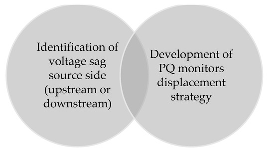
Figure 1.
Proposed classification model of the objectives of the related literature.
The works can be strictly classified into theoretical and practical [5]. This paper belongs to the group of practical works; and for its scope, the most important papers to cite are [15,35,36,37,38,39,40,41,42,43,44,45], i.e., those which are in the overlapping area of the Venn diagram (Figure 1). The theoretical papers [35,36,37,38,39,40,41,42] validate their approaches on test systems (IEEE schemes are the most commonly used; the Brazilian, CIGRÉ, and EPRI schemes are used occasionally), meanwhile in the practical studies [14,15,43,44,45], PQ monitoring campaigns are immediately begun without posterior self-reflection and criticism. The approaches of practical papers are significantly simpler than those of the theoretical papers; on the other hand, theoretical simulations are very limited and are not well prepared for implementation in practice. On the other hand, alternative approaches can hardly be imagined, thus applied methods remain the only option for the beginning. The limitations of the theoretical validation are described in detail in [5]: insufficient size (and therefore unclear adequacy in the case of real power systems), computational resources, required input (in particular, all node impedances, which can be very difficult to implement in practice), only the symmetrical faults are covered, topological flexibility, geographical compatibility (e.g., the difference between North American and European power systems), etc. Since PQ is a relatively recent research field [5,13], a deficit of exploitation experience has been noticed, along with the rules for allocation. At the moment, only two lemmas of PQ monitor observability have been used in [36,46]; however, since they are derived from Ohm’s law, the practical significance is diminished by the prerequisite for an entire grid model with impedance values. These lemmas are formulated as follows:
Lemma 1.
If voltage V1 of bus No. 1 is observable and current I12 of the line between buses No. 1 and No. 2 is observable, then voltage V2 of bus No. 2 is observable.
Lemma 2.
If voltage V12 through the line between buses No. 1 and No. 2 is observable, then current I12 of the line is observable.
Therefore, the need for simpler practical rules (principles, lemmas) regarding PQ monitor displacement along with voltage sag observability is obvious. In order to achieve this goal, the physical behavior of voltage sags must be investigated not only in a rational (analytical) way but also in an intuitive way. Occasionally, several investigation techniques can be found in the literature—for example, the voltage sag matrix (only for symmetrical faults) in [15,37,38,40,47] or the voltage–duration plane in [43,45]. In this paper, a full propagation path (including both TSO and DSO grids) will be monitored in the test grid—the chosen fragment of the Lithuanian power system which is a part of the post-Soviet BRELL ring. It can be regarded as a novel test system, because the analogous validation (i.e., BRELL-based) has not been found in the literature. This paper will cover all types of short-circuits and analyze them through the prism of both phase-to-phase and phase-to-ground voltages.
However, it is known a priori that the implementation of the above-mentioned task will not solve the fundamental economic problem to an adequate degree, i.e., will not sufficiently diminish a quantity of the devices. Therefore, additional criteria must be introduced: regardless of many available alternatives, the traditional subject—power supply reliability—is chosen to be the second criterion for the PQ monitor allocation strategy. Much political attention is devoted to reliability, for example, in [48,49,50]—the 5th, 6th and 7th CEER Benchmarking Reports—power supply interruptions are grouped into planned (outside the scope of this paper), unplanned, and unplanned excluding exceptional events (such as beforementioned Fukushima earthquake and tsunami). Despite being important, long-established and included into the main PQ standards (EN 50160:2010, IEEE Std 1159-2019, and others), the criterion almost cannot be met in the PQ monitor allocation literature, and is only briefly mentioned in [44,51]. The interconnection (possibly strong statistical correlation) between various reliability indexes and voltage sags should be expected (hypothesis)—in a similar manner to underground cables: according to the 5th Benchmarking Report [48] (pp. 39–40), which is also cited by the 7th [50] (p. 112), the correlation between total SAIDI (planned plus unplanned including exceptional events) and the percentage of underground cables in MV grids is 0.6 (and higher than 0.8 without Austria, Estonia, Finland, Poland, and Spain, i.e., with the data of 13 countries). The SAIDI calculation method along with other common indexes (SAIFI, MAIFI) are defined by IEEE Std 1366-2022 [52], and the duration (and, respectively consequences) after the sag/interruption depends on the settings and latency of protective relays and automation, in particular the undervoltage relay, automatic circuit recloser (ACR) and automatic transfer switch.
According to the modern literature [53,54], power system reliability is classified into two interdependent groups: (1) resource adequacy (a focus on power balance (e.g., peak demand, generation and transmission capacities, and operating reserves), which is outside the scope of this paper), and (2) operational reliability (a focus on the ability to withstand sudden disturbances). In spite of the fact that reliability is a matured research field and much information can be found in the classical literature [55,56], the interrelation between operational reliability and PQ has usually been unnoticed and skipped—the proposed concept is given in Figure 2. Possible reasons could be figured out from [5]: insufficient scientific and technical progress (because PQ is a relatively new research field), deficiency of massive PQ monitoring systems, absence of integration with other Smart Grid applications, mainly manual data processing, gaps in PQ law, a lack of unified assessment methods, and data confidentiality issues. The primary reasons for grid faults can be treated as another overlapping field, because they can cause both (i.e., either voltage sag or interruption), and the consequences depend on many factors—number of faulted phases, grid topology, relay protection and automation, the presence of mitigation devices, user criticality, etc. Currently, the probabilistic analysis (also forecasting) of PQ events (in particular, voltage sags/interruptions) along with their primary causes remains an open research field [5]. In spite of limited scientific literature, the latest paper [57] (2021) can be considered as the best and most relevant example. It investigates blackout history of the United States, and the Minnesota electrical grid’s resilience in 2009–2016 (in particular, the impact on SAIFI, CAIFI, and SAIDI) through a prism of primary causes (in particular, extreme weather conditions). The research became possible only after outage management system integration with an advanced metering infrastructure (about 24 thousand meters). In this paper, inspired by [57], the Lithuanian distribution grid will be investigated through a prism of both the primary causes and their correlation with reliability indexes (with available data for 2015–2018), which is important for a PQ monitor allocation strategy. Additionally, some information regarding grid equipment failure rates in Lithuania from 1995–2000, can be found in [56].

Figure 2.
Proposed interconnection model between power system reliability and power quality.
Considering the above, task No. 1 is to establish (investigate) the fundamental principles of voltage sags propagation and determine the universal rules of the optimization of their monitoring as much as is feasible in the created Lithuanian test grid. In addition, by implementing this task, a useful PQ database will be created as a secondary result for both manual voltage sag data analysis and further research through the application of AI. Task No. 2 is to establish (investigate) a supplementary criterion through a prism of primary reasons for voltage sag and (their correlation with) grid reliability indexes from data collected on the Lithuanian distribution grid. By combining both tasks, the main aim of this paper is to investigate the fundamental principles (rules) of voltage sags propagation and their interconnection with power supply reliability, which will have a high practical significance for PQ monitor allocation strategies.
2. Materials and Methods
2.1. Test Grid
The voltage sags propagation mechanism will be investigated with simulations in a test grid model created with MATLAB/Simulink. The scheme of the pseudo-realistic test grid is given in Figure 3: the chosen fragment of the Lithuanian power system is slightly (and realistically) expanded for research purposes. The Lithuanian power grid is a part of the post-Soviet BRELL ring where nominal voltage levels are as follows: HV—330 kV and 110 kV; MV—35 kV, 10 kV, and 6 kV; LV—0.4 kV. The test grid contains all possible voltage levels except 6 kV, both the TSO and DSO parts are included. The Lithuanian HV grid’s neutral is grounded via a separator (but some separators are disconnected to reduce short-circuit current ratios), the MV grid operates in isolated (or compensated) neutral mode, the LV grid’s neutral is grounded. The test grid contains the following oil-filled power transformers:
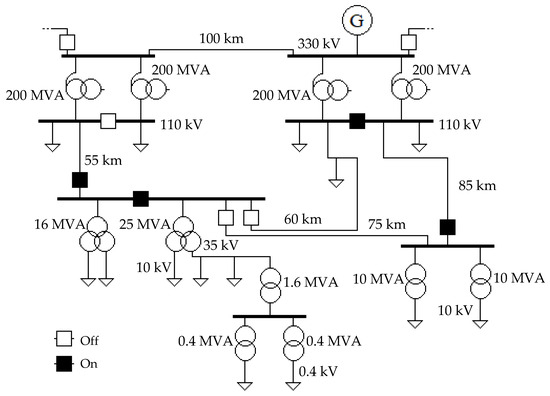
Figure 3.
The scheme of the test grid: the chosen fragment of the Lithuanian power system has been slightly (and realistically) expanded for the purposes of this research.
- Four 200 MVA 330/110 kV autotransformers. The common winding of an autotransformer is connected in wye with neutral point (Y0) [58]. The tertiary 10 kV winding supplies substation auxiliary transformer(s) and, in addition, some customers. Power rating of the tertiary winding is 40% (of 200 MVA), a delta configuration (Δ) is used in anticipation of zero sequence current harmonics [58,59];
- One 25 MVA 110/35/10 kV three-winding transformer. Power ratings of all windings are 100%. Noteworthily, in some cases, the rating of the secondary and (or) tertiary winding can be 67% [58]. Winding configuration can be either Y0/Δ/Δ-0-11, Y0/Δ/Δ-11-11, Y0/Y/Δ-0-11, or Y0/Δ/Y-11-0, etc.;
- One 16 MVA 110/35/10 kV three-winding transformer. Power ratings of all windings are 100% [58];
- Two 10 MVA 110/10 kV transformers. Winding configuration is Y0/Δ-11;
- One 1.6 MVA 35/10 kV transformer. Winding configuration is Y/Δ-11;
- Two 0.4 MVA 10/0.4 kV transformers. Winding configuration is Y/Y0-0.
The parameters of the power transformers are given in Appendix A: a part of them is given by the manufacturer, the rest must be calculated according to the described methodology. The values of those parameters are required for the equivalent circuits. Two-winding transformers are modeled with a T-type equivalent circuit where the magnetizing branch is connected in series. Noteworthily, the real physical behavior of a transformer can be represented better with the magnetizing branch being connected in parallel, however, it is more convenient to use the T-type model [58]. The task becomes more complicated in the case of the presence of both a three-winding transformer and an autotransformer. For power transmission line modeling, either the nominal Π-model or the distributed-element model can be used. See Appendix A for a detailed description. The lengths of the longest lines in the test scheme are specified in Figure 3. The longest length is 100 km. The test scheme contains only one power source. The commutators of other 330 kV power supply lines in the TSO grid are switched off. Initial topology of the grid is radial: some TSO circuit-breakers are switched off, thus the rings are not formed. Distributed generation is not included.
In the normal grid operation mode, the loading of a transformer is equal to 30–50%. In emergency mode, a 140% temporary overload is allowed [58,59]. Power consumption of auxiliary equipment in the substations is relatively small and equal to 50–500 kW [60]. In normal mode, it is realistically assumed that the average power factor is greater than 0.90, and the load imbalance is 0%. Voltage unbalance (imbalance) is assessed as the ratio of the negative sequence magnitude to the positive sequence, i.e., according to the definition given by EN 50160:2010 and IEEE Std 1159-2019. In this paper, the method of symmetrical components is used for voltage unbalance analysis (in particular asymmetrical faults). This complex linear transformation is expressed in the following way:
where: —three-phase voltage components; —the zero sequence component; —the positive sequence component; —the negative sequence component; —phasor rotation operator .
The information about both negative and zero sequence impedances can be found in [58,59]. In the case of transformers and power lines, the value of negative sequence impedance is equal to the positive sequence. In most cases, the zero sequence impedance of a transformer can be assumed to be approximately equal to the positive sequence. According to [59], the zero sequence impedance of an overhead power line can be 2–5.5 times higher than the positive sequence. The value depends on the tower structure—single-circuit, double-circuit, either one or two ground wires (also called “guard” wires). The zero sequence resistance of 110–330 kV overhead power lines is higher by 0.15 Ω/km [60].
2.2. Scenarios
As has been mentioned in Section 1, most voltage sags are caused by either short-circuit or an electric motor starting. In this research, only short-circuits will be investigated, covering all types of faults—three-phase, two-phase-to-ground, two-phase, and single-phase. The fault locations and potential monitoring sites are marked and numbered in Figure 4. It can clearly be seen that the majority of the nodes are included and will be investigated.
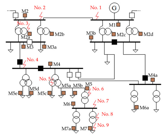
Figure 4.
The simulation scenarios and measurement nodes: fault locations are marked with red arrows, potential locations of PQ monitors—with brown squares.
The first four scenarios take place in the TSO grid: No. 1 is the beginning of the 330 kV 100 km line, No. 2—the end of the line, No. 3—the tertiary winding of the 200 MVA autotransformer, No. 4—the 110 kV busbar. The rest of the scenarios occur in the DSO grid: No. 5—the 10 kV winding of the three-winding transformer, No. 6—the end of the 35 kV line (i.e., the primary winding of the transformer), No. 7—the 10 kV busbar, No. 8—the beginning of the 0.4 kV grid (i.e., the secondary winding of the transformer), No. 9—the point of common coupling. Since the 110 kV circuit-breakers are open (see Figure 3), the test grid can be viewed as a grid with two radial branches—a left branch and a right branch—separated by a 100 km line. Monitors M1, M2, M3, M4, M5, M6, and M7 are placed along the longest branch—the main object of interest—where the majority of scenarios occur. The introduced terminology will be used in Section 3. Initially, the simulation is started in the normal operation mode with the grid of Figure 3 and the primary scenarios of Figure 4. Later, if additional questions arise, the research is supplemented with case studies.
2.3. Grid Reliability
For investigation of the primary reasons of grid faults (in particular voltage sags) and their impact on reliability indices, statistical data have been gathered in 2015–2018 during close collaboration with the Lithuanian DSO (“Energijos skirstymo operatorius”, AB), and classified according to voltage level and target group. The primary data will not be provided in detail due to confidentiality issues. Nevertheless, this issue will not be a considerable obstacle for the development of the allocation strategy. As has been mentioned before, due to the lack of analogous works regarding interconnection between PQ and reliability, our own/specific methodology must be developed considering the format (features) of available statistical data.
Reliability indexes for a distribution grid (in particular SAIFI and SAIDI) are calculated according to IEEE Std 1366-2022 by the following equations:
Both reliability indexes are calculated when (1) ACR events are included, and (2) not included. The proposal and investigation of such an approach has not been found in the literature. The following definition is proposed for ACR success evaluation through the prism of SAIDI:
where: —SAIDI is a superset of ACR events, i.e., ; —SAIDI is not a superset of ACR events, i.e., .
Theoretically, if all ACR performances are fully successful, the difference in numerator is equal to 0, and then success is equal to 1. However, it is hardly possible under real-life conditions (e.g., due to time settings of relay protection and automation, latency, incorrect logic, and device failure), hence at least a small influence (minutes of interruptions) is expected. A similar approach can be applied to SAIFI, which will estimate ACR event share. Obviously, both characteristics depend on fault location, grid topology, and level of automation. Since SAIFI is not related to duration, it can be used as a supplementary characteristic for a comparison of similar success values: the higher the ACR event part, the lower is their impact on SAIDI, and the more considerable ACR success is. The ratio through the prism of SAIFI is defined as follows:
Regression analysis is used for relationship estimation, and coefficients of a regression curve are determined using the least squares method. Model fitting is characterized by well-known coefficient of determination, which is generally defined as follows:
where: —sum of squares of residuals; —total sum of squares.
The second approach for ACR success evaluation is derived from the geometric meaning of a derivative at point :
where: —the regression function at point ; —slope (gradient) of the tangent line; —the angle between the tangent line and the axis of abscissas. The boundary conditions are the following: (1) when approaches the straight angle, then the reliability index is not influenced by the quantity of events; (2) when approaches the right angle, then the influence of a single event goes towards infinity. Mathematically this can be written as follows:
2.4. Probabilistic Analysis
In spite of the lack of literature regarding PQ event probabilities, it is clear that the research should be started with the Poisson distribution, which is usually used for event frequency assessment. The Poisson distribution is a discrete distribution whose probability mass function is:
where: —the expected value; —the number of occurrences.
On the other hand, since exact distribution types of specific event groups are often unknown, the alternatives should also be investigated. In the case of the Poisson distribution, the variance (of a random variable) is equal to . However, PQ data sets can have various variances and distributions, but according to the central limit theorem, in many situations, these distributions must tend towards the normal. Therefore, in addition, let us investigate the Gaussian distribution whose probability density function is:
where: —the mean; —the variance.
The second step is the confidence interval calculation. According to the conventional approach, when sample size is not fairly large, say lower than 40 [61], the central limit theorem does not apply, thus Student’s t-distribution must be used for the determination of the confidence interval:
where: —the mean; —the sample’s standard deviation; —sample size; —the t-test critical value, which depends on the test type (either one-tailed or two-tailed), significance level , and degrees of freedom which are determined as follows:
Standard deviation for a sample is calculated using the following formula:
where: —sample size; —sample mean.
It should be noted that the following properties of both the expected value and the variance are important to follow during data aggregation:
where: and are independent random variables.
In addition to the conventional approach, a more specialized method for the Poisson distribution mean will also be used, when the confidence interval is expressed as follows:
where: —the quantile function of chi-squared distribution; —the significance level (probability of a type I error); —observation from the Poisson distribution with mean [62]. The quantile function of the chi-squared distribution is:
where: —degrees of freedom; —the upper incomplete gamma function; —the gamma function.
Since the chi-squared distribution is a special case of the gamma distribution, Equation (16) is equivalent to:
where: —the quantile function of the gamma distribution; —the shape parameter; —the scale parameter equal to 1. The quantile function of the gamma distribution, when is equal to 1, is:
where: —the upper incomplete gamma function; —the gamma function.
The following expression of the interval can be derived by combining both approaches:
The final step is the comparison of the distributions. However, this is not an easy task; since the Gaussian distribution is continuous and the Poisson distribution is discrete, a continuity correction is required. The Poisson distribution can be approximated by the normal distribution the mean and variance of which is equal to . The approximation error determined by using the difference rule of integration:
where: and are real-valued functions. Since both areas are equal to 1, the percentage error can be implemented programmatically as follows:
where: —the array size; —the absolute error.
For the comparison of the distributions, we propose our own convolution-based method. The benefit of such a method is that convolution evaluates the overlapping of function shapes (areas), considering all values of the shift. The convolution of two functions is given by:
where: and are non-negative real-valued functions. Convolution is commutative. Please note that the above-used symbol need not represent the time domain.
Discrete convolution is given by:
Convolution of both density functions is compared to the autoconvolution (i.e., convolution of a function with itself) of both functions, and, respectively two errors are obtained: in this work, the absolute error is calculated. Noteworthily, the squared error can also be used: the difference is that the squared error heavily weights outliers (i.e., large errors). Hence, the similarity criteria are defined as follows:
The nearer and are to 0, the higher the similarity is between both distributions. In this paper, for a better explanation/intuition, both and will be given. On the other hand, the final similarity criteria can be defined by:
In some cases, two-dimensional probabilistic analysis is possible. The definition of a conditional probability is the following:
where: and are dependent events.
In this paper, the Weibull, gamma, and beta distributions will be used (examined) for assessment. All of them are continuous distributions. The probability density function of the Weibull distribution is:
where: —the shape parameter; —the scale parameter.
The probability density function of the gamma distribution is:
where: —the shape parameter; —the scale parameter; —the gamma function.
The probability density function of the beta distribution is:
where: —the shape parameter; —the shape parameter; —the gamma function.
3. Results
The first part of the paper—the investigation of the voltage sags propagation mechanism—is given in Section 3.1. The second part—the investigation of the primary causes and reliability indexes in the Lithuanian DSO grid—is given in Section 3.2.
3.1. Voltage Sag Matrix
The idea of a voltage sag matrix has been inherited from [15,37,38,40]; however, only the case of a symmetrical fault has been found. In this paper, a voltage sag matrix will be introduced for asymmetrical faults too, i.e., two-phase-to-ground (Section 3.1.2), two-phase (Section 3.1.3), and single-phase (Section 3.1.4). For these cases, the following modifications must be applied: the cells of the matrix must be a row vector with three entries, and phase-to-phase and phase-to-ground sags must be analyzed with separate matrixes.
The terminology used for voltage sag characterization usually is confusing [1]. At present, assessment methods of many PQ events lack a universally unified (agreed) approach [5]. Short-duration RMS variation is not an exception: the reference voltage for the assessment of both voltage sags and swells remains an open question. The following options are available: (1) nominal grid voltage, (2) nominal voltage of transformer windings, (3) pre-fault voltage (Figure 5), and (4) residual voltage. The choice depends on the objective: for example, impact on grid equipment, impact on end-user equipment, legal disputes, determination of settings for relay protection and automation, database for machine learning, classification and situation assessment, etc.
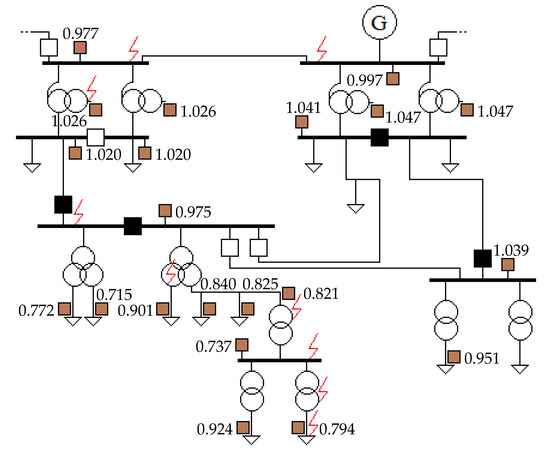
Figure 5.
Pre-fault voltages (p.u.) of the test grid in normal operation mode. During the load-flow study, the loads impedances were constant.
In this paper, voltage sag matrixes are filled in with residual voltage values expressed in per-unit system (when the reference is the nominal grid voltage). In addition, the following color-coding is used for the analysis from another angle: the dark green color denotes that a fault has no impact on voltage level (when the reference is pre-fault voltage); light green—the impact is not higher than −10% (i.e., within the boundaries of rapid voltage change (RVC), when the reference is pre-fault voltage); red—residual voltage is equal to 0.1 p.u. (the reference is the nominal grid voltage); orange—a case of severe voltage sag when residual voltage is 0.2–0.4 p.u. (the threshold is set according to the sag classification table given in EN 50160:2010, the reference is the nominal grid voltage); yellow—the rest of voltage sags whose depth is approximately equal to 20–60% (when the reference is pre-fault voltage); white (no color)—voltage swell (including the boundaries of RVC, when the reference is pre-fault voltage). In the case of voltage swells, the color-coding has not been applied because a sag and a swell of the same percentage will have different effects on grid equipment. Nominal grid voltages are given in Figure 3, nominal voltages of transformer windings in Appendix A. Pre-fault voltage values in normal operation mode are given in Figure 5. Please note that tap changers are used for voltage regulation (nominal voltages of transformer windings are given in Appendix A), but reactive power compensators are not included, hence a voltage drop in some nodes is higher than 10–15%. The issue will not affect the results of this research, but it must be considered for error elimination during the estimation of the level of short-duration RMS variations.
In all scenarios, the simulation sampling time is 10−6 s, stop time is 0.16 s, faults occur at 0.06 s after the start of the simulation. Besides, in MATLAB/Simulink, computational time also depends on the quantity of scopes. The simulation of each scenario took up to 5 min (the base frequency of the 4-core processor is 2.30 GHz, RAM—6.00 GB).
3.1.1. Three-Phase Fault
Three-phase short-circuit is the rarest and the most severe fault, also the simplest to investigate due to the symmetry. In Table 1, Table 2 and Table 3, residual voltages (p.u.) are given: the monitor number (according to Figure 4) with its pre-fault voltage (according to Figure 5) are given in the first two columns, the fault location (i.e., corresponding monitor number according to Figure 4) with the scenario in the brackets (respectively) is given in the first rows. The voltages of the fault nodes are underlined. Scenario No. 8 does not have an assigned monitor. Results are also given in the figures (starting from Figure 6): voltage in volts is given in the ordinate axis, and time in seconds is given in the abscissa axis.

Table 1.
Three-phase fault voltage sag matrix of the nodes of direct interest.
Table 2.
Three-phase fault voltage sag matrix of the rest of the nodes.
Table 3.
Three-phase fault voltage sag matrix of the right branch.
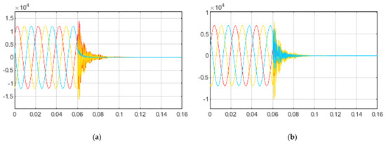
Figure 6.
Scenario No. 2, three-phase fault. (a) Phase-to-phase voltage of M5c; (b) Phase-to-ground-voltage of M5c.
Deep investigation of Scenario No. 1 is not required: it is obvious that a three-phase short-circuit at the terminals of the only generator will cause supply interruption at each node in the test grid. When the short-circuit occurs at the end of the 330 kV 100 km line (Scenario No. 2), the interruptions are observed in all following nodes of the left branch (Figure 6) and are not observed in the generator’s busbar and the following nodes of the right branch. There, in the right branch, the dangerous PQ events—oscillatory transients—appear (Figure 7 and Figure 8), which once more supports the affirmation, given by [5] (p. 19), that PQ events are strongly interconnected. Please note that the event cannot be classified as notching ringing, since according to IEEE Std 1159-2019, notching is “a periodic waveform disturbance caused by normal operation of power electronic devices.”

Figure 7.
Scenario No. 2, three-phase fault. (a) Phase-to-phase voltage of M1; (b) Phase-to-ground-voltage of M1.

Figure 8.
Scenario No. 2, three-phase fault. (a) Phase-to-phase voltage of M2d; (b) Phase-to-ground-voltage of M2d.
Since electric generators are (an effective) measure for voltage sag mitigation (as mentioned in Section 1), the first additional question arises: what is the dependence between the length of the 330 kV line and the residual voltage of M1. The results are given in Figure 9: the sag threshold (0.9 p.u.) is reached when the distance is approximately equal to 20 km, and the dependence can be approximated with a natural logarithm model (with a very high coefficient of determination). Since a three-phase fault is the most severe fault, it is the easiest fault to detect. The opposite boundary condition is a single-phase fault (see Section 3.1.4): in this case, the threshold is 10 km (Figure 10). The line is modeled as a distributed-parameter line (see Appendix A).

Figure 9.
Scenario No. 2, three-phase fault. The dependence between the length of the 330 kV line and the residual voltage of M1.
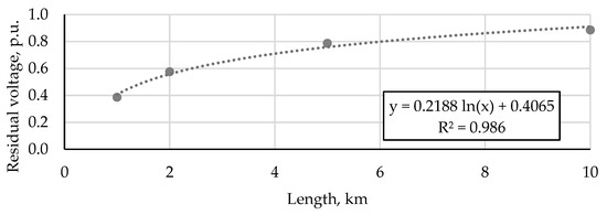
Figure 10.
Scenario No. 2, single-phase fault. The dependence between the length of the 330 kV line and the phase-to-ground residual voltage of the faulted phase of M1.
The short-circuit at the autotransformer’s tertiary winding (Scenario No. 3) causes a power supply interruption (0.1 p.u.) in all nodes of the left branch, including both the primary and secondary windings of the autotransformer (Figure 11). Analogously to Scenario No. 2, transients are observed in the right branch (Figure 12). At this point, the second additional question arises about the propagation path when the fault location (node) is shifted from the tertiary winding (along the same 10 kV line) by 0.5–1 km (modification of Scenario No. 3). The results are given in Figure 13: when the distance is increased by 0.5 km, the fault does not propagate against the power-flow and does not affect the autotransformer windings. The last fault of the TSO grid occurs at the 110 kV busbar (Scenario No. 4). Similarly, the sag does not propagate against the power-flow (Figure 14), i.e., from M4 to M3.
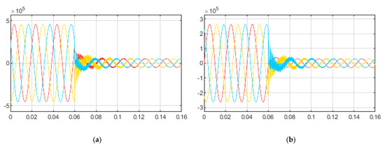
Figure 11.
Scenario No. 3, three-phase fault. (a) Phase-to-phase voltage of M2; (b) Phase-to-ground-voltage of M2.
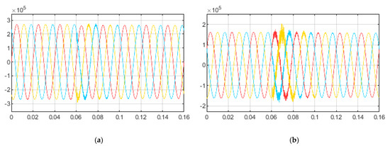
Figure 12.
Scenario No. 3, three-phase fault. (a) Phase-to-phase voltage of M1; (b) Phase-to-phase-voltage of M4a.

Figure 13.
Modification of scenario No. 3, three-phase fault. (a) Phase-to-phase voltage of M2a, when the distance to the fault is 1 km; (b) Phase-to-phase-voltage of M2a, when the distance to the fault is 0.5 km.
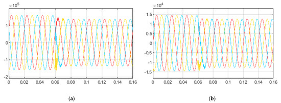
Figure 14.
Scenario No. 4, three-phase fault. (a) Phase-to-phase voltage of M3; (b) Phase-to-phase voltage of M2b.
Let us investigate the topological changes of the HV grid and begin with power-flow directions (Figure 15). The green arrows indicate the directions of power-flow in normal operation mode, and the directions remain the same in all three possible configurations (i.e., when either both circuit-breakers are closed or any one of them is closed). In fault mode, power always flows towards the short-circuit location. In Figure 15, the red arrows point in the direction of power-flow during Scenario No. 10, when both circuit-breakers are closed. When the directions of power-flow are known, the analysis of voltage sags propagation becomes easier. In the case of Scenario No. 2, when the voltage of M3 remains equal to zero, the circuit-breakers have the following influence:
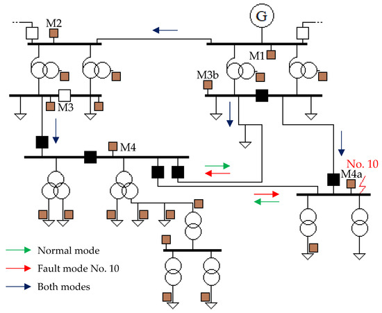
Figure 15.
Power-flow directions in TSO grid when the both circuit-breakers lockout the rings in the case of the normal mode and the fault mode of Scenario No. 10. During the load flow-study, the loads impedances were constant.
- When the circuit-breaker between M3b and M4 is closed, the power-flow from the right branch supports the busbar of M4, thus the voltage in the 110 kV busbar of M4 is equal to 0.4 p.u. (Figure 16a). Since the line is sufficiently long (60 km), only transients without sags are observed on the right side (similar to the radial grid case).
 Figure 16. Modifications of Scenario No. 2, three-phase fault. (a) Phase-to-phase voltage of M4, when the circuit-breaker between M3b and M4 is closed; (b) Phase-to-phase voltage of M4a, when both circuit-breakers are closed.
 - If both circuit-breakers are closed, the interruption at the 110 kV busbar of M4 is also avoided and the voltage is even higher (0.5 p.u.); however, in contrast to the previous configuration, the sag is also felt by M4a (Figure 16b).
In the opposite case, when the short-circuit occurs at M4a (Scenario No. 10), the circuit-breakers have the following influence:
- When both circuit-breakers are closed, the voltage of the dependent M4 is equal to 0.7 p.u. (Figure 17a), while the voltage of M4a is obviously equal to 0.
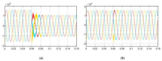 Figure 17. Scenario No. 10, three-phase fault. (a) Phase-to-phase voltage of M4, when both circuit-breakers are closed; (b) Phase-to-phase voltage of M4, when the circuit-breaker between M3b and M4 is closed.
 - When the (direct) circuit-breaker between M4 and M4a is closed, the voltage of M4 is lower and equal to 0.5 p.u., due to the absence of direct support from the right side (see power-flow direction in Figure 15).
- When the direct circuit-breaker is open, the electrical distance between the busbars is sufficiently increased, the circuit-breaker between M3b and M4 does not affect the situation (Figure 17b).
To sum up, in a general case, ring formations are useful for line current reduction (according to Kirchhoff’s current law), and, in a specific case—for voltage sag mitigation (interruption avoidance) in some nodes. On the other hand, circuit-breakers reduce electrical length between busbars, and hence the interdependence and vulnerability of these connected busbars is increased. The solution, i.e., acceptable configuration, depends on the specific circumstances, for example, the criticality (or vulnerability) of end-user equipment or the presence of generators. However, the preferred configuration can be determined only in particular cases, since the optimization of an entire transmission grid is hardly expected due to the large variety of possible configurations. Noteworthy, the topological analysis (at least partial) is rarely found in the PQ literature (even in small test systems), which indicates the poor flexibility of the proposed approaches and algorithms [5].
Let us continue with the faults in the distribution grid. In Scenario No. 5, the short-circuit (which occurs at the 10 kV winding of the three-winding transformer) almost does not propagate upwards, i.e., is felt only at the primary winding within the limits of RVC (Figure 18), and the transients are not observed. The fault propagates downwards: the interruption is observed in both the 35 kV and 10 kV windings of the transformer.
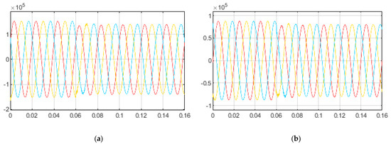
Figure 18.
Scenario No. 5, three-phase fault. (a) Phase-to-phase voltage of M4; (b) Phase-to-ground-voltage of M4.
In Figure 19, Figure 20 and Figure 21, voltages in the MV grid are given when the fault occurs at the primary winding of the 35/10 kV transformer (Scenario No. 6). The short-circuit has no impact on the HV side (Figure 22). In Scenario No. 7, the distance between the fault location and the 35/10 kV transformer is 10 km: analogously to Scenario No. 5, in the 35 kV grid, the fault is felt within the limits of RVC (Figure 23).
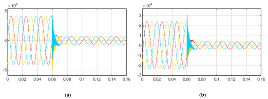
Figure 19.
Scenario No. 6, three-phase fault. (a) Phase-to-phase voltage of M5b; (b) Phase-to-ground-voltage of M5b.
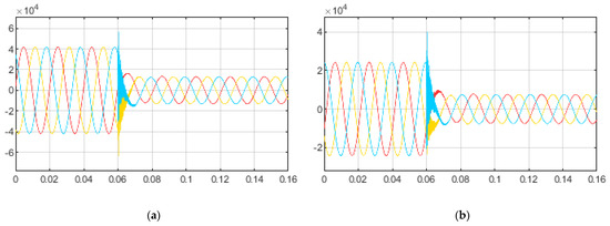
Figure 20.
Scenario No. 6, three-phase fault. (a) Phase-to-phase voltage of M5a; (b) Phase-to-ground-voltage of M5a.
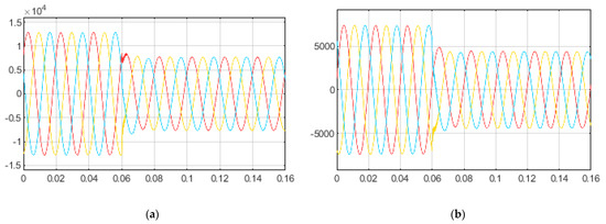
Figure 21.
Scenario No. 6, three-phase fault. (a) Phase-to-phase voltage of M5c; (b) Phase-to-ground-voltage of M5c.

Figure 22.
Scenario No. 6, three-phase fault. (a) Phase-to-phase voltage of M4; (b) Phase-to-ground-voltage of M4.
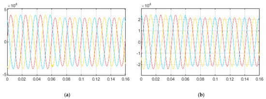
Figure 23.
Scenario No. 7, three-phase fault. (a) Phase-to-phase voltage of M5; (b) Phase-to-ground-voltage of M5.
The rest of the scenarios occur in the LV grid. When the fault occurs at the secondary winding of the 10/0.4 kV transformer (Scenario No. 8), the impacts on the 10 kV and 35 kV sides are shown in Figure 24; impact on the neighboring 0.4 kV line in Figure 25. When the fault occurs at the point of common coupling (Scenario No. 9), the sag depth at the beginning of the 0.4 kV line is only 20%, which could be eliminated with the help of distributed generators. Similar voltage sags are observed in the 10 kV line and the neighboring line (Figure 26).
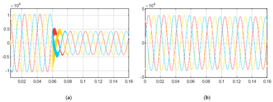
Figure 24.
Scenario No. 8, three-phase fault. (a) Phase-to-phase voltage of M6; (b) Phase-to-phase voltage of M5.
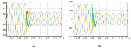
Figure 25.
Scenario No. 8, three-phase fault. (a) Phase-to-phase voltage at the beginning of the 0.4 kV line of M7a; (b) Phase-to-ground-voltage at the beginning of the 0.4 kV line of M7a.
Figure 26.
Scenario No. 9, three-phase fault. (a) Phase-to-ground voltage of M6; (b) Phase-to-ground voltage at the beginning of the 0.4 kV line of M7a.
3.1.2. Two-Phase-to-Ground Fault
The research is continued with asymmetrical short-circuits, starting from a two-phase-to-ground fault. As has been mentioned before, the investigation of asymmetrical faults has not been found in the literature, where the voltage sag matrix has been applied only in the case of three-phase faults. The asymmetrical case is different: voltages must be analyzed separately with two interdependent voltage sag matrixes—phase-to-phase (Table 4) and phase-to-ground (Table 5). The fault occurs between phase A, phase B, and the ground. In this paper, the cells of asymmetrical fault matrixes are filled in the following order (red, yellow, blue curves): phase-to-phase—AB, AC, BC, phase-to-ground—A, B, C.
Table 4.
Two-phase-to-ground fault phase-to-phase voltage sag matrix.
Table 5.
Two-phase-to-ground fault phase-to-ground voltage sag matrix.
Analogously to the previous case, the short-circuit at the generator’s terminals (Scenario No. 1) spreads out to all nodes. In Scenario No. 2, the fault has no impact on the voltage level of the generator’s busbar and the right branch, but distorts their voltage waveforms (Figure 27).

Figure 27.
Scenario No. 2, two-phase-to-ground fault. (a) Phase-to-phase voltage of M1; (b) Phase-to-ground voltage of M1.
Let us begin with the upstream propagation. The following principle is observed in the case of both of the severest faults (Table 1, Table 2, Table 3, Table 4 and Table 5): if the fault location is not transformer’s secondary (tertiary) winding, it does not propagate upwards (to the primary winding), and the maximal effect is within the boundaries of RVC (except Scenario No. 4 in Table 5, when the depth of phase-to-ground voltage sag at M2 is slightly larger—up to 20%). However, in the case of the two-phase-to-ground fault, in spite of the green-colored cells, voltage unbalances (both phase-to-phase and phase-to-ground) are observed at these nodes. For example: (1) when the fault occurs at M6 (Scenario No. 7), the unbalance is seen at M5 (Figure 28a); (2) when the fault occurs at M7 (Scenario No. 9), the unbalance is seen at M6 (Figure 28b).
Figure 28.
(a) Scenario No. 7, two-phase-to-ground fault, phase-to-phase voltage of M5; (b) Scenario No. 9, two-phase-to-ground fault, phase-to-phase voltage of M6.
In the case of Scenario No. 4, when the fault occurs at M4 (55 km from the autotransformer), the unbalance is felt not only at the primary winding of the autotransformer, but also at the secondary (Figure 29) and tertiary windings (Figure 30).
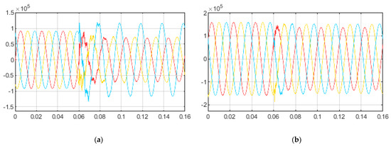
Figure 29.
Scenario No. 4, two-phase-to-ground fault. (a) Phase-to-phase voltage of M3; (b) Phase-to-ground voltage of M3.
Figure 30.
Scenario No. 4, two-phase-to-ground fault. (a) Phase-to-phase voltage of M2a; (b) Phase-to-ground voltage of M2a.
Considering the above, the interconnection of two-phase-to-ground short-circuits with the unbalance seems to be a promising basis for the voltage sag identification task (see Section 1). Moreover, downstream sags could be identified only with protective relays (and smart meters—to determine whether the negative sequence unbalance is caused by consumers), i.e., without PQ monitors; however, currently, the interconnection patterns of symmetrical components have not been comprehensively examined. Scenario No. 4 patterns (Table 6) can be given as an example. The fault at the end of the 110 kV line (M4) affects not only the autotransformer’s 110 kV winding (M3), but also the rest of the windings—the 330 kV (M2) and the 10 kV (M2a): for example, a 6.2% negative sequence phase-to-phase unbalance is observed at M2. Symmetrical component propagation from M4 (the fault node) along the 110 kV line to M3 is given in Figure 31. Please note that this research of symmetrical components is beyond the scope of EN 50160:2010 (because it regulates only negative sequence magnitude).
Table 6.
Symmetrical components of both voltages of M4 and the rest of the upward monitors, after the two-phase-to-ground fault at M4 (Scenario No. 4).
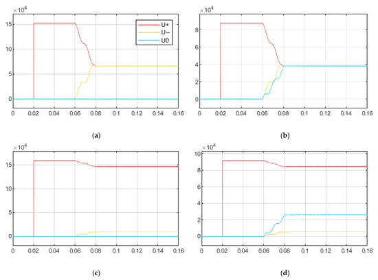
Figure 31.
Scenario No. 4, two-phase-to-ground fault. (a) Symmetrical magnitudes of phase-to-phase voltage of M4; (b) Symmetrical magnitudes of the phase-to-ground voltage of M4; (c) Symmetrical magnitudes of the phase-to-phase voltage of M3; (d) Symmetrical magnitudes of phase-to-ground voltage of M3.
Next, contrary to the symmetrical case, non-identical propagation patterns are seen in Table 4 and Table 5—the rotation is observed among the interruption, sag, swell, and RVC events in both directions. The example of the dependence of upward voltage patterns on winding configuration is given in Figure 32: when a two-phase-to-ground fault occurs at the end of the 35 kV line (Scenario No. 6), the voltage at M5a is similar in all cases (Figure 33), but the voltage at M5c is not (Figure 34 and Figure 35).
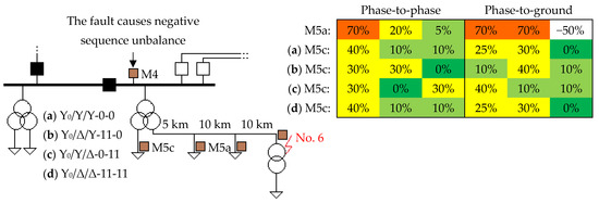
Figure 32.
Three-winding transformer configuration influence on upward voltage patterns (voltage sag depth at M5a and M5c), after the two-phase-to-ground fault at M5 (Scenario No. 6).
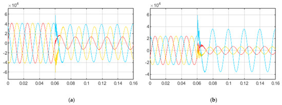
Figure 33.
Scenario No. 6, two-phase-to-ground fault. (a) Phase-to-phase voltage of M5a; (b) Phase-to-ground voltage of M5a.
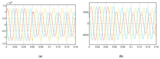
Figure 34.
Scenario No. 6, two-phase-to-ground fault. (a) Phase-to-phase voltage of M5c, when the winding configuration is Y0/Y/Δ-0-11; (b) Phase-to-ground voltage of M5c, when the winding configuration is Y0/Y/Δ-0-11.
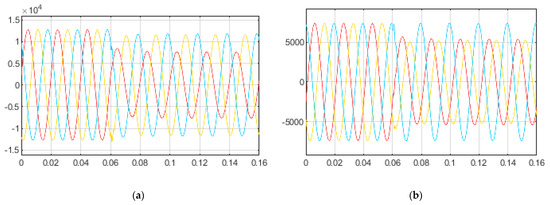
Figure 35.
Scenario No. 6, two-phase-to-ground fault. (a) Phase-to-phase voltage of M5c, when the winding configuration is Y0/Y/Y-0-0; (b) Phase-to-ground voltage of M5c, when the winding configuration is Y0/Y/Y-0-0.
In the case of the LV grid, the upward propagation mechanism is as follows: (1) if a fault occurs at the secondary winding of the 10/0.4 kV transformer (Scenario No. 8), voltage sags are observed in both the 10 kV and 35 kV grids (Figure 36a), and also (obviously) in the neighboring 0.4 kV line; (2) if the distance between the fault and the secondary winding is, for example, 1 km (Scenario No. 9), only a voltage unbalance is caused in both the 10 kV busbar (Figure 28b) and the neighboring 0.4 kV line (Figure 36b), i.e., voltage sag does not propagate upwards.
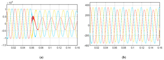
Figure 36.
(a) Scenario No. 8, two-phase-to-ground fault, phase-to-phase voltage of M6; (b) Scenario No. 9, two-phase-to-ground fault, phase-to-phase voltage at the beginning of the 0.4 kV line of M7a.
Non-uniform patterns are also noticed in the downstream propagation path. In the case of Scenario No. 1, transition M5–M6 (Figure 37 and Figure 38) can be given as an example. Another example can be related to downward propagation through the autotransformer—path M2–M2a–M3 in the case of either Scenario No. 1 or No. 2. The patterns do not coincide (correlate) with the upward propagation path, in particular, through the three-winding transformer (e.g., the case in Figure 32): for example, compare voltage at M2 in the case of Scenarios Nos. 1–3, or M5 in the case of Scenarios No. 4 and No. 5.
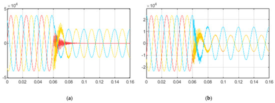
Figure 37.
Scenario No. 1, two-phase-to-ground fault. (a) Phase-to-phase voltage of M5; (b) Phase-to-ground voltage of M5.
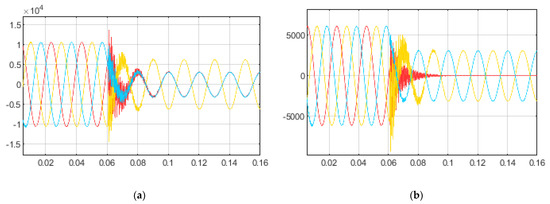
Figure 38.
Scenario No. 1, two-phase-to-ground fault. (a) Phase-to-phase voltage of M6; (b) Phase-to-ground voltage of M6.
Fault node patterns (Table 7) also vary and depend on short-circuit location (see Table 4 and Table 5). At a two-phase-to-ground fault location, the voltage swell’s magnitude range is 110–150% of the pre-fault level. Usually, voltage swells do not propagate downwards through a transformer (except Scenario No. 2), but obviously have a high negative impact, for example, on transmission tower insulators. The highest voltage swells (1.8–2.0 p.u.) have been noticed at M3 and M4 (Figure 39) in Scenario No. 2.
Table 7.
Voltage sag depth dependence on two-phase-to-ground fault location.
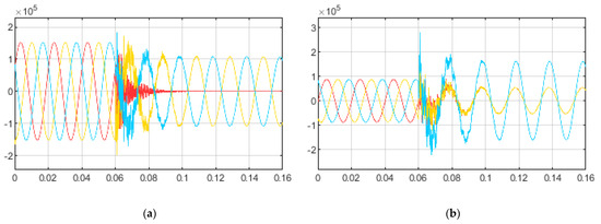
Figure 39.
Scenario No. 2, two-phase-to-ground fault. (a) Phase-to-phase voltage of M4; (b) Phase-to-ground voltage of M4.
3.1.3. Two-Phase Fault
Another type of asymmetrical fault is the two-phase short-circuit. The fault occurs between phase A and phase B. Voltage sag matrixes are given in Table 8 and Table 9.
Table 8.
Two-phase fault phase-to-phase voltage sag matrix.
Table 9.
Two-phase fault phase-to-ground voltage sag matrix.
The comparison of Table 8 and Table 9 with two-phase-to-ground matrixes (Table 4 and Table 5) reveals that the residual voltages of two-phase faults are higher, and voltage swells are not observed since there is no (direct) contact with the ground. Contrary to the two-phase-to-ground case (Table 7), two-phase fault patterns almost do not depend on the short-circuit location (Table 10). On the other hand, a high degree of similarity can be noticed in the downstream propagations, for example, comparing voltages at M2 (Figure 40 and Figure 41) of Scenario No. 1.
Table 10.
Voltage sag depth dependence on two-phase fault location.

Figure 40.
Scenario No. 1, two-phase fault. (a) Phase-to-phase voltage of M2; (b) Phase-to-ground-voltage of M2.

Figure 41.
Scenario No. 1, two-phase-to-ground fault. (a) Phase-to-phase voltage of M2; (b) Phase-to-ground voltage of M2.
When a two-phase fault occurs at HV level (Scenarios No. 1, No. 2, and No. 4), the impact on two phase-to-ground voltages of both the 10 kV and 0.4 kV grid (Figure 42) is within the limits of RVC, which means that the majority of single-phase equipment will not be affected. Meanwhile, voltage sag patterns in the 330 kV, 110 kV, and 35 kV grids are similar to those of the fault node (Table 10). The same effect on the LV grid is observed in Scenario No. 6. Conversely, when a fault occurs at the transformer’s tertiary winding (Scenarios No. 3 and No. 5), patterns rotate (i.e., patterns are similar to, for example, the voltages of both M3 and M4 in the case of Scenarios No. 1 and No. 2, or M5 in the case of Scenarios No. 1, No. 2, and No. 4): two phase-to-ground voltage sags are caused, while the third phase remain healthy (Figure 43).
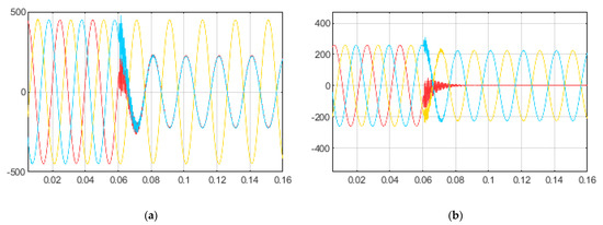
Figure 42.
Scenario No. 2, two-phase fault. (a) Phase-to-phase voltage of M7; (b) Phase-to-ground-voltage of M7.
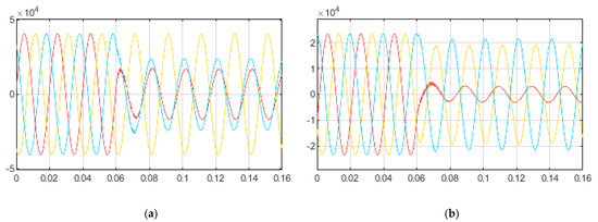
Figure 43.
Scenario No. 3, two-phase fault. (a) Phase-to-phase voltage of M5; (b) Phase-to-ground-voltage of M5.
Upward propagation mechanisms of two-phase and two-phase-to-ground faults have many similarities. For example, similar to the two-phase-to-ground case, when a two-phase short-circuit occurs at M4 (Scenario No. 4), the voltage unbalance is observed at M2 (Figure 44), also at M2a, M2b, and M3a. If a fault occurs at the primary winding of the 35/10 kV transformer (Scenario No. 6), it affects the 110/35/10 kV transformer’s tertiary winding (Figure 45). If a two-phase short-circuit occurs at the end of the 10 kV 10 km line (Scenario No. 7), voltage sags are observed at the beginning of the line (Figure 46), but only a negative sequence unbalance is observed at the 35/10 kV transformer’s primary winding (Figure 47). A short-circuit at the secondary winding of the 10/0.4 kV transformer (Scenario No. 8) is fully felt by both M6 and M7a (Figure 48). Conversely, if the distance from the secondary winding is increased by 1 km (Scenario No. 9), only the voltage unbalance is observed at both M6 and M7a (Figure 49).
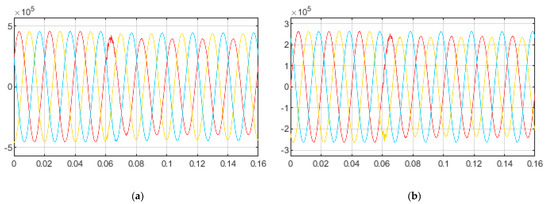
Figure 44.
Scenario No. 4, two-phase fault. (a) Phase-to-phase voltage of M2; (b) Phase-to-ground-voltage of M2.
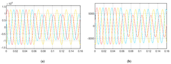
Figure 45.
Scenario No. 6, two-phase fault. (a) Phase-to-phase voltage of M5c; (b) Phase-to-ground-voltage of M5c.
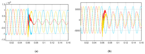
Figure 46.
Scenario No. 7, two-phase fault. (a) Phase-to-phase voltage at the beginning of the 10 kV line of M6; (b) Phase-to-ground-voltage at the beginning of the 10 kV line of M6.

Figure 47.
Scenario No. 7, two-phase fault. (a) Phase-to-phase voltage of M5; (b) Phase-to-ground-voltage of M5.
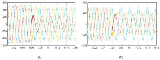
Figure 48.
Scenario No. 8, two-phase fault. (a) Phase-to-phase voltage of M7a; (b) Phase-to-ground-voltage of M7a.
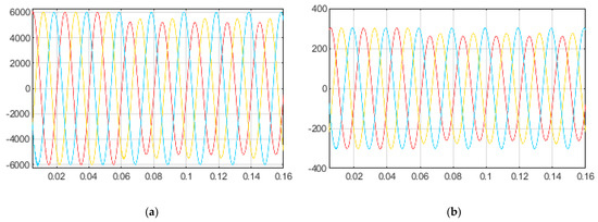
Figure 49.
Scenario No. 9, two-phase fault. (a) Phase-to-ground voltage of M6; (b) Phase-to-ground-voltage of M7a.
3.1.4. Single-Phase Fault
The last type of asymmetrical fault—the single-phase short-circuit—causes the lightest damage to the grid. For this reason, due to the shortest propagation path, fault detection is the most difficult. Voltage swells are characteristic for this type of fault, similar to the case of a two-phase-to-ground short-circuit. The fault occurs between phase A and the ground. Voltage sag matrixes are given in Table 11 and Table 12.
Table 11.
Single-phase fault phase-to-phase voltage sag matrix.
Table 12.
Single-phase fault phase-to-ground voltage sag matrix.
The single-phase fault pattern depends on neutral mode and electrical distance from the power source (Table 13). Voltage swells are not observed when the short-circuit occurs at the generator’s busbar (Figure 50). At the fault node, the lowest voltage swell magnitudes are typical for an HV grid (if compared with either an MV or an LV). A typical fault node pattern in distribution grids (10 kV) is given in Figure 51: contrary to the HV grid, the fault does not affect phase-to-phase voltage when it occurs in either an MV or an LV grid (except Scenario No. 5). Despite being the most common fault in overhead power lines, the operator will almost always avoid legal responsibility. For a three-wire system, EN 50160:2010 requires only phase-to-phase voltage to be taken into consideration; however, it is obvious that phase-to-ground events are also harmful for grid equipment (in particular voltage swells for insulation). On the other hand, single-phase faults, which occur in an MV grid (Scenarios Nos. 5–7), do not interrupt end-users on the LV side, and for this reason, this is the longest-lasting fault. The disconnection of a short-circuited line along with other required commutations is initiated only after the discovery of the fault location by electricians (e.g., after a few hours).
Table 13.
Voltage sag depth dependence on single-phase fault location.
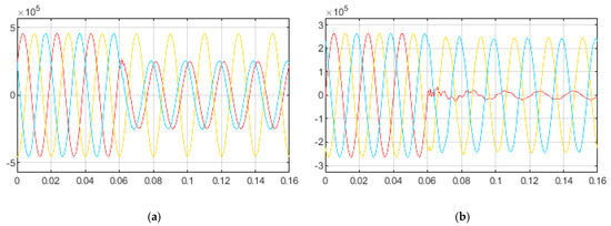
Figure 50.
Scenario No. 1, single-phase fault. (a) Phase-to-phase voltage of M2; (b) Phase-to-ground-voltage of M2.
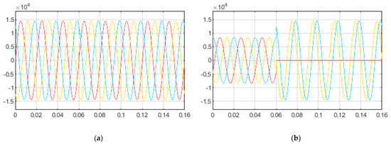
Figure 51.
Scenario No. 3, single-phase fault. (a) Phase-to-phase voltage of M2a; (b) Phase-to-ground voltage of M2a.
Single-phase faults in the TSO grid are more dangerous. In the case of Scenarios No. 1, No. 2, and No. 4, when the fault occurs in an HV grid, downstream penetration into an LV grid is stronger than in the case of Scenarios Nos. 5–7 (see Table 11 and Table 12). For example, a single-phase fault at the primary winding of the 35/10 kV transformer (Scenario No. 6) does not propagate even to the 10 kV grid (Figure 52), but the fault at the 110 kV busbar (Scenario No. 4), given in Figure 53, reaches both sides—the MV grid (Figure 54) and consequently the LV grid. On the other hand, contrary to all previous types of faults, the propagation path mitigates the consequences by itself—many residual voltage gains (in particular conversion from voltage interruption to sag) can be seen in Table 12. In the case of Scenario No. 4, transition from M4 to M5 can be given as an example: the degree of phase-to-ground voltage unbalance at M5, which is caused by the fault at M4 (Figure 53b), is sufficiently enhanced (Figure 54b).
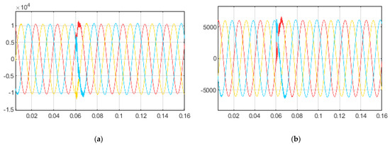
Figure 52.
Scenario No. 6, single-phase fault. (a) Phase-to-phase voltage of M6; (b) Phase-to-ground voltage of M6.
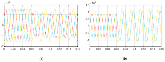
Figure 53.
Scenario No. 4, single-phase fault. (a) Phase-to-phase voltage of M4; (b) Phase-to-ground voltage of M4.
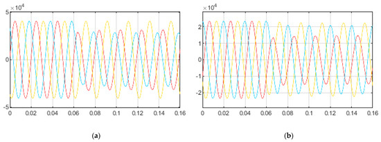
Figure 54.
Scenario No. 4, single-phase fault. (a) Phase-to-phase voltage of M5; (b) Phase-to-ground voltage of M5.
Upstream propagation of single-phase faults is considerably weaker. Contrary to the previous cases, the single-phase sag usually does not propagate upwards through a transformer, even if it occurs at the secondary winding. In Scenarios No. 8 and No. 9, the faults (Figure 55) not only do not propagate to the neighboring 0.4 kV line, but also do not cause any voltage unbalance at M6 and consequently M7a (Figure 56).

Figure 55.
(a) Scenario No. 8, single-phase fault, phase-to-ground voltage of M7; (b) Scenario No. 9, single-phase fault, phase-to-ground voltage of M7.
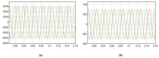
Figure 56.
Scenario No. 8, single-phase fault. (a) Phase-to-ground voltage of M6; (b) Phase-to-ground voltage of M7a.
In Scenario No. 4, despite the fact that the unbalance is decreasing upwards (across the 110 kV line), it is observed at the primary winding of the autotransformer (Figure 57 and Figure 58). The propagation of symmetrical components from M4 to M2 is given in Figure 59: the negative sequence phase-to-phase unbalance at M2 is 4.9%, the phase-to-ground is 2.5%. These values (especially for the 330 kV grid) are high, because the limit on negative sequence unbalance in EN 50160:2010 (which is applicable up to 110 kV) is 2–3%.
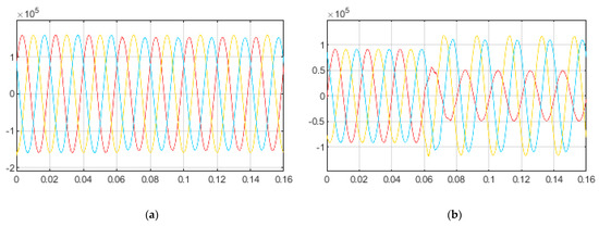
Figure 57.
Scenario No. 4, single-phase fault. (a) Phase-to-phase voltage of M3; (b) Phase-to-ground voltage of M3.
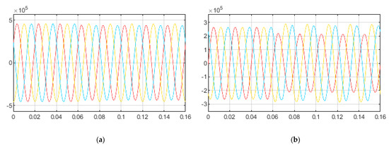
Figure 58.
Scenario No. 4, single-phase fault. (a) Phase-to-phase voltage of M2; (b) Phase-to-ground voltage of M2.
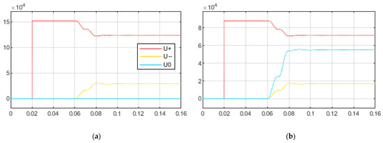
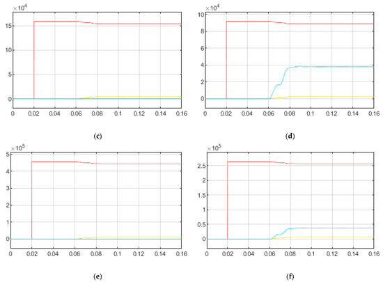
Figure 59.
Scenario No. 4, single-phase fault. (a) Symmetrical magnitudes of the phase-to-phase voltage of M4; (b) Symmetrical magnitudes of the phase-to-ground voltage of M4; (c) symmetrical magnitudes of the phase-to-phase voltage of M3; (d) Symmetrical magnitudes of the phase-to-ground voltage of M3; (e) Symmetrical magnitudes of the phase-to-phase voltage of M2; (f) Symmetrical magnitudes of the phase-to-ground voltage of M2.
3.1.5. Case Studies
Some practical examples will be given in order to support the validity and adequacy of the results in real conditions. Siemens PSS/E software tool is used for calculations. The first example is given in Figure 60: three scenarios are created in the 330 kV grid of the Baltic power system operating in the 2017 mode.
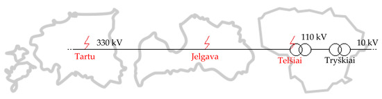
Figure 60.
Simulation scenarios in the transmission grid of the Baltic power system.
The voltage sag matrix is given in Table 14 and it can clearly be seen that the results are not symmetrical. Latvia’s node is the most robust, and Estonia’s node is in second place: if a three-phase fault occurs at Jelgava, then the residual voltage at Tartu is 0.84 p.u., meanwhile at Telšiai it is only 0.31 p.u. If the fault occurs at Telšiai, the residual voltage at Jelgava is 0.63; but otherwise, when the fault occurs at Jelgava, the residual voltage at Telšiai is 0.31 p.u. In both cases, when the fault location is in either Latvia or Estonia, the respective voltage sag is not mitigated at Lithuania’s 110 kV node in Trykšiai; however, when the fault occurs at Lithuania’s node (Telšiai), the residual voltage of Trykšiai is increased by 0.26 p.u. As has been explained before, the result depends on the power-flow direction, the number of power supply lines (or generally speaking on topology) and distances from power plants, also reactive power generated by both reactive power compensation devices and transmission lines, which jointly determine the grid node’s voltage stability, i.e., reactive power–voltage characteristic. Particularly in the case of a three-phase fault, downward propagation does not depend on line length, and upward propagation has a logarithmic nature (see Section 3.1.1).
Table 14.
Three-phase fault voltage sag matrix of the investigated nodes, 2017.
It is noteworthy that Lithuania converted itself from being an electricity exporter to importer after the shutdown of two RBMK-1500 units (Russian: peaктop бoльшoй мoщнocти кaнaльный, PБMK; ‘high-power channel-type reactor’) in Ignalina nuclear power plant (in 2004 and 2009) due to safety concerns. The reactors were initially 1500 MWe (4800 MWt and 1380 MWe net) units, but were later de-rated to 1300 MWe (1185 MWe net) [63]. The construction of the third unit (and plans for the fourth) was suspended (cancelled) after the Chernobyl nuclear accident. In 2007, Lithuania’s parliament adopted a new law on building a new nuclear power plant. The proposed location of the new Visaginas nuclear power plant was (is) next to the existing Ignalina nuclear power plant; however, this project is currently on hold and its prospects remain uncertain. Currently, in Lithuania, both the TSO and DSO are focused on wind and solar parks, and expect to increase installed renewable energy capacity up to 9 GW, which along with other necessary projects will be greatly beneficial for the system including voltage sag mitigation.
The second example—the non-public grid of a chemical plant—is given in Figure 61. The main object of this investigation is the in-plant 6 kV busbar, feeding some technologically important electric motors. Scenario No. 11 occurs at the TSO’s 110 kV switching station, while Scenarios Nos. 12–15 at in-plant nodes: No. 12—the opposite 6 kV winding of three-phase transformer; No. 13—the in-plant point of coupling fed by the opposite winding of a two-winding series reactor; No. 14—the opposite winding of a two-winding series reactor; No. 15—the busbar of direct interest. In this particular case, approximately 50% of outages were caused by faults in the transmission grid, the rest of the reasons were internal. The results—residual voltages (p.u.) at the 6 kV busbar—are also given in the same figure. In Scenarios No. 11 and No. 15, analogously to downstream propagation of Nos. 1–9, a power supply interruption at the motors’ terminals is observed, which also means that an outage is almost inevitable. If a fault occurs at a farther 110 kV node, the consequences will depend on relay protection and automation performance in the 110 kV switching station. In this switching station, similar to the investigation of topological changes of the HV in the test grid (see Section 3.1.1), the following alternatives was disputed: (1) if the circuit-breaker between particular 110 kV busbars is switched on, voltage sags will be felt equally by the both in-plant grid branches; (2) if the circuit-breaker is switched off, the resilience of the in-plant grid is higher (since the 110 kV busbars are more independent), however, the short-circuit ratio is higher too. In the case of upward propagation Scenarios Nos. 12–14, which are similar to No. 3 and No. 5, the residual voltage is higher than 0.40 p.u.; thus, a chance for a successful motor self-starting (and outage avoidance) remains. However, any simultaneous self-starting of the motor group will overload the grid with a high inrush current. Therefore, priority must be given to the most important groups in order to avoid both successive voltage sag and the triggering of overcurrent relays. In this particular case, the highest economic losses can be suffered by interrupting the following processes: both atmospheric and reduced pressure fractional distillations (separation of a mixture into its component parts), hydrodesulfurization (sulfur removal by converting it to hydrogen sulfide H2S, i.e., by adding hydrogen), and catalytic cracking (conversion of high-molecular weight hydrocarbons to lighter products). In spite of that, other critical systems must also be taken into consideration (particularly for safety reasons), for example, fire-fighting systems, the cooling loop, the nitrogen loop [5].

Figure 61.
Simulation scenarios in the industrial grid.
Please note that a three-phase electric motor behaves like a generator upon the occurrence of a three-phase short-circuit (i.e., begins to supply the fault node); thus, the given example is slightly different from the previous cases. The process depends particularly on motor type. For example, the generation of conventional synchronous motors is longer than induction motors; hence, a higher residual voltage (and consequently higher probability of successful self-starting) can be expected [58]. If a motor is equipped with a variable-frequency drive, the drive limits short-circuit current and immediately disconnect the motor; thus, interruption of a manufacturing process can be expected [60].
3.2. Case Study: Faults in the Lithuanian Distribution Grid
3.2.1. Correlation with Grid Reliability Indexes
In 2015–2018, most faults (80% by quantity, 87% by repair duration) occurred in the 0.4 kV grid; however, their influence on total unplanned SAIFI and SAIDI was 15–17%. This can be explained by the low connected customer density, i.e., the fact that the number of customers connected to 0.4 kV nodes is relatively low. Despite a high customer density, the impact of the 35 kV grid on SAIFI and SAIDI was the lowest (up to 5%) due to the following aspects: (1) very low share of the total failure rate (up to 1% by both quantity and repair duration); (2) 35 kV lines have the smallest share of the total length; (3) the 10 kV grid level of automation is sufficient to recover power supply from healthy reserve lines. The share of 10 kV faults was 20% by quantity and 13% by repair duration, but they had the heaviest weight on the reliability indexes—approximately 80%.
The regression analysis of the Lithuanian distribution grid is given in Figure 62, Figure 63, Figure 64, Figure 65, Figure 66, Figure 67 and Figure 68. In all cases, the coefficient of determination (and, respectively, linear correlation) is (very) high, which means a strong interconnection between the annual fault rate and the reliability indexes (correlation with SAIFI is stronger than with SAIDI): almost all correlation coefficients are higher than 0.70 (except the 0.58 of Figure 68b). Please note that events in the 35 kV grid without ACR (Figure 63) are an exception—the relationship does not exist. On the other hand, as has been mentioned before, since the share of the 35 kV grid in total SAIFI and SAIDI was the lowest (up to 5% including ACR events; an average of 32 failures per year excluding ACR events), the appearance of a tendency can be expected with an increase in the number of observations (according to the law of large numbers). Moreover, all values of the tangent of , calculated according to Equation (7), are very small, and a small regression slope means a low sensitivity of change of the function’s output with respect to the input, which is a highly desirable (positive) feature of any electrical grid. Please note that each figure has its own independent (different) scale (adjusted for visualization purposes). It is noteworthy that SAIFI and SAIDI, investigated in this paper, are the most popular reliability indexes. A summary of reliability indexes used by European grid operators can be found in [50] (pp. 34–36).
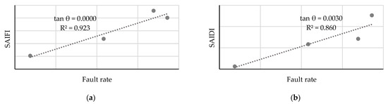
Figure 62.
Regression analysis of the Lithuanian 0.4 kV grid, 2015–2018. (a) Interdependence between SAIFI and the fault rate; (b) Interdependence between SAIDI and the fault rate.
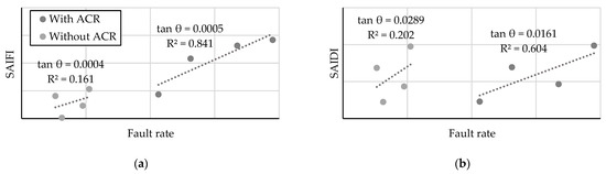
Figure 63.
Regression analysis of the Lithuanian 35 kV grid, 2015–2018. (a) Interdependence between SAIFI and the fault rate; (b) Interdependence between SAIDI and the fault rate.
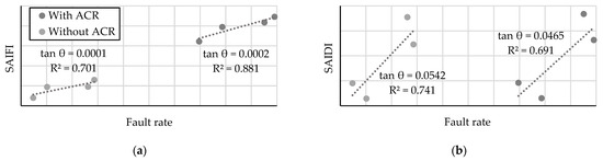
Figure 64.
Regression analysis of the Lithuanian 10 kV grid, 2015–2018. (a) Interdependence between SAIFI and the fault rate; (b) Interdependence between SAIDI and the fault rate.

Figure 65.
Regression analysis of the Lithuanian 10 kV overhead lines, 2015–2018. (a) Interdependence between SAIFI and the fault rate; (b) Interdependence between SAIDI and the fault rate.
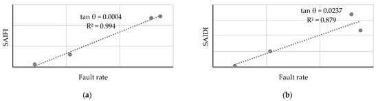
Figure 66.
Regression analysis of the Lithuanian 10 kV cable lines, 2015–2018. (a) Interdependence between SAIFI and the fault rate; (b) Interdependence between SAIDI and the fault rate.

Figure 67.
Regression analysis of the Lithuanian 10/0.4 kV substations, 2015–2018. (a) Interdependence between SAIFI and the fault rate; (b) Interdependence between SAIDI and the fault rate.

Figure 68.
Regression analysis of the Lithuanian 10/0.4 kV transformers, 2014–2018. (a) Interdependence between SAIFI and the fault rate; (b) Interdependence between SAIDI and the fault rate.
Unfortunately, currently, detailed classification by PQ event type is not possible (or is barely possible), thus the term ‘fault’ should be understood in the broader context, i.e., when voltage sag, transient interruption, short interruption, and long interruption are covered. What is more, the type of PQ event observed in different nodes depends on automation and mitigation devices (e.g., distributed generation). Also, it is probable that some part of non-dangerous voltage sags was skipped. As has been mentioned in Section 1, one of the reasons is the absence of massive and fully automated (digitalized) PQ monitoring systems in the world [5]. The second reason is the not clearly (universally) defined boundaries between listed PQ events. A summary of the interruption time thresholds defined by European countries can be found in [50] (p. 24), and some countries do not define all types of interruptions. In Lithuania, the boundary between short and long interruption is 3 min, but the boundary between a transient and short interruption is not set. EN 50160:2010 limits voltage sag duration up to 1 min; however, a 1 min voltage sag whose residual voltage is, for example, 0.1–0.2 p.u. will probably has a similar effect as 1 min interruption (i.e., when the residual voltage is up to 0.05 p.u.). Nevertheless, it is obvious that if operation of ACR is successful, a customer feels a voltage sag/transient interruption or at least short interruption, and it is highly desirable to avoid outage minutes under successful operation of ACR. Since ACR impact has been evaluated with Lithuanian distribution grid data, the situation can be understood through the prism of the methodology of Section 2.3 (Table 15). Firstly, the fewer minutes are lost during ACR events, the higher is the success of ACR (see Equation (4)): the lowest success coefficient (0.9567) belongs to the 35 kV grid in 2016, however, as has been mentioned earlier, the influence of the 35 kV grid on total SAIDI is very low—up to 5% (SAIDI including ACR was 1.4311, excluding ACR it was 1.3691). Secondly, the ACR ratio, defined by Equation (5), is given in the brackets as a supplementary characteristic: the higher the ACR ratio, the lower is its impact on SAIDI, hence the more significant is the success of ACR.
Table 15.
ACR success (and ratio) in the Lithuanian distribution grid.
3.2.2. Probabilistic Analysis of Primary Reasons
Since the hegemony in total SAIFI and SAIDI belongs to the 10 kV grid, greater attention to the primary reasons for its internal faults is paid in Table 16. The following parameters are given: expected annual rate, sample standard deviation, both confidence intervals, and criteria for the evaluation of similarity between the Poisson and Gaussian models (see Section 2.4). All causes are grouped by target group into five categories—overhead power lines, cable lines, outdoor and modular substations, pole mounted substations, and general issues. In approximately 12% of cases, the primary causes were not identified: 7% of them were examined, 5% were not examined.
Table 16.
Statistics of the primary fault causes in the Lithuanian 10 kV grid, 2015–2018.
After an additional aggregation of some kindred groups of Table 16, the following causes can be treated as the most common by quantity (Figure 69): (1) operation of ACR; (2) flora; (3) cable line failure (sample standard deviation unknown); (4) lightning strike or lightning arrester failure; (5) fauna; (6) insulator failure. On the other hand, this does not mean that the rest of the causes are less important—there are many ways of classification, for example, a transformer failure will probably have a more serious economic impact than an unfastened wire, tree branch, or insulator failure.
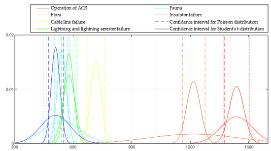
Figure 69.
Probabilistic analysis of the most common primary fault cause frequency in the Lithuanian 10 kV grid. Both Poisson and Gaussian models are given (when confidence level of one-tail is 90%), except cable lines due to unknown sample standard deviation. Please note that all events and their distributions are separate and independent.
Currently, due to limited (absence of) literature on the topic, the exact distributions of each group of Table 16 remain unknown, and an appreciable dissimilarity between the Poisson and Gaussian models can be noticed in Figure 69 (except the lightning events group). Also, it should be kept in mind that PQ event distributions are (can be) dependent on PQ mitigation (along with preventive) measures (projects). On the other hand, according to the central limit theorem, in many cases a sampling distribution of independent and identically distributed random variables tends towards the normal distribution with an increase in the number of observations. Let us take a deeper look into the Gaussian and Poisson models similarity when the continuity correction error is smaller than 2.5%, which is reached when is 100 or greater (see Table 16): both boundary cases, determined by the sum of and (see Equation (27)), are given in Figure 70. In Figure 70a, a large dissimilarity is seen between the Gaussian and Poisson models. Conversely, in Figure 70b, the Gaussian model is almost identical to the Poisson model.
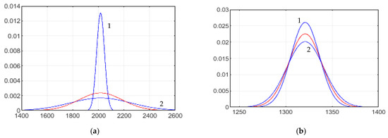
Figure 70.
Convolutions of the Poisson and Gaussian models. (a) Case of shrub grow-in (overhead power lines); (b) Case of humidity, rain, snow, and dust (outdoor and modular substations). Legend: 1 (blue curve)—autoconvolution function of the Poisson distribution; 2 (blue curve)—autoconvolution function of the Gaussian distribution; red curve—convolution function.
Finally, let us discuss confidence intervals. Two significance levels are used in Table 16. In our opinion, the 0.10 level is a more suitable significance level for the Lithuanian distribution grid (due to errors and uncertainties during the collection and classification of data), however, 0.05 is the most widely used. When the significance level is lower, the confidence interval is broader. It can be noticed that the confidence interval of the Poisson distribution is asymmetrical: for discrete distributions, it is often difficult (impossible) to obtain the interval with an exact confidence level , due to the discrete nature of the statistics [62]. Misinterpretation of confidence intervals and levels is a common problem even among highly qualified scientists. This topic has been studied by [64,65]. The confidence level is connected with the reliability of the estimation procedure: once the interval is calculated, it either covers the value of a (respective) population parameter or not; thus, the confidence level is not a probability of this coverage.
3.2.3. Case Studies of Two-Dimensional Probabilistic Analysis
In anticipation of Smart Grids and the interoperability of their applications, the investigation of many events should be comprehensive (multidimensional). Two-dimensional probabilistic analysis is based on the conditional probability definition given by Equation (28). Obviously, such an investigation is possible only when information about the probability distribution of the second event is available. Let us begin with lightning events (Figure 71), which are among the six most common groups in the 10 kV grid (see Figure 69). The available division of the territory of Lithuania into lightning zones regarding annual thunderstorm duration can be found in [5,66]. This kind of analysis is beneficial for the field of lightning security (including the shielding of both substations and buildings), lightning arrester placement strategies, calculations of induced voltage in overhead power lines (including exceeding safe touch voltage). The cumulative distribution function of negative first stroke current can be found in [67]: a crest current up to 200 kA is expected. Usually, the first stroke is followed by 2–10 successive strokes with 0.03–0.05 s intervals between them [66]. When the cumulative distribution function is known, the probability density function is obtained as follows:
where: —the crest current of the stroke, kA.
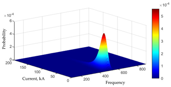
Figure 71.
Probabilistic surface of the Lithuanian 10 kV grid faults caused by lightning.
Next, the analysis through a prism of repair duration is beneficial for outage management (including the economic consequences assessment), network modes planning, operational switching. The parameters of repair hour distribution can be determined from information given in [56]: currently, it should not be critical that power transformer repair data is from 1995–2000, but an update is desirable. The probabilistic surface, shown in Figure 72, depicts the average situation in the case of the voltage of the transformer’s primary winding is either 110 kV or 35 kV: the Gaussian distribution is combined with the gamma distribution (shape parameter is 0.12 and scale parameter is 18.4). In 1995–2000, the most common fault types, determined by transformer oil testing, thermography, insulator testing, vibro-acoustic testing, and other methods, were the following: commutator or tap changer failure (24%), fan or pump failure (19%), partial discharge (16%) [56].

Figure 72.
Probabilistic surface of transformers, whose voltage of primary winding is either 110 kV or 35 kV, faults and their repair duration.
The last and the most widely understood example is the failure rate dependence on exploitation age. In general terms, the failure rate of a device can be represented with a bathtub curve [55,56]. This U-shaped curve has three regions: (1) decreasing rate due to early failures (in particular manufacturing defects); (2) constant rate due to random failures; (3) increasing rate due to the ageing process. Despite being well-known, the curve does not have a universally agreed mathematical expression. Moreover, it is also not known whether a particular device will follow it (especially under proper maintenance). According to [56], the Weibull distribution, whose shape parameter is 0.5 and scale parameter (determined from given constants) is approximately equal to 280, must be used for 10-year period failure rate evaluation of power transformers (whose primary winding voltage is either 110 kV or 35 kV). However, as can be seen in Figure 73a, this model represents only the first region of the U-shaped curve. There are models which can cover all three regions—for example, the beta distribution in the case of both shape parameters and is (approximately) equal, positive, and smaller than 1 (Figure 73b). However, some questions can be raised about beta model flexibility. To sum up, the following approaches can be used:
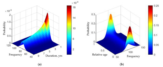
Figure 73.
(a) Probabilistic surface of power transformers, whose primary winding voltage is either 110 kV or 35 kV, faults through a prism of exploitation age for the first 10 years; (b) Probabilistic surface of sleeves faults through the prism of exploitation age.
- 1.
- When a U-shaped curve is modeled using a single function, for example, beta distribution (as in Figure 73b);
- 2.
- When all three regions of a U-shaped curve are mutually exclusive, thus a sample space is formed as follows:
- 3.
- When the second zone of a U-shaped curve is interpreted as mutually inclusive event, then addition rule formula gives the following expression:
4. Discussion
4.1. PQ Monitor Allocation through the Prism of a Voltage Sags Propagation Mechanism
As has been mentioned in Section 1, the development of efficient and cost-effective PQ monitoring systems is inhibited by a lack of literature on the topic of the voltage sags propagation mechanism. Currently, only two lemmas regarding voltage and current monitoring are known (see Section 1). Since these lemmas are derived from Ohm’s law, their application requires an input of grid impedances, which indicates low practical significance [5]. Therefore, let us summarize the results of Section 3.1, and derive the new rules (principles) which would be easier to apply in practice for PQ monitor displacement in order to optimize monitoring of both symmetrical and asymmetrical faults. This is a method of inductive reasoning—when a general principle is derived by making a generalization based on a specific observation (Figure 74a). Since inductive reasoning is based on empirical research, the correctness of a conclusion is probable but without absolute certainty (and additional evidence may be required). The method depends on the quality of observation. The opposite is the deductive reasoning method (Figure 74b): since it is based on logic, a deduction’s conclusions are always bulletproof as long as the premises are true (and assuming that mistakes in the logic chain are avoided). However, deductive reasoning cannot be applied in the case of PQ data, because PQ is a newly emerging (scientific) field [5], hence the theory is not formed.
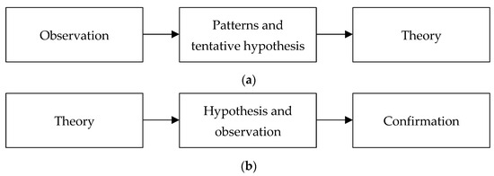
Figure 74.
(a) Inductive reasoning method; (b) Deductive reasoning method.
Due to it having the highest level of penetration, the three-phase short-circuit is the simplest case to monitor. Moreover, it is the simplest case to analyze due to its symmetry. “Which voltage should be measured (assessed)?”—is a common PQ question arising from both technical and juridical sides. Both voltages are not often monitored simultaneously: for example, see the questions and results of the international survey on PQ monitoring in [68]. Therefore, for the symmetrical case, the following axiom must be established:
Axiom 3.
In the case of a three-phase fault, both phase-to-phase and phase-to-ground voltage sag depths are equal and independent of neutral mode.
It is obvious but must be explained that this axiom and all other principles in this subchapter are correct when the essence is not artificially altered, especially with PQ mitigation devices. For example, a single-phase generator is able to distort the original patterns of a three-phase fault. Moreover, it is realistically assumed that the spark of a short-circuit does not damage the transformer and does not physically pass to its other winding(s). Also, the phrase ‘at transformer’s winding’ defines not only the winding but also its near vicinity—let us say up to 100–200 m, but the estimation of a more precise threshold could be a further research avenue. These assumptions (conditions) are fully reasonable and correct, because the main focus is made on voltage sag behavior, but not on the efficiency of PQ mitigation devices. In addition, the condition of an absence of voltage unbalance before fault must be met. When these conditions are fulfilled, other conclusions, derived from Section 3.1.1, are as follows:
- Three-phase voltage sag propagation strongly correlates with power-flow direction:
Lemma 4.
If the directions of power-flows are known (particularly after the fault), then the downstream propagation path of a three-phase voltage sag is known.
- 2.
- Upward voltage sag propagation dependence on the 330 kV line length in the case of Scenario No. 2 is investigated in Figure 9. However, since the model of generator (swing voltage source) has been selected according to the traditional approach of power-flow studies, it would be desirable but difficult to support this research with practical experiments encompassing various types of generators. Also, it has been found that if a transmission grid fault (Scenarios No. 2 and No. 4) does not propagate upwards, then an occurrence of a voltage transient is highly expected at least in HV lines. The transient can be observed not only in busbars which directly supply the fault node, but also in more distant segments such as the right branch of this paper’s test scheme. It would also be beneficial but difficult to support this finding with practical experiments. Moreover, it has been noticed that the same principle is also characteristic to all types of asymmetrical faults. Therefore, considering the above, the following principle, regarding voltage sag propagation upwards, is established for the transmission grid:
Principle 5.
A sudden occurrence of a high-voltage transient is characteristic of upward propagation of a three-phase fault; and thus, can indicate a nearby fault in either the same or lower level of a high voltage grid.
- 3.
- In the case of a downstream propagation from Scenarios Nos. 1–7, the following generalization is established:
Lemma 6.
If power flows from transformer winding No. 1 to winding No. 2 (and No. 3), and a three-phase voltage sag propagates downstream (from winding No. 1), then the same voltage sag depth is observed at all windings.
- 4.
- After the investigation, it has been found that Lemma 6 cannot be applied vice versa (see Scenarios Nos. 5–9). Thus, the additional definition is required:
Lemma 7.
If power flows from transformer winding No. 1 to winding No. 2 (and No. 3), and a three-phase voltage sag is observed at winding No. 2 (or No. 3), then voltage sag depths at the rest of the windings remain unknown.
- 5.
- Firstly, in the case of the only investigated 330/110 kV autotransformer, when a three-phase fault occurs at the tertiary winding (Scenario No. 3), the voltage sag depth at the common winding is 90% (see Table 1). Conversely, when the distance from the tertiary winding (along the same 10 kV line) is increased by at least 0.5 km (modification of Scenario No. 3), no sag is observed at the tertiary windings (see Figure 13). Secondly, after the deeper investigation of the 110/35/10 kV three-winding transformer (M4, M5 and M5c) in the case of Scenarios No. 5 and No. 6, and considering the maximum possible length of MV lines, Lemma 7 is supplemented with the following principle:
Principle 8.
If power flows from HV/MV/MV transformer winding No. 1 to windings No. 2 and No. 3, a three-phase fault at any point of MV line, directly fed by winding No. 2 (No. 3), propagates upwards to winding No. 3 (No. 2), but does not propagate to winding No. 1.
Let us continue with asymmetrical faults. More aspects come out in the case of the monitoring and assessment of these faults, due to a shorter propagation path, different but hardly distinguishable patterns (since they depend on many factors) and their rotation (see Table 4, Table 5, Table 6, Table 7, Table 8, Table 9, Table 10, Table 11, Table 12 and Table 13). Moreover, PQ observation is limited by technical possibilities, and one of the reasons is that existing voltage transformers were originally designed for energy accounting purposes. For example, most (older) voltage transformers in the Lithuanian MV grid are grounded and measure phase-to-ground voltage, but EN 50160:2010 requires assessment of phase-to-phase voltage of three-wire systems. Next, most older 10 kV voltage transformers do not have a transformer in one of three phases. This phase is grounded in the case of either configuration (star or delta). However, during an asymmetrical fault, Axiom 3 does not apply but the PQ analyzer assumes that the mode is symmetrical, thus the correctness of the voltage estimation procedure cannot be expected. Such an example of an asymmetrical fault is given in Figure 75 (from the results of the PQ measurement campaign in the Lithuanian DSO grid). A sudden increase in two measured currents, followed by the disconnection of the line, is seen in Figure 75a. Since the short-circuit is asymmetrical, estimation of phase-to-phase voltages, given in Figure 75b, is incorrect.
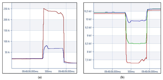
Figure 75.
Asymmetrical fault in the Lithuanian 10 kV grid. (a) Available measurements of current; (b) Estimated phase-to-phase voltage: since only two voltages were measured and Axiom 3 does not apply, the estimation of voltage is incorrect.
Let us begin with the two-phase-to-ground short-circuit. The following conclusions are derived from Section 3.1.2:
- Principle 5 applies.
- Similarly (but not analogously) to Principle 5, the interconnection with voltage unbalance has been found in the case of upstream propagation of an MV grid fault (Scenarios Nos. 5–7). The difference in upstream propagation is that the unbalance weakens, while the transient does not. Since voltage unbalance is usually caused by loads, the application of this relationship can be expected only after full interoperability between PQ and others Smart Grid’s applications which measure the consumption and the unbalance—in particular, meter data management (or an advanced metering infrastructure) and substation relay protection and automation. In the case of Scenario No. 6, this principle is explained in Figure 32, and is also characteristic of a two-phase fault. In general, this unbalance (to be exact, only the negative sequence) should be higher than 2% (e.g., in Scenario No. 6, the negative sequence unbalance of both phase-to-ground and phase-to-phase voltages of M4 is 2.3%); however, more in-depth research on the topic is required. Currently, this principle is established as follows:
Principle 9.
If power flows from either an HV/MV or MV/MV transformer winding No. 1 to winding No. 2 (and No. 3), a sudden occurrence of voltage unbalance at winding No. 1 is characteristic of upward propagation of both two-phase-to-ground and two-phase faults; and thus, can indicate the fault at any point of the MV line connected to winding No. 2 (or No. 3).
- 3.
- In the case of Scenario No. 4, when a two-phase-to-ground fault occurs in the HV grid, the voltage unbalance is observed at all windings of the 330/110 kV autotransformer (see Table 6 and Figure 31). The distance between the fault node and the autotransformer is 55 km. Since the HV grid’s lines are considerably longer, more in-depth research is needed in order to establish a generalization for upward propagation of two-phase-to-ground faults in an HV grid (similar to the previous case), including separate examination of differences between a transformer and autotransformer.
- 4.
- In the downstream propagation path, rotation is often (but not always) observed in interruption, sag, swell, and RVC events. This rotation is not random (chaotic), which means there is a possibility of feature extraction. The example of voltage pattern dependence on winding configuration is given in Figure 32. However, more in-depth research on the topic is required in anticipation of AI algorithms.
- 5.
- In the case of downstream propagation, Lemma 4 applies partially, due to observed conversions from interruption to sag (e.g., the phase-to-ground voltage of both phase A and phase B in Scenarios No. 6 and No. 7).
- 6.
- More observations are needed for a generalization of phase-to-ground voltage swell behavior caused by a two-phase-to-ground fault in an HV grid. Meanwhile, in the case of an MV grid (Scenarios Nos. 5–7), it is seen that voltage swells do not propagate through transformers in both directions. Moreover, in the case of an LV grid (Scenarios No. 8 and No. 9), voltage swells do not propagate upwards through the 10/0.4 kV transformer. These principles are also characteristic to a single-phase fault (see Table 12). Therefore, based on our experience gained during the PQ monitoring campaign in the Lithuanian DSO grid, and considering the above, the following axioms are established:
Axiom 10.
Phase-to-ground voltage swell, caused either by a two-phase-to-ground or single-phase fault in an MV grid, which operates in isolated (compensated) neutral mode, does not propagate through a transformer in both directions—upstream and downstream.
Axiom 11.
Phase-to-ground voltage swell, caused either by a two-phase-to-ground or single-phase fault in an LV grid, which operates in grounded neutral mode, does not propagate upstream through an MV/LV transformer.
- 7.
- Currently, from the juridical point of view, it is not clear (agreed) which assessment method of fault node incurs lighter/heavier legal liability, i.e., which voltage sag depth array is better: (1) one phase-to-phase voltage interruption with two 10–50% depth sags, or (2) two phase-to-ground voltage interruptions with one swell (see Table 7). In our opinion, the phase-to-phase assessment method is lighter.
Let us continue with the two-phase short-circuit; the following statements are derived from Section 3.1.3:
- Principle 5 applies.
- Principle 9 applies.
- In the case of downstream propagation, Lemma 4 applies partially, due to observed conversions from interruption to sag (similar to the previous case).
- Voltage swell is not characteristic; thus, analysis of the downstream propagation path should be simpler than in the case of two-phase-to-ground fault. Additionally, according to Table 10, fault node patterns almost do not depend on fault location; however, more observations would be beneficial before generalization.
- Currently, from the juridical point of view, it is not clear (agreed) which assessment method of fault node incurs lighter/heavier legal liability, i.e., which voltage sag depth array is better: (1) one phase-to-phase voltage interruption with two 10–20% depth sags, or (2) one healthy phase-to-ground voltage with two 40–50% depth sags (see Table 10).
Lastly, in the case of single-phase short-circuit, the following statements are derived from Section 3.1.4:
- Principle 5 applies.
- Principle 9 does not apply.
- Lemma 4 does not apply. Axioms 10 and 11 apply (for MV and LV grids). More observations of single-phase fault behavior are needed for generalization in both cases: (1) when the fault occurs in an HV grid (Scenarios No. 1, No. 2, and No. 4), and (2) when the fault occurs at the three-winding transformer’s secondary (or tertiary) winding (Scenario No. 5). If the single-phase fault occurs at the autotransformer’s tertiary winding (Scenario No. 3), it does not propagate to the HV grid. Considering the above, the following axioms are established for both MV and LV grids (Scenarios Nos. 6–9):
Axiom 12.
If a single-phase fault occurs in an MV grid, which operates in isolated (compensated) neutral mode, and not at either the secondary or tertiary winding of a three-phase transformer, then it does not propagate through this transformer in both directions—upstream and downstream.
Axiom 13.
If a single-phase fault occurs in an LV grid, which operates in grounded neutral mode, and not at either the secondary or tertiary winding of a three-phase transformer, then it does not propagate upstream through the MV/LV transformer.
- 4.
- Single-phase faults do not affect phase-to-phase voltage of both MV and LV grids, except a slight impact om M5 and M5c in Scenario No. 5, when the fault occurs at the tertiary winding of the three-winding transformer. Therefore, when the situation in a three-wire system is assessed according to EN 50160:2010, grid operators will avoid responsibility. Despite this, it will be important to monitor phase-to-ground voltage, for example, in order to evaluate the negative impact on insulation caused by voltage swells. Conversely, if a single-phase fault occurs in an HV grid, the impact on phase-to-phase voltage is clearly seen. Considering the above, the following axiom is established:
Axiom 14.
If a single-phase fault occurs in either an MV or LV grid, which, respectively, operate in isolated (compensated) and grounded neutral modes, and not at either the secondary or tertiary winding of a three-phase transformer, then phase-to-phase voltage is not distorted.
- 5.
- Upward single-phase voltage sag propagation dependence on the 330 kV line length in the case of Scenario No. 2 is investigated in Figure 10 (see Section 3.1.1). Analogously to Figure 9, it would be beneficial but difficult to support this research with practical experiment encompassing various types of generators.
- 6.
- From the juridical point of view, as has been mentioned previously, it is obvious that if Axiom 14 applies (for both MV and LV grids), the phase-to-phase voltage assessment method allows grid operators to avoid legal liability. Conversely, in the case of an HV grid, it is not clear (agreed) which assessment method of fault node is lighter/heavier (see Table 13), but in our opinion, it seems to be obvious that the phase-to-phase assessment method is lighter.
The full development of voltage sags propagation theory will advance monitoring solutions and allocation strategies to the next level. The choice of PQ monitor allocation strategy depends on the desired aim [5]. Based on Axioms 12 and 13, it can be concluded that the goal to monitor single-phase faults will require the most resources: since voltage swells are harmful for insulation, this event cannot be ignored in anticipation of the application of predictive maintenance. One of the cost-saving options is usage of limited functionality monitors, for example, PQ-measuring smart meters (see [5] for application details in Lithuania) and protective relays (e.g., negative sequence relays based on Principle 9). Despite this, the study answering many questions and laying a theoretical foundation for the voltage sags propagation mechanism, many aspects still remain unanalyzed. For example, the propagation mechanism in ring topology, and pattern dependence on winding configuration have been only slightly analyzed in this paper. Moreover, along with [5], the idea about interconnection among PQ events has been raised for the first time, slightly investigating the cases of voltage sag relationships with interruption, RVC, swell, transient (also see the first part of Section 4.3), and unbalance. It is noteworthy that there is other obvious relationship between voltage sag (as well as the caused transient), harmonics and inter-harmonics: even if the sag is avoided due to perfect operation of the grid’s automation, commutation processes will cause short-time harmonics and inter-harmonics. Another further research avenue can be related to voltage sags caused by an electric motor starting, including focus on self-starting and motor groups—some details on the topic are given in the end of Section 3.1.5. The third research avenue is the incorporation of PQ mitigation devices (see Section 4.2.2), also specific grids—for example, a traction power network (for railways, trams, and trolleybuses), and HVDC lines. Moreover, it would be beneficial to support the results with practical measurements. However, any artificial creation of voltage sags in real systems is impossible; for that reason, statistical and probabilistic analyses (such as in Section 3.2) gain in importance.
4.2. PQ Monitor Allocation through the Prism of Grid Reliability
PQ monitoring is important not only for compliance verification or physics investigation, but also for power system development, its investment planning, and its economic analysis (in particular, cost savings due to the diminished number of events and avoided outages). Let us explain the Lithuanian DSO’s investment planning scheme by defining the distribution grid segment as a radial branch (consisting of both MV and LV levels) connected to its HV/MV transformer. It is noteworthy that another approach to the term could be based on the administrative division. The segment is selected for monitoring if its SAIFI and SAIDI are higher than the values in the DSO’s 10-year investment plan. If planned investments can enable the achievement of these values within 3 years, monitors are not installed. The projects can be divided into primary and secondary. Primary projects are the prevention of undesirable dangerous events (see Table 16). Secondary projects are focused on the installation of PQ mitigation devices. Discussion on the topic is continued in Section 4.2.1 and Section 4.2.2.
4.2.1. Flora and Fauna
As has been determined in Section 3.2.2, flora and fauna are among the five most common primary fault causes by quantity (see Figure 69), and flora is even in second place after ACR events. Meanwhile in Minnesota [57], flora is in third place and fauna in seventh by influence on both SAIFI and SAIDI. However, the result depends not only on geography, grid maintenance, and PQ mitigating devices but also on classification. In Minnesota, first place belongs to the weather (27% SAIFI, 72% SAIDI); however, this group is not formed for overhead power lines in Table 16, because weather (in particular wind) is mutually related with flora. Typical examples of flora interference in overhead power lines are shown in Figure 76. Despite 0.4 kV lines being shown, the examples are also suitable for the cases of both 6 kV and 10 kV, due to similar (identical) poles (including by height).
Figure 76.
Typical examples of fauna interference with the public grid in Lithuania. (a) A shrub beneath a 0.4 kV line; (b) A 0.4 kV line in the forested area.
A shrub growing beneath a double-circuit three-phase 0.4 kV line is shown in Figure 76a. Many species of tall and fast-growing shrubs (small trees) are native to Lithuania: for example, the typical height of great sallow (Salix caprea) is 2–13 m, the typical height of bird cherry (Prunus padus) is 3–12 m (sometimes up to 16 m). The importance of each situation depends on end-user criticality and specifics: for example, garden or garage community lightning with sodium-vapor lamps probably is not a priority case. One of necessary preventive measures is vegetation management: in 2019, after vegetation clearance, no failures were recorded in 87.3% of the DSO’s overhead lines during the following year (the situation was improved by 22%).
The risk of falling branches is obvious in the case of the tree tunnel in Figure 76b. On the other hand, these tunnels can be characterized by lower risk of bird impact, in particular large birds such as golden eagle (Aquila chrysaetos), whooper swan (Cygnus cygnus), mute swan (Cygnus olor), or white stork (Ciconia ciconia) which breed in open farmlands, in people’s neighborhoods, or near marshy wetlands. The wingspan of the golden eagle is up to 230 cm, the whooper swan—up to 245, the mute swan—up to 240, the white stork—up to 215. According to some unofficial data in [69] (p. 7), published by the Lithuanian Ornithological Society, in Lithuania, approximately half of all storks build their nests on electricity poles. According to the “LIFE Birds on Electrogrid” final report [70], in Lithuania, 45 thousand bird deaths caused by collisions with the TSO grid are expected annually, and the mortality can be reduced by 1.2–4 times with visibility-increasing measures. For example, during the project period, 112 dead mute swans were found in the Nemunas river, in Kaunas; and photos of both golden eagle and whooper swan killed by collision with the wires can be found in [71]. Please note that the collision by itself does not cause electrical problems—two wires (or points with different electric potential) must be touched simultaneously to cause a short-circuit. There is no research regarding correlation (proportion) between the number of bird collisions and voltage sags/interruptions, but it is reasonable to expect that a reduction of bird mortality will improve PQ. It can be implemented by installing bird collision mitigation measures, also by consideration of migration routes at the power system planning stage.
4.2.2. PQ Mitigation Techniques
Firstly, as has been mentioned before, one of the most obvious preventive measures is the increase in the percentage of underground cable lines. European country data for 2018 can be found in [50] (p. 80): for example, in Lithuania, the share in the LV grid was 32.4%, and in the MV grid—27.3%. Underground cables do not have visual impact, which is desirable in urban environments. However, it is clear a priori that both repair and fault location search processes are significantly more complex in comparison with overhead power lines. Secondly, an efficient PQ mitigation system is one of the ultimate aspirations of all PQ research (in particular this paper). However, despite many papers, a lot of questions remain about PQ mitigation devices, their application (allocation strategy), classification, etc. For example, [13] uses a classification into single power supply and dual power supply equipment, and investigates features of the following devices: dynamic voltage restorer—DVR, solid-state transfer switch—SSTS, static synchronous compensator—STATCOM, static VAR compensator—SVC, unified PQ conditioner—UPQC, and uninterruptible power supply—UPS. Each device has its own unique features; thus, the mitigation efficiency will also be selective and depend on voltage sag parameters (e.g., voltage level, duration, energy, rise time) [5]: for example, STATCOM (with IGBTs) has a shorter response time than SVC (with thyristors).
Let us introduce an example of PQ mitigation research (Figure 77), performed with Siemens PSS/E software tool. Voltage sag mitigation of capacitor banks is compared with a flywheel system under the following situation: (1) the device is installed on the 10 kV line of a 10/0.4 kV substation, which feeds a manufacturing plant of polymer film packages; (2) the investigated node is the other end of the same 10 kV line in the 110/10 kV substation; (3) a three-phase fault occurs at the selected farther node of the 110 kV grid. The fault duration is 0.15 s. Voltage sag/interruption avoidance is a critical issue for this industrial plant, because an outage will not only deteriorate the quality of the plastic, but also will lead to the production line’s equipment clogging. Please note that a short-circuit at another 110 kV node will cause a different (depth) voltage sag, but the nature of the mitigation process will be similar.
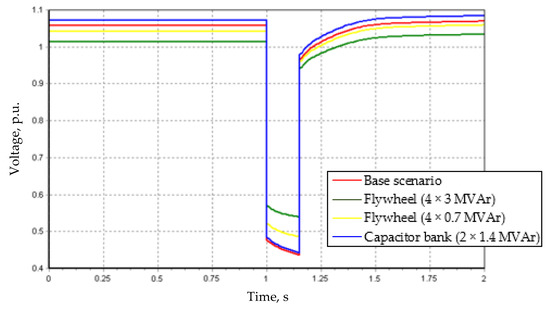
Figure 77.
Voltage sag mitigation efficiency comparison of capacitor bank and flywheel systems on the 10 kV side of a 110/10 kV substation, when the PQ mitigation device is installed on the same 10 kV line at the 10/0.4 kV substation. The voltage sag is caused by a three-phase short-circuit which occurs at the selected farther node of the 110 kV grid.
In Figure 77, it is seen that the investigated flywheel system mitigates the voltage sag by up to 0.1 p.u. (from 0.45 p.u. up to 0.55 p.u.). Even such a small mitigation has some importance and increases interruption avoidance probability; however, currently, this remains a direction for further research. Meanwhile, the capacitor bank is not efficient due to the following reasons: (1) a relatively long response time required for the activation of all levels (to achieve the highest possible capacitance); (2) the power of capacitor is proportional to the voltage square:
where: —capacitance, F; —voltage, V.
4.3. Mathematical Tools—A Further Research Avenue
In the field of PQ, the application of many AI algorithms (e.g., Fourier transform, Kalman filter, wavelet transform, S-transform, Hilbert–Huang transform, Gabor transform, etc.) were reviewed by [72], and this still remains an open field of research. However, since [72] focuses on PQ disturbance classification and feature extraction, it does not cover two important aspects of analysis of voltage sag behavior: (1) strong interconnection between PQ events (the idea has been raised for the first time in [5]); (2) the method of the voltage sag matrix. Some cases of voltage unbalance, caused by a voltage sag, were investigated in Section 3; thus, let us now have a closer look into transients caused by voltage sags, through the prism of wavelet transform. It is a recent but promising tool in many fields, such as audio or video signal processing for noise suppression, also in biomedical signal processing (e.g., electrocardiogram analysis). According to the general and well-known definition, the relationship of the mother wavelet to the daughter wavelet is the following:
where: —scaling factor (positive real); —shift factor.
Wavelet transform is based on wavelet function convolution with input signal as follows:
where: —the complex conjugate of the mother wavelet.
Let us introduce an investigation example with one of the most famous Haar wavelet family. Haar wavelet’s mother wavelet function is as follows:
The transient of phase C (cyan curve) of Figure 7b (Scenario No. 2, three-phase fault, phase-to-ground voltage of M1) is selected for the investigation. The region of direct interest is 0.04–0.10 s because the transient begins at 0.06 s: the array consists of 60,000 samples (sampling time is 10−6 s), and, respectively, the element number, corresponding to the moment the event begins, is 20,000. At the first level of discrete wavelet transform, the transient signal is simultaneously passed through low-pass and high-pass filters, and both arrays are decimated by 2. Output from the high-pass filter gives the detail coefficients, while output from the low-pass filter—approximation coefficients. At the next level, the initial signal is replaced by the approximation signal, and the procedure is repeated. The process is usually represented with a wavelet decomposition tree. The details coefficients by decomposition level are given in Figure 78. Since the 50 Hz component has not been removed, levels 8–12 should be analyzed critically, because the involvement of a 50 Hz signal is visible even before the transient, i.e., during 0.04–0.06 s. At the initial period of the transient, some high coefficients can be observed at the lower levels. The differences between levels (determined by the scaling factors) are clearly seen in Figure 79, where the signal details are given in superimposed mode.
Figure 78.
Detail coefficients of multilevel decomposition.
Figure 79.
Signal details displayed in superimposed mode, where darker colors correspond to the higher levels.
The next important avenue for further research is the development (extension) of the voltage sag matrix method. In this paper, the analysis of voltage sag matrixes is not very complex due to the following reasons: (1) all test schemes are incomparably smaller than real systems; (2) mainly radial topology has been investigated with the specially adapted numeration for the simplicity of analysis. However, all voltage sag matrixes, which are constructed according to current concept (including this paper), will be hard to understand through a topological prism, especially in the case of large power systems (in particular, ring topology) even with the best possible numeration. Therefore, let us introduce the improvement of the method on a typical BRELL transmission grid by designing schemes given in classical literature [59], and begin with the simplest three-phase fault case. The chosen schemes and their voltage sag vector in the case of a three-phase short-circuit occurring at node No. 4 are given in Figure 80. But the overall situation becomes much more understandable with the construction (proposal) of these vectors’ topological extensions (which are also shown in the same figure): for example, in the case of Figure 80a, it is clear that fault location (node No. 4) is fed by nodes No. 1, No. 3, No. 5, and No. 7, and in the case of Figure 80b—by No. 1, No. 3, and No. 5. The centers of loops are depicted (represented) with inner gray cells.
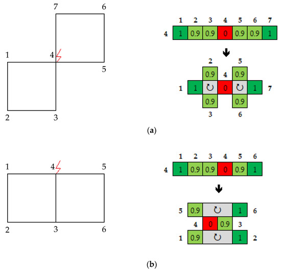
Figure 80.
Examples of a voltage sag matrix topological extension, when a three-phase fault occurs at node No. 4. (a) A case when two rings are connected with a mutual node; (b) A case when two rings are connected with a mutual line.
Let us continue the investigation of the proposed topological extension, and introduce a new analysis concept based on field theory. As has been concluded before, since voltage sags propagation strongly correlates with power-flow direction, the situation can be modeled as an elementary vector field, where the flux can be pointed either to a node or from a node. In normal operation mode, the divergence of each ordinary node will be equal to zero (according to Kirchhoff’s current law), the divergence of generation nodes will be greater than zero (source of the field), and the divergence of end-user nodes will be lower than zero (sink of the field). In the case of a short-circuit, the divergence of the fault node will become lower than zero due to the flux leakage to the ground. According to the general definition, the divergence of a vector field at a point is defined as a limit of the closed surface integral when the volume of this surface shrinks to zero. Considering this, the definition for a cell (grid node) of a voltage sag matrix is derived as follows:
where —the continuously differentiable vector field composed of , , and ; —volume with boundary ; —the scalar product of and the infinitesimal element of vector area (defined as the unit normal scaled by the area, i.e., ); —the vector field of the apparent power-flow composed of ; —the apparent power-flow flowing to ; —the apparent power-flow flowing from .
Another field operator—curl (also known as a rotor)—could also be useful as a supplementary parameter in the gray cells of the topological extension (see Figure 80). It can show whether the electric current flow forms a closed loop (circulation), which can also be important for the prediction of voltage sag behavior. It is obvious that the existence of circulation in all rings is limited by Kirchhoff’s current law, hence it is possible only in some—probably, in the most important (critical) rings. Thus, in normal operation mode, the current can either form a closed loop (either clockwise or counterclockwise) or not—which means a total of three different conditions. Conversely, in emergency mode, the loop cannot be formed; therefore, sudden disbanding of the circulations without operator intervention (e.g., remote control of a circuit-breaker) can indicate the fault. It is noteworthy that this method does not require any PQ analyzers. According to the general definition, the rotor of a vector field at a point is defined by the closed line integral along boundary when the enclosed area shrinks to zero. Considering this, the definition for a center cell of a contour in a voltage sag matrix topological extension is derived as follows:
where: —the continuously differentiable vector field composed of , and ; = the area with boundary ; —the scalar product of and infinitesimal element pointed in the direction of the contour tangent line at ; , and —the unit vectors; —the center cell with indexes ; —the apparent power-flow vector of contour . Thus, according to this equation, circulation exists and the rotor is equal to (corresponds to clockwise or counterclockwise), if vector sum of in two-dimensional space is equal to zero.
5. Conclusions
- 1.
- During the PQ monitoring campaign in the Lithuanian distribution grid, development of a PQ monitor allocation strategy was inhibited by a lack of literature about voltage sags propagation mechanisms: only Lemmas 1 and 2 were known at that time, but their application in practice is challengingly hard (see Section 1). Simulation with the created BRELL-based test grid resulted in the generalization of a voltage sags propagation mechanism by establishing Axioms 3 and 10–14, Lemmas 4, 6, and 7, and Principles 5, 8, and 9 (see Section 4.1). This paper is the first, which not only investigates voltage sags propagation in detail, but also does it in a complex way by considering both voltages, all short-circuit types, interconnection with transient (Principle 5) and unbalance (Principle 9), etc. The method, based on a voltage sag matrix (which has so far been used only for symmetrical faults) has been expanded and adjusted for asymmetrical faults. In addition, the matrix’s topological extension along with established definitions in Equations (39) and (40) has been proposed as a further research avenue (see Section 4.3).
- 2.
- Regression analysis of the Lithuanian distribution grid showed that almost all correlation coefficients between the number of events and the reliability indexes (SAIFI and SAIDI) are higher than 0.70 (see Section 3.2.1). The values of the tangent of , calculated by Equation (7), are lower than 0.08, which means a low sensitivity (see Equation (8)). This paper is the first which proposes the highlighting of ACR events by a new method for the evaluation of ACR success and ratio (Equations (4) and (5)). All values of ACR success are higher than 0.956, which corresponds with a favorable situation.
- 3.
- The 10 kV faults (20% by quantity, 13% by repair duration) had the highest impact on total SAIFI and SAIDI (approximately 80%). The most common events in the 10 kV grid by quantity were ACR, flora, cable line failure, lightning, fauna, and insulator failure (see Section 3.2.2). Since the distributions of all the events listed in Table 16 are not known, probabilistic analysis has been performed by using two models—the Gaussian and Poisson. For estimation of their similarity, when the continuity correction error is calculated using Equations (21) and (22), a new and universal approach is proposed—criteria and are defined by Equations (25) and (26) (see Section 2.4).
Author Contributions
Conceptualization, V.L. and V.R.; methodology, V.L., V.R. and G.K.; software, V.L., V.R., G.K. and D.N.; validation, V.L., V.R., G.K. and D.N.; formal analysis, V.L., V.R., G.K. and D.N.; investigation, V.L. and V.R.; resources, V.L. and V.R.; data curation, V.L.; writing—original draft preparation, V.L. and V.R.; writing—review and editing, V.L., V.R. and G.K.; visualization, V.L.; supervision, V.R. and G.K.; project administration, V.L. and V.R. All authors have read and agreed to the published version of the manuscript.
Funding
This research was funded by the Lithuanian Energy Institute.
Conflicts of Interest
The authors declare no conflict of interest.
Appendix A
The parameters of power transformers included in the test grid are given in Table A1 and Table A2. In these tables, all known (determined) significant digits are provided. The parameters and their calculation methods are provided in the literature [58,59].
Table A1.
Technical passport parameters of power transformers provided by the manufacturer.
Table A1.
Technical passport parameters of power transformers provided by the manufacturer.
| Power 1 | U1 | U2 | U3 | USC12 | USC13 | USC23 | ΔPSC | ΔPOC | IOC |
|---|---|---|---|---|---|---|---|---|---|
| 200 MVA | 330 kV | 115 kV | 10.5 kV | 10% | 34% | 22.5% | 600 kW 2 | 180 kW | 0.5% |
| 25 MVA | 115 kV | 38.5 kV | 11 kV | 10.5% | 17% | 6% | 145 kW 3 | 36 kW | 1.00% |
| 16 MVA | 115 kV | 38.5 kV | 11 kV | 10.5% | 17% | 6% | 105 kW 3 | 26 kW | 1.05% |
| 10 MVA | 115 kV | 11 kV | - | 10.5% | - | - | 60 kW | 14 kW | 0.90% |
| 1.6 MVA | 35 kV | 11 kV | - | 6.5% | - | - | 17.25 kW | 3.65 kW | 1.40% |
| 0.4 MVA | 10 kV | 0.63 kV | - | 4.5% | - | - | ≅5.7 kW | ≅1.00 kW | 2.1–3.0% |
1 Nomenclature: U1, U2 and U3—nominal voltage of primary, secondary, and tertiary windings, USC12, USC13, and USC23—short-circuit test voltage of each pair of windings; ΔPSC—copper loss; ΔPOC—iron loss of active power; IOC—no-load current. 2 Only ΔPSC12 is given. 3 The value of the worst-case is given when power does not flow through the tertiary winding.
Table A2.
Calculated parameters of power transformers.
Table A2.
Calculated parameters of power transformers.
| Power 1 | R1 | R2 | R3 | X1 | X2 | X3 | ΔQOC |
|---|---|---|---|---|---|---|---|
| 200 MVA | 0.90 Ω | 0.90 Ω | 2.26 Ω | 64.5 Ω 2 | 140 Ω 2 | 0 Ω 2 | 1000 kVAr |
| 25 MVA | 1.50 Ω | 1.50 Ω | 1.50 Ω | 54 Ω 2 | 33 Ω 2 | 0 Ω 2 | 250 kVAr |
| 16 MVA | 2.70 Ω | 2.70 Ω | 2.70 Ω | 88 Ω 2 | 52 Ω 2 | 0 Ω 2 | 168 kVAr |
| 10 MVA | 7.95 Ω 3 | - | 139 Ω 3 | - | 90 kVAr | ||
| 1.6 MVA | 9.10 Ω 3 | - | 54.90 Ω 3 | - | 22.4 kVAr | ||
| 0.4 MVA | 3.70 Ω 3 | - | 10.6 Ω 3 | - | 12.0 kVAr | ||
1 Nomenclature: R1, R2 and R3—resistance of primary, secondary, and tertiary windings; X1, X2, and X3—reactance of primary, secondary, and tertiary windings; ΔQOC—iron loss of reactive power. 2 The worst-case scenario: power does not flow through the tertiary winding. 3 RSC and XSC, respectively.
In the case of a two-winding transformer, the following equations are used:
where: —the short-circuit test resistance, Ω; —the short-circuit test reactance, Ω; —the short-circuit test impedance, Ω; —the short-circuit test voltage, V; —the full-load copper loss, W; —exciting conductance, S; —exciting susceptance, S; —exciting impedance, Ω; —no-load current, A; —the active component of open-circuit iron loss (consisting of hysteresis and eddy current loss), W; —the reactive component of open-circuit iron loss (consisting of hysteresis and eddy current loss), VAr; —the rated power, VA; —base voltage, V; —an imaginary unit.
Unknown copper losses of an autotransformer can be calculated by combining Equation (A1) with the following system of equations:
Sometimes, since , resistance can be neglected. Then, the reactance of both autotransformer and three-winding transformer can be calculated by Equation (A2). Analogously to Equation (A8), unknown short-circuit test voltage can be found as follows:
Equivalent circuit of a two-winding transformer (Figure A1) can be regarded as a passive quadripole. The horizontal branch of the circuit represents copper loss. The vertical branch represents the ferromagnetic core: physical behavior is more precisely represented when the magnetizing branch is connected in parallel, however, connection in series is usually preferred in order to simplify calculations [58].
Please note that the following transformation must be applied for the secondary winding:
where: —the turns ratio.

Figure A1.
(a) Equivalent circuit of a two-winding transformer with the magnetizing branch connected in parallel; (b) Equivalent circuit of a two-winding transformer with the magnetizing branch connected in series (T-model).
Figure A1.
(a) Equivalent circuit of a two-winding transformer with the magnetizing branch connected in parallel; (b) Equivalent circuit of a two-winding transformer with the magnetizing branch connected in series (T-model).
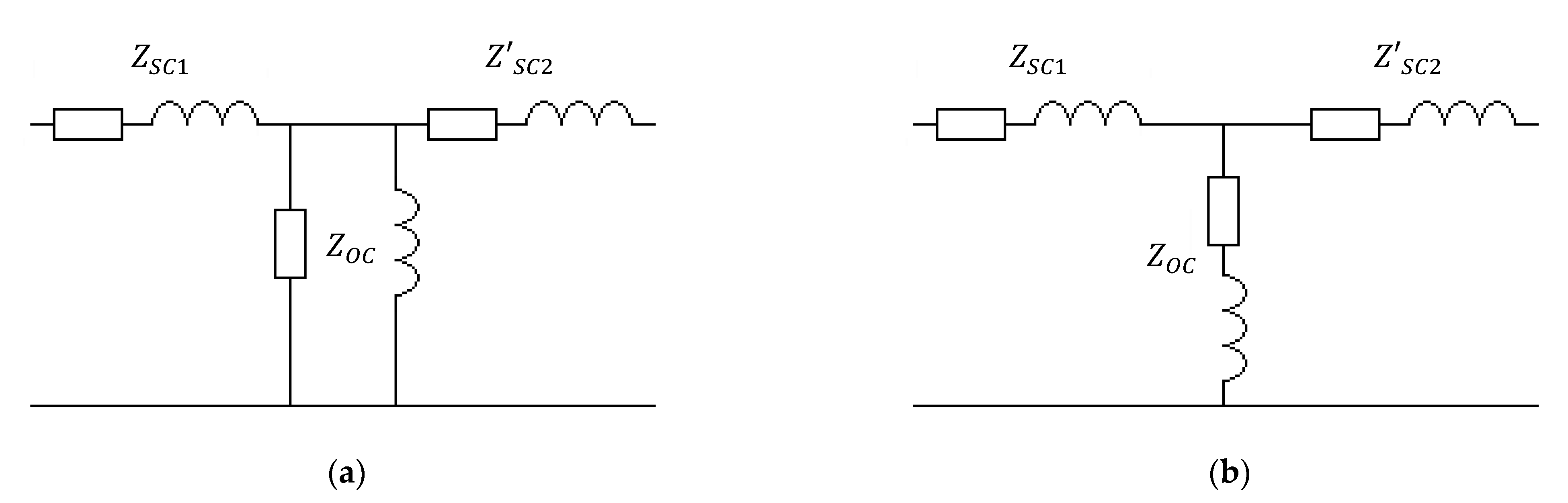
Cases of three-winding transformers and autotransformers are more complex. The equivalent circuit of a three-winding transformer is given in Figure A2a. In contrast, autotransformers have a different structure. An autotransformer’s primary winding is connected in parallel with the grid, the secondary is connected in series (Figure A2b) [58]. Both windings belong to the common coil and are linked not only magnetically, but also electrically. It is not an easy task to produce mathematical equations for an autotransformer, thus the equivalent scheme is rarely found in the literature. This procedure has been found in [73,74], and the scheme is given in Figure A2c. The interaction of a common coil with the tertiary winding can be regarded as a casual transformer with T-model since only the magnetic link is present. The winding configuration is Y0/Δ-1 [75].
For power transmission lines, the well-known models can be used—either the nominal Π-model (Figure A2d) or the distributed-element model (Figure A2e). The distributed element model, containing partial derivatives, is more complex, requires a longer computational time. Since the longest length in the test scheme is 100 km, the difference between simulation accuracies is not significant for this research. It is noteworthy that the phase velocity of the wave in the power transmission line depends on the product of inductance and capacitance [76,77]. The velocity must not be greater than the speed of light:
where: —the phase velocity, m/s; —the wavelength, m; —the period, s; —the line inductance per unit length, H/km; —the line capacitance per unit length, F/km; —the speed of light.
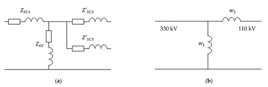
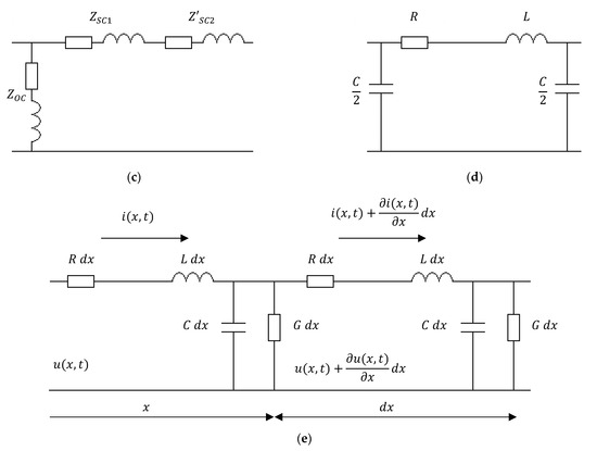
Figure A2.
(a) Equivalent circuit of a three-winding transformer with the magnetizing branch connected in series; (b) Scheme of a step-down autotransformer’s common winding connection to the grid; (c) Equivalent circuit of an autotransformer’s common winding; (d) Nominal Π-model of a transmission line; (e) Distributed-element model of a long transmission line.
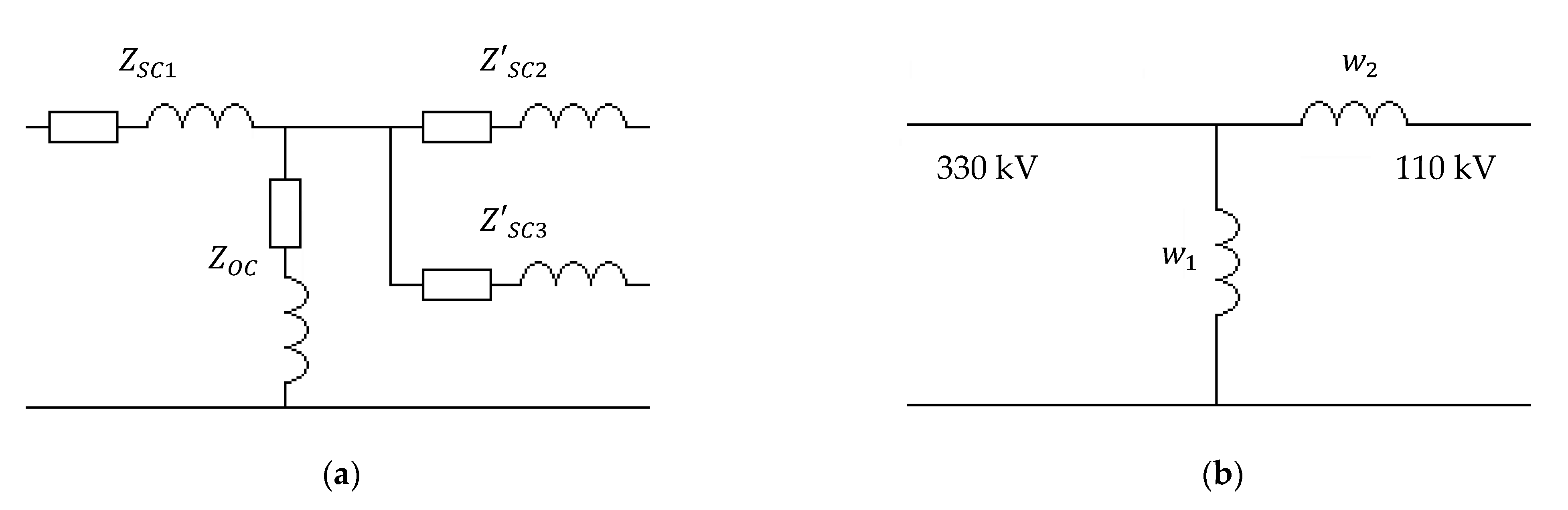

References
- IEEE Std 1159-2019; IEEE Recommended Practice for Monitoring Electric Power Quality. IEEE: New York, NY, USA, 2019.
- EN 50160:2010; Voltage Characteristics of Electricity Supplied by Public Electricity Networks. CENELEC: Brussels, Belgium, 2010.
- LST EN 61000-4-30:2015; Electromagnetic Compatibility (EMC)—Part 4-30: Testing and Measurement Techniques—PQ Measurement Methods (IEC 61000-4-30:2015). Lithuanian Standards Board: Vilnius, Lithuania, 2016.
- IEEE Std 1564-2014; IEEE Guide for Voltage Sag Indices. IEEE: New York, NY, USA, 2014.
- Liubčuk, V.; Radziukynas, V.; Naujokaitis, D.; Kairaitis, G. Grid Nodes Selection Strategies for Power Quality Monitoring. Appl. Sci. 2023, 13, 6048. [Google Scholar] [CrossRef]
- Ma, L.; Li, Y.; Tian, D.; Lou, J.; Chen, Y.; Liu, X. Assessment of Voltage Sag/Swell in the Distribution Network Based on Energy Index and Influence Degree Function. Electr. Power Syst. Res. 2023, 223, 109072. [Google Scholar] [CrossRef]
- Murray, R.L.; Keith, E.H. (Eds.) Chapter 21—Reactor Safety and Security: The Fukushima Daiichi Accident. In Nuclear Energy, 7th ed.; Butterworth-Heinemann: Oxford, UK, 2015; pp. 370–373. [Google Scholar]
- Fuchigami, M.; Kasahara, N. The Fukushima Nuclear Power Plant Accident: The Main Sequence of Events. In The 2011 Fukushima Nuclear Power Plant Accident; Hatamura, Y., Abe, S., Fuchigami, M., Kasahara, N., Eds.; Woodhead Publishing: Cambridge, UK, 2015; pp. 21–96. [Google Scholar]
- European Union. Commission Regulation (EU) 2016/631; Network Code on Requirements for Grid Connection of Generators. Off. J. Eur. Union 2016, 59, 1–68. Available online: http://data.europa.eu/eli/reg/2016/631/oj (accessed on 9 July 2023).
- Green Power Denmark. Guide for Connection of Power-Generating Plants to the Low-Voltage Grid (≤1 kV); Green Power Denmark: Copenhagen, Denmark, 2022; Available online: https://greenpowerdenmark.dk/files/media/document/Guide-for-grid-connection-of-demand-installations-to-the%20low-voltage-grid.pdf (accessed on 25 June 2023).
- Green Power Denmark. Guide for Connection of Power-Generating Plants to the Medium and High-Voltage Grid (>1 kV); Green Power Denmark: Copenhagen, Denmark, 2022; Available online: https://greenpowerdenmark.dk/files/media/document/Guide-to-grid-connection-of-demand-facilities-for-the-medium-and-high-voltage-grid_0.pdf (accessed on 25 June 2023).
- Stanelytė, D.; Radziukynas, V. Analysis of Voltage and Reactive Power Algorithms in Low Voltage Networks. Energies 2022, 15, 1843. [Google Scholar] [CrossRef]
- Tang, L.; Han, Y.; Yang, P.; Wang, C.; Zalhaf, A.S. A Review of Voltage Sag Control Measures and Equipment in Power System. Energy Rep. 2022, 8, 207–216. [Google Scholar] [CrossRef]
- Elphick, S.; Ciufo, P.; Drugy, G.; Smith, V.; Perera, S.; Gosbell, V. Large Scale Proactive Power-Quality Monitoring: An Example from Australia. IEEE Trans. Power Deliv. 2017, 32, 881–889. [Google Scholar] [CrossRef]
- De Santis, M.; Noce, C.; Varilone, P.; Verde, P. Analysis of the Origin of Measured Voltage Sags in Interconnected Networks. Electr. Power Syst. Res. 2018, 154, 391–400. [Google Scholar] [CrossRef]
- Mohammadi, Y.; Mohammad, H.M.; Leborgne, R.C. Locating the Source of Voltage Sags: Full Review, Introduction of Generalized Methods and Numerical Simulations. Renew. Sustain. Energy Rev. 2017, 27, 821–844. [Google Scholar] [CrossRef]
- Topolanek, D.; Lehtonen, M.; Adzman, M.R.; Toman, P. Earth Fault Location Based on Evaluation of Voltage Sag at Secondary Side of Medium Voltage/Low Voltage Transformers. IET Gen. Transm. Distrib. 2015, 9, 1801–2078. [Google Scholar] [CrossRef]
- Mohammadi, Y.; Moradi, M.H.; Leborgne, R.C. A Novel Method for Voltage-Sag Source Location Using a Robust Machine Learning Approach. Electr. Power Syst. Res. 2017, 145, 122–136. [Google Scholar] [CrossRef]
- Chang, W.G.; Chao, J.; Hunter, M.H.; Chen, C.; Chu, S. On Tracking the Source Location of Voltage Sags and Utility Shunt Capacitor Switching Transients. IEEE Trans. Power Deliv. 2008, 23, 2124–2131. [Google Scholar] [CrossRef]
- Won, D.; Moon, S. Topological Locating of Power Quality Events Source. Electr. Eng. Technol. 2006, 1, 170–176. [Google Scholar] [CrossRef]
- Mohammad, H.M.; Mohammadi, Y. Voltage Sag Source Location: A Review with Introduction of a New Method. Electr. Power Energy Syst. 2012, 43, 29–39. [Google Scholar]
- Zhang, X.; Xu, Y.H. Analysis of Voltage Sag Source Location Based on Wavelet-Multiresolution Method. In Proceedings of the APPEEC 2010, Chengdu, China, 28–31 March 2010. [Google Scholar]
- Wang, B.; Xu, W.; Pan, Z. Voltage Sag State Estimation for Power Distribution Systems. IEEE Trans. Power Syst. 2005, 20, 806–812. [Google Scholar] [CrossRef]
- Shao, Z.; Peng, J.; Kang, J. Locating Voltage Sag Source with Impedance Measurement. In Proceedings of the POWERCON 2010, Zhejiang, China, 24–28 October 2010. [Google Scholar]
- Mohammadi, Y.; Leborgne, R.C. A New Approach for Voltage Sag Source Relative Location in Active Distribution Systems with the Presence of Inverter-Based Distributed Generations. Electr. Power Syst. Res. 2020, 182, 106222. [Google Scholar] [CrossRef]
- Mohammadi, Y.; Leborgne, R.C. Improved DR and CBM Methods for Finding Relative Location of Voltage Sag Source at the PCC of Distributed Energy Resources. Electr. Power Energy Syst. 2020, 117, 105644. [Google Scholar] [CrossRef]
- Yi, T.; Jie, H.; Hao, L.; Lei, W. Method for Voltage Sag Source Location Based on the Internal Resistance Sign in a Single-Port Network. IET Gen. Transm. Distrib. 2016, 10, 1495–1767. [Google Scholar] [CrossRef]
- Zhu, K.; Wang, Y.; Yin, P.; Ni, J. Voltage Sag Source Location Technology Based on Corresponding Sequence Components. IET Gen. Transm. Distrib. 2014, 9, 789–883. [Google Scholar] [CrossRef]
- Tayjasanant, T.; Li, C.; Xu, W. A Resistance Sign-Based Method for Voltage Sag Source Detection. IEEE Trans. Power Deliv. 2005, 20, 2544–2551. [Google Scholar] [CrossRef]
- Shareef, H.; Mohamed, A.; Ibrahim, A.A. Identification of Voltage Sag Source Location Using S and TT Transformed Disturbance Power. Central South Univ. 2013, 20, 83–97. [Google Scholar] [CrossRef]
- Polajžer, B.; Štrumberger, G.; Seme, S.; Dolinar, D. Detection of Voltage Sag Sources Based on Instantaneous Voltage and Current Vectors and Orthogonal Clarke’s Transformation. IET Gen. Transm. Distrib. 2008, 2, 219–226. [Google Scholar] [CrossRef]
- Polajžer, B.; Štrumberger, G.; Dolnar, D. Instantaneous Positive-Sequence Current Applied for Detecting Voltage Sag Sources. IET Gen. Transm. Distrib. 2015, 9, 307–403. [Google Scholar] [CrossRef]
- Liu, Z.; Zhang, S.; Li, W.; Zheng, C.; Liu, S.; Wang, L. Voltage Sag Source Location Based on Sag Event Amplitude Information. In Proceedings of the CFEEE 2022, Beihai, China, 16–18 December 2022. [Google Scholar]
- Bollen, M.; Baumann, P.; Beyer, Y.; Castel, R.; Esteves, J.; Faias, S.; Friedl, W.; Larzeni, S.; Trhulj, J.; Villa, F.; et al. Guidelines for Good Practice on Voltage Quality Monitoring. In Proceedings of the 22nd CIRED, Stockholm, Sweden, 10–13 June 2013. [Google Scholar]
- Ibrahim, A.; Mohamed, A.; Shareef, H.; Ghoshal, P. A New Approach for Optimal Power Quality Monitor Placement in Power System Considering System Topology. Przeglad Elektrotechn. 2012, 9, 272–276. [Google Scholar]
- Branco, H.M.G.C.; Oleskovicz, M.; Delbem, A.C.B.; Coury, D.V.; Silva, R.P.M. Optimized Allocation of Power Quality Monitors in Transmission Systems: A Multi-objective Approach. Electr. Power Energy Syst. 2015, 64, 156–166. [Google Scholar] [CrossRef]
- Branco, H.M.G.C.; Oleskovicz, M.; Coury, D.V.; Delbem, A.C.B. Multi-Objective Optimization for Power Quality Monitoring Allocation Considering Voltage Sags in Distribution Systems. Electr. Power Energy Syst. 2018, 97, 1–10. [Google Scholar] [CrossRef]
- Martins, P.E.T.; Zvietcovich, W.G.; De Oliveira Silva, T.A.; De Oliveira, F.B. Multi-Objective Approach for Power Quality Monitor Allocation with Symmetry in Short-Duration Voltage Variations. IEEE Trans. Power Deliv. 2019, 34, 430–437. [Google Scholar] [CrossRef]
- Martins, P.E.T.; Oleskovicz, M. Multi-Objective Optimization Aiming to Minimize the Number of Power Quality Monitors and Multiple Fault Estimations in Unbalanced Power Distribution System. In Proceedings of the 20th ICHQP, Naples, Italy, 29 May–1 June 2022. [Google Scholar]
- Kempner, T.R.; Oleskovicz, M.; Gomes, D.P. Optimal Monitoring of Voltage Sags Through Simultaneous Analysis of Short-Circuits in Distribution Systems. IET Gener. Transm. Distrib. 2017, 11, 1801–1808. [Google Scholar] [CrossRef]
- Kazemi, A.; Mohamed, A.; Shareef, H.; Zayandehroodi, H. Optimal Power Quality Monitor Placement Using Genetic Algorithm and Mallow’s Cp. Electr. Power Energy Syst. 2013, 53, 564–575. [Google Scholar] [CrossRef]
- Tan, M.; Zhang, C.; Chen, B. Configuration of Power Quality Monitor Considering Voltage Sag Location. Electr. Power Sys. Res. 2023, 223, 109681. [Google Scholar] [CrossRef]
- Chiumeo, R.; Porrino, A.; Garbero, L.; Tenti, L.; Nigris, M. The Italian Power Quality Monitoring System of the MV Network Results of the Measurements of Voltage Dips after 3 Years Campaign. In Proceedings of the 20th CIRED, Prague, Czech Republic, 8–11 June 2009. [Google Scholar]
- Salora, Ö.; Buhana, S.; Ünsar, Ö.; Bovrazoglu, B.; Altintas, A.; Atalik, T.; Haliloglu, B.; Inan, T.; Kalavcioglu, A.; Terciyanli, A.; et al. Mobile Monitoring System to Take Nationwide PQ Measurements on Electricity Transmission System. Measurement 2009, 42, 501–515. [Google Scholar] [CrossRef]
- Vinnal, T.; Jarkovoi, M.; Kütt, L. Voltage Dips and Swells in Low Voltage Network of Estonia. In Proceedings of the 59th RTUCON, Riga, Latvia, 12–13 November 2018. [Google Scholar]
- Freitas, A.F.; Amaral, F.V.; Silva, J.A.L.; Saldanha, R.R.; Silva, S.M. Optimum Allocation of Power Quality Monitors in Electric Power Systems—A Case Study. In Proceedings of the 17th ICHQP, Belo Horizonte, Brazil, 16–19 October 2016. [Google Scholar]
- Carpinelli, G.; Di Perna, C.; Caramia, P.; Varilone, P.; Verde, P. Methods for Assessing the Robustness of Electrical Power Systems Against Voltage Dips. IEEE Trans. Power Deliv. 2009, 24, 43–51. [Google Scholar] [CrossRef]
- Council of European Energy Regulators. 5th CEER Benchmarking Report on the Quality of Electricity and Gas Supply; CEER: Brussels, Belgium, 2011. [Google Scholar]
- Council of European Energy Regulators. 6th CEER Benchmarking Report on the Quality of Electricity and Gas Supply; CEER: Brussels, Belgium, 2016. [Google Scholar]
- Council of European Energy Regulators. 7th CEER Benchmarking Report on the Quality of Electricity and Gas Supply; CEER: Brussels, Belgium, 2022. [Google Scholar]
- Feng, D.; Wang, T.; Ying-Ying, L.; Zhou, S.; Li, Y. A New Method for Allocation of Power Quality Monitoring Sites. In Proceedings of the 9th IPEMC2020-ECCE Asia, Nanjing, China, 29 November–2 December 2020. [Google Scholar]
- IEEE Std 1366-2022; IEEE Guide for Electric Power Distribution Reliability Indices. IEEE: New York, NY, USA, 2022.
- Heylen, E.; De Boeck, S.; Ovaere, M.; Ergun, H.; Van Hertem, D. Steady-State Security. In Dynamic Vulnerability Assessment and Intelligent Control for Sustainable Power Systems; John Wiley & Sons: Hoboken, NJ, USA, 2018; pp. 21–40. [Google Scholar]
- Carvallo, J.P.; Frick, N.M.; Schwartz, L. A Review of Examples and Opportunities to Quantify the Grid Reliability and Resilience Impacts of Energy Efficiency. Energy Pol. 2022, 169, 113185. [Google Scholar] [CrossRef]
- Пoлoвкo, A.M. Ocнoвы Teopии Haдeжнocти; «Hayкa»: Moscow, Russia, 1964. [Google Scholar]
- Navickas, A. Elektros Energetikos Sistemų Patikimumas; Kaunas University of Technology—Publishing House “Technologija”: Kaunas, Lithuania, 2007. [Google Scholar]
- Kemabonta, T.; Mowry, G. A Syncretistic Approach to Grid Reliability and Resilience: Investigations from Minnesota. Energy Strat. Rev. 2021, 38, 100726. [Google Scholar] [CrossRef]
- Boльдeк, A.И. Элeктpичecкиe Maшины, 3rd ed.; Toлвинcкaя, E.B., Ed.; «Энepгия»: Leningrad, Russia, 1978. [Google Scholar]
- Блoк, B.M. , Oбyшeв, Г.K., Пaпepнo, Л.Б., Гyceвa, C.A., Гepxapд, Я.X. Пocoбиe к Kypcoвoмy и Диплoмнoмy Пpoeктиpoвaнию для Элeктpoэнepгeтичecкиx Cпeциaльнocтeй: Учeбнoe Пocoбиe для Cтyдeнтoв Byзoв; «Bыcшaя шкoлa»: Moscow, Russia, 1981. [Google Scholar]
- Svinkūnas, G.; Navickas, A. Elektros Energetikos Pagrindai, 2nd ed.; Kaunas University of Technology—Publishing House “Technologija”: Kaunas, Lithuania, 2013. [Google Scholar]
- Douglas, C.M.; George, C.R. Statistical Intervals for a Single Sample. In Applied Statistics and Probability for Engineers, 3rd ed.; John Wiley & Sons: New York, NY, USA, 2003; pp. 247–326. [Google Scholar]
- Johnson, N.L.; Kemp, A.W.; Kotz, S. Univariate Discrete Distributions, 3rd ed.; John Wiley & Sons: Hoboken, NJ, USA, 2005. [Google Scholar]
- World Nuclear Association. Nuclear Power in Lithuania. Available online: https://www.world-nuclear.org/information-library/country-profiles/countries-g-n/lithuania.aspx (accessed on 12 August 2023).
- Greenland, S.; Senn, S.J.; Rothman, K.J.; Carlin, J.B.; Poole, C.; Goodman, S.N.; Altman, D.G. Statistical Tests, P Values, Confidence Intervals, and Power: A Guide to Misinterpretations. Eur. J. Epidemiol. 2016, 31, 337–350. [Google Scholar] [CrossRef] [PubMed]
- Kalinowski, P. Identifying Misconceptions about Confidence Intervals. In Proceedings of the 8th ICOTS, Ljubljana, Slovenia, 11–16 July 2010. [Google Scholar]
- Baublys, J.; Jankauskas, P.; Marckevičius, L.A.; Morkvėnas, A. Izoliacija ir Viršįtampiai; Kaunas University of Technology—Publishing House “Technologija”: Kaunas, Lithuania, 2008. [Google Scholar]
- IEEE Std 998-2012; IEEE Guide for Direct Lightning Stroke Shielding of Substations. IEEE: New York, NY, USA, 2013.
- Milanović, J.V.; Meyer, J.; Ball, R.F.; Howe, W.; Preece, R.; Bollen, M.H.J.; Elphick, S.; Cukalevski, N. International Industry Practice on Power Quality Monitoring. IEEE Trans. Power Deliv. 2014, 29, 934–941. [Google Scholar] [CrossRef]
- Paltanavičius, S. Paukščiai ir Aukštosios Įtampos Linijos. Kada Gyventi Saugu? “Lututė”: Kaunas, Lithuania, 2015. [Google Scholar]
- Installation of the Bird Protection Measures on the High Voltage Electricity Transmission Grid in Lithuania. Final Report. 2019. Available online: http://www.birds-electrogrid.lt/news/159/208/European-Commission-has-approved-the-final-LIFE-Birds-on-Electrogrid-report/d,detalus-en/ (accessed on 4 September 2023).
- Lithuanian Ornithological Society. Call for Information on Birds Killed by Collision with Power Lines. Available online: https://www.birdlife.lt/kvieciame-teikti-informacija-apie-nuo-susidurimo-s (accessed on 3 September 2023).
- Khokhar, S.B.; Mohn Zin, A.A.B.; Mokhtar, A.S.B.; Pesaran, M. A Comprehensive Overview on Signal Processing and Artificial Intelligence Techniques Applications in Classification of Power Quality Disturbances. Renew. Sustain. Energy Rev. 2015, 51, 1650–1663. [Google Scholar] [CrossRef]
- YouTube. Autotransformer Equivalent Circuit [Video]. Available online: https://www.youtube.com/watch?v=DRRwWSPEjz0 (accessed on 24 June 2023).
- YouTube. Equivalent Circuit of Autotransformer [Video]. Available online: https://www.youtube.com/watch?v=-O6_78sp3KM (accessed on 24 June 2023).
- MathWorks. Help Center. Three-Phase Autotransformer with Tertiary Winding. Available online: https://www.mathworks.com/help/sps/powersys/ref/threephaseautotransformerwithtertiarywinding.html (accessed on 25 June 2023).
- MathWorks. Help Center. Distributed Parameters Line. Available online: https://www.mathworks.com/help/sps/powersys/ref/distributedparametersline.html (accessed on 27 June 2023).
- Pukys, P. Teorinė Elektrotechnika II, 4th ed.; Bartkevičius, S., Lazauskas, V., Pukys, P., Stonys, J., Virbalis, A., Eds.; Kaunas University of Technology—Publishing House “Technologija”: Kaunas, Lithuania, 2011. [Google Scholar]
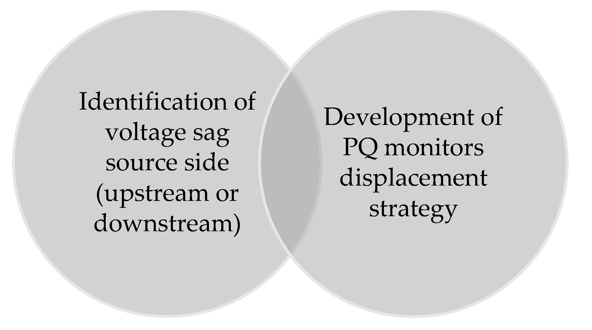
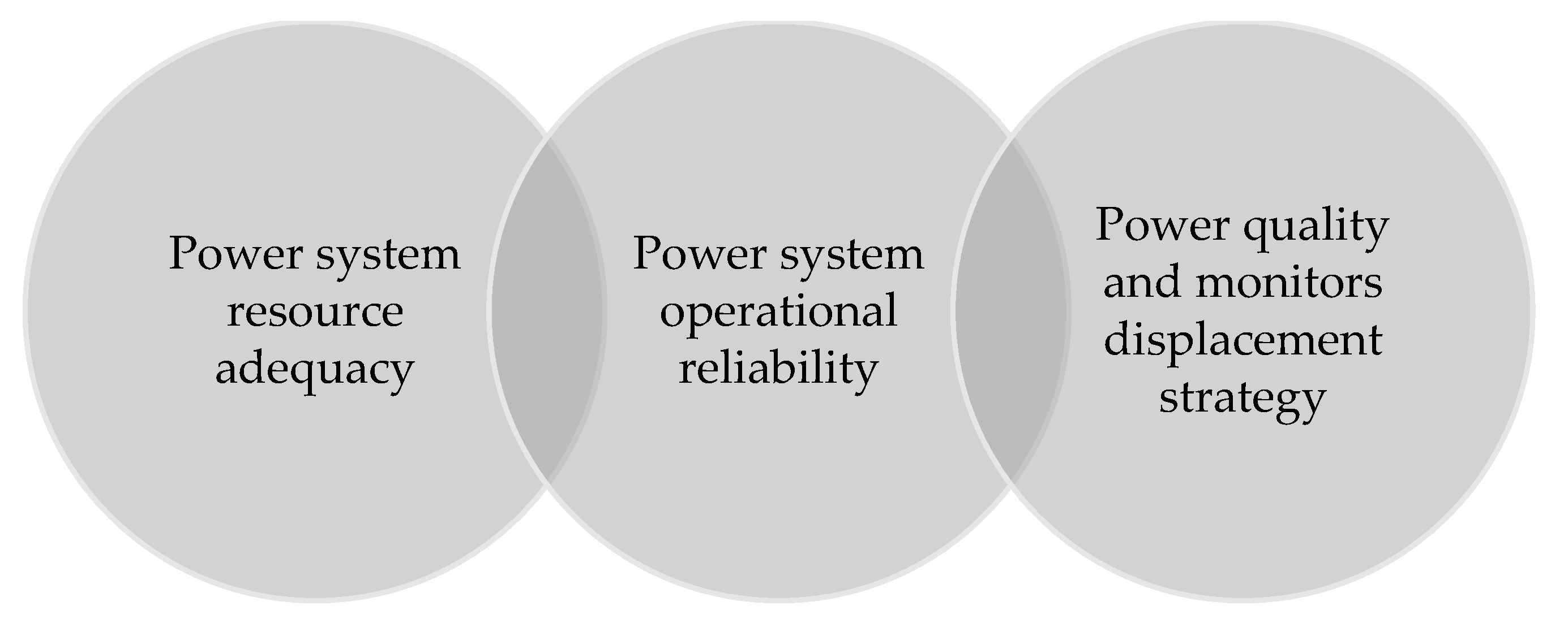
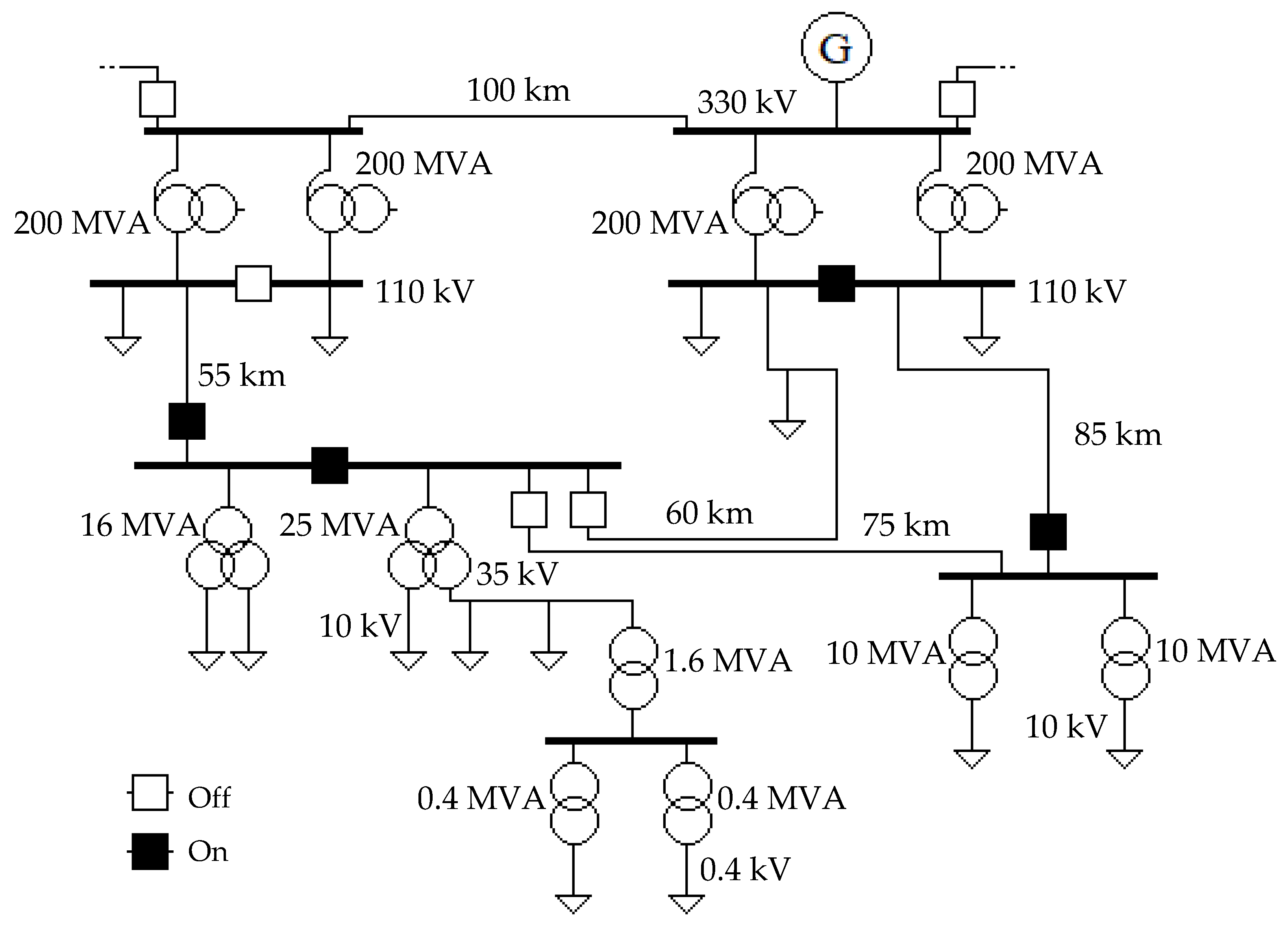
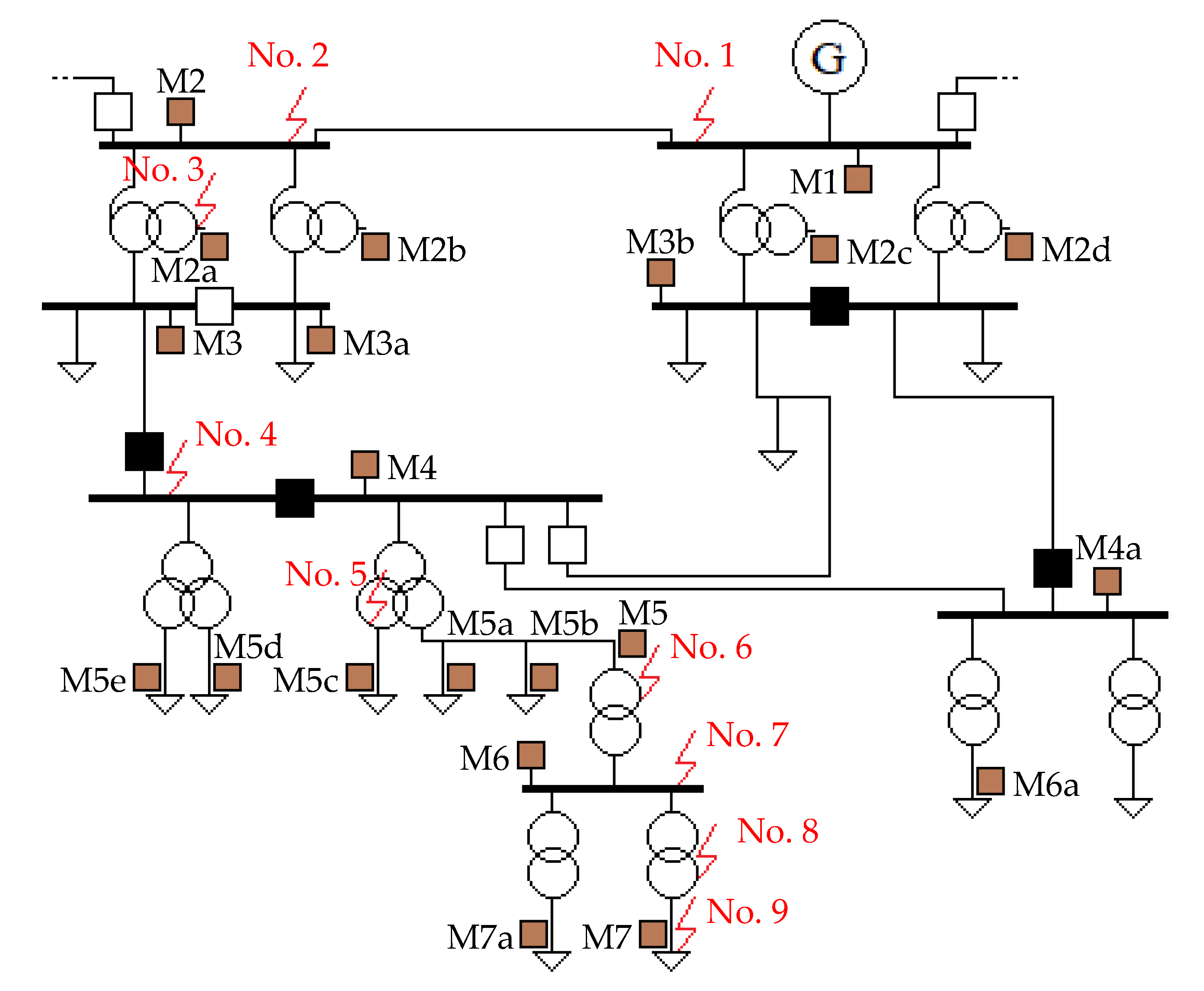
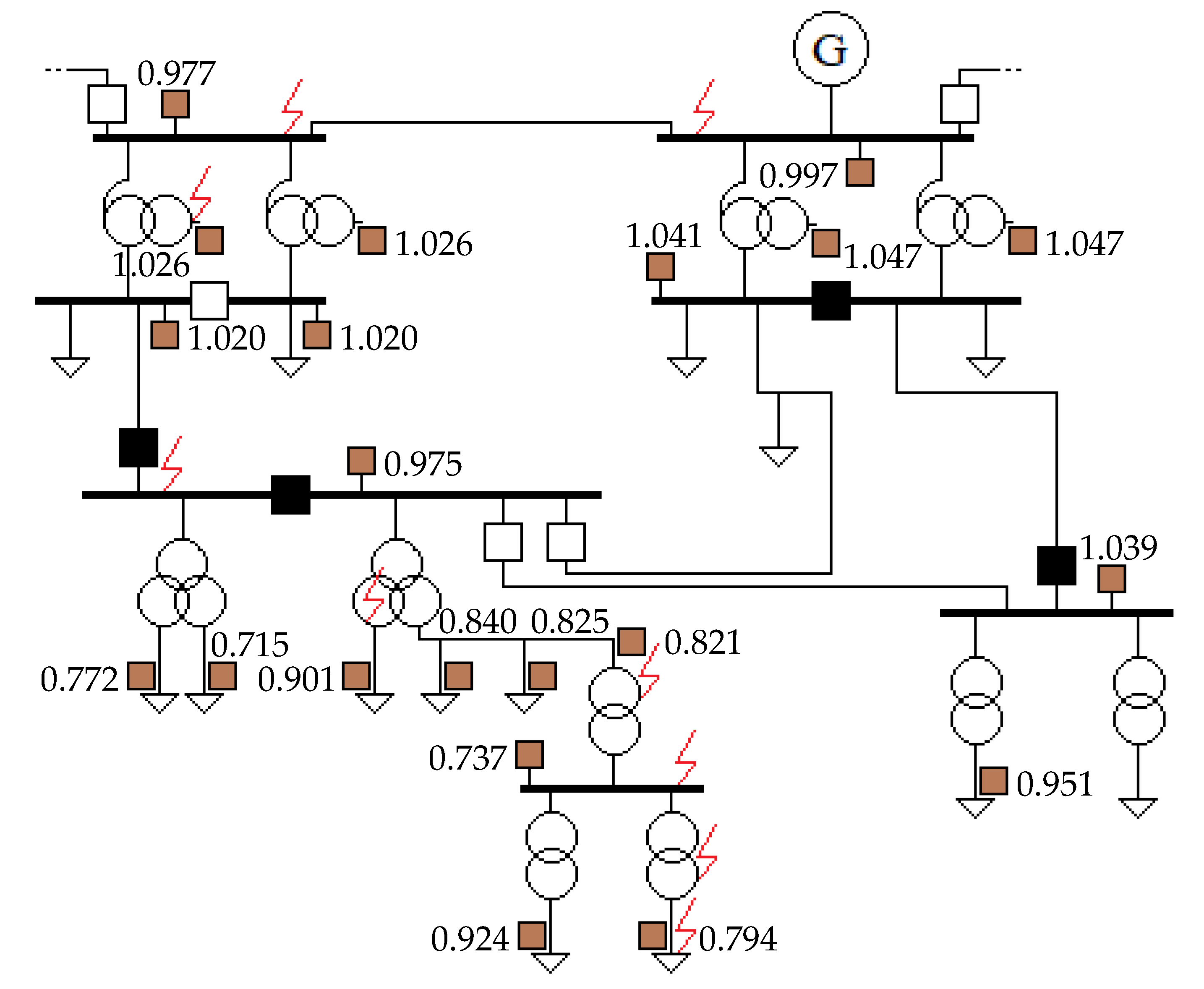
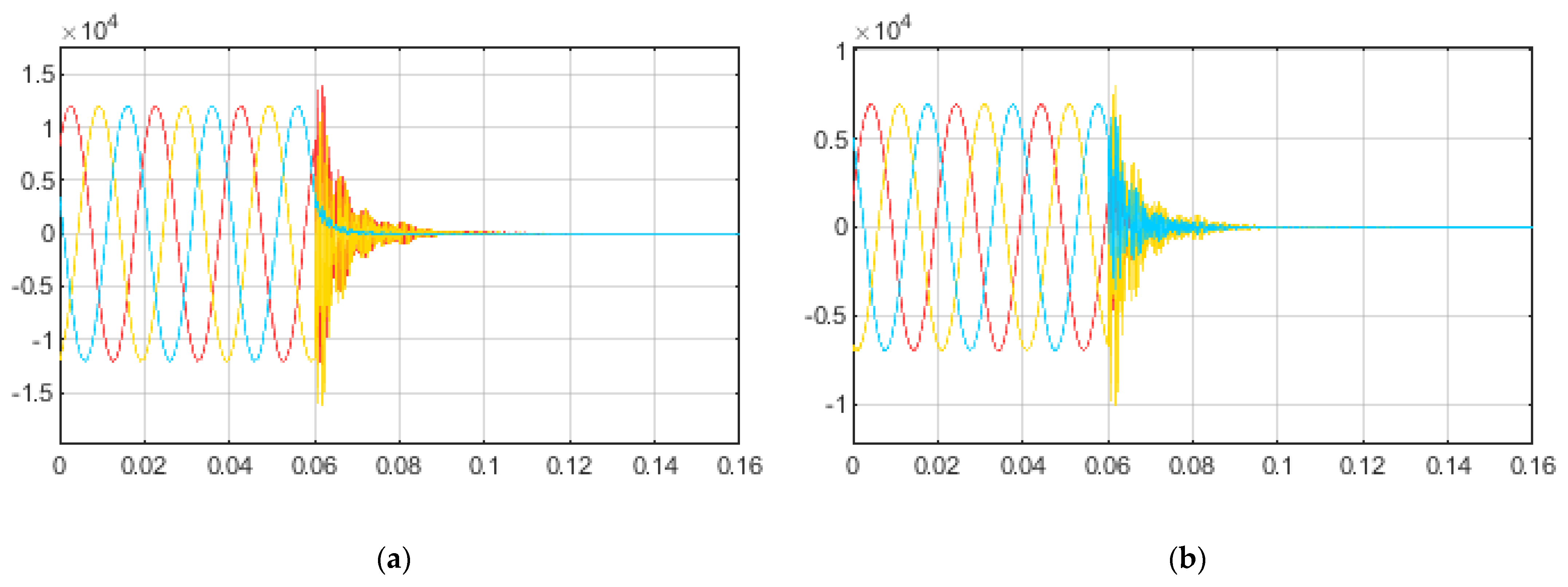
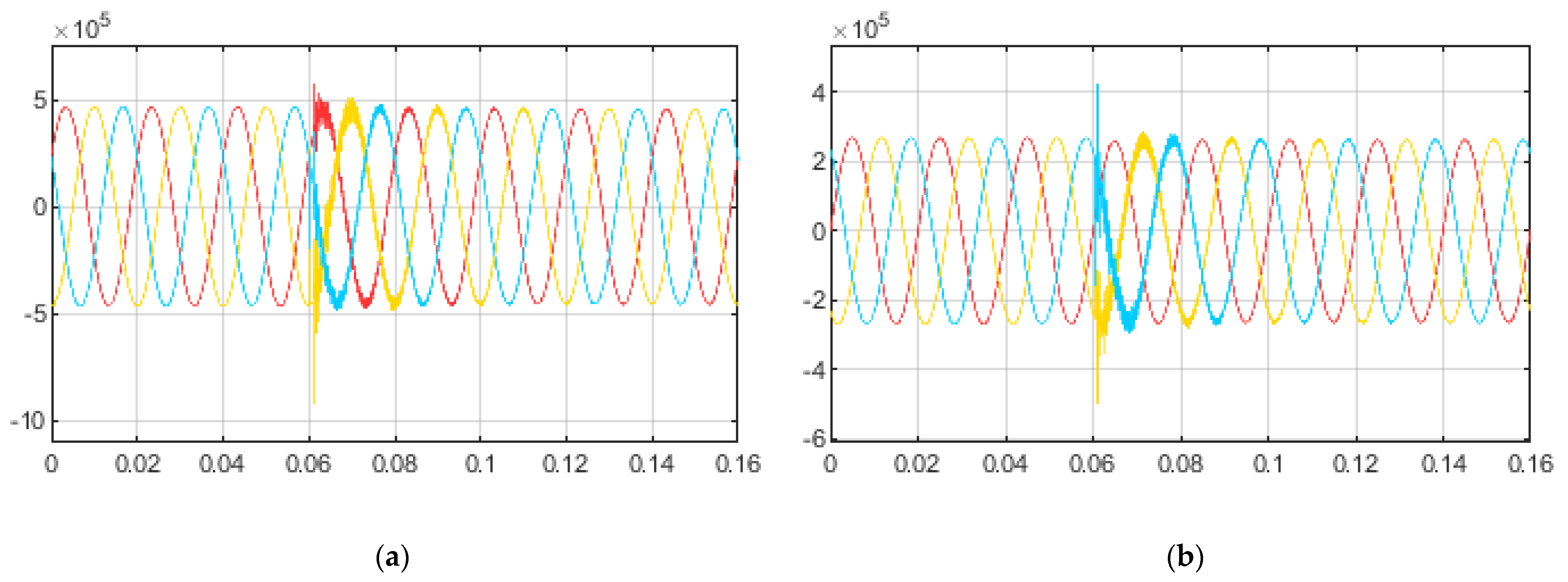
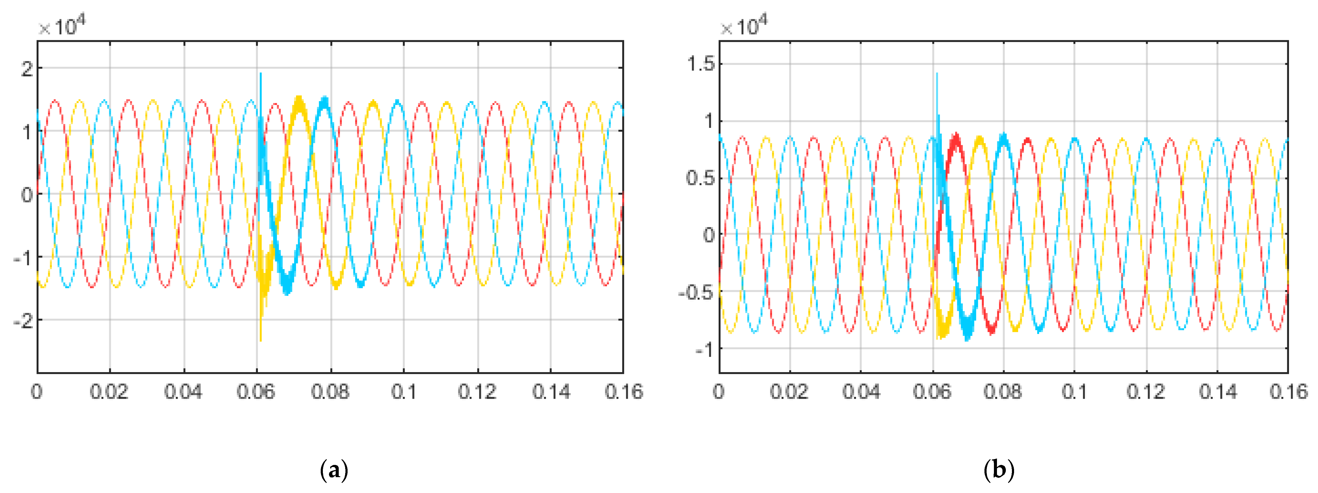
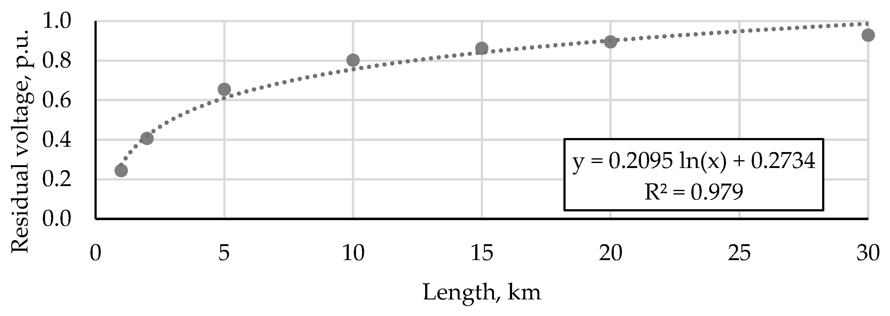
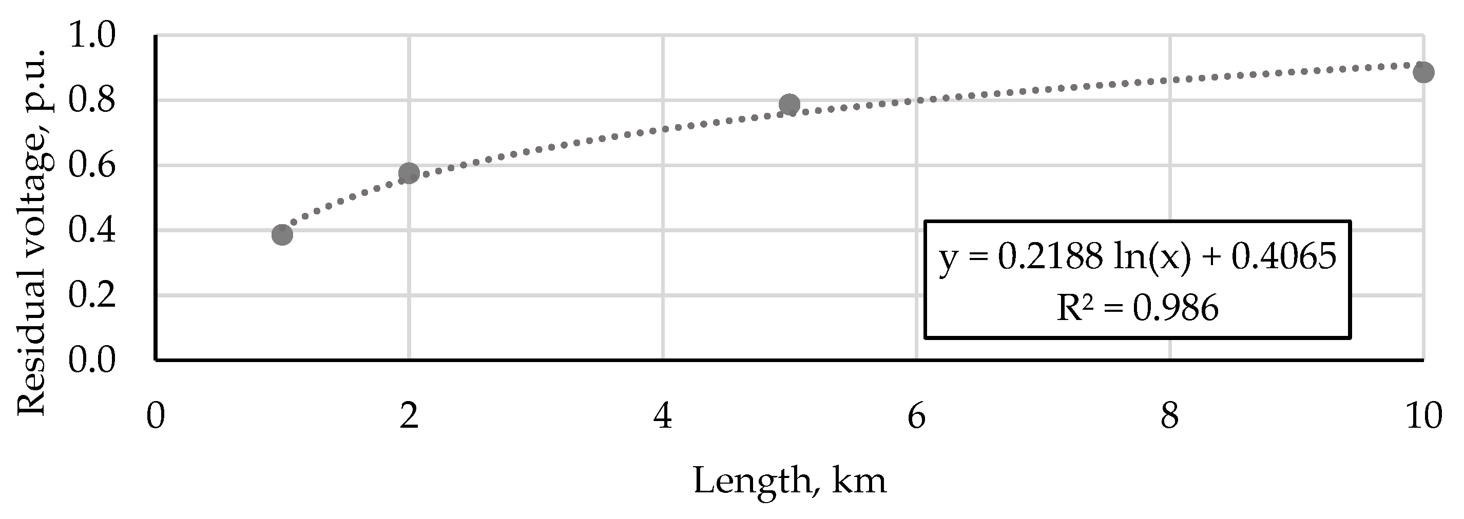
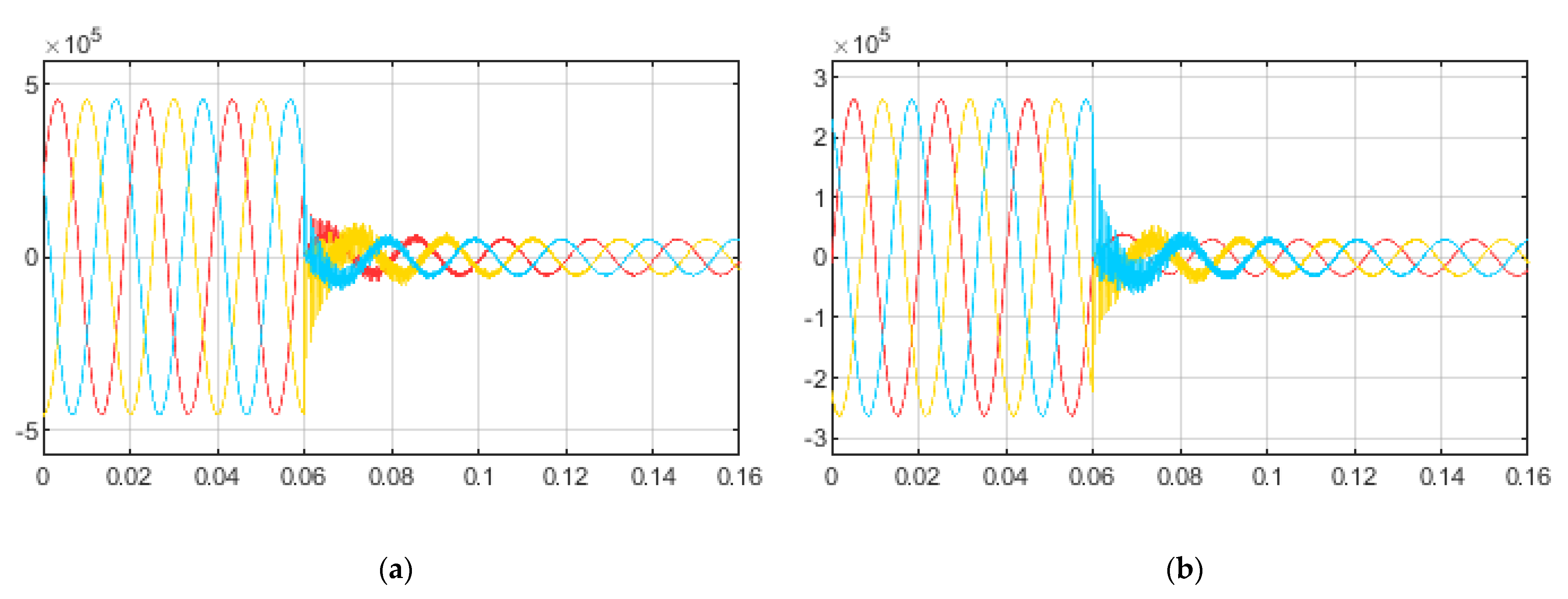
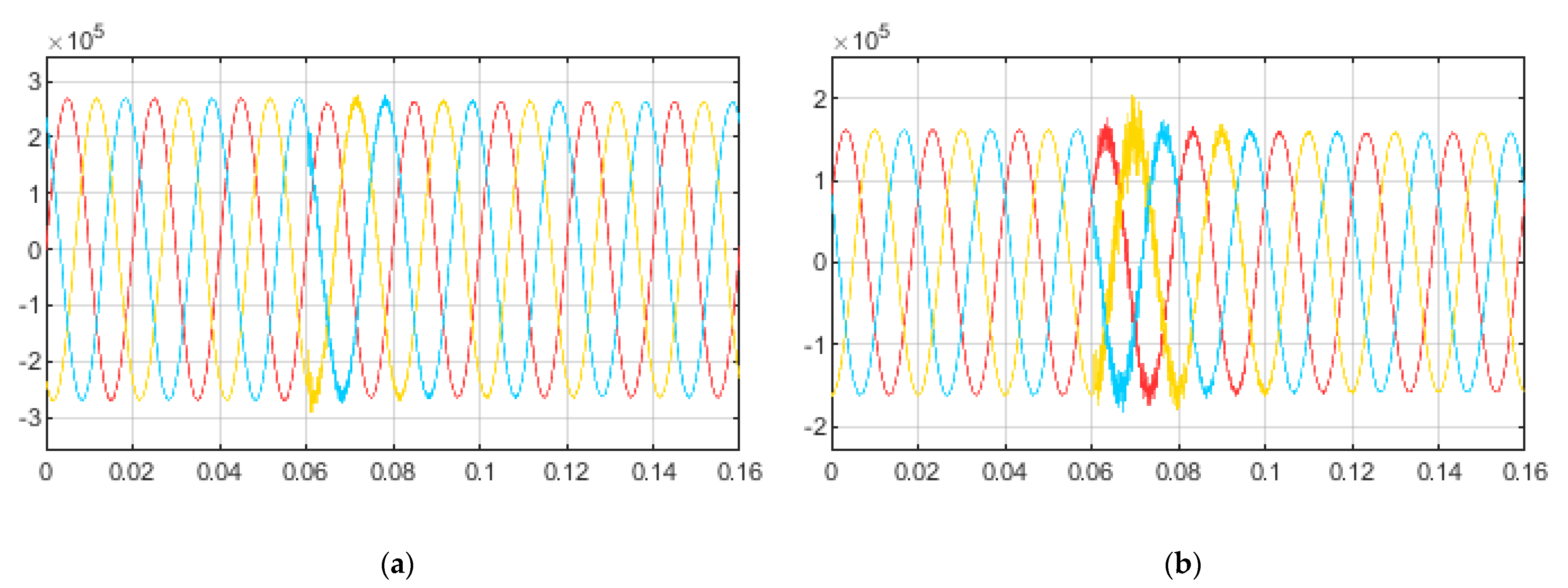
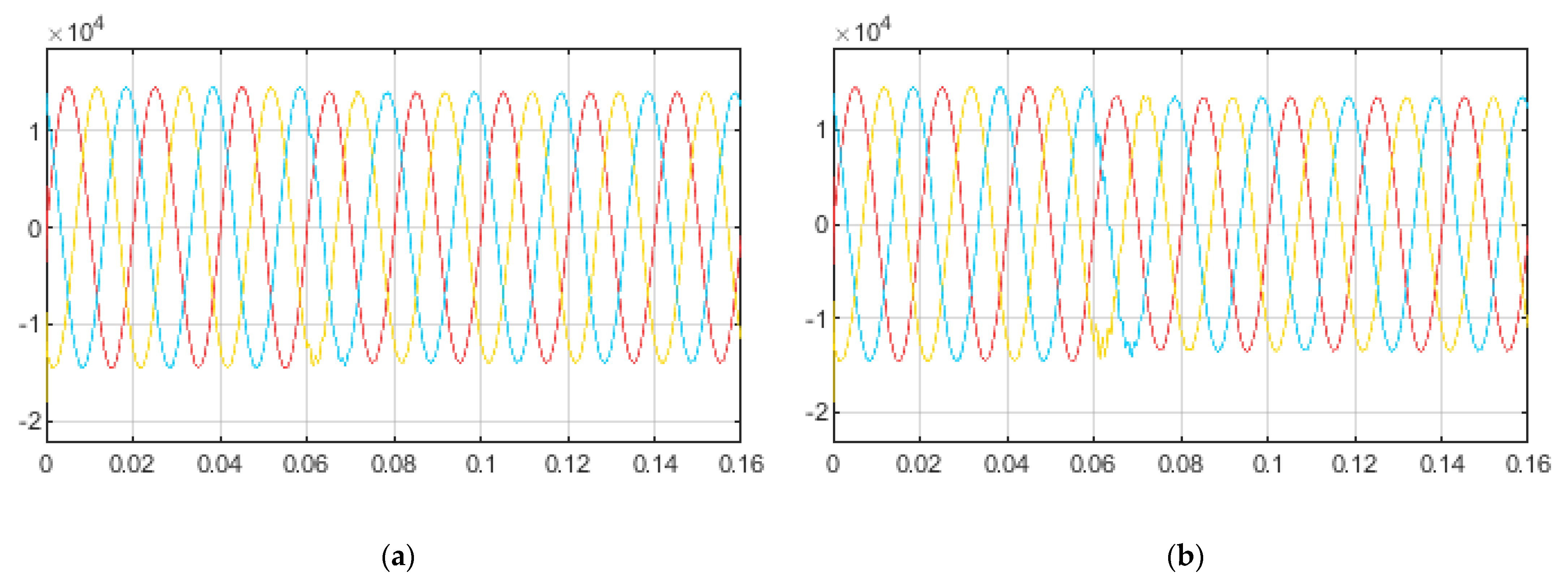
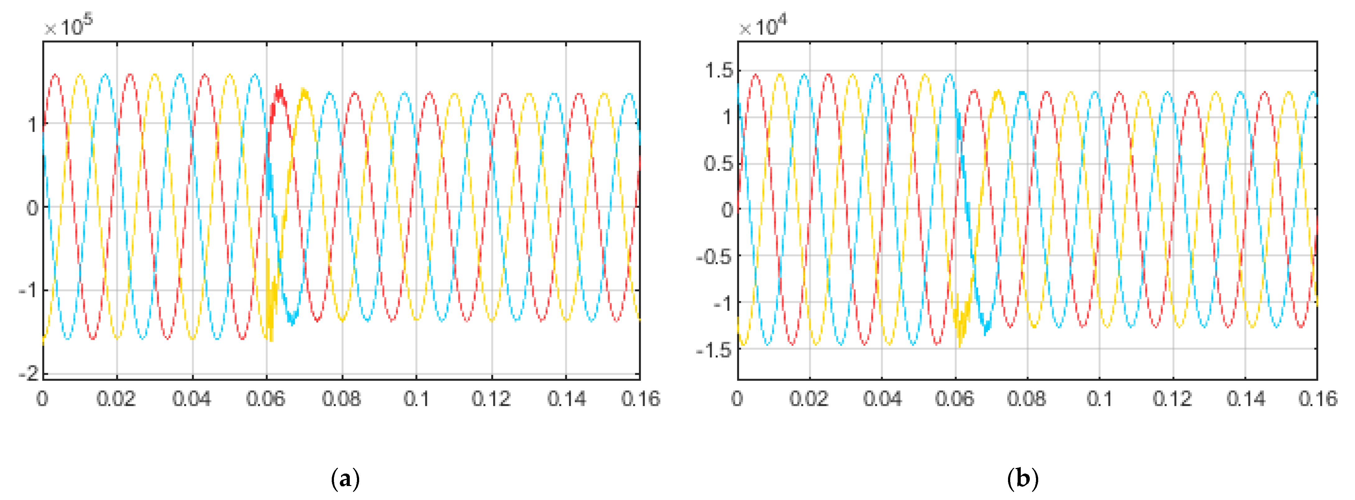
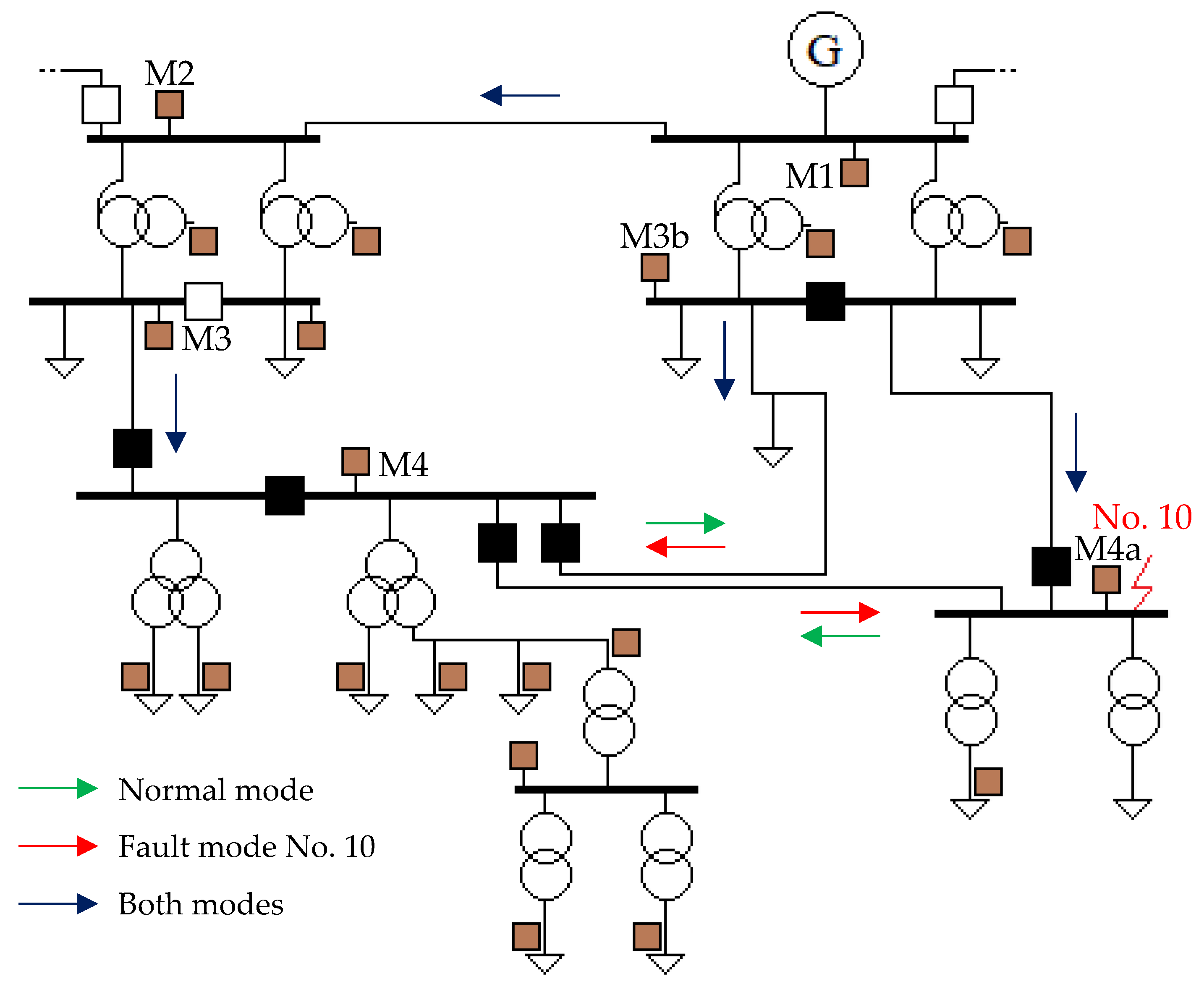
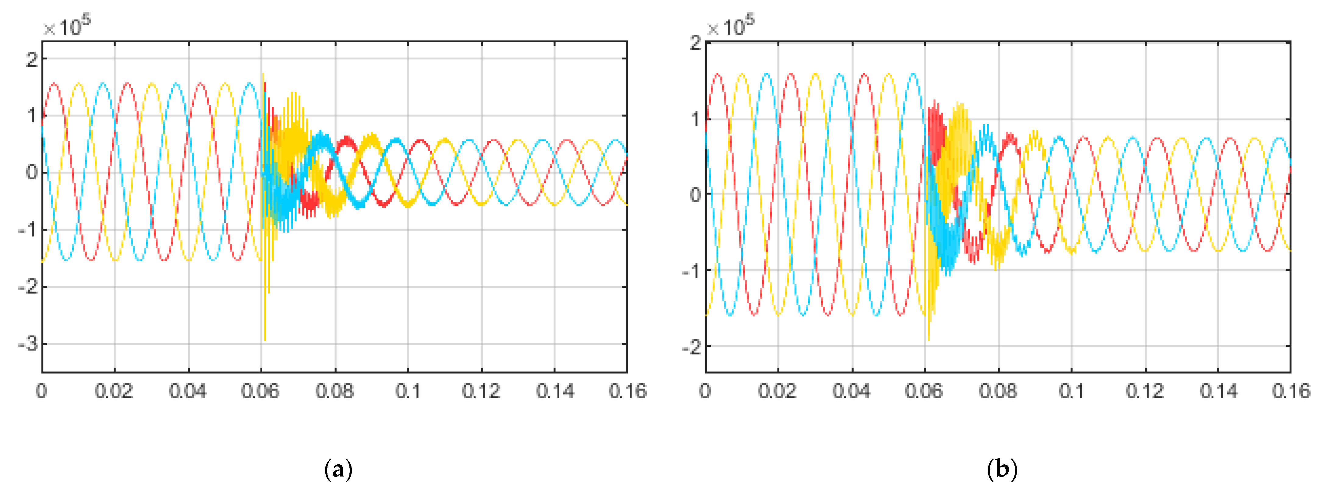
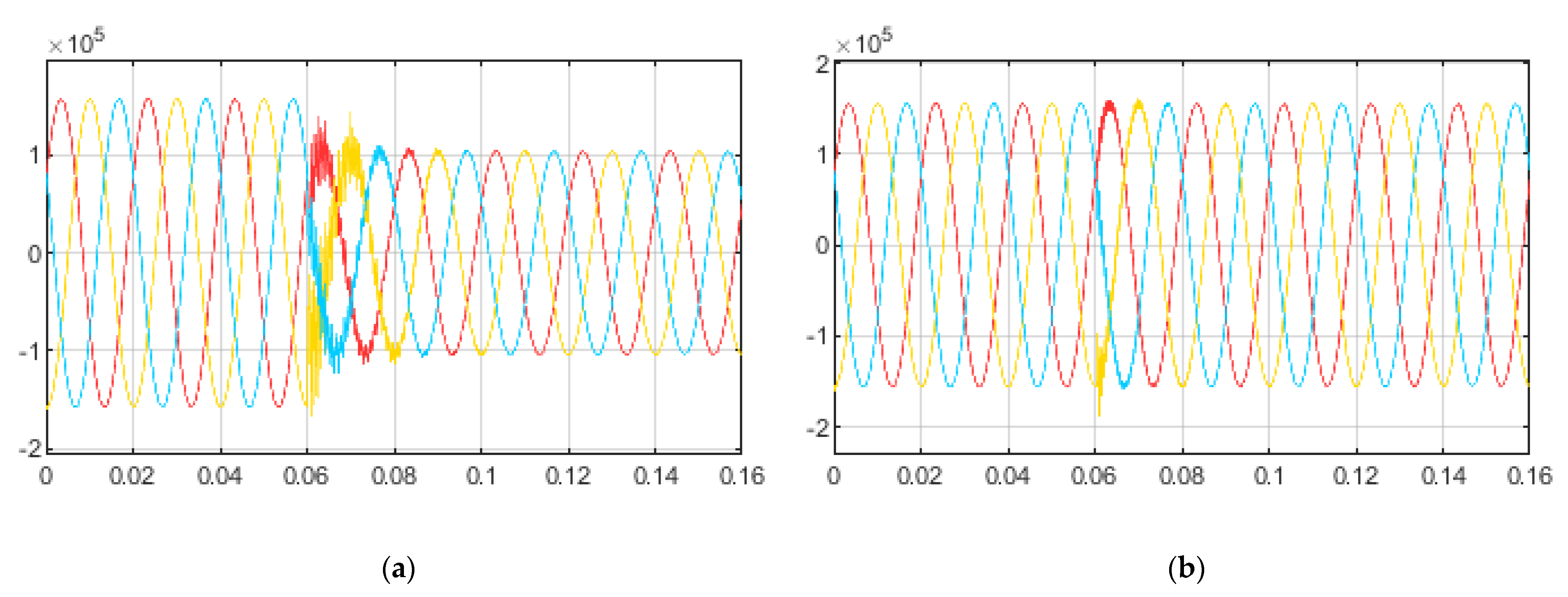
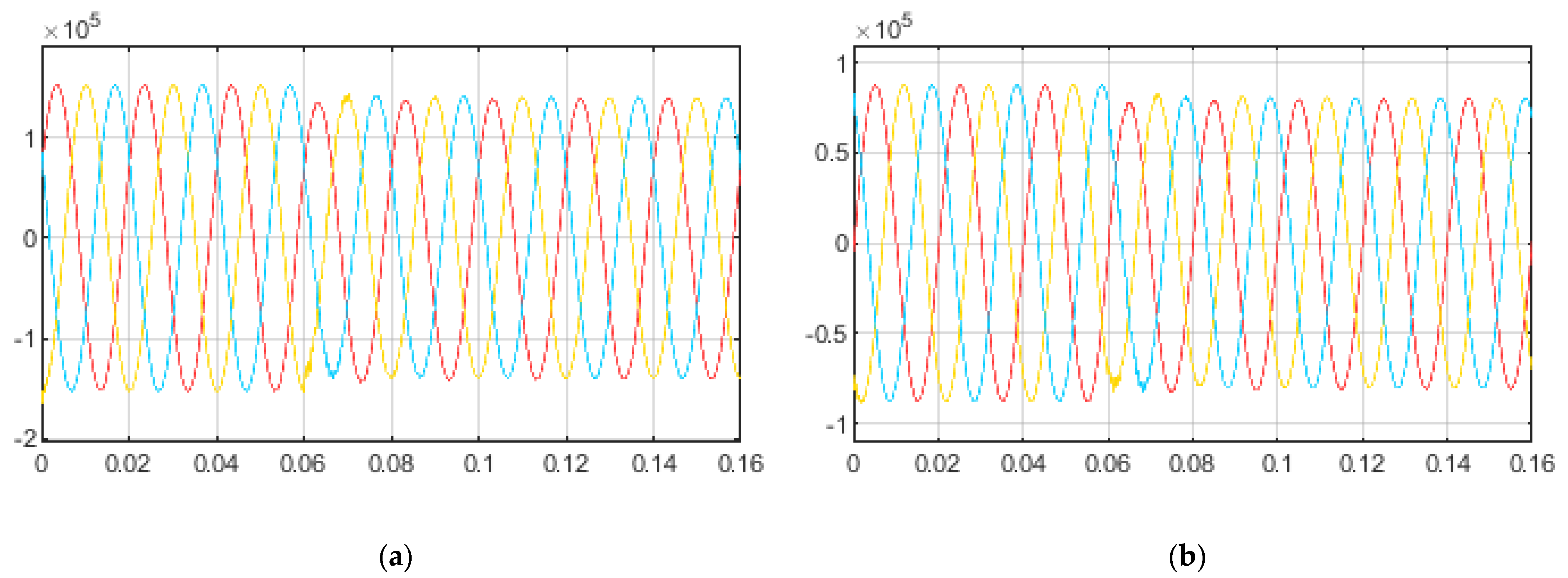
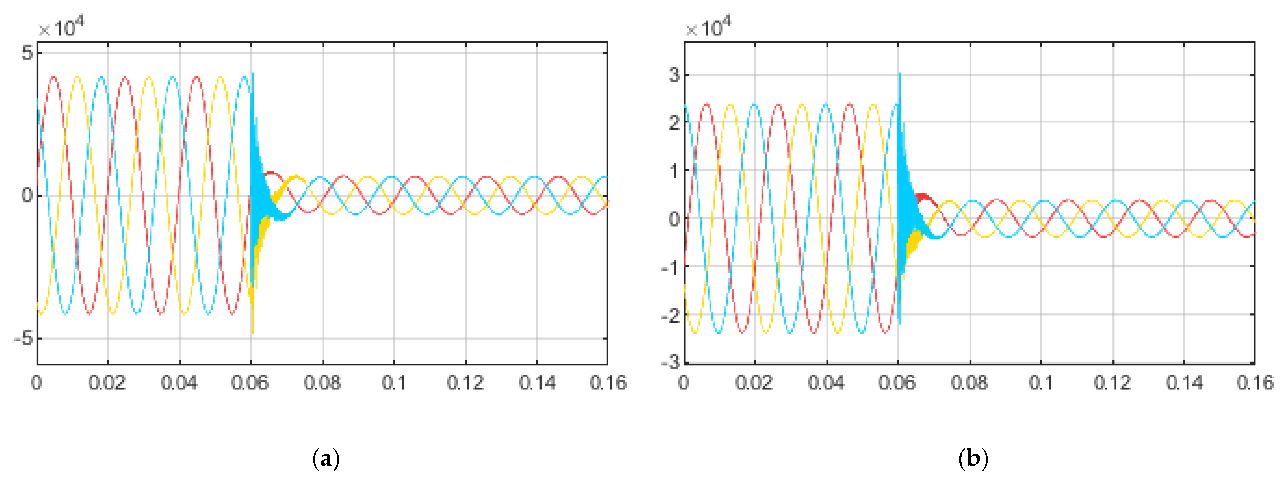
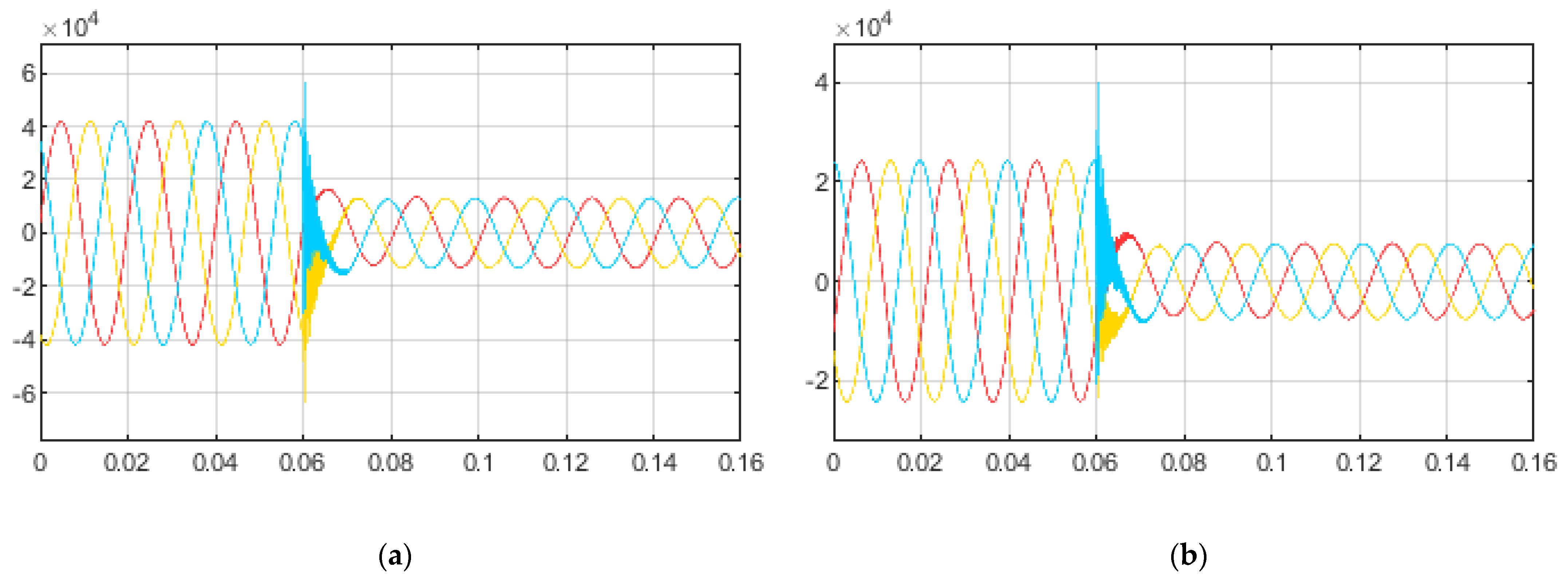
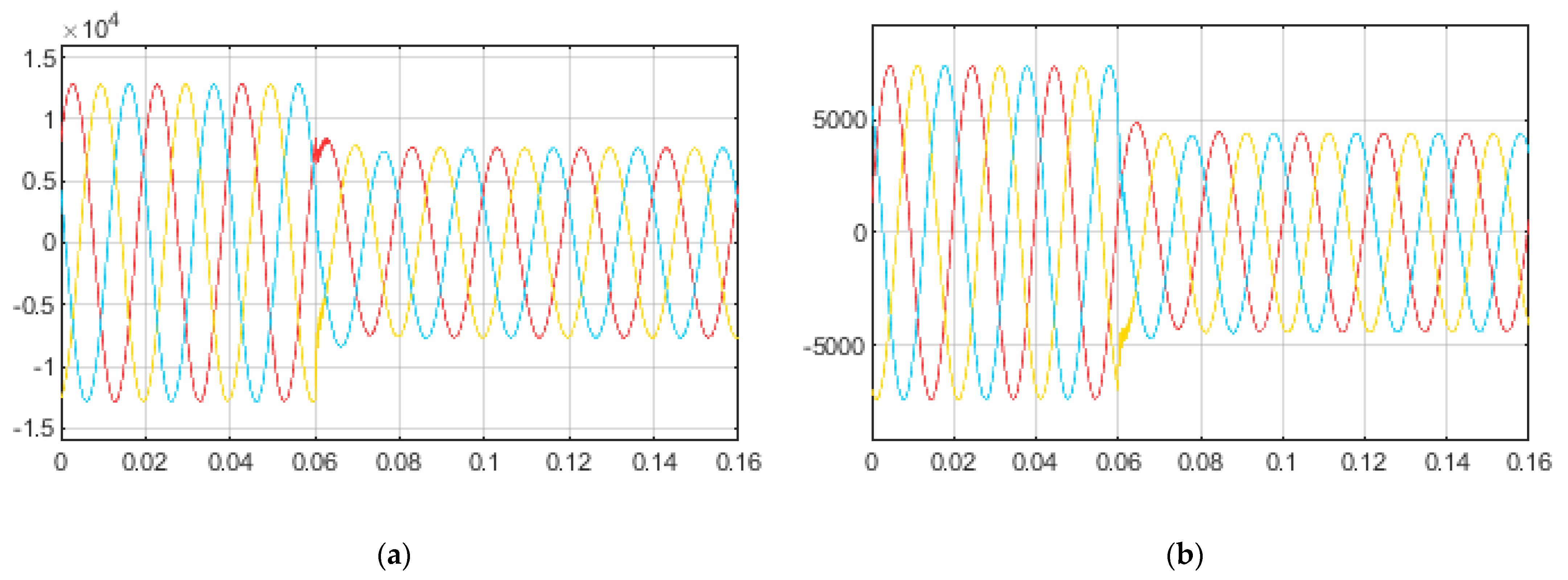
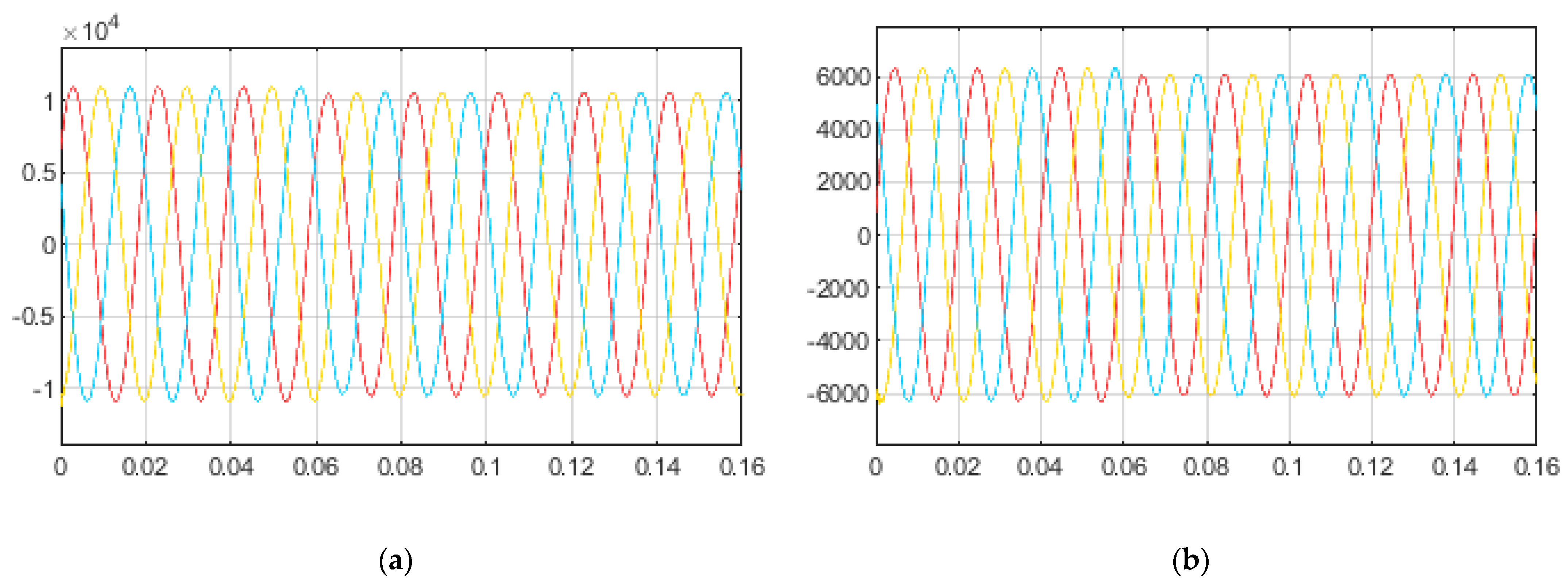
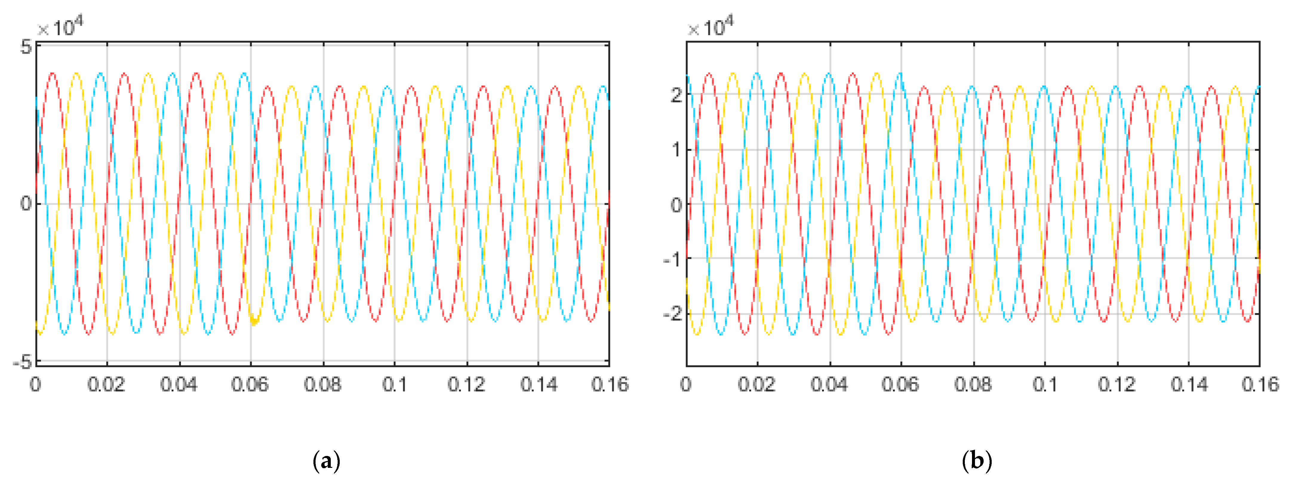
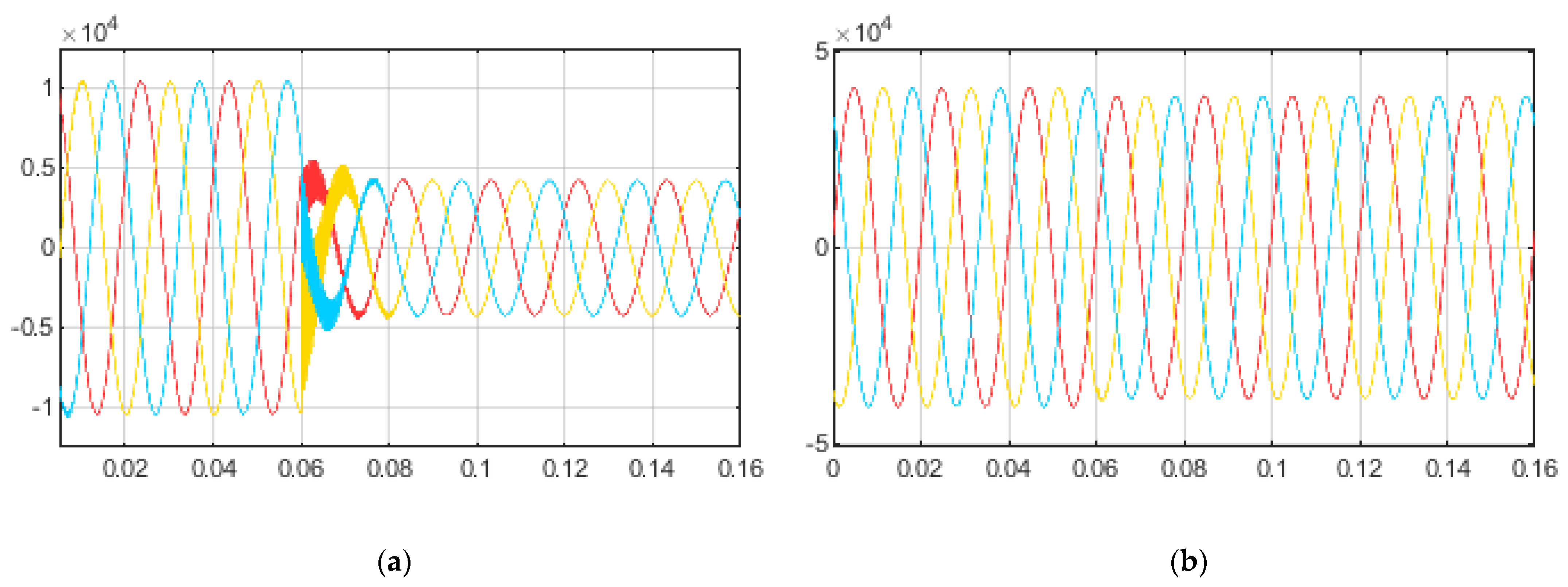
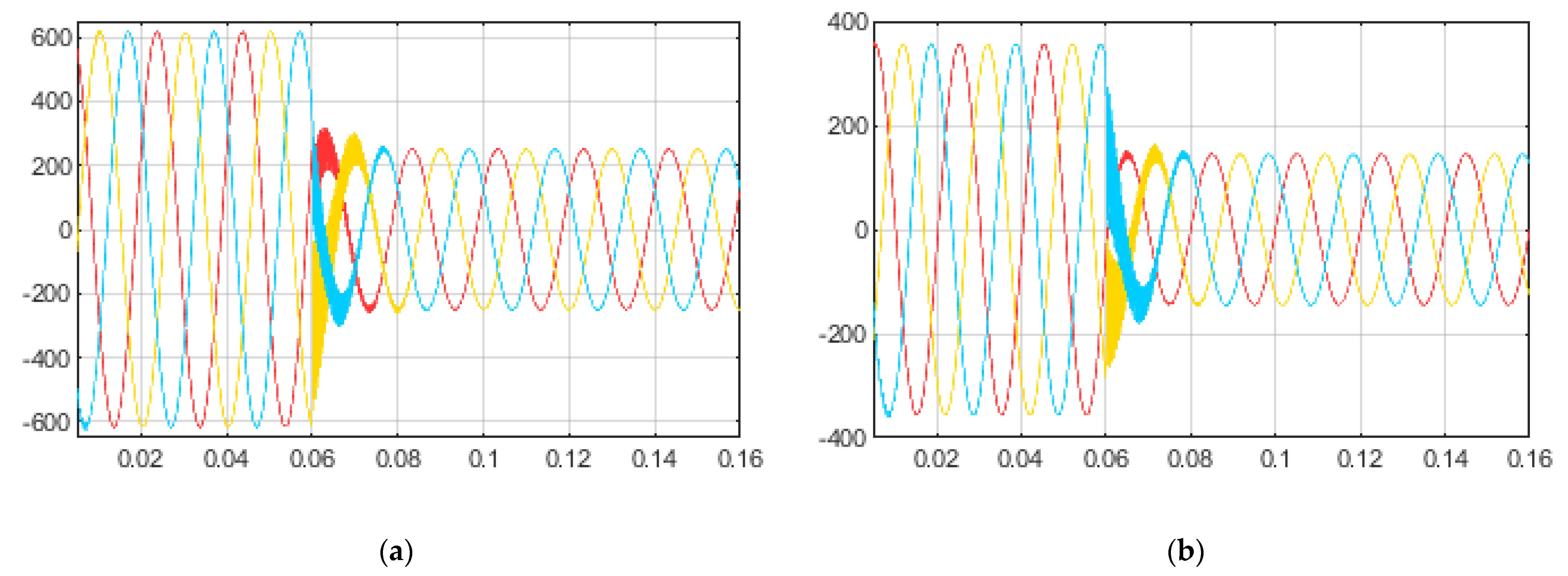
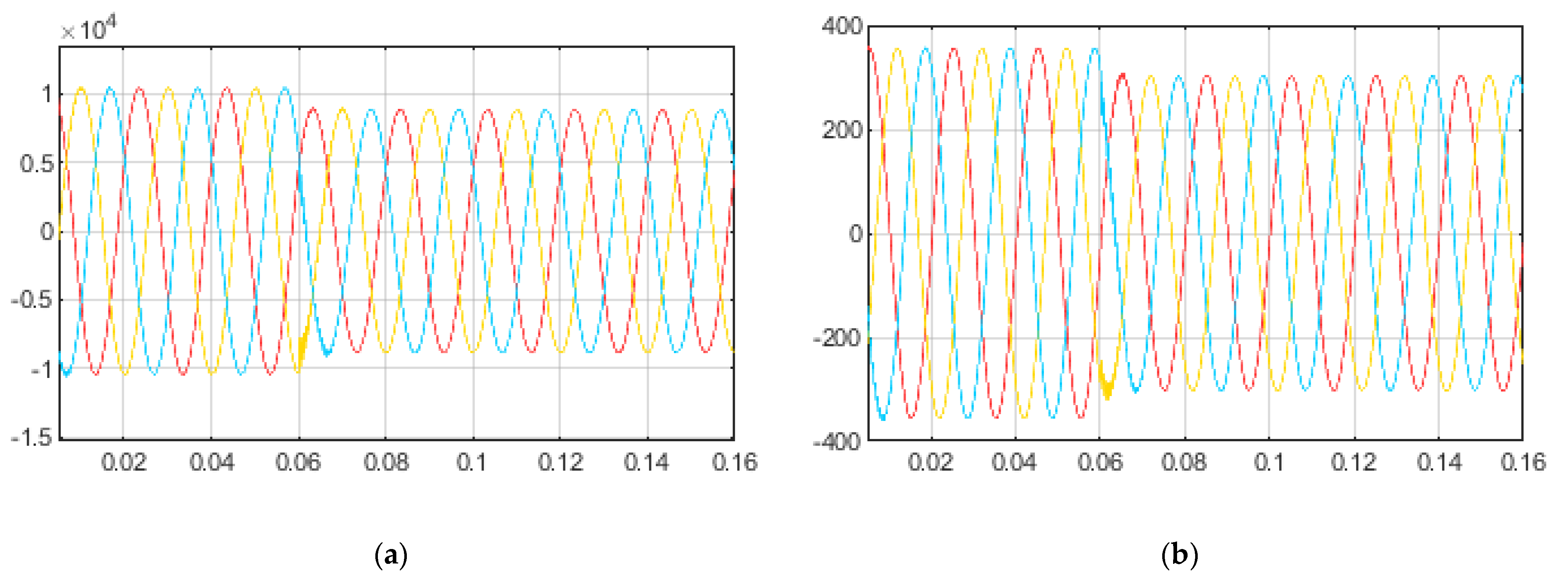
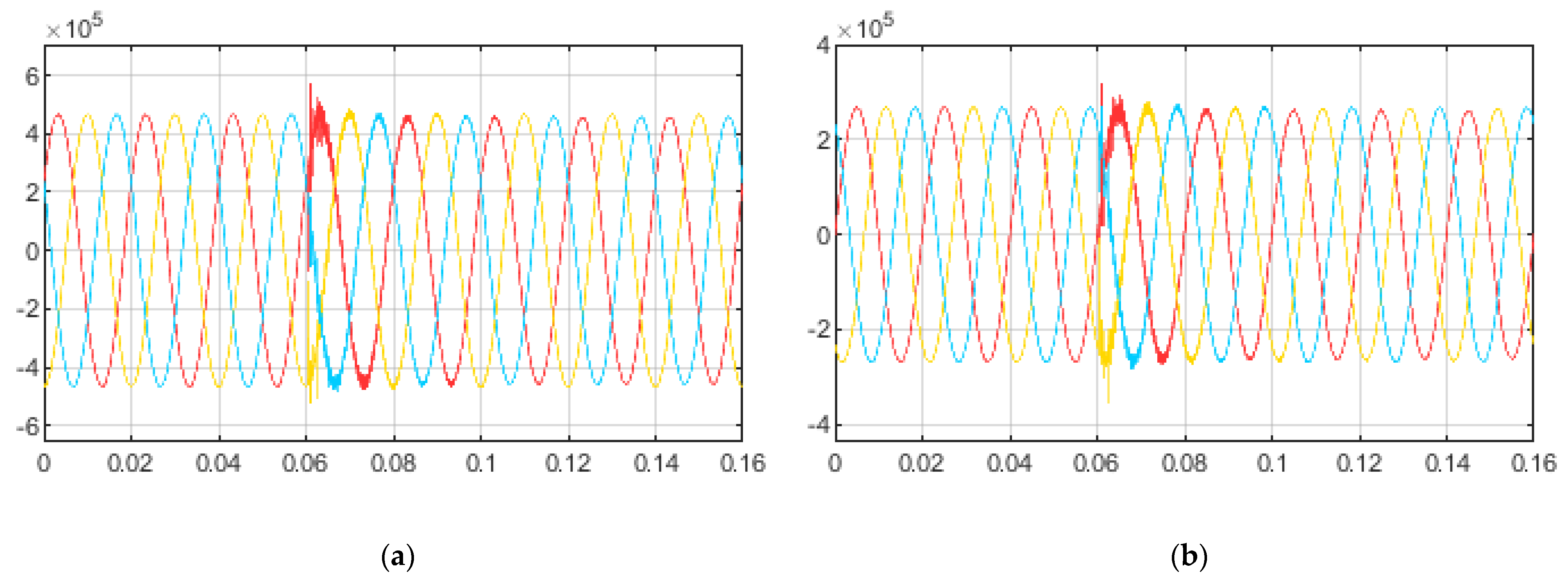
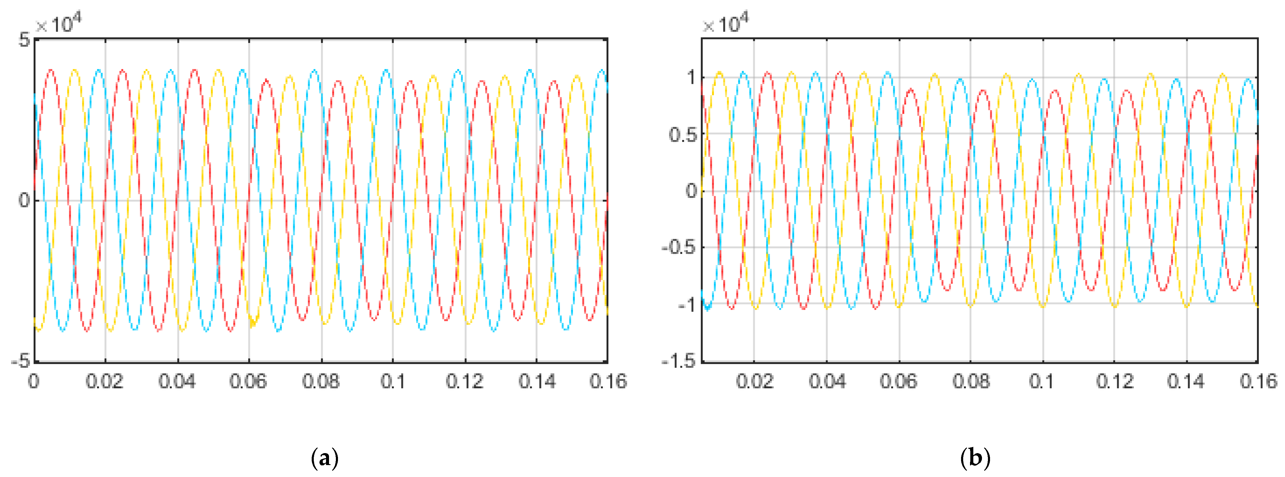
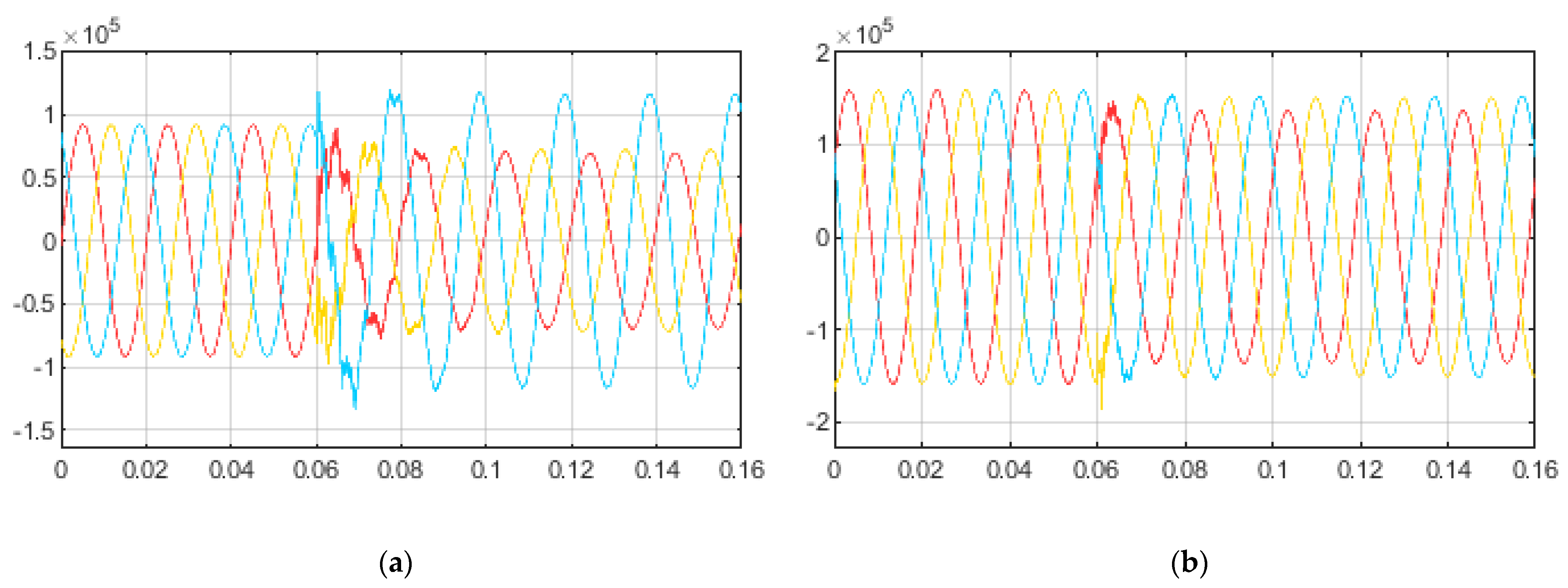
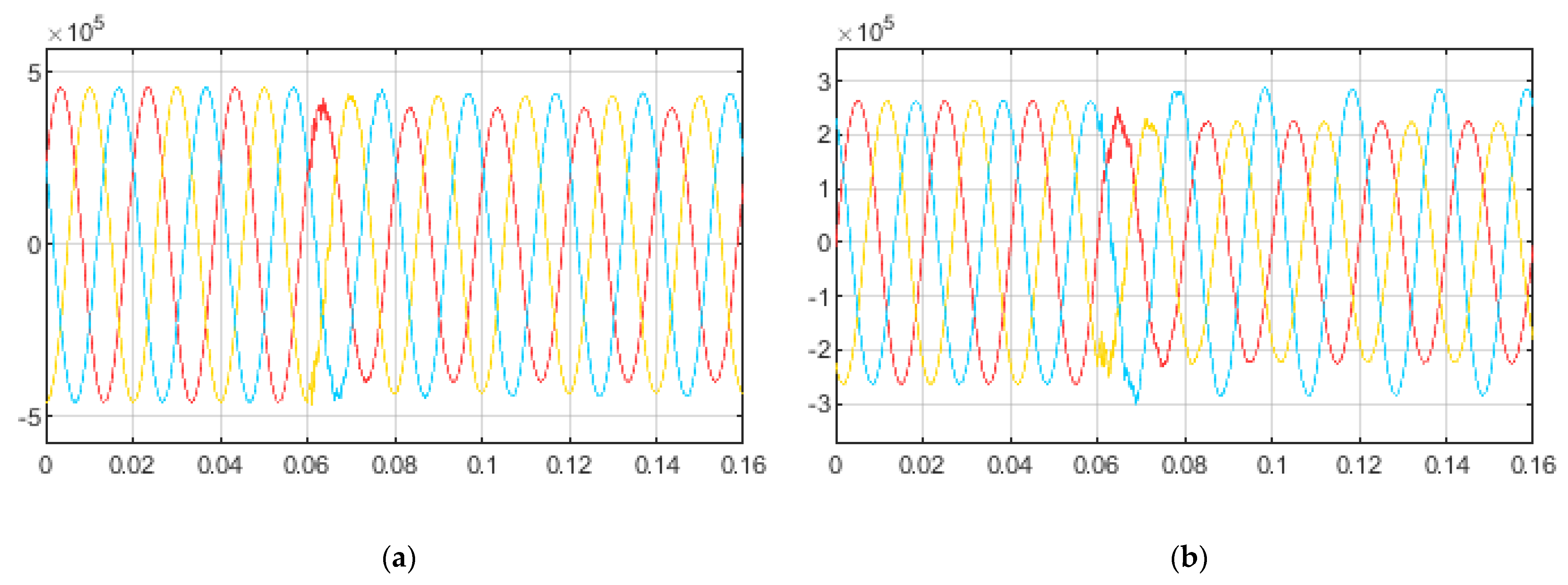
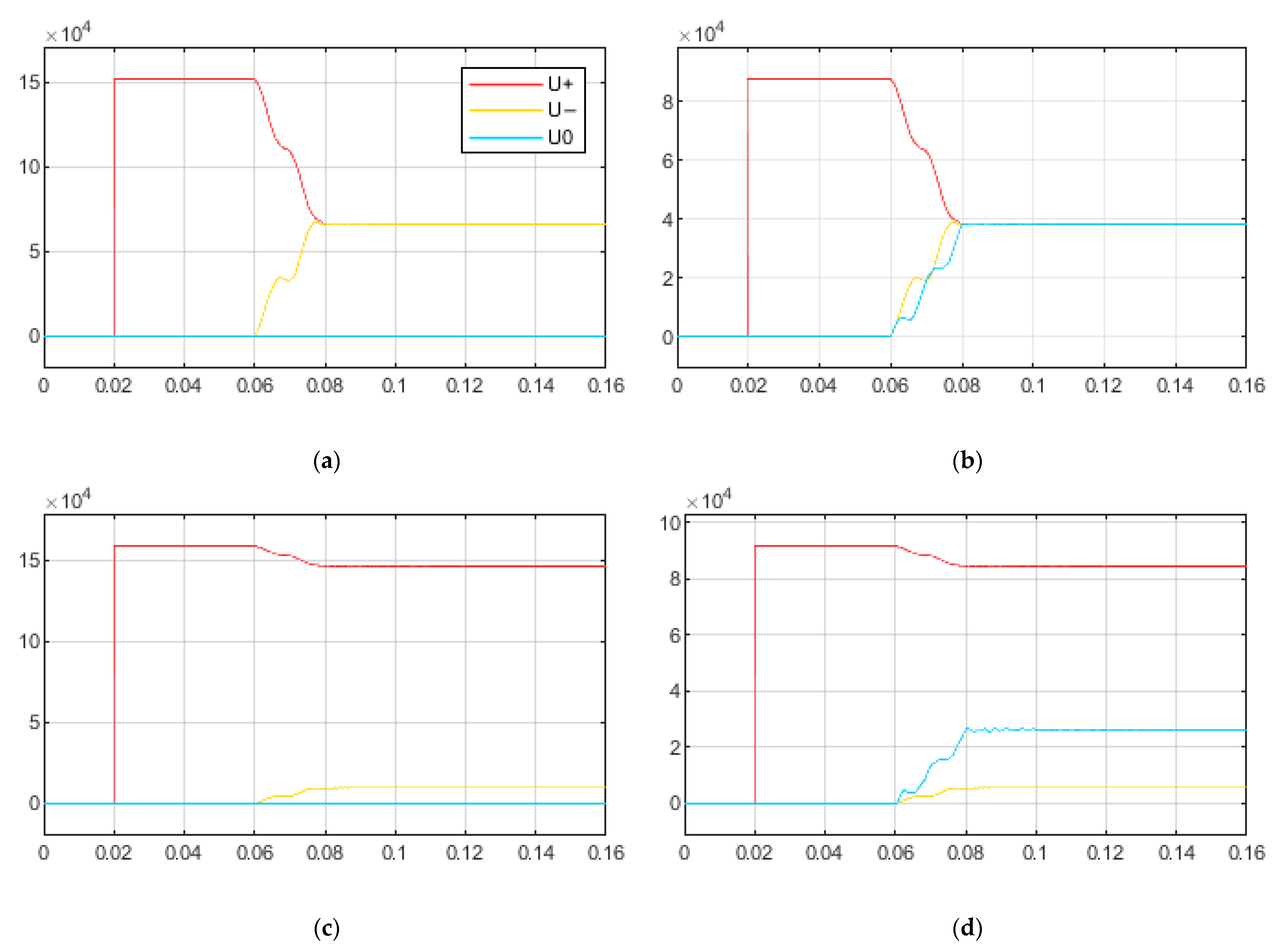
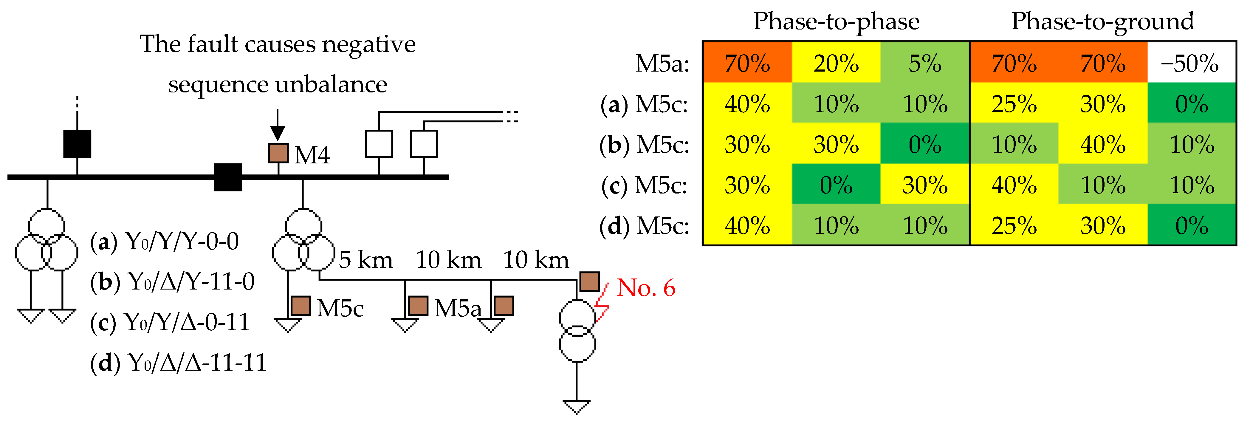

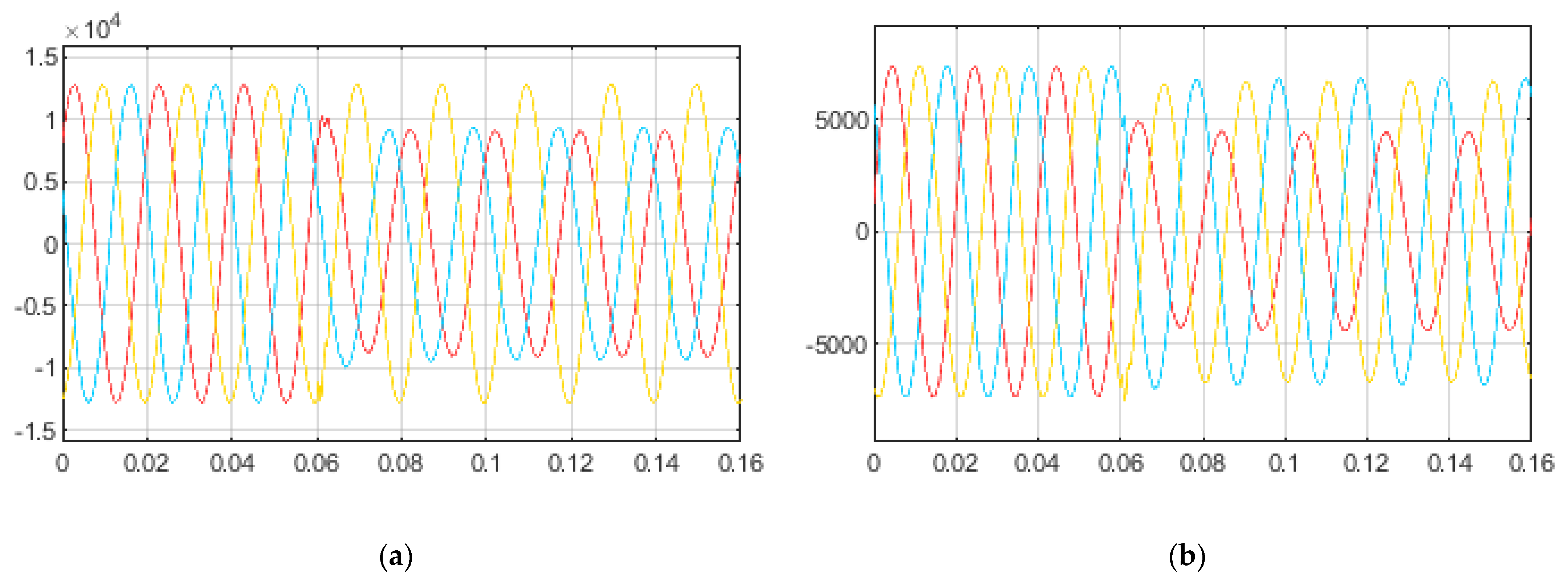

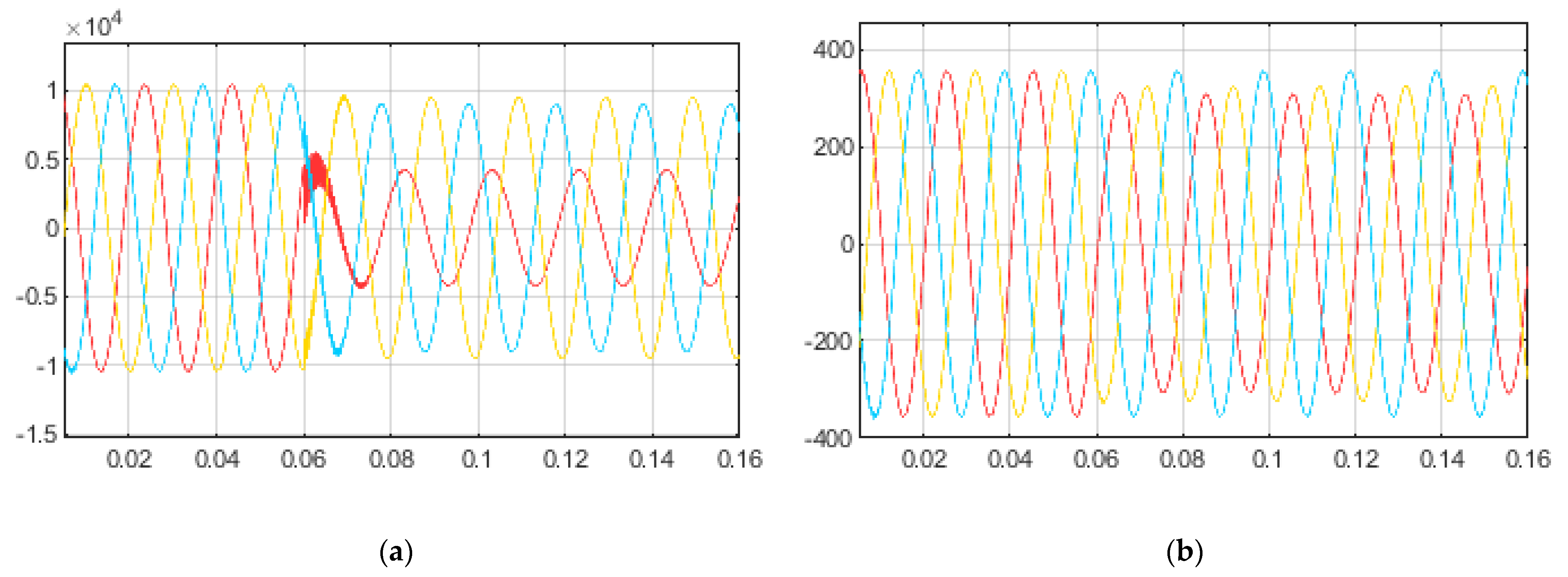
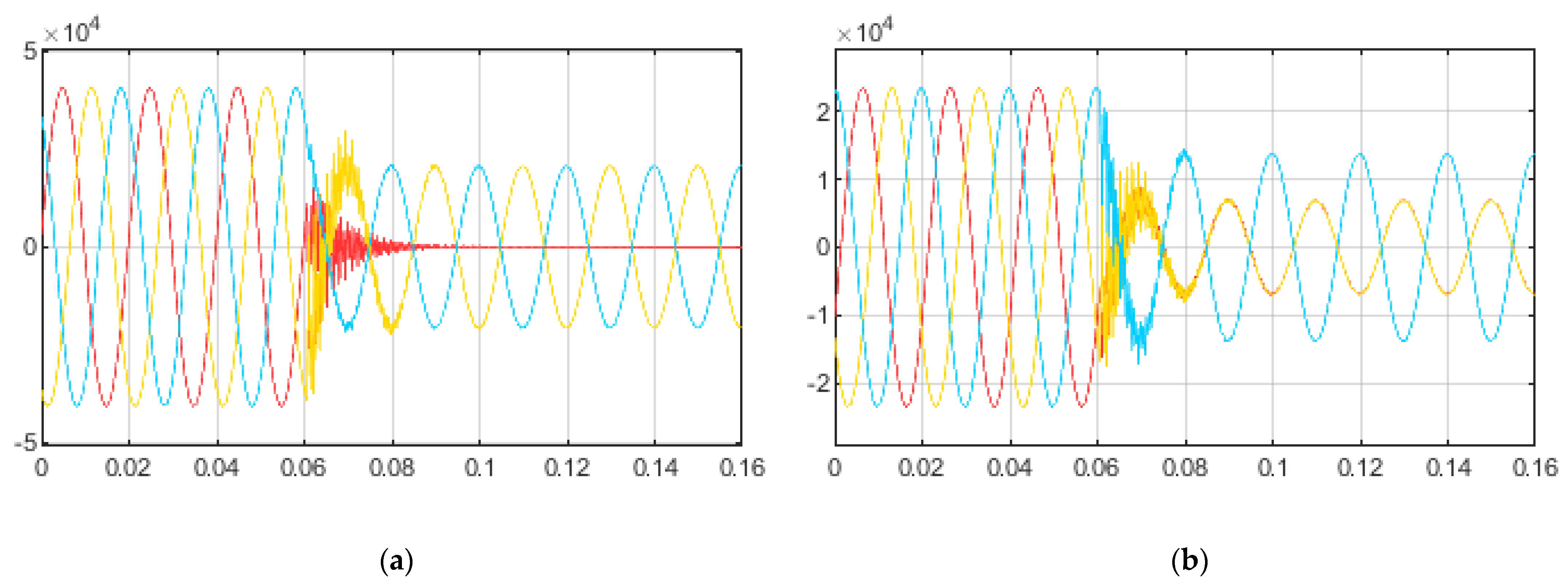
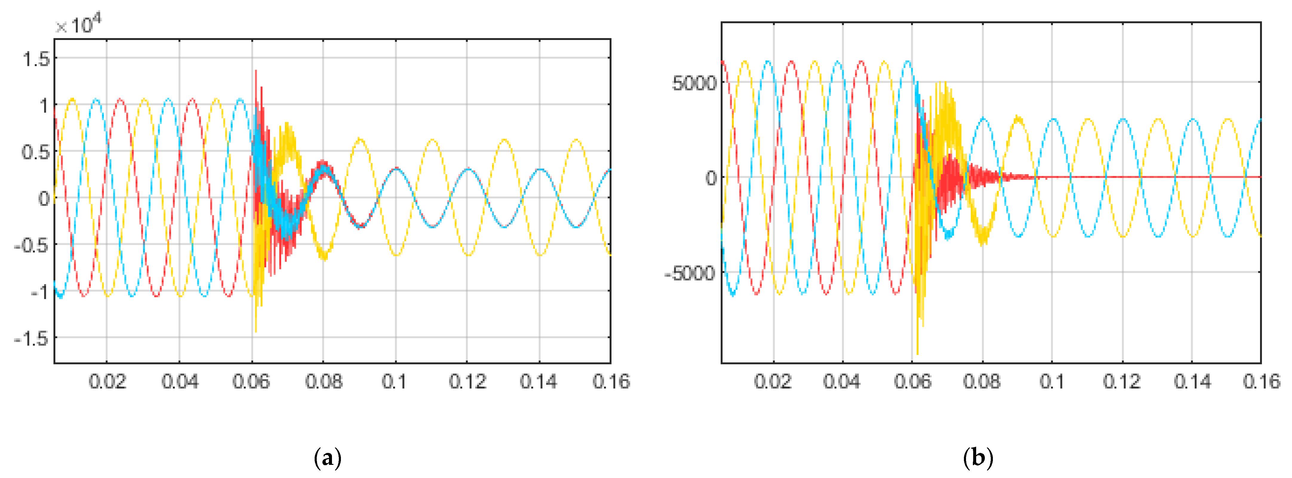
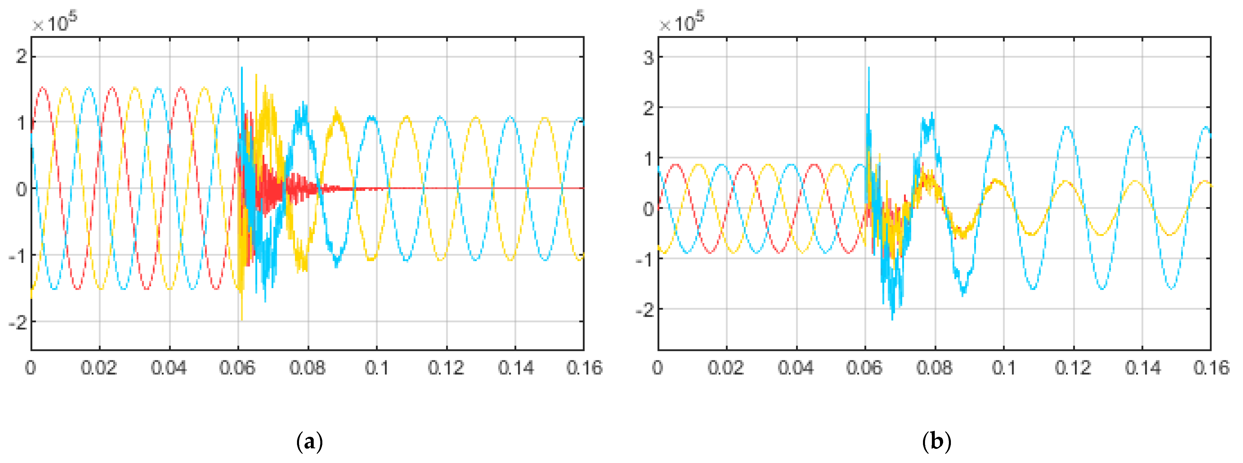
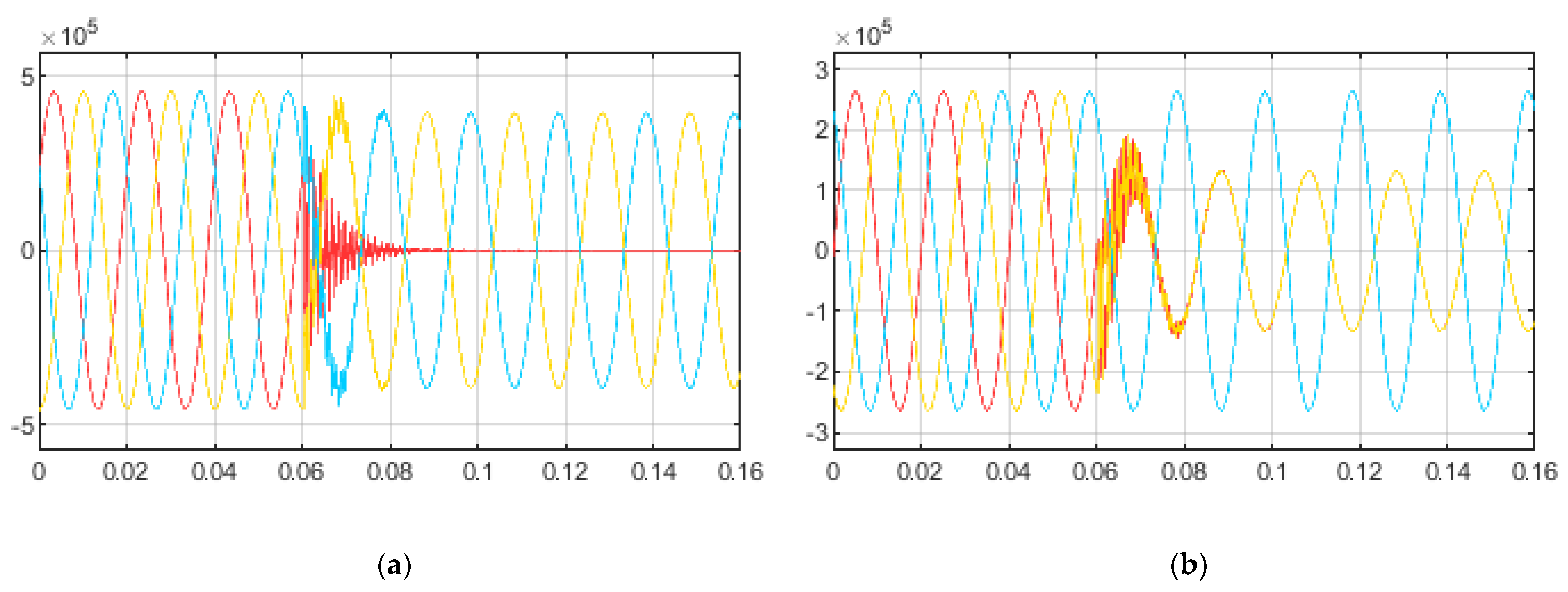
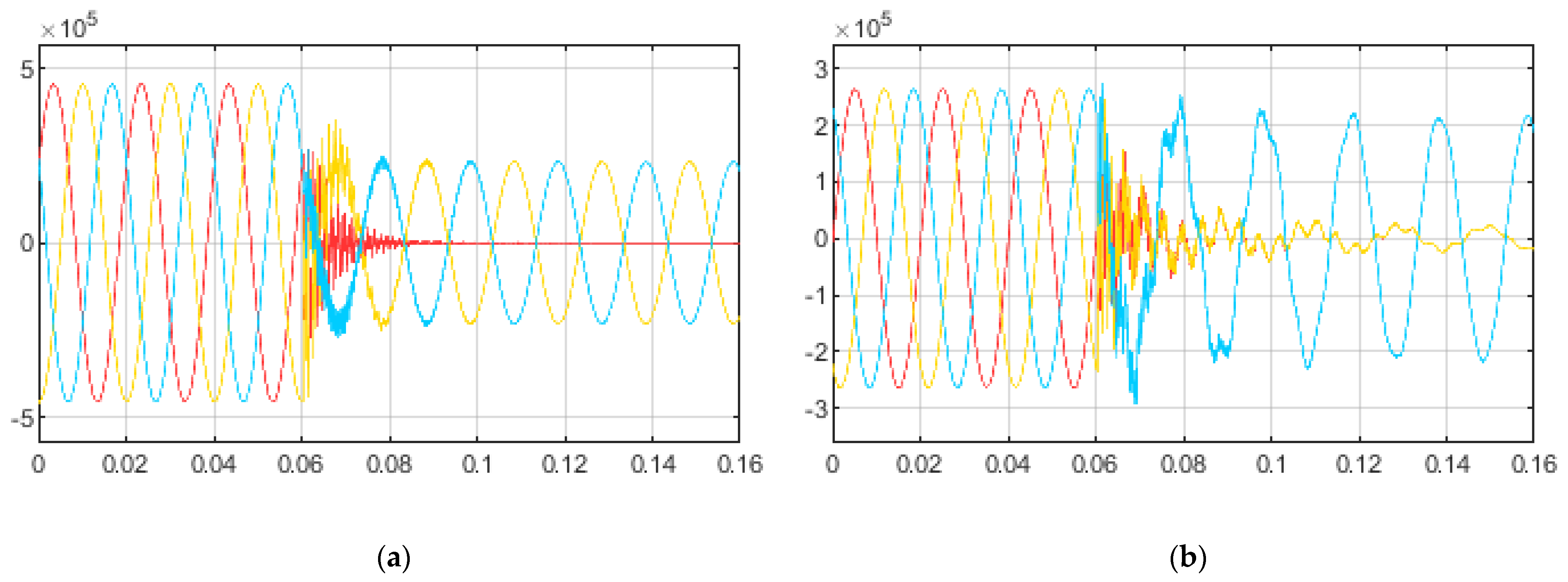
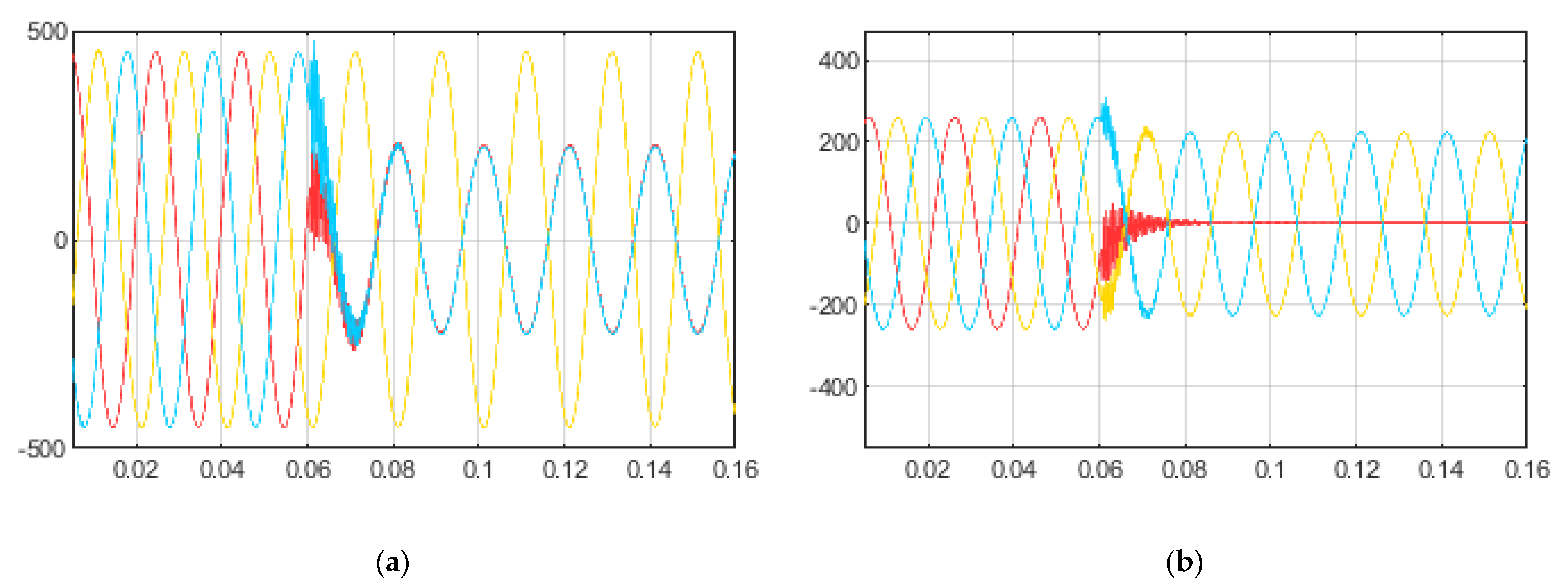
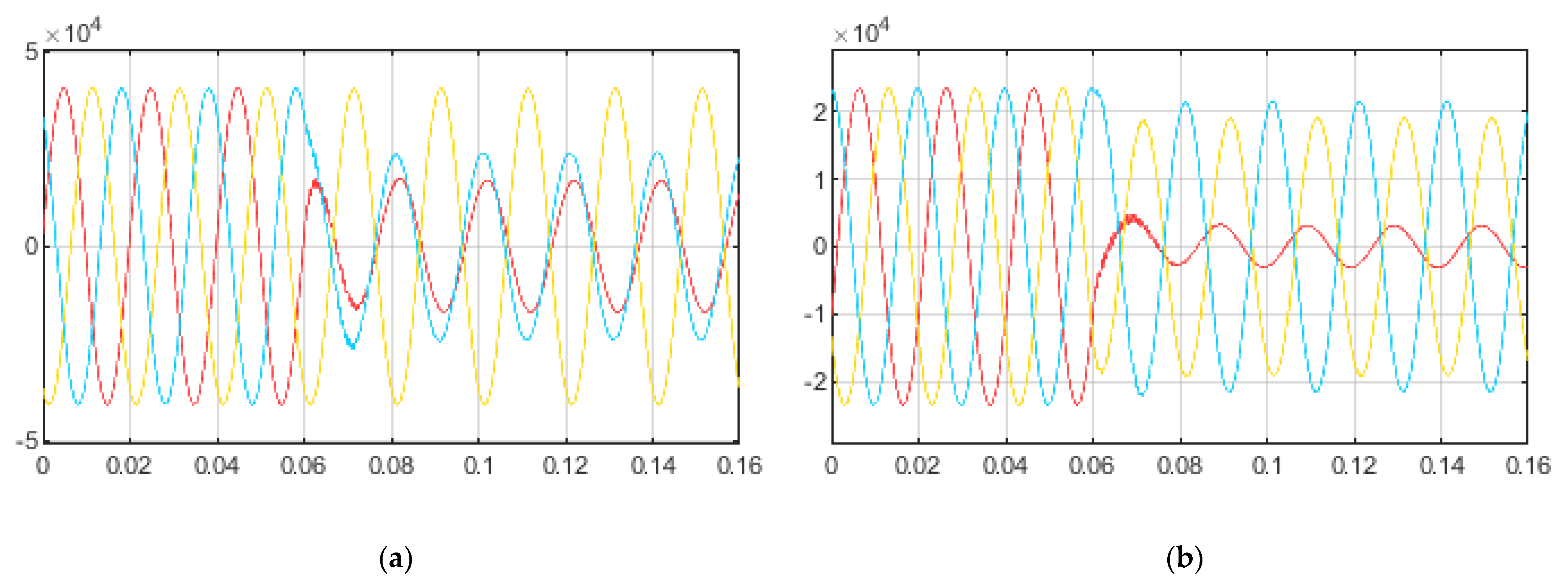
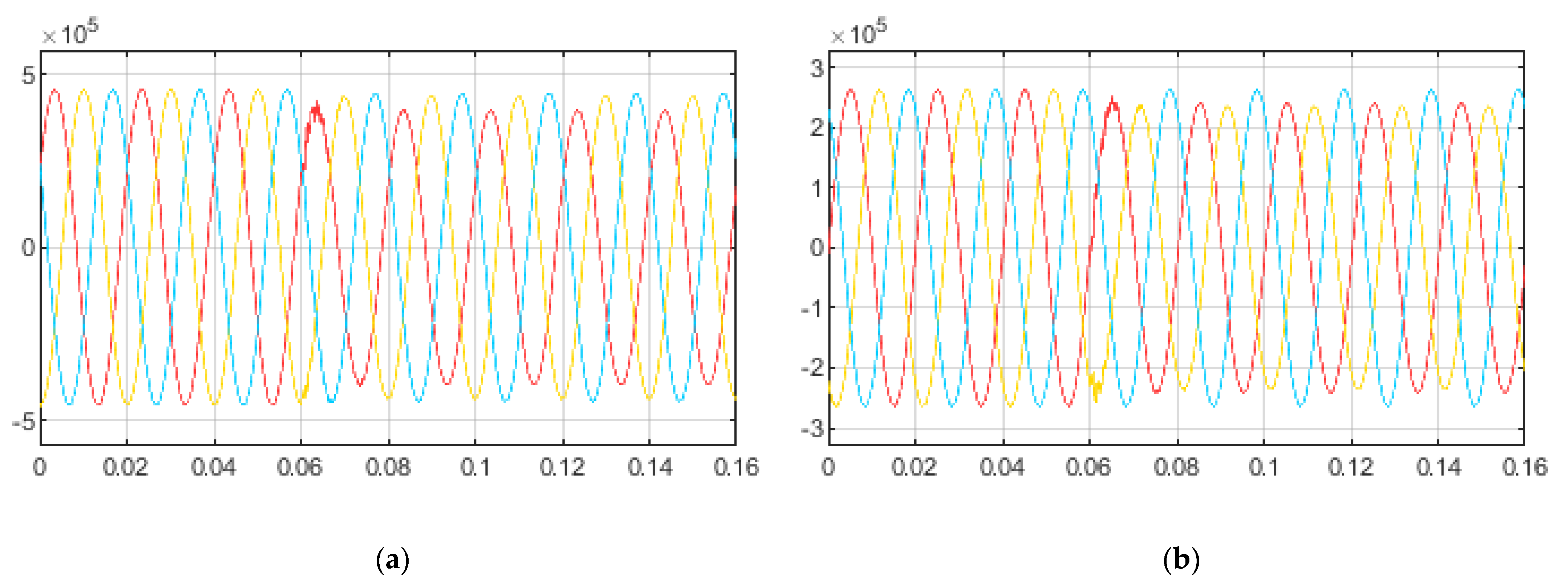
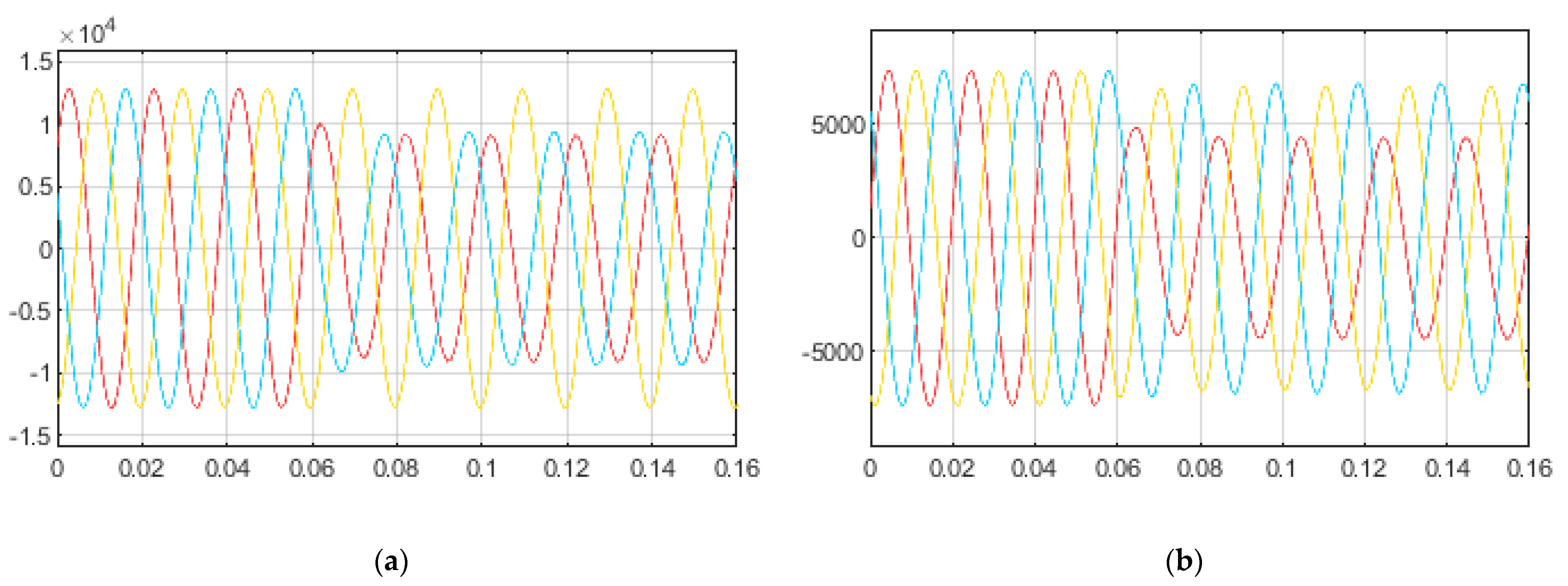
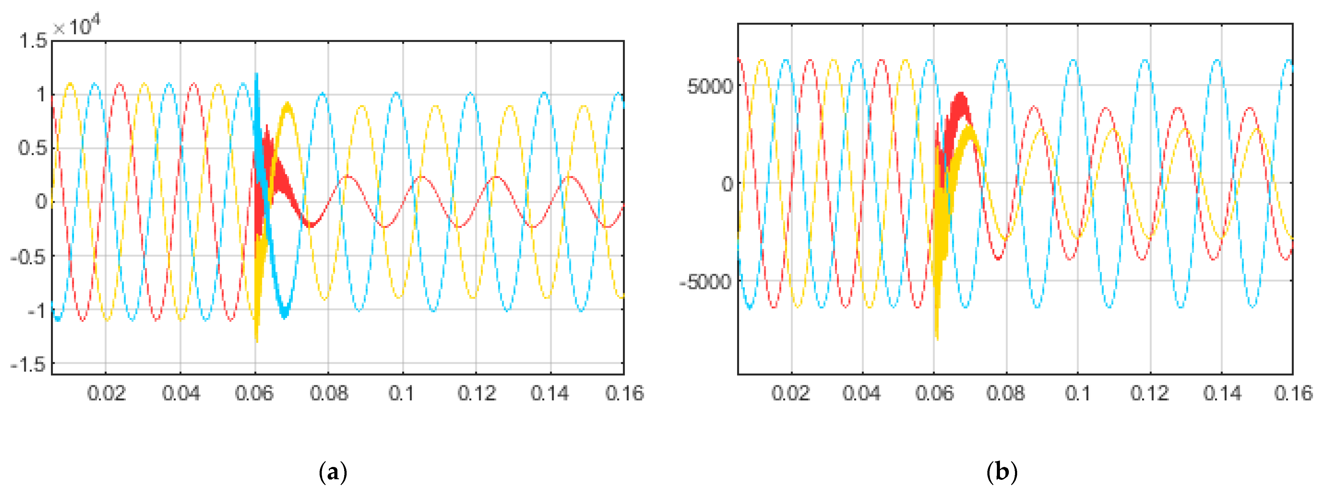
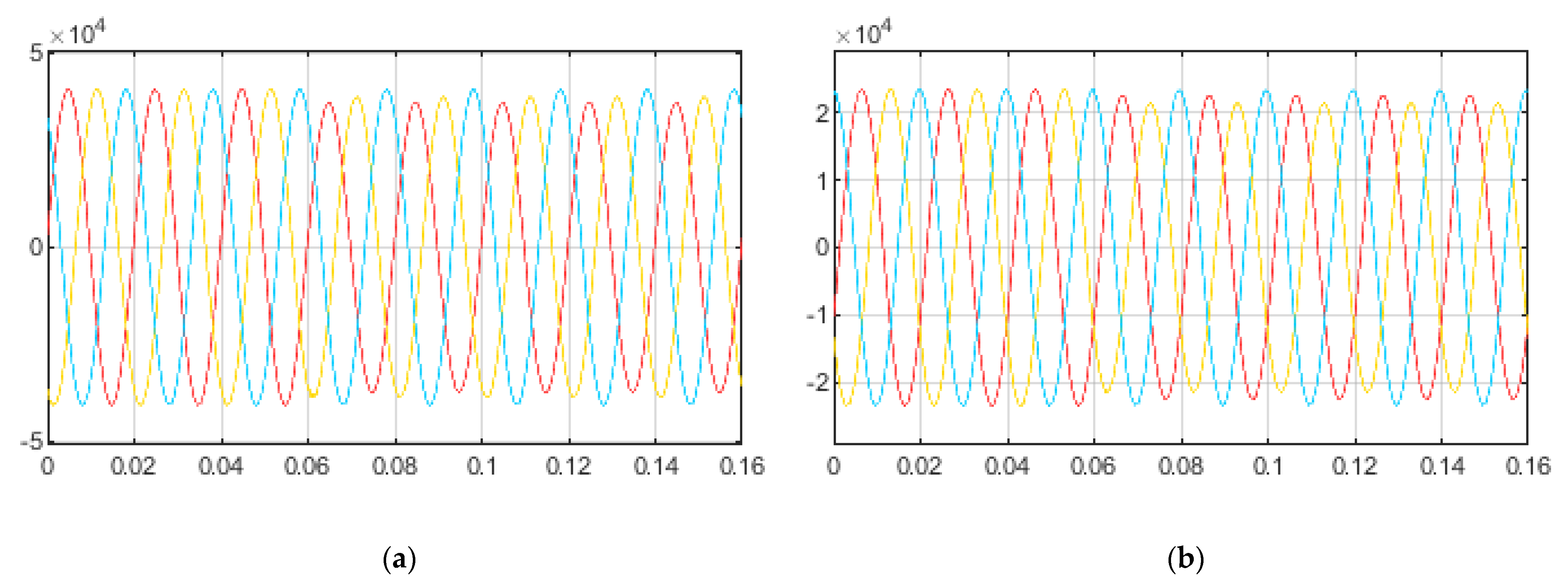
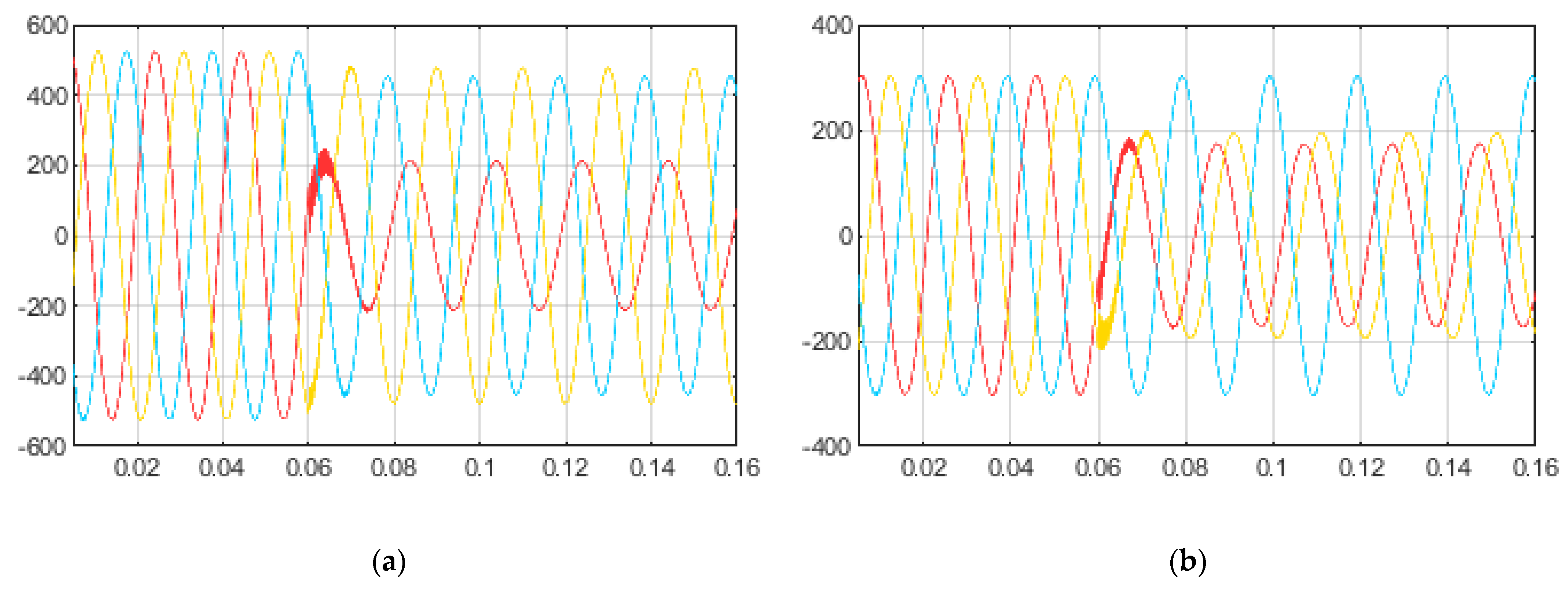
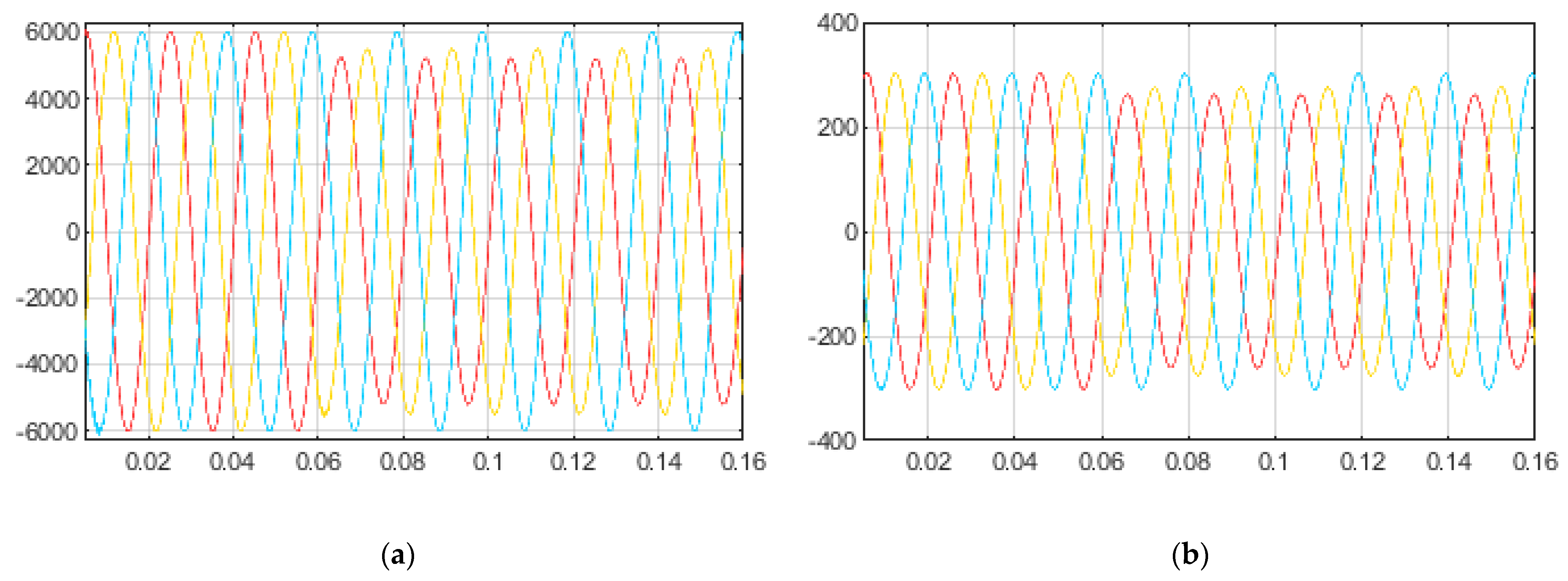
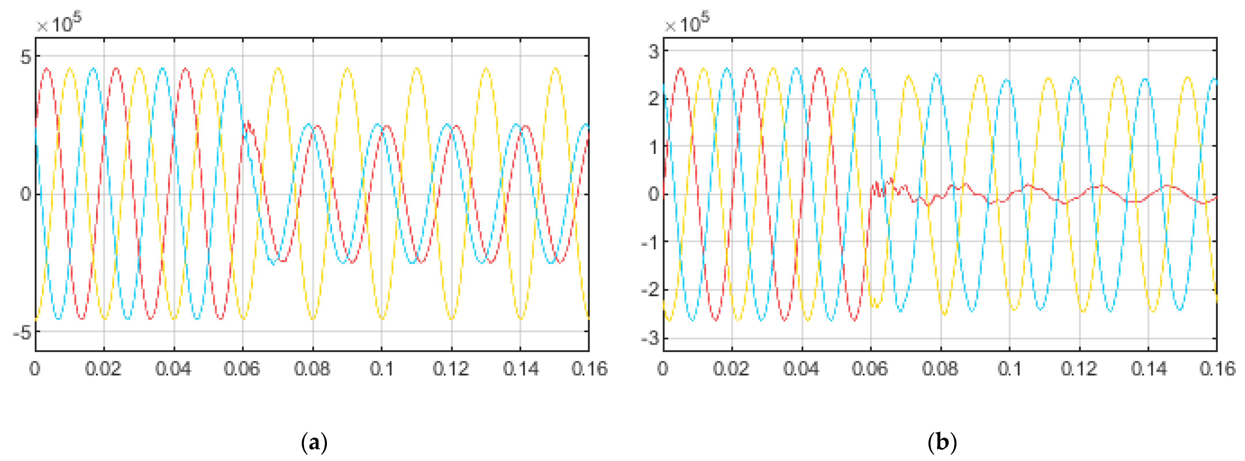
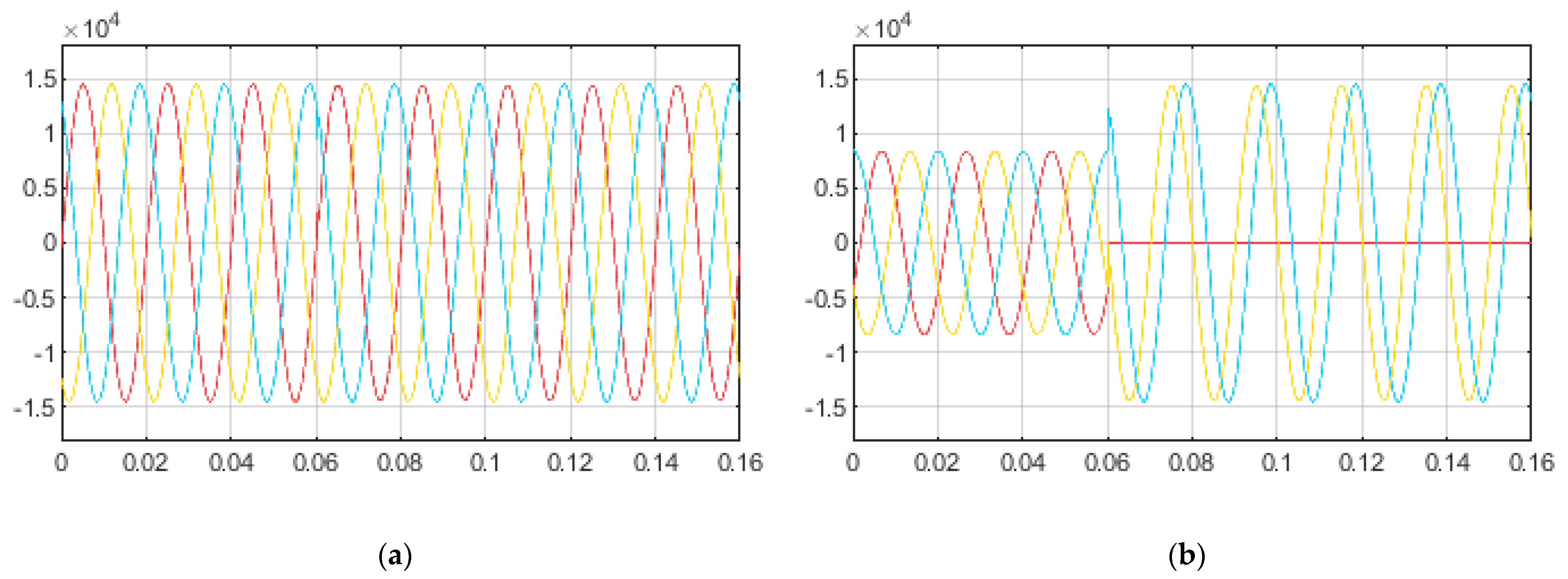

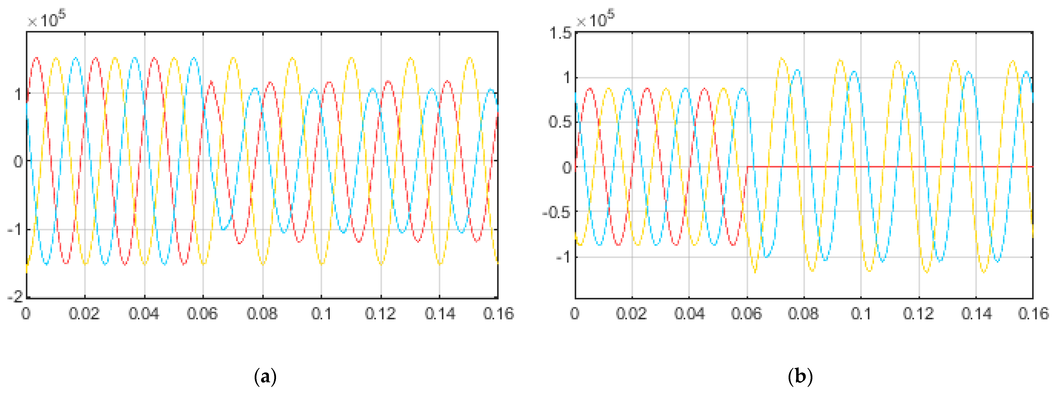
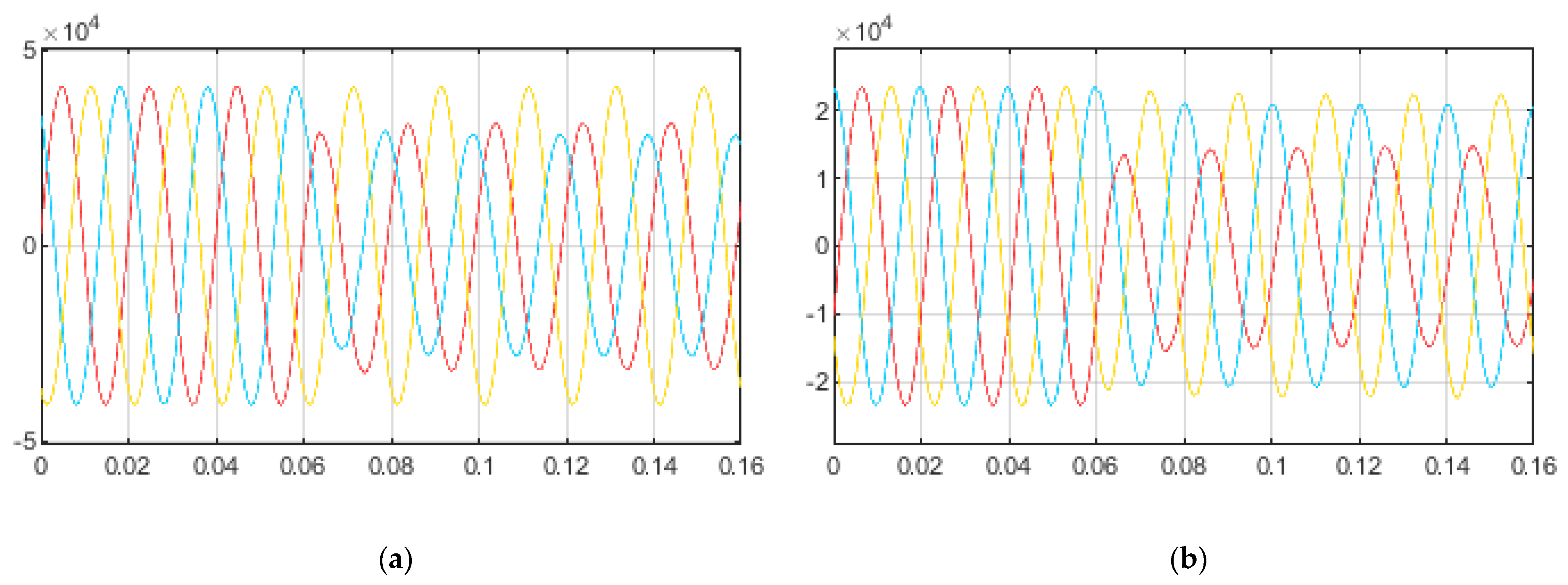
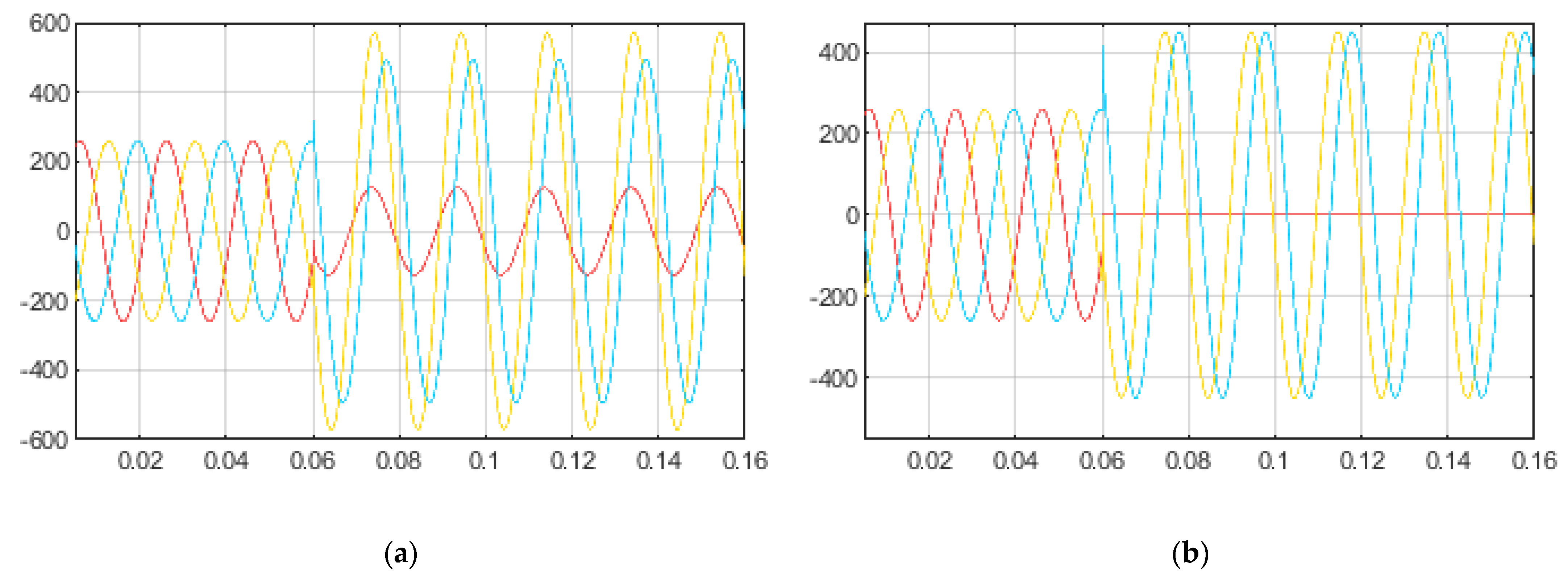
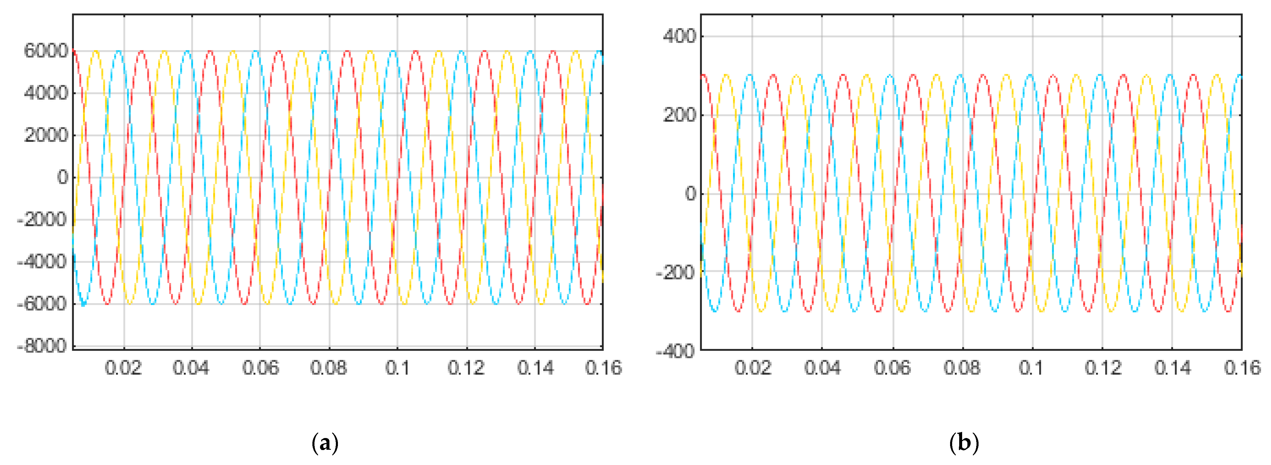
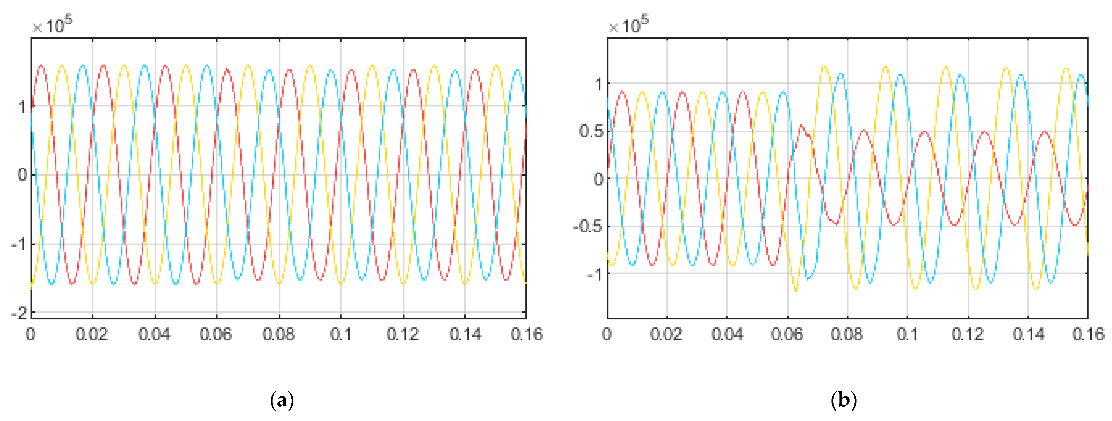
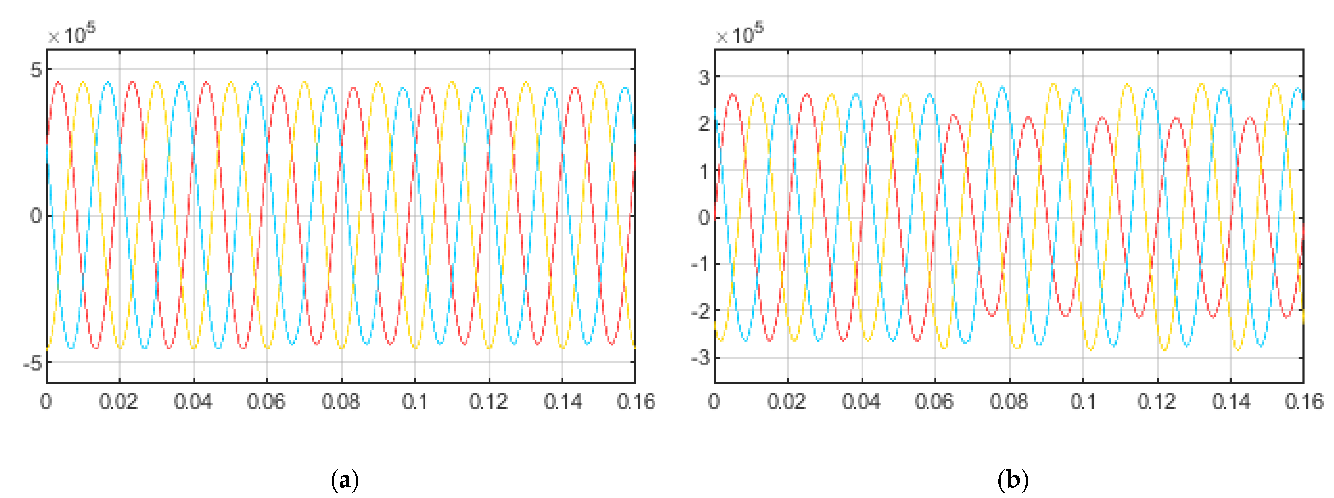
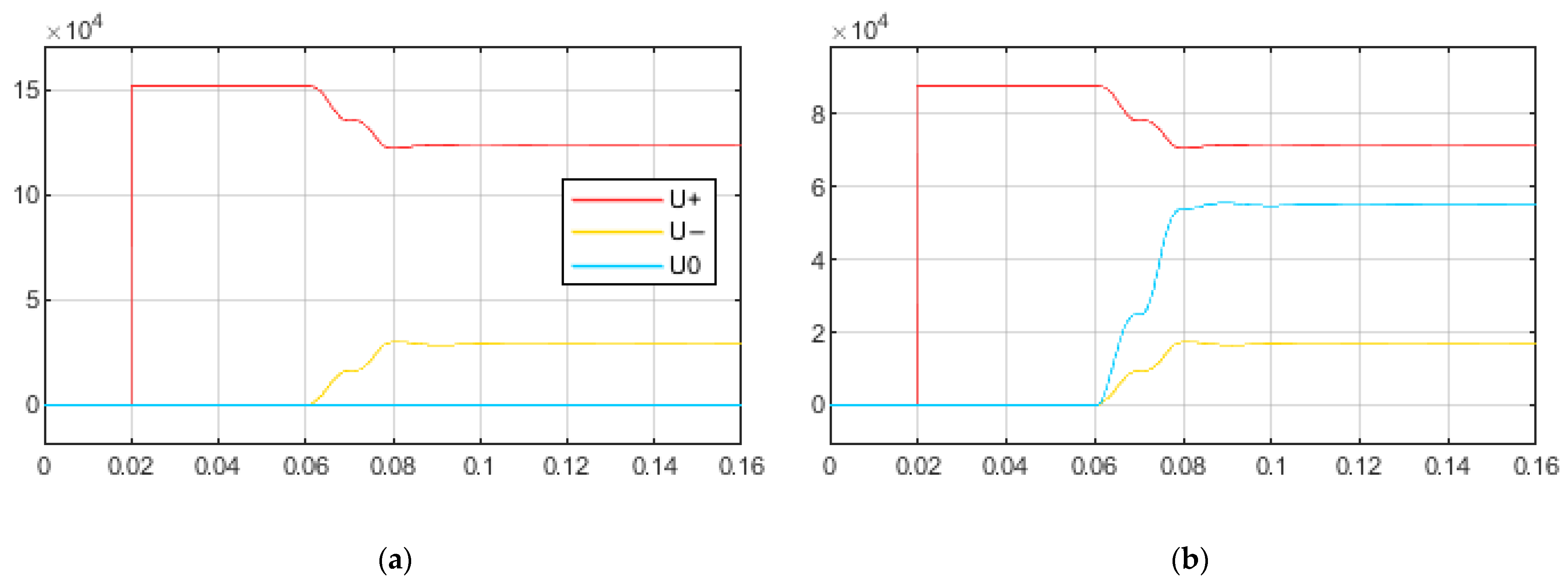
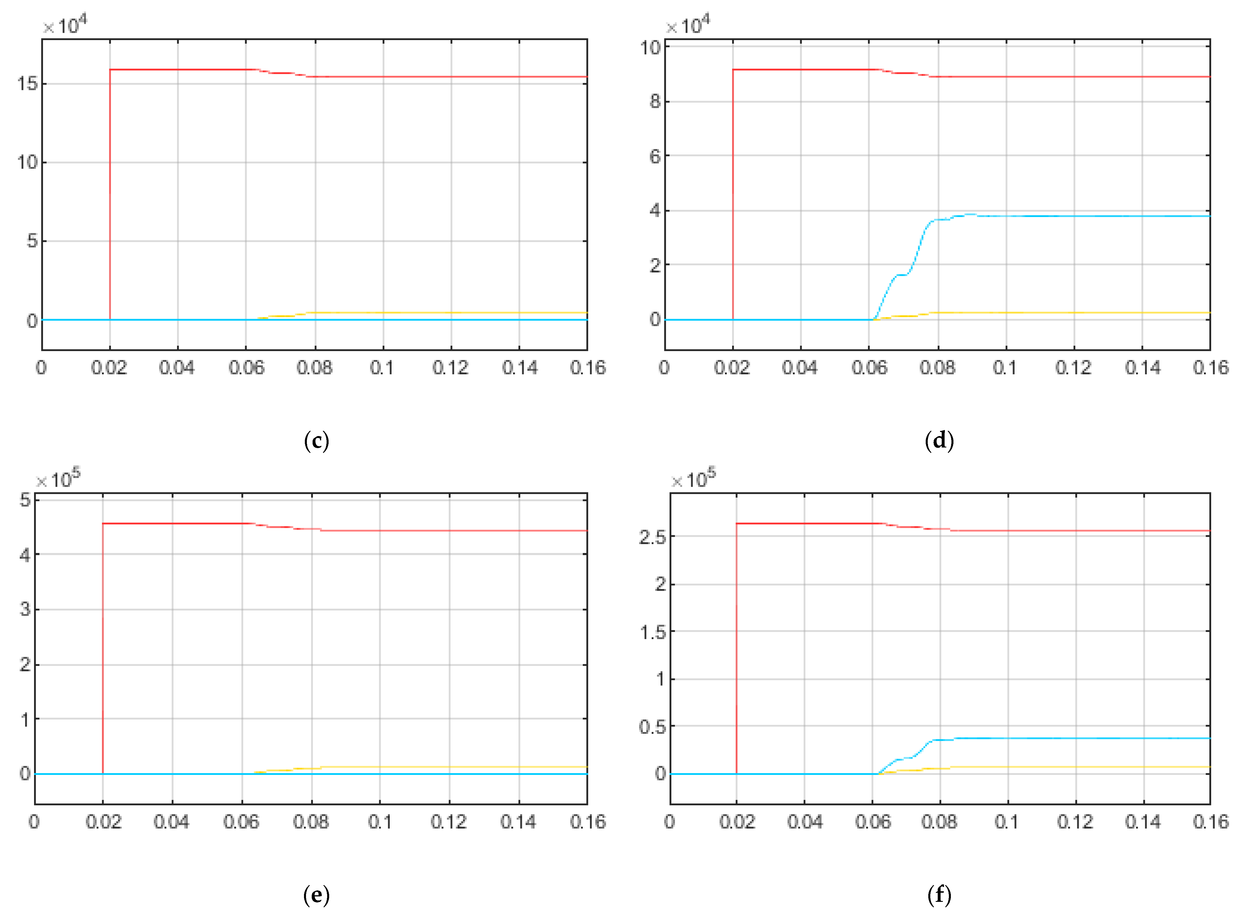

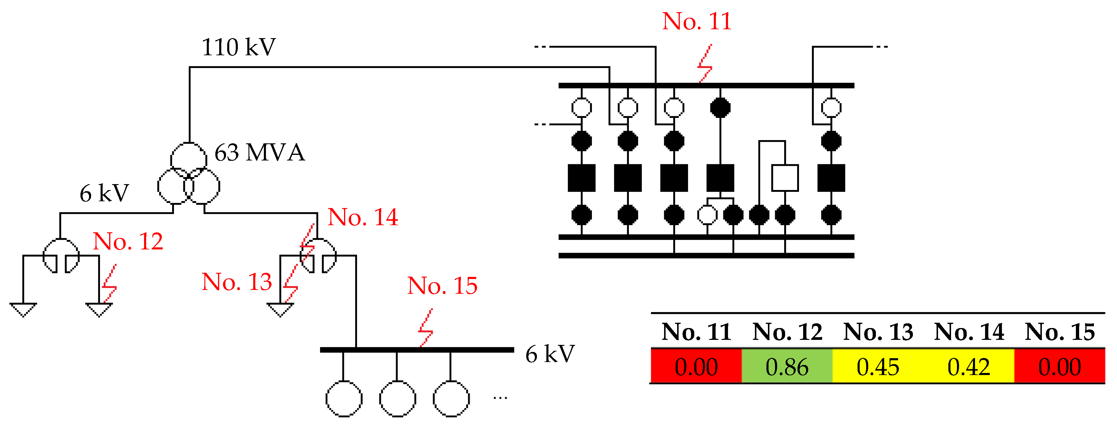

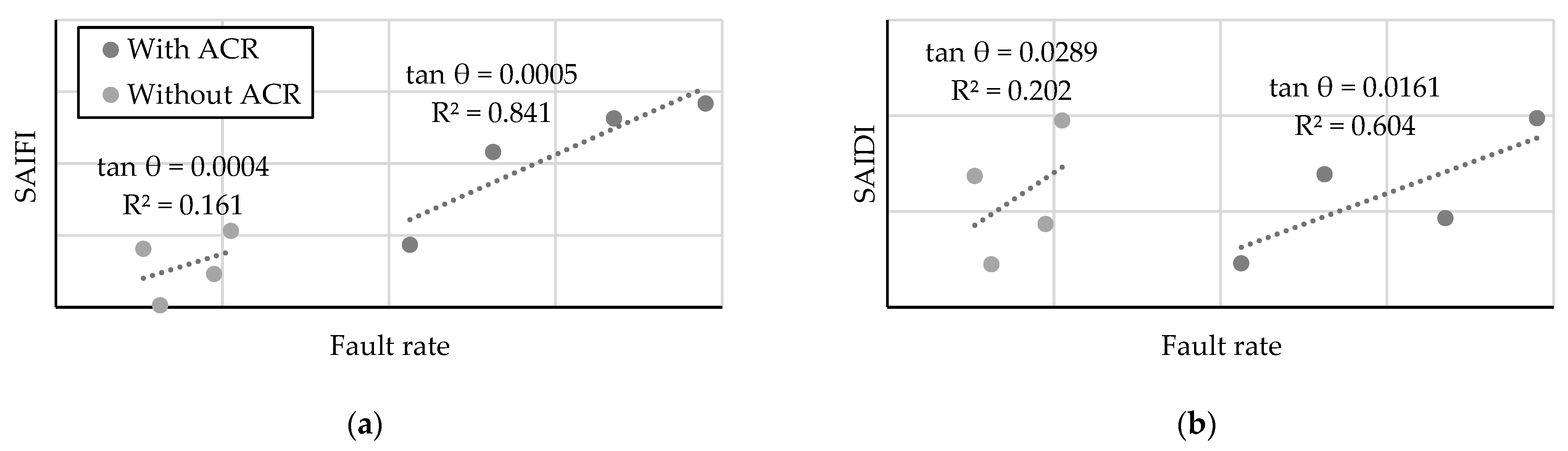

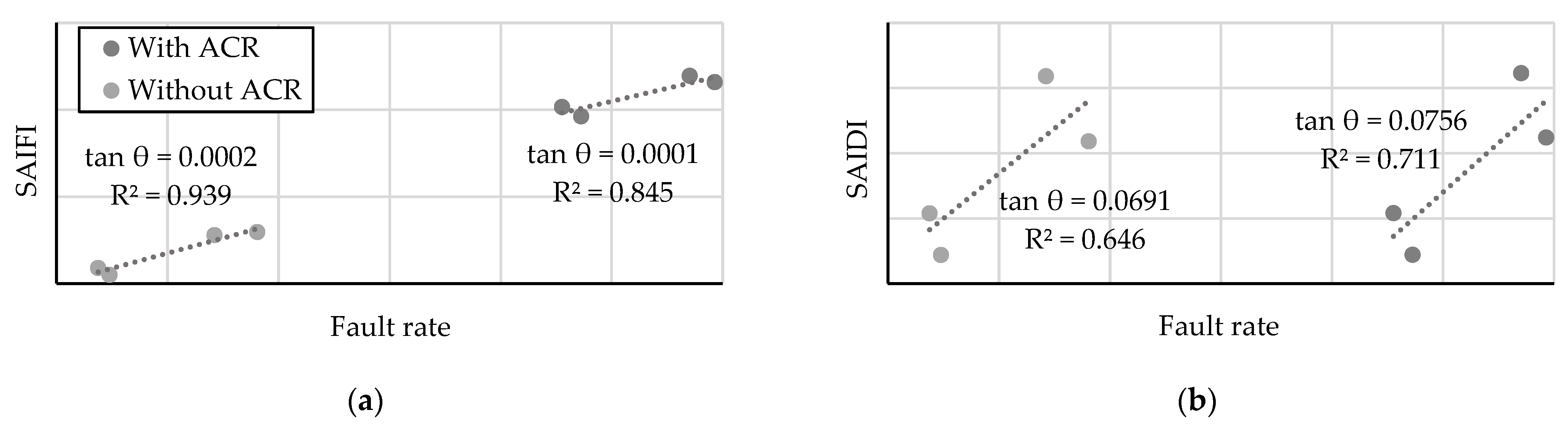

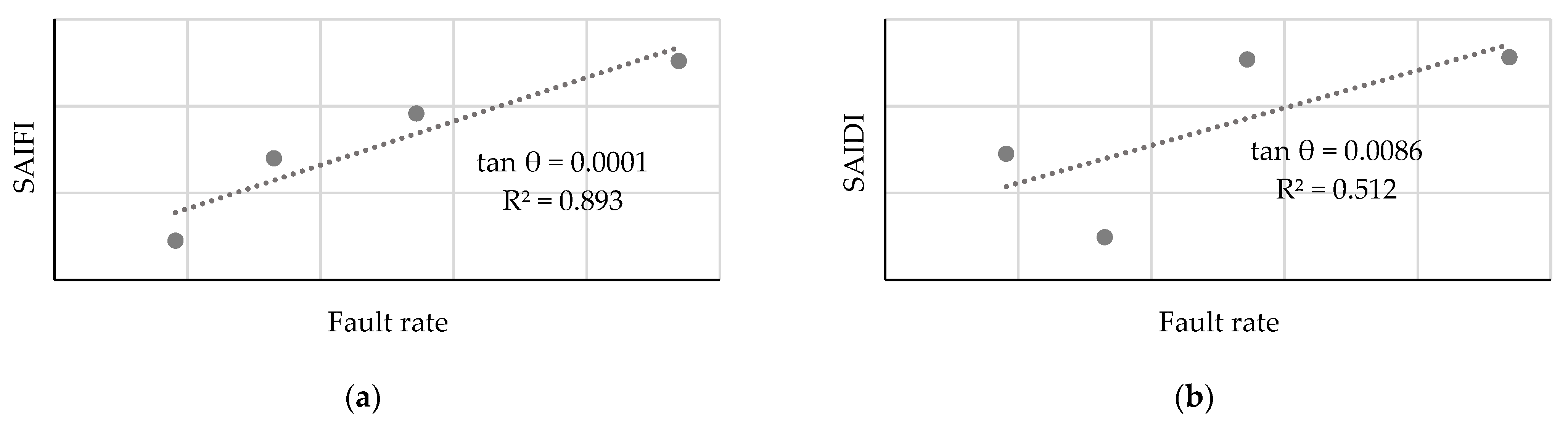
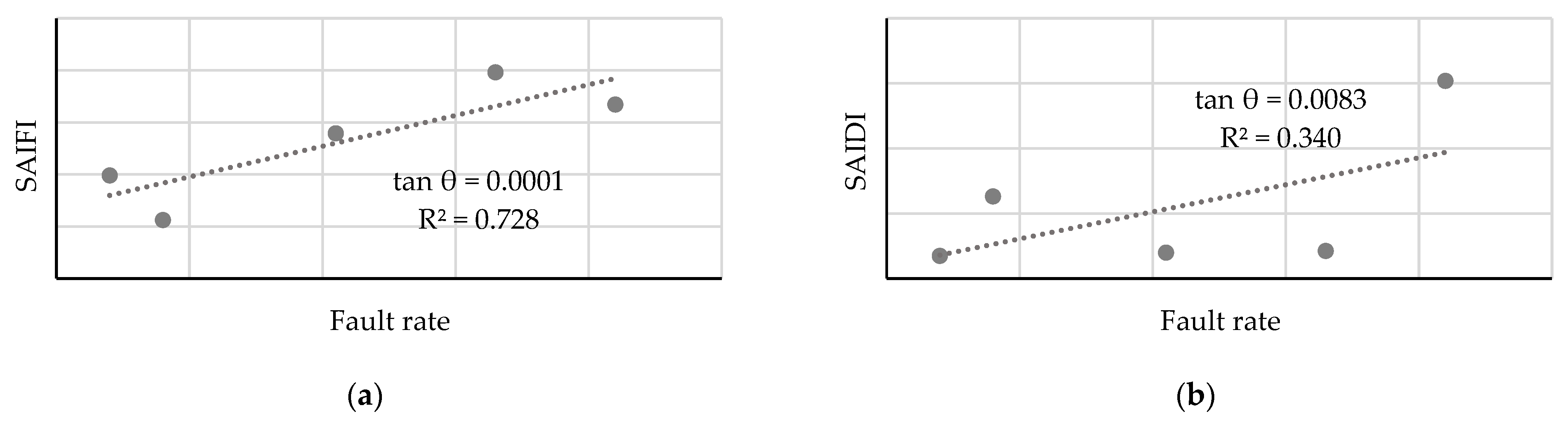
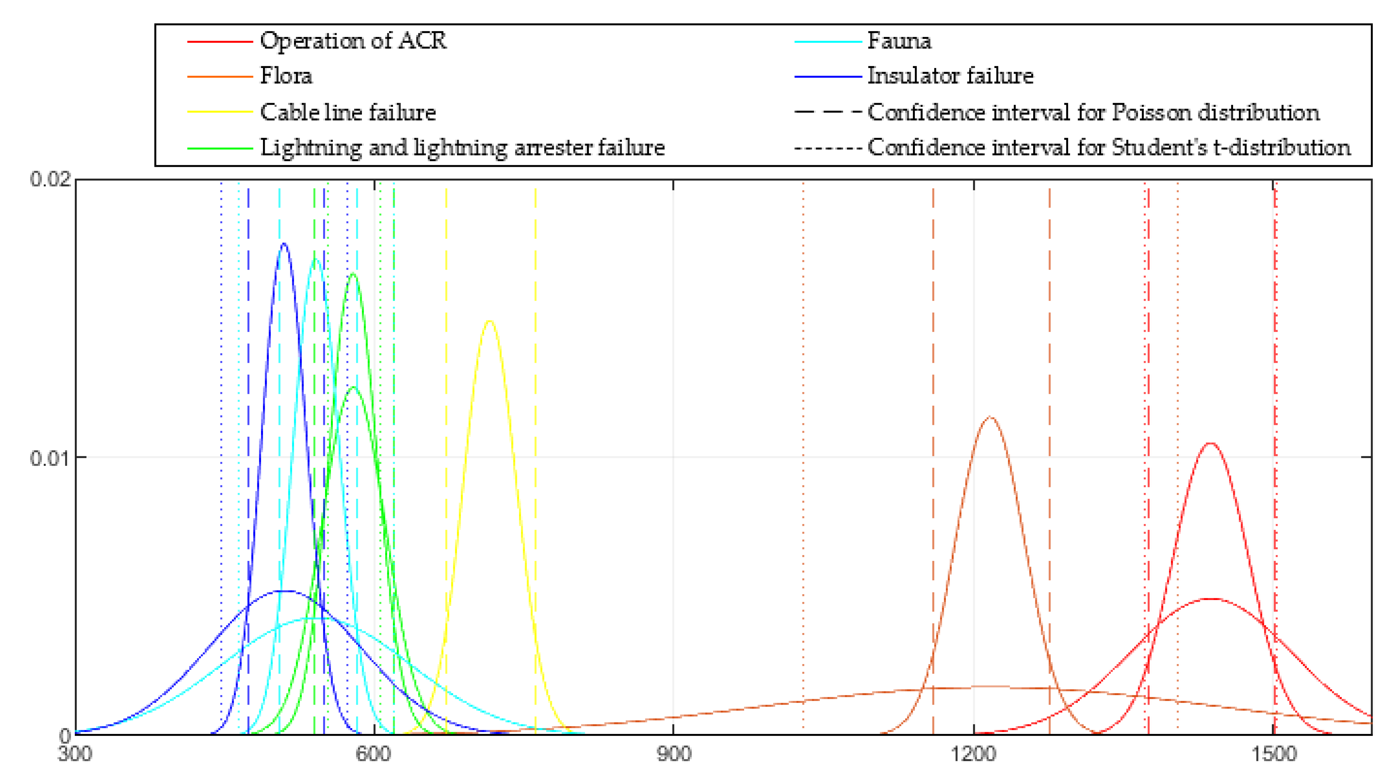
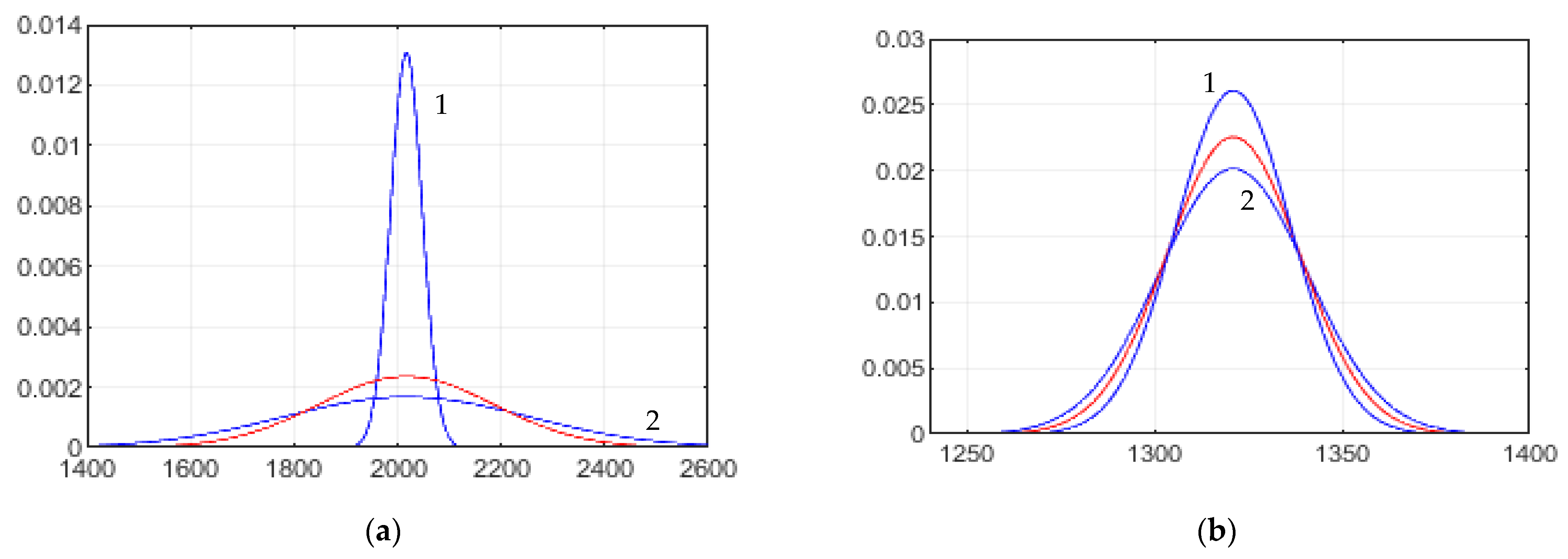

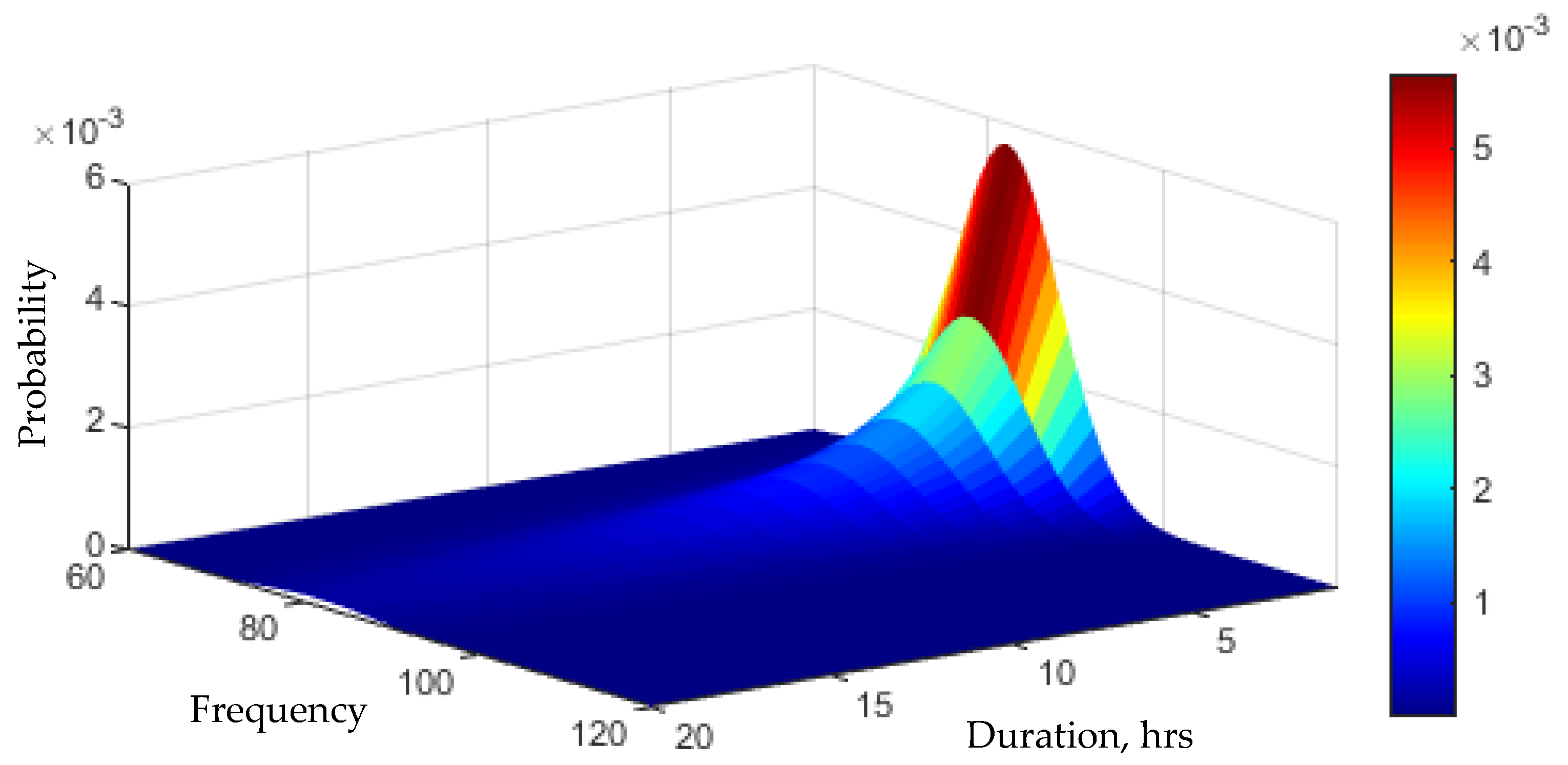

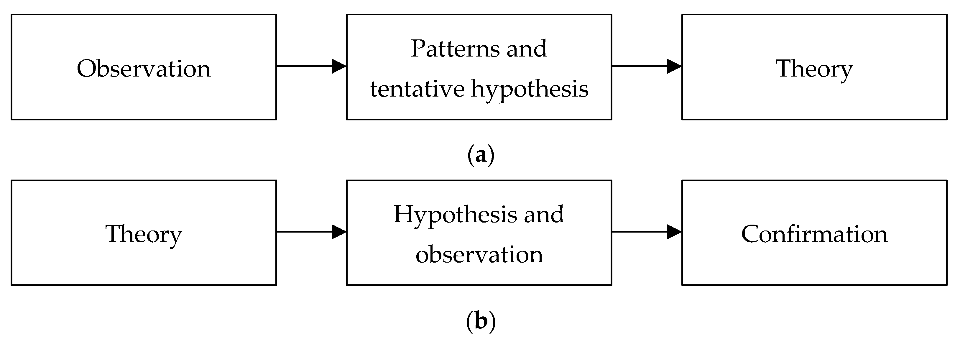
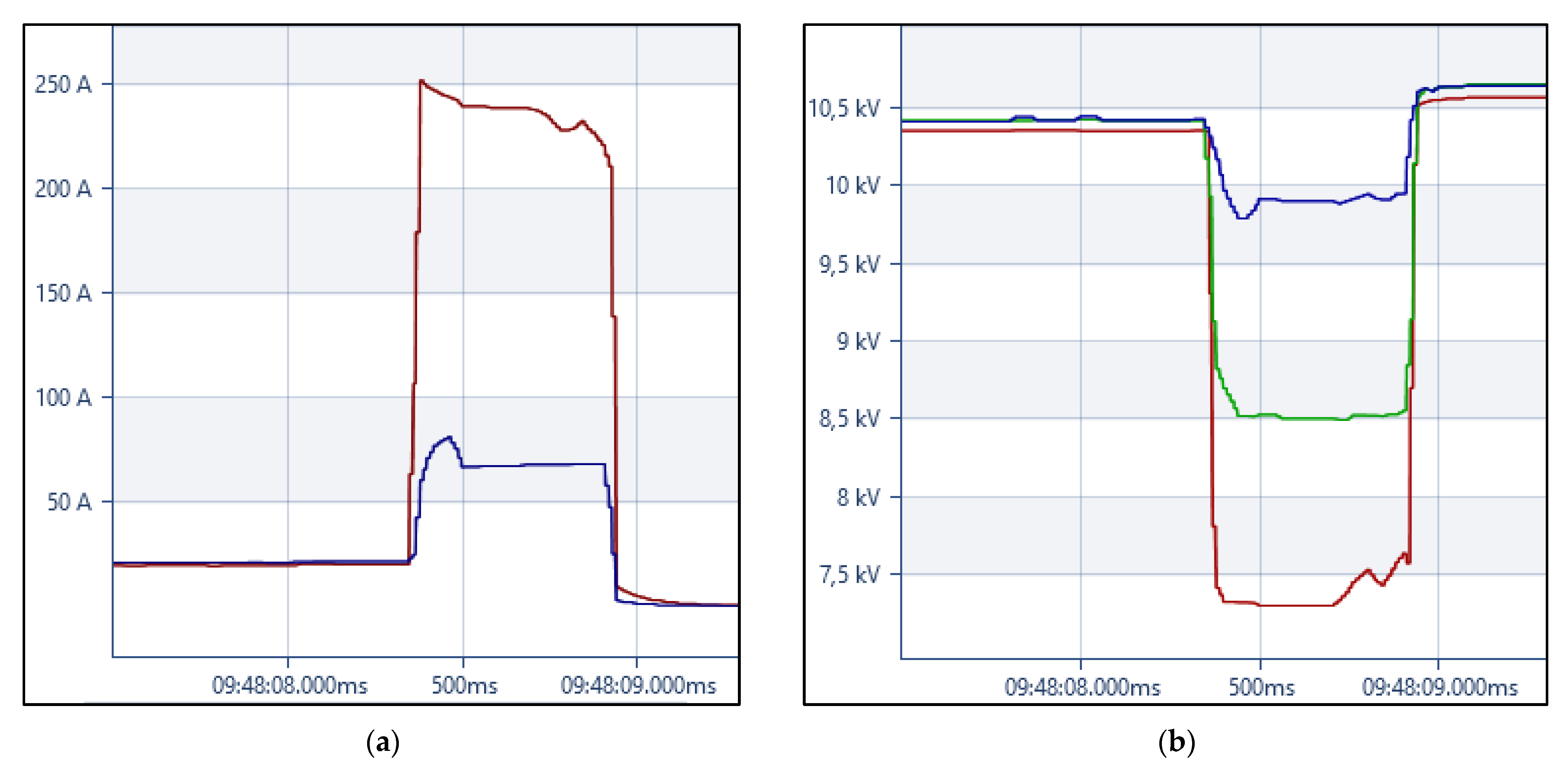

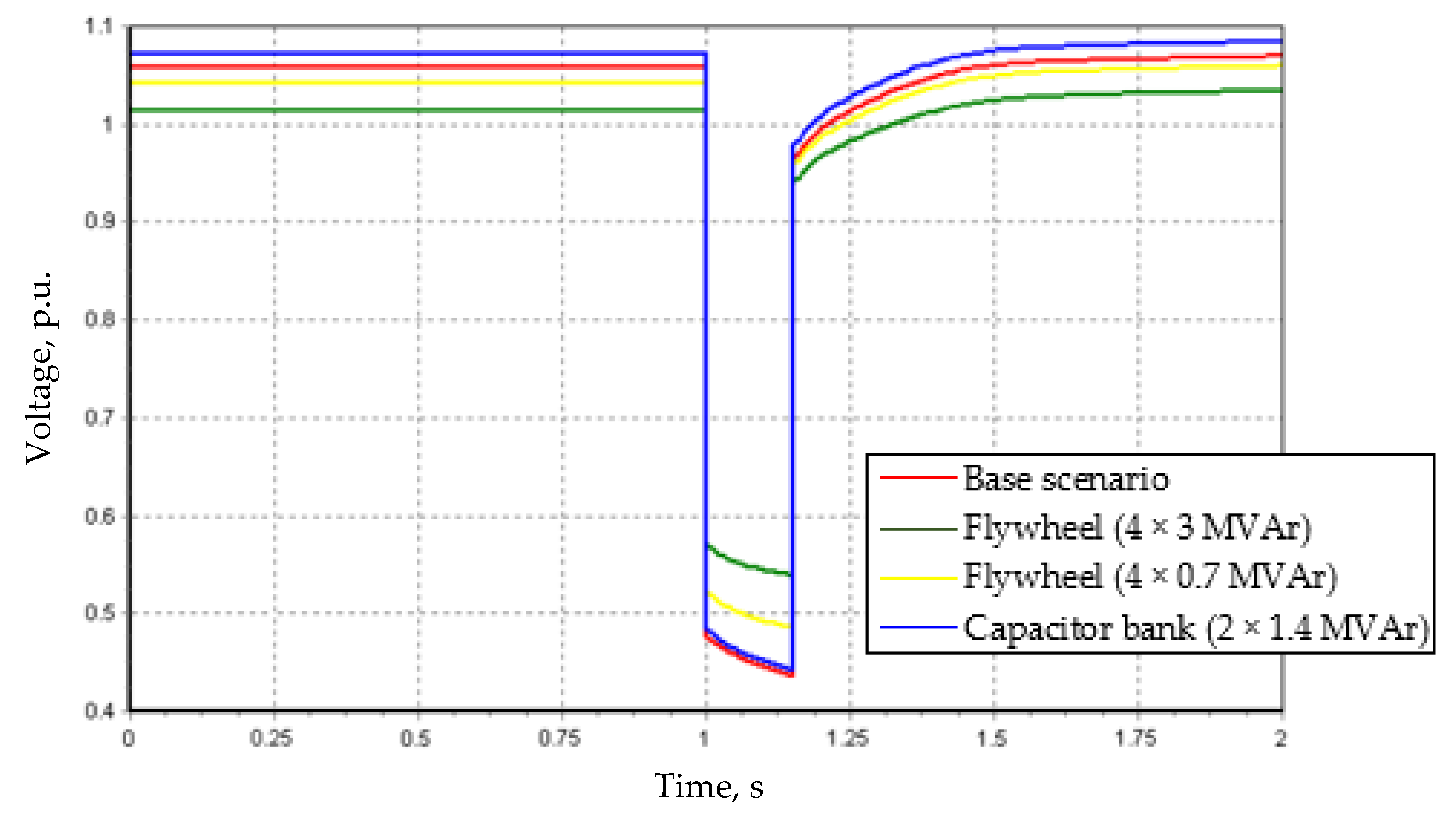

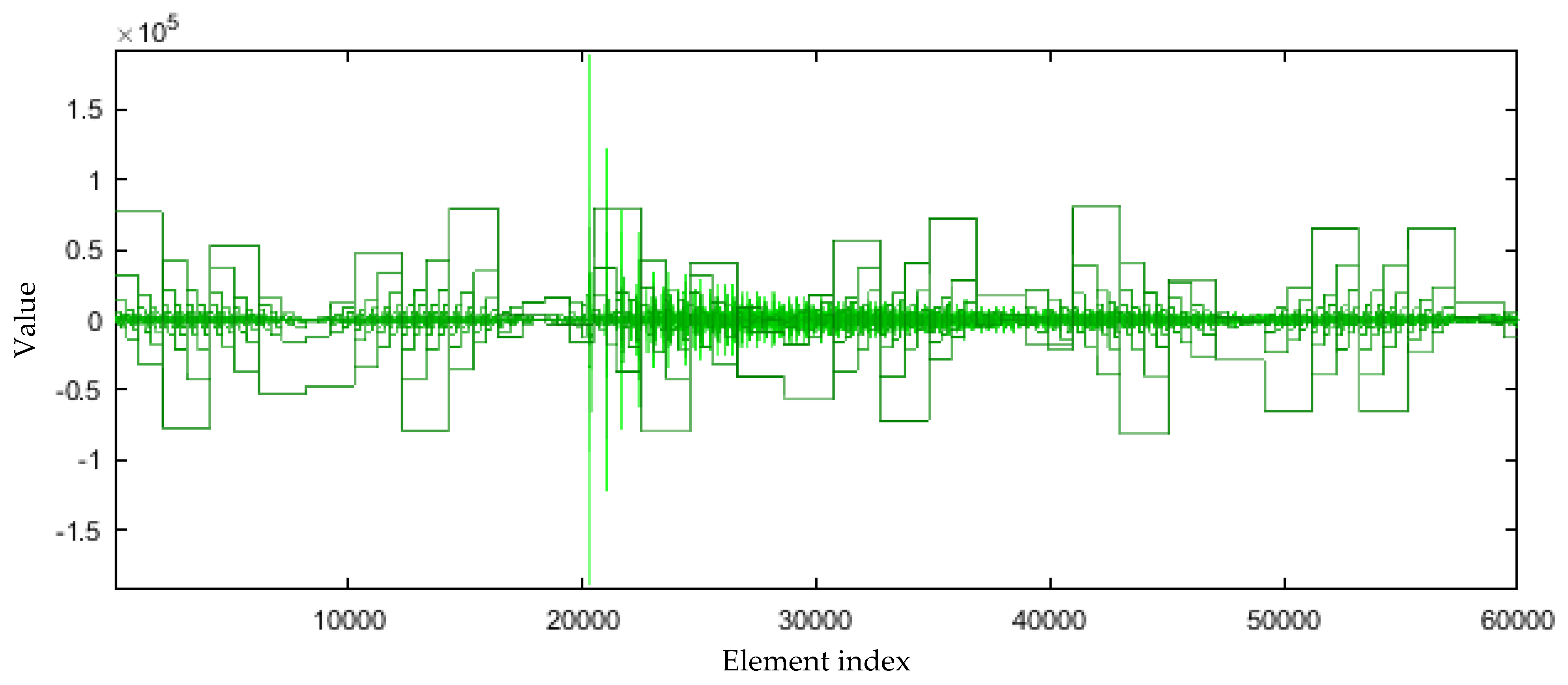
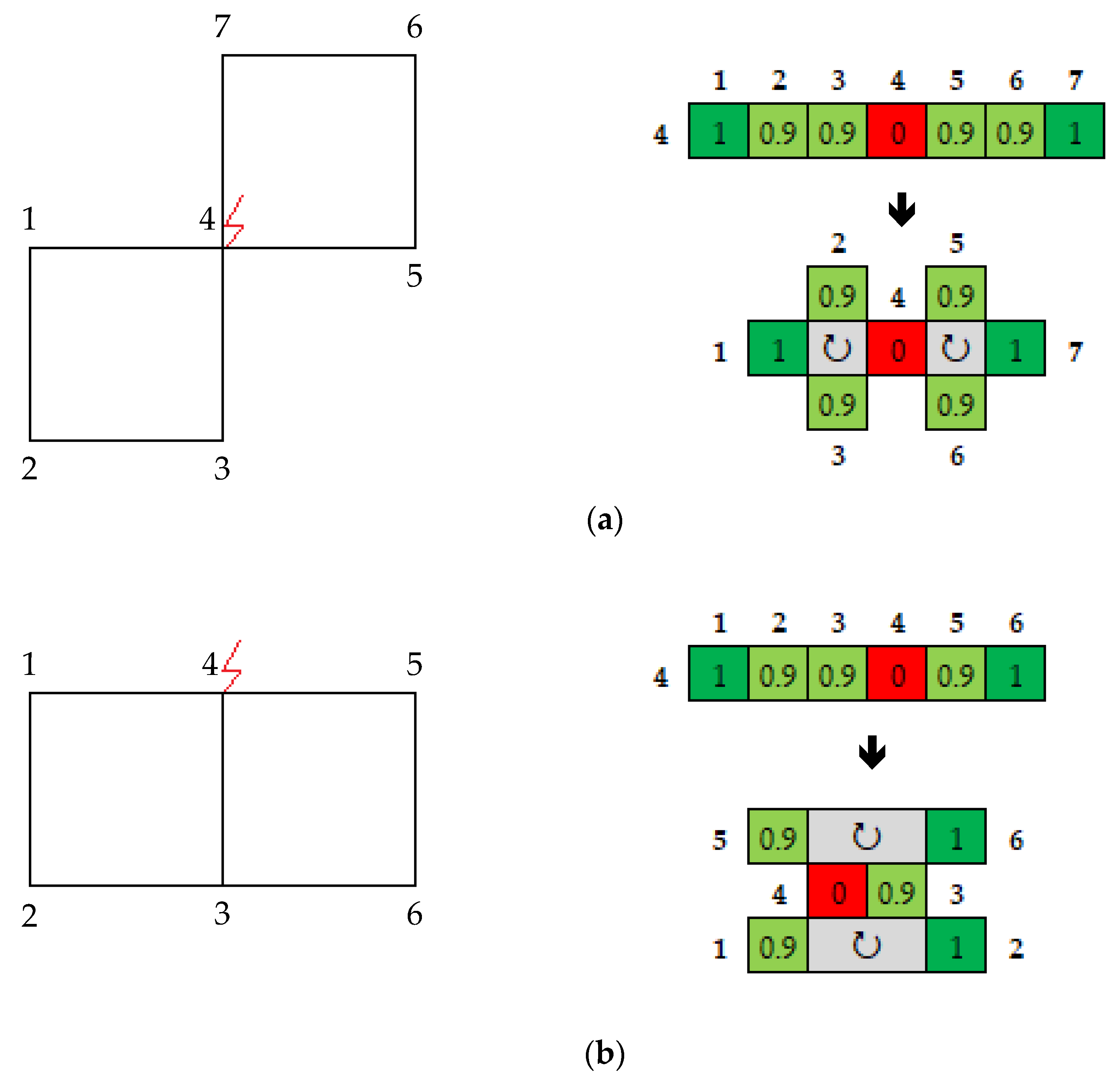
Disclaimer/Publisher’s Note: The statements, opinions and data contained in all publications are solely those of the individual author(s) and contributor(s) and not of MDPI and/or the editor(s). MDPI and/or the editor(s) disclaim responsibility for any injury to people or property resulting from any ideas, methods, instructions or products referred to in the content. |
© 2023 by the authors. Licensee MDPI, Basel, Switzerland. This article is an open access article distributed under the terms and conditions of the Creative Commons Attribution (CC BY) license (https://creativecommons.org/licenses/by/4.0/).