Research on Detection and Restoration Methods of Basic Operation Data for Inter-Basin Water Diversion Projects

Abstract

Inter-basin water diversion is an essential means to alleviate the contradiction between the supply and demand of water resources, and accurate hydraulic modelling guarantees smooth operation. However, due to the increasing complexity of water diversion methods, structures, water conservancy facilities and equipment, it is difficult to obtain accurate and effective measured data to establish a model. Therefore, based on a data-driven method, this paper diagnoses and restores the important parameters of the water diversion projects, including the elevation of pipeline and water level data, which can be used to establish the adaptive hydraulic transition model of the water diversion projects. Firstly, the abnormal data of the elevation of pipeline were identified using expert data annotation and support vector classification (SVC), with the identification accuracy of abnormal data being as high as 91%. Then, the single and continuous abnormal data were restored using an interpolation method and multiple linear regression algorithm (MLR), and the restored data were found to be consistent with the judgment of expert knowledge. Secondly, K-medoids was used to classify the complex multi-dimensional water level data, combined with the 3-sigma method to identify the outliers in each class. The gradient boosting decision tree algorithm (GBDT) trained on normal data restored outliers in a predictive manner, and the mean absolute percentage error (MAPE) was 0.003%, 0.025% and 0.091% in each class, respectively, showing the best accuracy compared with other models.

1. Introduction

In recent years, global climate change and human activities have intensified the pressure on water resources and terrestrial aquatic systems, and the spatiotemporal distribution of global freshwater resources is continuously expanding [1,2]. Thus, to solve the conflict between the supply and demand of water in water-scarce areas, the construction of inter-basin water diversion projects is considered a common and direct engineering means to alleviate the scarcity of water in parched regions [3,4]. However, it is an increasing concern that inter-basin water diversion projects may cause some negative environmental and societal impacts [5,6,7,8]. Despite some controversy, many countries are still committed to providing sufficient water supply for their economies through the construction of cross-basin water transfer projects [9,10,11]. For instance, more than 40 countries and regions around the world have completed over 350 water diversion projects [12], with an annual water diversion scale exceeding 540 billion cubic meters at the end of 2021 [1]. However, in the past few decades, due to factors such as the terrain, geology, and water diversion scale along the route as well as the increasingly complicated water diversion methods, structures, and water conservancy facilities and equipment involved, the operational safety of inter-basin water diversion projects has been greatly challenged.

Water hammer usually occurs during hydraulic transients in pipeline systems and leads to severe damage and vibration [13,14], such as erosion, cavitation, pipeline rupture and even collapse [15,16]. Since the undesirable phenomenon of water hammer poses a threat to daily routine safety in inter-basin water diversion projects, two methods are usually adopted to predict and prevent water hammer issues, including physical simulation and numerical simulation [17,18]. The rapid development of information technologies has accelerated the promotion of numerical simulation in the scope of water hammer prevention. Over the past few decades, to study transient flow issues in inter-basin water diversion projects, a variety of numerical simulation methods have been continuously developed, such as MOC (the method of characteristics) [13], WCM (wave characteristic method) [16], FVM (finite volume method) [19,20], FEM (finite element method) [21] and FDM (finite difference method) [22]. The explicit method of characteristics is usually adopted in the simulation of complex pipeline systems [23]. In addition, MOC is typically used to simulate transient flow processes of complicated pipe systems with air chambers, valves, and pumps [24,25,26,27].

Recently, research on the application of hydrological information monitoring data has been constantly emerging. Traditionally, actual measured data on the discharge and water level can be utilized for real-time constraints, calibration, and validation of hydraulic models [28]. For instance, the hydrological monitoring data of the water level and flow are the basis for decision-making in the field of flood forecasting [29]. Kim et al. pointed out that the real-time collection of water level and rainfall data is beneficial for the application of machine learning algorithms and ensures continuous learning [30].

In addition, in the process of water regime data monitoring of water diversion projects, a variety of factors, such as transmission and manual recording errors of data, monitoring facility failures and network equipment faults, may induce the frequent occurrence of abnormal data [31,32], which was found to have an influence on the determination and optimization for daily operation schemes and even trigger higher water supply costs [33]. In order to conduct quantitative research on the uncertainty of drainage systems, Chen et al. proposed an evaluation method for the degree of rainwater inlet blockage based on multi-hydrological monitoring data [34]. Over the past few decades, the extension of artificial intelligence technology to various fields inaugurated a new era in artificial intelligence development. For instance, in order to improve the accuracy of hydrological monitoring, Fu et al. proposed an anomaly identification method for hydrological monitoring data based on an improved random forest algorithm [35]. Tabari and Talaee [36] examined the efficiency of the multilayer perceptron (MLP) and radial basis function (RBF) networks for recovering the missing values of 13 water quality parameters based on data from five stations located along the Maroon River, Iran. Ratolojanahary et al. [37] combined MICE (multivariate imputations by chained equations) with random forest (RF), boosted regression trees (BRT), K-nearest neighbors (KNN) and support vector regression (SVR) to address the issue of data imputation in the context of water quality assessment.

Previous studies have shown that machine learning technology has been applied to data mining in water diversion projects and has achieved good results. However, existing research is insufficient. For instance, the lack of integration between professional knowledge and data-driven methods may lead to issues such as low accuracy and poor interpretability of diagnostic results. It is also the main reason that basic data processing before modeling still heavily relies on manual methods to eliminate or recover abnormal data in current engineering practice. Therefore, this paper innovatively integrates professional knowledge with data analysis methods and proposes a method for detecting and restoring the basic data before establishing adaptive hydraulic transient models of water diversion projects. In addition, to provide prepared data support for the establishment of hydraulic transient models for water diversion projects, the practicality of five machine learning prediction models has been compared and analyzed in this paper, namely the support vector machine algorithm (SVM), artificial neural network algorithm (ANN), random forest algorithm (RF), gradient boosting decision tree algorithm (GBDT) and multiple linear regression algorithm (MLR).

2. Methods

2.1. Study Area

As a crucial component of the “T”-shaped water diversion artery in the East Route, the Jiaodong Water Diversion Project is committed to achieving optimal allocation of water throughout Shandong province, solving the supply–demand contradiction of fresh water in the Shandong region and improving the local ecological environment. The total length of the water conveyance line of this project is 469.2 km, with 9 levels of water pumping stations, 5 water conveyance tunnels, 6 large aqueducts, and 461 hydraulic facilities, including water gates, inverted siphons, and bridges. Among them, the total length of the section from Gaotuan Pump Station to Mishan Reservoir is 95.16 km, including 2 pump stations, 5 sections of pressure conduit with an elevated tank and a regulating tank, 2 non-pressure tunnel sections and 1 pressurized tunnel section. The cross-sectional configuration of this project is shown in Figure 1. In addition, to ensure the safe operation and reasonable regulation of inter-basin water diversion projects, a comprehensive data network of monitoring stations is indispensable for collecting real-time data, including discharge, water level and other necessary data of important hydraulic facilities at various points along the route.

2.2. Methodology

2.2.1. Identification Method

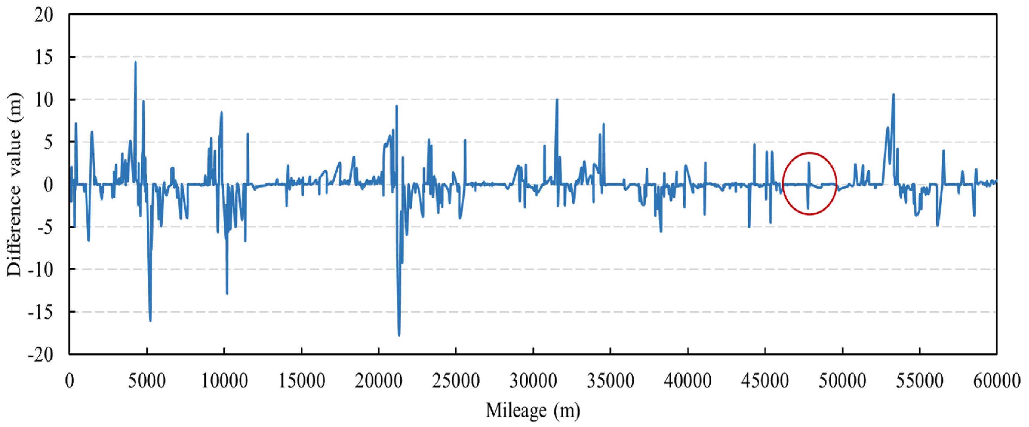
Data-driven methods are used to identify abnormal data and restore them. For the collected data on the elevation of pipeline, some of the data are judged and identified via expert knowledge, and the labels 0 and 1 are assigned to abnormal data and normal data. The classification model is then trained based on the labeled data, which are used to identify other data for the elevation of pipeline. Before model training, additional input features are constructed to assist the training of the classification model. The difference method is used to construct the new feature, i.e., the difference between the data and the last data. The nearby data of the data point are used as input features at the same time to give the model a better understanding of the sequential data. The support vector machine classifier is used in this model.

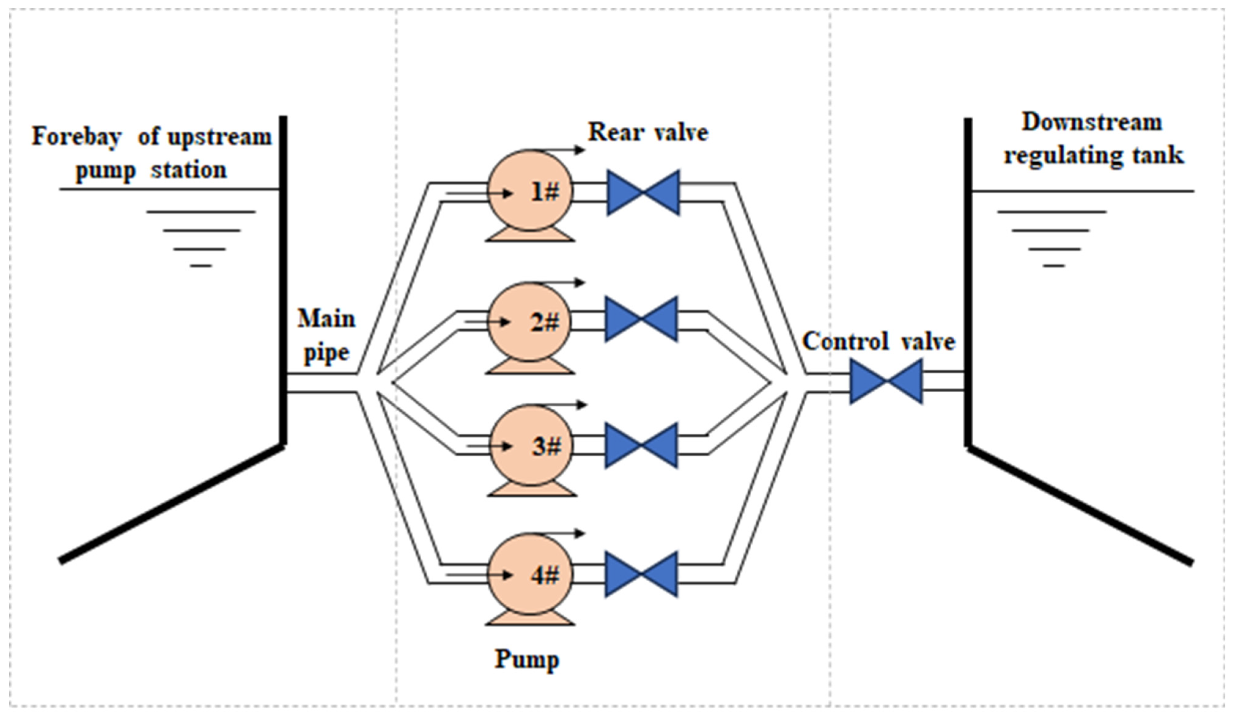
For water level data, there are many influence factors (e.g., water flow, water level, pump frequency and valve opening at nearby nodes) and various operation patterns, so it is difficult to directly identify abnormal data. Therefore, in the judgment of abnormal water level data, the clustering algorithm is used to cluster the data first, and then the abnormal data are identified by the 3-sigma method according to different operation patterns.

The clustering algorithm uses the K-medoids algorithm, which is an improvement on K-means clustering. Instead of using the mean, K-medoids clustering uses the most central object in the cluster, that is, the medoid, as the reference point, and that of each selection must be a sample point.

When there are noise and isolated points, K-medoids is more robust than K-means, but the time complexity of calculating the centroid step is O(n2), and the running speed is relatively slow. The basic idea of the algorithm is to divide the observed objects into several subsets, and each subset is regarded as a class, so the objects within the class are similar and the objects between the classes are not similar. The steps are as follows:

• Input the data to be clustered and randomly select K points in the data as the centroids.
• Aggregate all data points in the dataset into the closest cluster based on the distance to the centroid.
• Compute the distance between each cluster point as a centroid, and then choose the point with the smallest distance as the new centroid. Repeat steps 2 and 3 until the centroids of every cluster no longer change or the sum of squared errors (convergence function) is minimized. The sum of squared errors (SSE) is calculated as follows:

$$\mathrm{SSE}={{\displaystyle \sum }}_{\mathrm{i}=1}^{\mathrm{k}}{{\displaystyle \sum }}_{\mathrm{p}\in {\mathrm{C}}_{\mathrm{i}}}{\left|{\mathrm{p}-\mathrm{m}}_{\mathrm{i}}\right|}^2$$

(1)

where ${\mathrm{C}}_{\mathrm{i}}$ is the ith cluster, p is sample data points in ${\mathrm{C}}_{\mathrm{i}}$, and ${\mathrm{m}}_{\mathrm{i}}$ is the centroid of ${\mathrm{C}}_{\mathrm{i}}$. The smaller the SSE of each cluster, the higher the overall compactness of the data around the centroid in each cluster under this clustering condition, and the better the clustering effect.

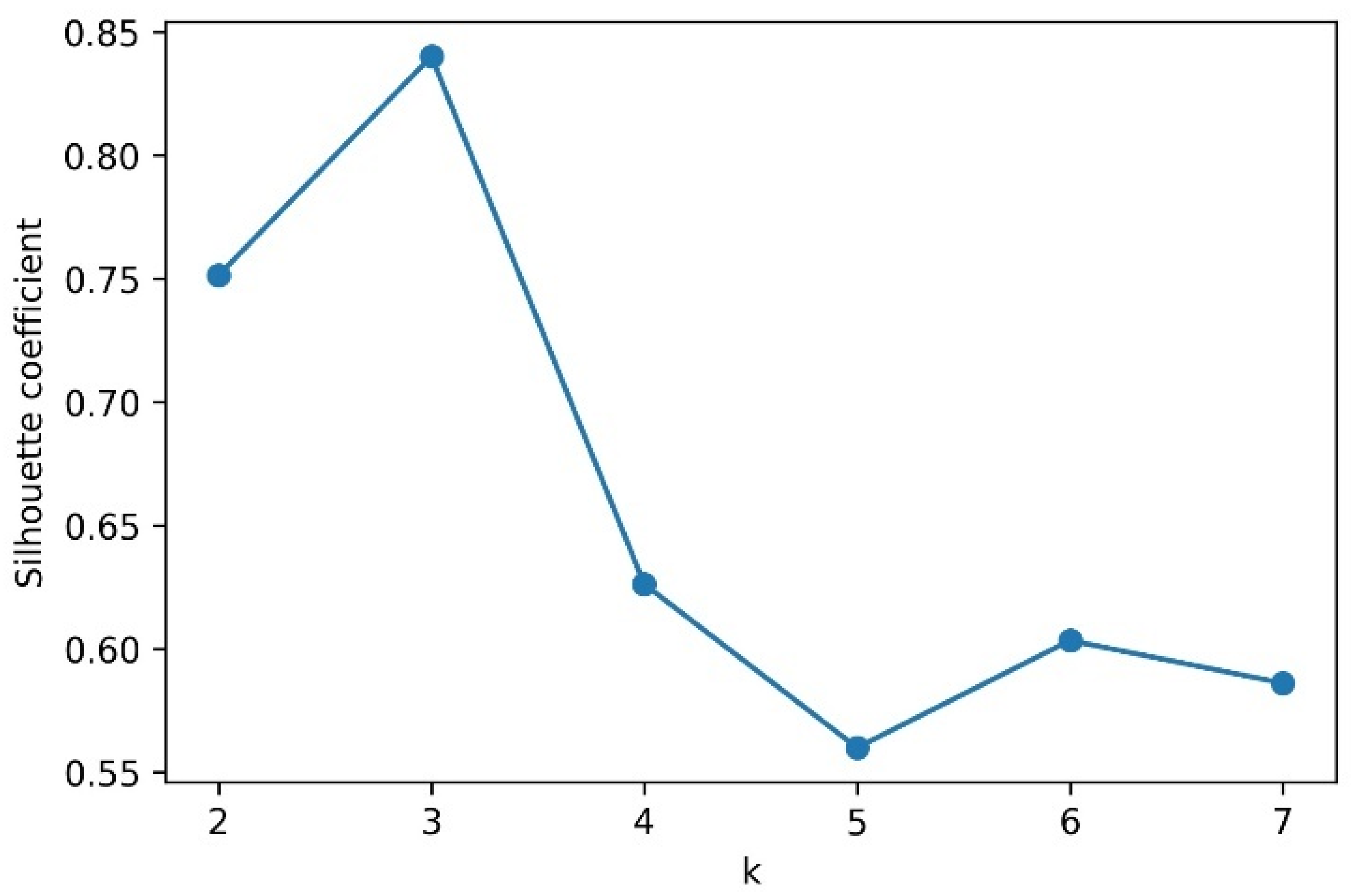
It is very important to find the optimal value of K for the k-medoids algorithm. The silhouette coefficient is adopted in this paper, and its basic principle is as follows: first, the intra-cluster similarity $\mathrm{a}\left(\mathrm{i}\right)$ of the sample is calculated, which represents the average distance between the sample and other sample points in the same cluster. The smaller the value, the more correct the classification. Then, the dissimilarity measure $\mathrm{b}\left(\mathrm{i}\right)$ is computed, which is the average distance between the sample and the other clusters. Higher values indicate better classification. Therefore, the calculation method of $\mathrm{Silhouette}\left(\mathrm{i}\right)$ is as follows:

$$\mathrm{Silhouette}(\mathrm{i})=\left\{\begin{array}{cc}\hfill 1-\frac{\mathrm{a}\left(\mathrm{i}\right)}{\mathrm{b}\left(\mathrm{i}\right)}& \hfill \mathrm{a}(\mathrm{i}) < \mathrm{b}(\mathrm{i})\\ \hfill 0& \hfill \mathrm{a}\left(\mathrm{i}\right)=\mathrm{b}\left(\mathrm{i}\right)\\ \hfill \frac{\mathrm{b}(\mathrm{i})}{\mathrm{a}(\mathrm{i})}-1& \hfill \mathrm{a}(\mathrm{i})>\mathrm{b}(\mathrm{i})\end{array}\right.$$

(2)

where $\mathrm{Silhouette}(\mathrm{i})$ and $\mathrm{a}(\mathrm{i})$ represent the coefficient of silhouette and the intra cluster similarity, respectively, and $\mathrm{b}(\mathrm{i})$ is the dissimilarity between the sample and other clusters. $\mathrm{Silhouette}(\mathrm{i})$ is a number in the range [−1, 1], and the closer $\mathrm{Silhouette}(\mathrm{i})$ is to 1, the more reasonable the cluster is. In general, when the silhouette coefficient > 0.5, the clustering can achieve a relatively ideal effect. When the silhouette coefficient < 0.2, the clustering effect is poor.

2.2.2. Restoration Method

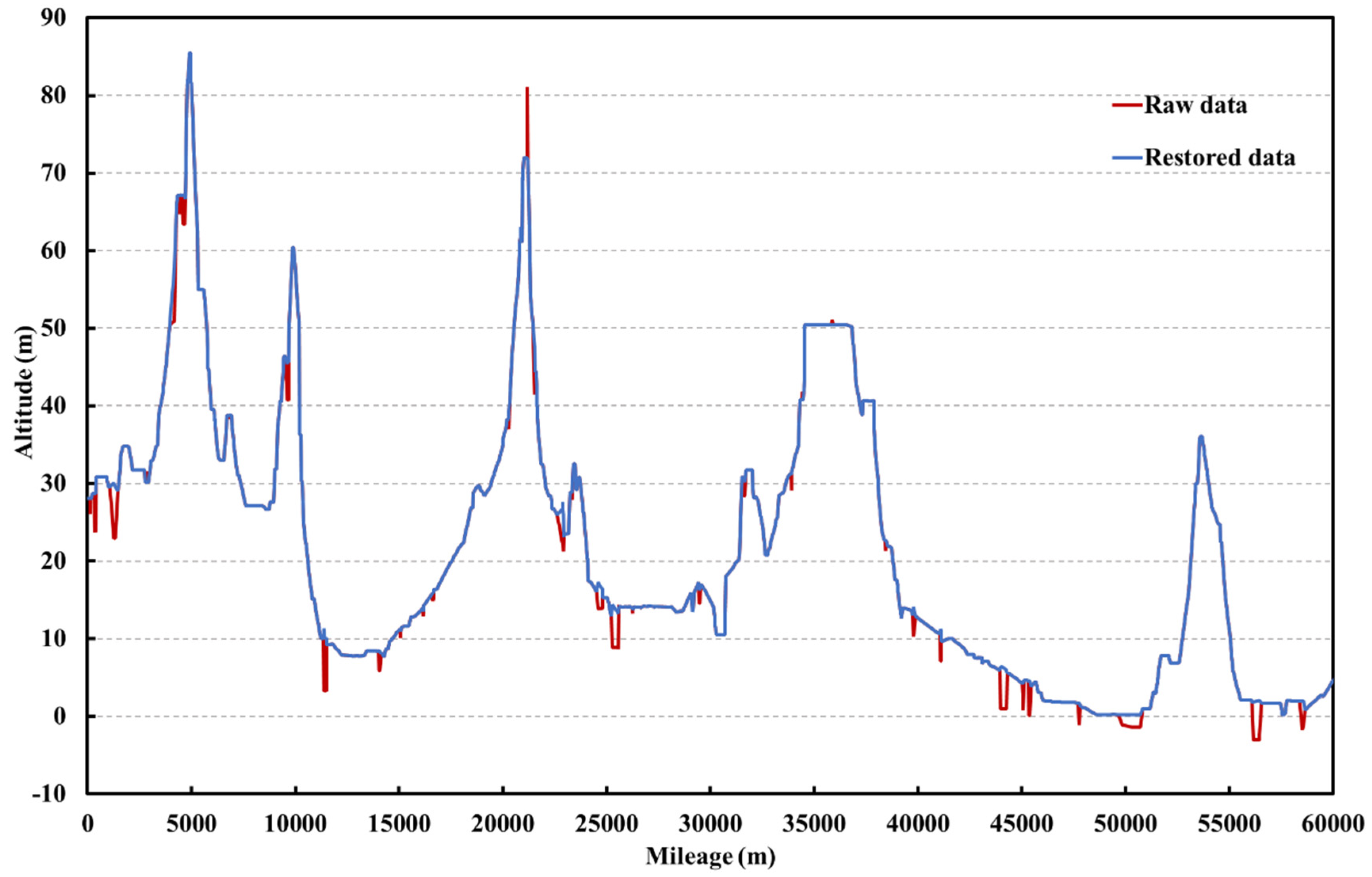
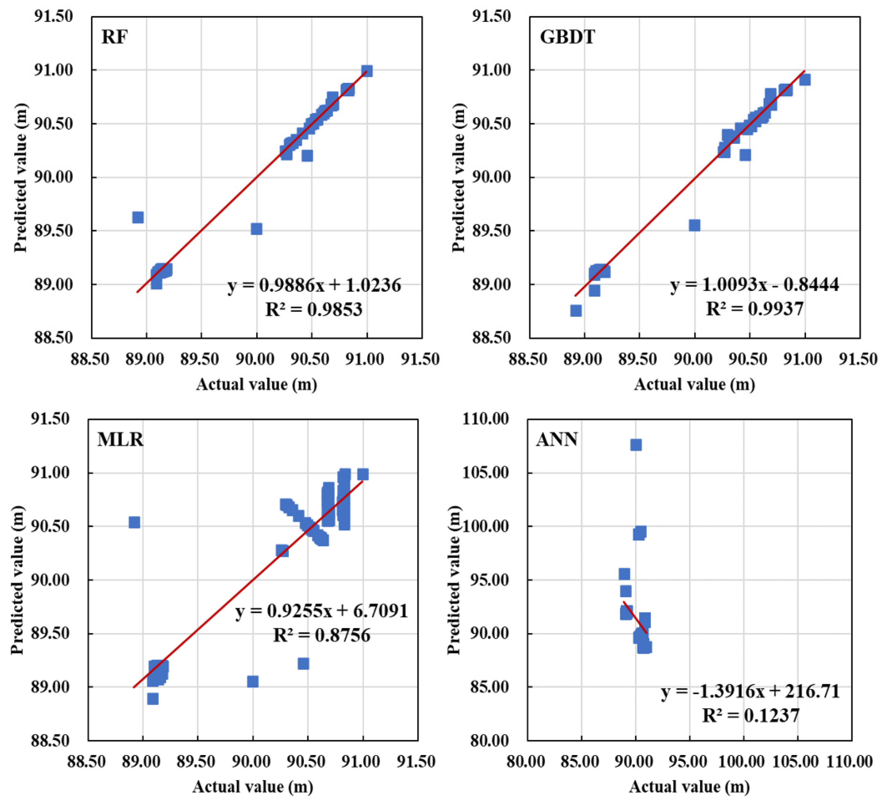
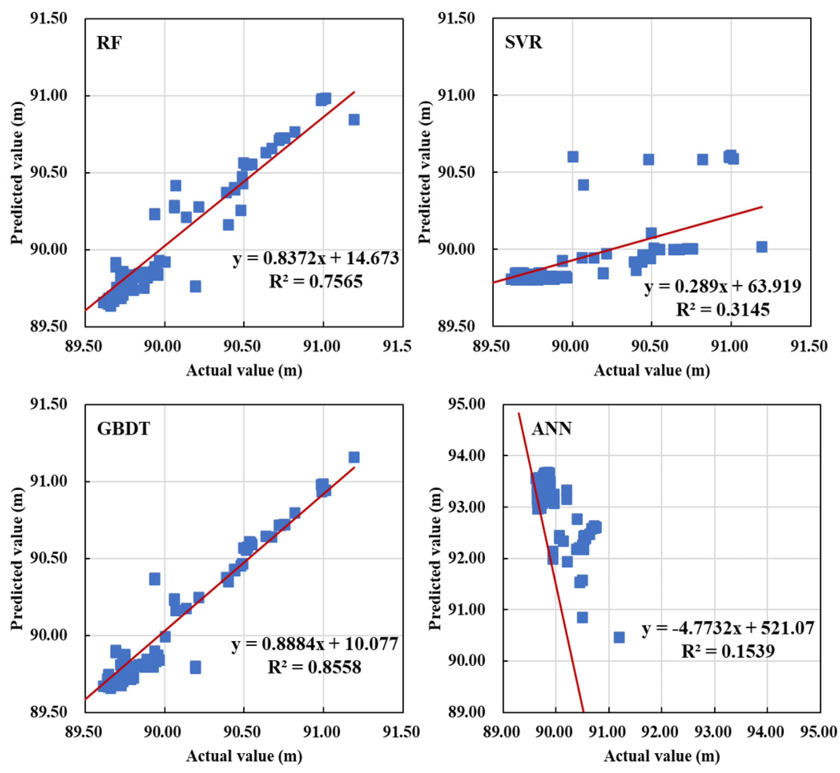
For the single outlier data in the data for the elevation of pipeline (i.e., one-dimensional data), the mean method is used to restore it, and for the continuous outliers, the machine learning prediction model is used to restore it. For the water level data, the prediction model of each cluster is established to restore water level data.

MLR, RF, ANN, GBDT and SVM are used as prediction models. The algorithm works as follows:

SVM is a supervised machine learning algorithm that can be used for the classification of discrete dependent variables and the prediction of continuous dependent variables. In general, this algorithm will have better prediction accuracy than other single classification algorithms, mainly because it can convert a low-dimensional linearly indivisible space to a high-dimensional linearly separable space by the kernel function. For the nonlinear SVM model, it is necessary to go through two steps; one is to map the sample points in the original space to the new space of high latitude, and the other is to find a linear “hyperplane” in the new space for identifying various sample points.

Common Liner kernel functions:

$$\mathrm{K}\left({\mathrm{x}}_{\mathrm{i}}{, \mathrm{x}}_{\mathrm{j}}\right){=\mathrm{x}}_{\mathrm{i}}·{\mathrm{x}}_{\mathrm{j}}$$

(3)

Polynomial kernel functions:

$$\mathrm{K}\left({\mathrm{x}}_{\mathrm{i}}{, \mathrm{x}}_{\mathrm{j}}\right)={\left(\mathsf{\gamma }\left({\mathrm{x}}_{\mathrm{i}}·{\mathrm{x}}_{\mathrm{j}}\right)+\mathrm{r}\right)}^{\mathrm{p}}$$

(4)

RBF kernel functions:

$$\mathrm{K}\left({\mathrm{x}}_{\mathrm{i}}{, \mathrm{x}}_{\mathrm{j}}\right){=\mathrm{e}}^{\left(-\mathsf{\gamma }\Vert {\mathrm{x}}_{\mathrm{i}}-{\mathrm{x}}_{\mathrm{j}}\Vert {}^2\right)}$$

(5)

Sigmoid kernel functions:

$$\mathrm{K}\left({\mathrm{x}}_{\mathrm{i}}{, \mathrm{x}}_{\mathrm{j}}\right)=\tan \mathrm{h}\left(\mathsf{\gamma }\left({\mathrm{x}}_{\mathrm{i}}·{ \mathrm{x}}_{\mathrm{j}}\right)+\mathrm{r}\right)$$

(6)

In practical applications, the selection of kernel functions is the key to the calculation of support vector machine models. Thus, it is important to combine prior domain knowledge with a cross-validation method to elect a reasonable kernel function. The SVM method has been applied in many fields due to its strong applicability and simple process.

RF is a tree-based algorithm, which builds multiple classification trees and fuses their results to obtain better performance. The results of all decision trees are averaged as the final prediction result of the model for regression problems. Random forest adopts the idea of Bootstrap aggregating (Bagging) in ensemble learning. It randomly extracts samples and features from the sample set and trains a tree based on them, making each tree in the forest unique and different. Random forests are efficient because the trees can be run in parallel, and they overcome the instability problem of a single decision tree. In addition, random forests can handle high-dimensional datasets with high accuracy. The specific calculation steps of RF are as follows:

• Construct N decision trees from original samples by Bootstrap method;
• Select M features in the m dimension and select the best features as split nodes to establish different decision trees, where m < M;
• Do not prune the decision tree, so as to ensure that the decision tree grows as much as possible;
• Calculate the average value from the results of each decision tree as the final output result of the random forest, as shown in Equation (7).

  $${\mathrm{F}}_{\mathrm{RF}}\left(\mathrm{X}\right)=\frac{1}{\mathrm{N}}{{\displaystyle \sum }}_1^{\mathrm{N}}{\mathrm{T}}_{\mathrm{k}}\left(\mathrm{x}\right)$$

  (7)

GBDT is an iterative decision tree algorithm, which is composed of multiple decision trees, and the final result is made by summing up the results of all trees. The tree in GBDT is a regression tree, not a classification tree, and GBDT is mainly used for regression prediction.

In the training process, it uses the non-positive gradient of loss function as the approximation of the foundation model loss in the mth round of the foundation model, and then uses this approximation value to build the next round of the foundation model. The calculation of the approximate residual of the negative gradient value of the loss function is an expansion of the gradient lifting algorithm on the lifting algorithm, which makes the objective function more convenient to solve.

The steps are as follows:

1. Find a constant that minimizes the loss function and initialize a tree with only the root node.

2. Calculate the negative gradient of the loss function and use it as an estimate of the residual

$${\mathrm{r}}_{\mathrm{mi}}=-{\left[\frac{\partial \left({\mathrm{y}}_{\mathrm{i}}, \mathrm{f}\left({\mathrm{x}}_{\mathrm{i}}\right)\right)}{\partial \mathrm{f}\left({\mathrm{x}}_{\mathrm{i}}\right)}\right]}_{\mathrm{f}\left(\mathrm{x}\right){=\mathrm{f}}_{\mathrm{m}-1}\left(\mathrm{x}\right)}$$

(8)

3. Using the data set $\left({\mathrm{x}}_{\mathrm{i}}{, \mathrm{r}}_{\mathrm{mi}}\right)$-based model fitting the next round, have corresponding J a leaf node ${\mathrm{R}}_{\mathrm{mj}}$, J = 1, 2, 3, …, J − 1, J. The residual value ${\mathrm{r}}_{\mathrm{mi}}$ can be estimated using ${\mathrm{R}}_{\mathrm{mj}}$, namely the optimal fitting value of every single leaf node. The mth base model $f_m\left(x\right)$ predicts the following value at leaf node j.

$${\mathrm{c}}_{\mathrm{mj}}{=\mathrm{argmin}}_{\mathrm{c}}{{\displaystyle \sum }}_{{\mathrm{x}}_{\mathrm{i}}\in {\mathrm{R}}_{\mathrm{mj}}}\mathrm{L}\left({\mathrm{y}}_{\mathrm{i}}{, \mathrm{f}}_{\mathrm{m}-1}\left({\mathrm{x}}_{\mathrm{i}}\right)+\mathrm{c}\right)$$

(9)

4. The base model ${\mathrm{f}}_{\mathrm{m}}\left(\mathrm{x}\right)$ of the mth round is obtained, and the gradient boosting model is obtained by integrating the base model of the previous m − 1 rounds.

$${\mathrm{F}}_{\mathrm{M}}\left(\mathrm{x}\right){=\mathrm{F}}_{\mathrm{M}-1}\left(\mathrm{x}\right){+\mathrm{f}}_{\mathrm{m}}\left(\mathrm{x}\right)={{\displaystyle \sum }}_{\mathrm{m}=1}^{\mathrm{M}}{{\displaystyle \sum }}_{\mathrm{j}=1}^{\mathrm{J}}{\mathrm{c}}_{\mathrm{mj}}\mathrm{I} \left({\mathrm{x}}_{\mathrm{i}}\in {\mathrm{R}}_{\mathrm{mj}}\right)$$

(10)

ANN is a network model abstracted from the perspective of information processing by imitating the structure of the human or animal nervous system. The basic structure of a simple neuron consists of a weight vector W, an input vector x and an activation function. The calculation is expressed as follows:

$$\mathrm{a}=\mathrm{f}\left({\mathrm{W}}^{\mathrm{T}}\mathrm{x}+\mathrm{b}\right)$$

(11)

A simple ANN usually contains an input layer, hidden layer, and output layer. In order to obtain high-level abstract features, complex neural networks usually use multiple hidden layers. Neurons in the same layer are not connected to each other, while neurons in adjacent layers are pairwise connected through a weight matrix that reflects the degree of influence of the output of the upper-layer neurons on the input of the lower-layer neurons. This connection method also abstracts the relationship between adjacent layers into the product form of the weight matrix and the input neuron vector. The relationship between the neuron output of layer l − 1 and the neuron output of layer l is expressed as Equations (12) and (13).

$${\mathrm{z}}^{\left(\mathrm{l}\right)}={\mathrm{W}}^{\left(\mathrm{l}\right)}{\mathrm{a}}^{\left(\mathrm{l}-1\right)}+{\mathrm{b}}^{\left(\mathrm{l}\right)}$$

(12)

$${\mathrm{a}}^{\left(\mathrm{l}\right)}={\mathrm{f}}^{\left(\mathrm{l}\right)}\left({\mathrm{z}}^{\left(\mathrm{l}\right)}\right)$$

(13)

where $n_l$ is the number of neurons in layer l and $a^{\left(l-1\right)}$ is the output vector of neurons in layer L − 1, which is also used as the input vector of layer l. $W^{\left(l\right)}\in {ℝ}^{n_l\times n_{l-1}}$ is the connection weight matrix from layer L − 1 to layer l. $b^{\left(l\right)}\in {ℝ}^{n_l}$ is the bias vector of the $l\mathrm{th}$ layer, $z^{\left(l\right)}$ is the output of the $l\mathrm{th}$ layer before activation, $f^{\left(l\right)}$ is the nonlinear activation function, and $a^{\left(l\right)}$ is the activated neuron vector used as the output of layer l, and the input of layer l + 1.

Equations (12) and (13) constitute the feedforward calculation part of the model, that is, the iterative calculation process of the input passing from the input to the output layer in turn. On the basis of feedforward calculation, the model compares the predicted value obtained by feedforward calculation with the actual value through the error backpropagation algorithm to calculate the error gradient, and then backpropagates these errors layer by layer by changing the weight and bias of each neuron to finally produce the output of the network model.

Multiple linear regression (MLR) is a statistical method that describes the linear relationship between variables. Due to the ability to predict the dependent variable by introducing the optimal combination of multiple independent variables, MLR is more effective than univariate linear regression models that only use one independent variable. The prediction model is expressed as follows:

$${\mathrm{y}}_{\mathrm{a}}={\mathsf{\beta }}_0+{\mathsf{\beta }}_1{\mathrm{x}}_1+{\mathsf{\beta }}_2{\mathrm{x}}_2+\dots +{\mathsf{\beta }}_{\mathrm{k}}{\mathrm{x}}_{\mathrm{k}}+ϵ$$

(14)

Since the observations of multiple linear regression are a vector instead of a scalar, a matrix is introduced to represent these observations, as shown in Equation (15). The matrix form of multiple linear regression is shown in Equation (16).

$$\mathrm{X}=\left[\begin{array}{cc}\begin{array}{cc}1& {\mathrm{x}}_{11}\\ 1& {\mathrm{x}}_{21}\end{array}& \begin{array}{cc}\cdots & {\mathrm{x}}_{1\mathrm{k}}\\ \cdots & {\mathrm{x}}_{2\mathrm{k}}\end{array}\\ \begin{array}{cc}⋮& ⋮\\ 1& {\mathrm{x}}_{\mathrm{n}1}\end{array}& \begin{array}{cc}\ddots & ⋮\\ \cdots & {\mathrm{x}}_{\mathrm{nk}}\end{array}\end{array}\right],\mathrm{Y}=\left[\begin{array}{c}\begin{array}{c}{\mathrm{y}}_1\\ {\mathrm{y}}_2\end{array}\\ \begin{array}{c}⋮\\ {\mathrm{y}}_{\mathrm{n}}\end{array}\end{array}\right],\mathsf{\beta }=\left[\begin{array}{c}\begin{array}{c}{\mathsf{\beta }}_1\\ {\mathsf{\beta }}_2\end{array}\\ \begin{array}{c}⋮\\ {\mathsf{\beta }}_{\mathrm{n}}\end{array}\end{array}\right],ϵ=\left[\begin{array}{c}\begin{array}{c}{ϵ}_1\\ {ϵ}_2\end{array}\\ \begin{array}{c}⋮\\ {ϵ}_{\mathrm{n}}\end{array}\end{array}\right]$$

(15)

$$\mathrm{Y}=\mathrm{X}\mathsf{\beta }+ϵ$$

(16)

2.3. Evaluation Criteria

In this paper, precision and accuracy are utilized to evaluate the performance of classification models. Precision is a measure of how many of the samples predicted to be positive are genuinely positive. The accuracy is the fraction of samples that are correctly predicted.

$$\mathrm{Accuracy}=\frac{\mathrm{TP}+\mathrm{TN}}{\mathrm{TP}+\mathrm{FN}+\mathrm{TN}+\mathrm{FP}}$$

(17)

$$\mathrm{Precision}=\frac{\mathrm{TP}}{\mathrm{TP}+\mathrm{FP}}$$

(18)

The root mean square error (RMSE), mean absolute error (MAE) and MAPE are used to evaluate the performance of the prediction model. RMSE and MAE are used to measure the deviation between the actual value and the predicted value, with bigger values indicating lower prediction accuracy. MAPE is a scale-independent metric that provides a more direct method to describe accuracy, with a smaller value indicating that the predicted value is closer to the actual data.

$$\mathrm{RMSE}=\sqrt{\frac{1}{\mathrm{n}}{{\displaystyle \sum }}_{\mathrm{t}=1}^{\mathrm{n}}{\left({\mathrm{P}}_{\mathrm{t}}-{\mathrm{Y}}_{\mathrm{t}}\right)}^2}$$

(19)

$$\mathrm{MAE}=\frac{{{\displaystyle \sum }}_{\mathrm{i}=1}^{\mathrm{n}}\left|\widehat{{\mathrm{y}}_{\mathrm{i}}}-{\mathrm{y}}_{\mathrm{i}}\right|}{\mathrm{n}}$$

(20)

$$\mathrm{MAPE}=\frac{100\%}{\mathrm{n}}{{\displaystyle \sum }}_{\mathrm{i}=1}^{\mathrm{n}}\left|\frac{\widehat{{\mathrm{y}}_{\mathrm{i}}}-{\mathrm{y}}_{\mathrm{i}}}{{\mathrm{y}}_{\mathrm{i}}}\right|$$

(21)

2.4. Analysis of Data

2.4.1. Reasons for Abnormal Elevation Data

Over the past few decades, with the scale expansion of water diversion projects, increasing numbers of hydraulic facilities involved, and the increasingly complexity of the terrain along the pipeline, elevation data of the pipe centerline have become increasingly complicated. There are several reasons for the abnormal elevation data of the pipe centerline, such as environmental factors, monitoring equipment failure, data transmission errors, and manual recording errors.

Figure 2 shows the collected data for the elevation of pipeline. From the red circle, it can be seen that there are abnormal data in the original data that do not conform to the trend, showing a “needle tip” in the figure. Such data should be identified and restored.

2.4.2. Abnormal Elevation Data Detection Method

The elevation data of the pipe centerline are one-dimensional sequential data, and the classification method mentioned above is used for identification. Firstly, expert knowledge is used to label the first 700 data of the dataset, and the abnormal data similar to the red circle are assigned the label “0”, and the rest of the normal data are labeled as “1”. In addition, the difference method is used to create new input features to assist the classification algorithm in identifying abnormal data. The new features are shown in Figure 3. When there is a low value in the series that does not conform to the trend, it will lead to a pair of negative peaks and positive peaks of similar size. This presentation of data regularity facilitates the identification of abnormal data. Therefore, the data for the elevation of pipeline at point i as well as the difference between points i~i + n are used as the inputs of the classification algorithm.

The model is shown as follows:

$$Y\_pred\_class=f\left(H_i,D_i,D_{i+1},\dots ,D_{i+n}\right)$$

(22)

where Y_pred_class is the label of 0 or 1 predicted by the classification algorithm, f(∙) is the classification algorithm used, $H_i$ is the elevation data of point i, and $D_i$ is the elevation difference between point i and point i − 1.

3. Results and Discussion

3.1. Elevation of the Pipe Centerline

3.1.1. Detection of Abnormal Elevation Data

A total of 70% of the labeled data is training data and 30% is testing data. Model evaluation is performed by evaluating the accuracy of abnormal sample prediction and the accuracy of all prediction samples. The confusion matrix in Figure 4 is the result of the classification model for abnormal data, and it shows that the algorithm classifies most of the data on the testing set correctly, and only 4 data are misjudged out of 200 data, among which 1 out of 11 abnormal data is judged as correct data. The precision and accuracy of the prediction reached 91% and 98%. It can be used to identify the remaining data.

3.1.2. Restoration of Abnormal Elevation Data

The abnormal data can be divided into two categories: one is single abnormal data, which can be restored using the mean method, and the other is continuous abnormal data, the restoration of which is much more complex. Therefore, the prediction model of machine learning is used to restore the abnormal data.

Before training, the data need to be normalized through the min/max method to obtain better model performance. The prediction model uses MLR, ANN, SVR, RF, and GBDT; to enable the model to grasp the change trend of the sequential data for the elevation of pipeline, the input of the model is the five data before the abnormal data point, and then the value of the next data is predicted for the elevation of pipeline. The prediction model is shown in Equation (23).

$$Y\_pred\_value=g\left(H_{i+1},\dots ,H_{i+5}\right)$$

(23)

where $Y\_pred\_value$ is the predicted value for the elevation of pipeline, $g\left(·\right)$ is the prediction algorithm, and $H_{i+1}$ is the elevation data at point i + 1.

The normal data are used to train the model, and after data preprocessing, there are a total of 1231 samples, of which 70% are trained and 30% are used as the testing set. The performance of the training set and testing set for the model is shown in

Table 1. Model evaluation on the training set for the elevation of pipeline.

	RF	MLR	SVR	GBDT	ANN
MAE	0.23	0.48	1.18	0.35	0.50
MAPE	1.96%	4.86%	21.51%	4.51%	4.56%
RMSE	0.54	1.12	3.85	0.68	1.15

and

Table 2. Model evaluation on the testing set for the elevation of pipeline.

	RF	MLR	SVR	GBDT	ANN
MAE	0.61	0.47	1.49	0.62	0.55
RMSE	1.28	0.89	5.40	1.31	0.95
MAPE	6.71%	6.48%	26.10%	8.30%	7.66%

.

Table 1 shows that RF and GBDT based on ensemble learning obtain the best performance, indicating its advanced nature and strong fitting ability to the data. However, the generalization depends on its performance in the testing set. Compared with the performance of the training set, as indicated in

Table 3. Model evaluation on the class 1 water level training set.

Algorithms	MAE (Meter)	MAPE	RMSE (Meter)
RF	0.0051	0.055‰	0.0122
SVR	0.0351	0.378‰	0.0645
GBDT	0.0008	0.008‰	0.0010
MLR	0.0138	0.149‰	0.0230
ANN	4.7384	50.988‰	5.4496

, the accuracy of the two algorithms in the testing set has greatly decreased, indicating that overfitting has occurred. In addition, Table 3 also shows that RF and MLR outperform the other algorithms with MAPE of 6.71% and 6.48%, respectively. Because the data for the elevation of pipeline are one-dimensional sequential data and the input variables are relatively simple, MLR performs best. This conclusion can also be seen in Figure 5, where the abscissa and the ordinate represent the actual and predicted values, respectively. The smaller the error, the closer the fitted line and diagonal and, correspondingly, the larger the value of the fit R2, and compared with other models, MLR conforms to the above optimal characteristics. Therefore, the trained MLR is used to restore the abnormal data. The restored result is shown in Figure 6; the red line is the original data, and the blue line is the restored data. It is shown that most of the abnormal data, such as the pink-like data points in the figure, are restored as normal data, which is consistent with the change trend of the data for the elevation of pipeline.

3.2. Water Level

3.2.1. Analysis of Operation Water Level

The water level of hydraulic buildings is closely related to the water level, flow rate, valve opening degree, and the pump frequency near the nodes, as shown in Figure 7. Different operation patterns may also change the relationship between various influence factors and water level, which makes the identification of abnormal data extremely difficult. Therefore, clustering analysis is carried out on the collected data for analysis.

3.2.2. Detection of Abnormal Water Level

K-medoids is used to cluster the water level, and the silhouette coefficient is used to determine the value of k. Figure 8 shows the silhouette coefficient of the k-medoids for different values of K; when K = 3, the silhouette coefficient is the largest, which is 0.84. Therefore, K = 3 in this paper.

TSNE is a method for dimensionality reduction and visualization of high-dimensional data. It can be seen from Figure 9 that the separation of the three clusters is good, and the data are well divided by K-medoids. However, there are also a few data points that are mixed, such as the position of the coordinate (0, −20), which may be caused by the outlier data points in the class, resulting in the data in class 1 and 3 being mixed with those in class 2.

The data are analyzed according to the clustering results, and the high water level range is different between different classes. For example, 88 m is normal according to the data in class 2 but abnormal according to the data in class 1. Therefore, the 3-sigma method is used to identify abnormal data for each class. The result is shown in Figure 10.

3.2.3. Restoration of Abnormal Water Level

According to the class of abnormal data on the water level, the prediction method is used to restore it. The min/max method is used to normalize the data. All features of the dataset are used to train models. The algorithm still uses MLR, ANN, SVR, RF, and GBDT. The prediction model is as follows:

$$Y_{pred}=g\left(w_1,w_2,q_1,q_2,v_1,v_2\right)$$

where $Y_{pred}$ is the predicted value of the high water level; $g\left(.\right)$ is the prediction algorithm; $w_1,w_2$ are the water level nearby nodes; $q_1,q_2$ are the flow rate nearby nodes; and $v_1,v_2$ are the opening degree nearby nodes.

The normal data in the data set are used for training, of which 30% is used as the testing set to evaluate algorithms. All algorithms use default parameters; Python 3.7 and the Scikit-learn platform are used to perform models.

(1)

Class 1

There are a total of 84 samples in class 1, among which 2 samples have abnormal water level data. In the class 1 scenario, the performance comparison between the training set and the test set is shown in Table 3 and

Table 4. Model evaluation on the class 1 water level testing set.

Algorithms	MAE (Meter)	MAPE	RMSE (Meter)
RF	0.006	0.07‰	0.015
SVR	0.026	0.28‰	0.044
GBDT	0.002	0.03‰	0.004
MLR	0.019	0.21‰	0.035
ANN	4.345	46.75‰	5.786

.

(2)

Class 2

Class 2 has 394 samples, among which 3 samples have abnormal water level data. In the class 2 scenario, the performance comparison between the training set and the test set is shown in

Table 5. Model evaluation on the class 2 water level training set.

Algorithms	MAE (Meter)	MAPE	RMSE (Meter)
RF	0.0125	0.140‰	0.0681
SVR	0.5368	5.990‰	0.6939
GBDT	0.0096	0.107‰	0.0169
MLR	0.1226	1.362‰	0.2260
ANN	2.6129	29.075‰	3.4109

and

Table 6. Model evaluation on the class 2 water level testing set.

Algorithms	MAE (Meter)	MAPE	RMSE (Meter)
RF	0.021	0.24‰	0.092
SVR	0.466	5.20‰	0.617
GBDT	0.023	0.25‰	0.055
MLR	0.132	1.46‰	0.246
ANN	1.341	14.91‰	2.222

.

(3)

Class 3

Class 3 has 371 samples and contains 2 abnormal water level data. In the class 3 scenario, the performance comparison between the training set and the test set is shown in

Table 7. Model evaluation on the class 3 water level training set.

Algorithms	MAE (Meter)	MAPE	RMSE (Meter)
RF	0.0233	0.259‰	0.0498
SVR	0.2301	2.551‰	0.3429
GBDT	0.0293	0.326‰	0.0400
MLR	0.1568	1.740‰	0.2289
ANN	3.3886	37.677‰	4.6920

and

Table 8. Model evaluation on the class 3 water level testing set.

Algorithms	MAE (Meter)	MAPE	RMSE (Meter)
RF	0.090	1.00‰	0.215
SVR	0.237	2.62‰	0.344
GBDT	0.082	0.91‰	0.160
MLR	0.167	1.85‰	0.241
ANN	4.161	46.21‰	5.954

.

From the evaluation results, it can be seen that no matter the class of prediction model, the accuracy of the GBDT and RF is the highest, and GBDT has the best performance. However, MLR cannot learn the relatively complex nonlinear relationship well, so the accuracy is slightly worse. SVR and ANN perform poorly when the default parameters are used because they are sensitive to the algorithm parameters.

Because the water level data are concentrated within a small range, even if the algorithm uses the average value as the prediction result, there will still be a small prediction error. The prediction outcomes of various algorithms are displayed in Figure 11, Figure 12 and Figure 13 to show the performance of the model in a more intuitive way. It can be seen that ANN performs the worst in all three classes, and the prediction results are basically irrelevant to the actual water level, so it cannot be applied to the restoration work of the water level. The results of the other four algorithms are better but the performance gap is large, although the errors are small as observed by the evaluation indicator. The best performance is still GBDT and RF, among which GBDT is the best, and the correlation between the actual water level and the predicted value in class 2 is even as high as 0.994. The next best performers are MLR and SVR, which correspond to the previous analysis.

Therefore, GBDT with optimal accuracy and stronger robustness is used to restore the high water level data. The restored results are indicated in

Table 9. Water level restoration results.

Clustering Label	Abnormal Data	Restored Data	Normal Range
1	91.132	92.868	[92.019, 93.734]
	91.043	92.970
	87.01	89.133
2	87.72	89.134	[87.875, 92.500]
	92.62	90.685
3	87.56	89.986	[88.701, 91.214]
	91.74	90.808

. According to the table, GBDT restores the abnormal data of each class, and the restored data are within the normal range and conform to the data distribution law of the respective class.

4. Conclusions

Inter-basin water diversion is a vital way to alleviate the conflict of supply and demand of water resources, and accurate hydraulic modelling is essential to guarantee its smooth operation. However, due to the increasing complexity of water diversion methods, structures, water conservancy facilities and equipment, it is difficult to obtain accurate and effective measurement data to establish models. Therefore, based on data-driven methods, this research diagnosed and restored the important parameters of the water conveyance system, such as data for the elevation of pipeline and water level data; the major conclusions are as follows:

(1)

In this paper, the identification model of abnormal elevation data was obtained by combining expert data annotation and an SVC classifier, and the identification accuracy of abnormal data was as high as 91%.

(2)

The single abnormal data and the continuous abnormal data in the data for the elevation of pipeline were restored using the interpolation method and MLR method, respectively. The restored data are consistent with the judgment of expert knowledge and can be used for the establishment of a water conservancy model.

(3)

For multi-dimensional water level data, K-medoids combined with the 3-sigma method was established to identify the outliers. The water level data were divided into three classes, and the abnormal data under each mode were well identified.

(4)

The GBDT water level data restoration model was established, which restored the outliers in a predictive manner. The MAPE in the test set of the three water level classes was 0.003%, 0.025% and 0.091%, respectively, indicating that this model has the best accuracy compared with other models and can perform data restoration work well.

References

1. Gu, L.; Hou, X.; Zhang, L. Current status of global interbasin water transfer projects and its opportunities and challenges. China Water Resour. 2021, 11, 61–62. [Google Scholar]
2. Rodell, M.; Famiglietti, J.S.; Wiese, D.N.; Reager, J.T.; Beaudoing, H.K.; Landerer, F.W.; Lo, M. Emerging trends in global freshwater availability. Nature 2018, 557, 651–659. [Google Scholar] [CrossRef] [PubMed]
3. Ballestero, E. Inter-basin water transfer public agreements: A decision approach to quantity and price. Water Resour. Manag. 2004, 18, 75–88. [Google Scholar] [CrossRef]
4. Shumilova, O.; Tockner, K.; Thieme, M.; Koska, A.; Zarfl, C. Global water transfer megaprojects: A potential solution for the water-food-energy nexus? Front. Environ. Sci. 2018, 6, 150. [Google Scholar] [CrossRef]
5. Gohari, A.; Eslamian, S.; Mirchi, A.; Abedi-Koupaei, J.; Bavani, A.; Madani, K. Water transfer as a solution to water shortage: A fix that can Backfire. J. Hydrol. 2013, 491, 23–39. [Google Scholar] [CrossRef]
6. Sternberg, T. Water megaprojects in deserts and drylands. J. Water Resour. Dev. 2015, 32, 301–320. [Google Scholar] [CrossRef]
7. Tockner, K.; Bernhardt, E.S.; Koska, A.; Zarfl, C. A Global View on Future Major Water Engineering Projects. In Society-Water-Technology; Hüttl, R.F., Bens, O., Bismuth, C., Hoechstetter, S., Eds.; Springer: Berlin/Heidelberg, Germany, 2016; pp. 47–64. [Google Scholar]
8. Huang, X.; Duan, Y. Analysis on impact from inter-basin water transfer on regional eco-environment. Water Resour. Hydropower Eng. 2009, 40, 22–24+33. [Google Scholar]
9. Liu, C.; Zheng, H. South-to-North Water Transfer Schemes for China. Water Resour. Dev. 2002, 18, 453–471. [Google Scholar] [CrossRef]
10. Guo, X.; Fang, G.; Zhang, Z. Index system of eco-environment impact assessment for inter-basin water transfer. J. Hydraul. Eng. 2008, 39, 1125–1130. [Google Scholar]
11. Li, H.; Huang, W.; Liu, T.; Peng, Z. Ecological Compensation Mechanism on Inter-Basin Water Transfer. J. Nat. Resour. 2011, 26, 1506–1512. [Google Scholar]
12. Zhou, Y.; Guo, S.; Hong, X.; Chang, F. Systematic impact assessment on inter-basin water transfer projects of the Hanjiang River Basin in China. J. Hydrol. 2017, 553, 584–595. [Google Scholar] [CrossRef]
13. Sun, J.; Chen, J.; Zhu, Q. Research on dispatch and management situation of large water diversion works in China. Yangtze River 2016, 47, 29–37. [Google Scholar]
14. Afshar, M.; Rohani, M. Water hammer simulation by implicit method of characteristic. Int. J. Press. Vessel. Pip. 2008, 85, 851–859. [Google Scholar] [CrossRef]
15. Rajani, B.; Kleiner, Y. External and internal corrosion of large-diameter cast iron mains. J. Infrastruct. Syst. 2013, 19, 486–495. [Google Scholar] [CrossRef]
16. Xiong, S.; Guan, X.; Jin, Z. Problems and design example of comprehensive protection for water hammer due to cavities collapsing with water column separation at multi-points. Water Wastewater Eng. 2003, 29, 1–5. (In Chinese) [Google Scholar]
17. Asli, K.H.; Naghiyev, F.B.O.; Haghi, A.K. Some aspects of physical and numerical modeling of water hammer in pipelines. Nonlinear Dyn. 2010, 60, 677–701. [Google Scholar] [CrossRef]
18. Gao, M.; Gu, F.; Fan, Q. Application of numerical model and physical model to study on the Yangtze estuary waterway regulation. Port Waterw. Eng. 2011, 11, 166–180. [Google Scholar]
19. Goodarzi, M.; Safaei, M.R.; Karimipour, A.; Hooman, K.; Dahari, M.; Kazi, S.N.; Sadeghinezhad, E. Comparison of the finite volume and lattice boltzmann methods for solving natural convection heat transfer problems inside cavities and enclosures. Abstr. Appl. Anal. 2014, 2014, 762184. [Google Scholar] [CrossRef]
20. Moukalled, F.; Mangani, L.; Darwish, M. The Finite volume method in computational fluid dynamics. Fluid Mech. Appl. 2016, 113, 103–134. [Google Scholar]
21. Shen, B.; Chen, Y.; Li, C.; Wang, S.; Chen, X. Superconducting fault current limiter (SFCL): Experiment and the simulation from finite element method (FEM) to power/energy system software. Energy 2021, 234, 121251. [Google Scholar] [CrossRef]
22. Liu, Y.; Du, Y.; Li, H.; He, S.; Gao, W. Finite difference/finite element method for a nonlinear time-fractional fourth-order reaction–diffusion problem. Comput. Math. Appl. 2015, 70, 573–591. [Google Scholar] [CrossRef]
23. Wu, J.; Zhang, C. Experimental study and numerical simulation of hydraulic characteristics of ogee spillway tunnel. Water Resour. Hydropower Eng. 2021, 52, 123–131. [Google Scholar]
24. Kim, S. Impulse response method for pipeline systems equipped with water hammer protection devices. J. Hydraul. Eng. 2008, 134, 961–969. [Google Scholar] [CrossRef]
25. Wan, W.; Chen, X.; Zhang, B.; Lian, J. Transient simulation and diagnosis of partial blockage in long-distance water supply pipeline systems. J. Mech. Sci. Technol. 2021, 12, 04021016. [Google Scholar] [CrossRef]
26. Wan, W.; Zhang, B.; Chen, X.; Lian, J. Water hammer control analysis of an intelligent surge tank with spring self-adaptive auxiliary control system. Energies 2019, 12, 2527. [Google Scholar] [CrossRef]
27. Liu, J.; Zhang, J.; Chen, S.; Yu, X. Investigation on Maximum Upsurge and Air Pressure of Air Cushion Surge Chamber in Hydropower Stations. J. Press. Vessel Technol. 2017, 139, 031603. [Google Scholar] [CrossRef]
28. Grimaldi, S.; Li, Y.; Pauwels, V.; Walker, J. Remote sensing-derived water extent and level to constrain hydraulic flood forecasting models: Opportunities and challenges. Surv. Geophys. 2016, 37, 977–1034. [Google Scholar] [CrossRef]
29. Liu, Z. The research and practice on key technology of flood forecasting. China Water Resour. 2020, 17, 7–10. [Google Scholar]
30. Kim, D.; Park, J.; Han, H.; Lee, H.; Kim, H.; Kim, S. Application of AI-Based Models for Flood Water Level Forecasting and Flood Risk Classification. Water Resour. Hydrol. Eng. 2023, 27, 3163–3174. [Google Scholar] [CrossRef]
31. Liao, S. A review of data cleansing research. Comput. Knowl. Technol. 2020, 16, 44–47. [Google Scholar]
32. Elshorbagy, A.; Simonovic, S.; Paun, U. Estimation of missing streamflow data using principles of chaos theory. J. Hydrol. 2002, 255, 123–133. [Google Scholar] [CrossRef]
33. Ren, H.; Tao, Y.; Wei, T.; Kang, B.; Zhang, N.; Li, Y.; Lin, F. Model and application of inversion data cleaning for flow monitoring stations in the middle route of the South-to-North Water Diversion Project. Fluid Dyn. 2023, 11, 1134353. [Google Scholar] [CrossRef]
34. Chen, G.; Zheng, C.; Weng, X.; Baustani, H.; Hu, H.; Ma, X.; Liu, J. Diagnosis of road drainage inlets’ abnormal condition using multi-hydrological data association analysis. J. Zhejiang Univ. 2021, 55, 55–60. (In Chinese) [Google Scholar]
35. Fu, G. Research on hydrological monitoring data anomaly identification based on improved random forest algorithm. Water Conserv. Sci. Technol. Econ. 2022, 28, 76–80. [Google Scholar]
36. Tabari, H.; Hosseinzadeh Talaee, P. Reconstruction of river water quality missing data using artificial neural networks. Water Qual. Res. J. Can. 2015, 50, 326–335. [Google Scholar] [CrossRef]
37. Ratolojanahary, R.; Ngouna, R.H.; Medjaher, K.; Junca-Bourié, J.; Dauriac, F.; Sebilo, M. Model selection to improve multiple imputation for handling high rate missingness in a water quality dataset. Expert Syst. Appl. 2019, 131, 299–307. [Google Scholar] [CrossRef]
Figure 1. The cross-sectional configuration of this project.
Applsci 13 11726 g001
Figure 2. The data for the elevation of pipeline.
Applsci 13 11726 g002
Figure 3. The difference feature for the elevation of pipeline.
Applsci 13 11726 g003
Figure 4. Confusion matrix of the model.
Applsci 13 11726 g004
Figure 5. Model performance on the testing set for the elevation of pipeline.
Applsci 13 11726 g005
Figure 6. Comparison of the restored and original data for the elevation of pipeline.
Applsci 13 11726 g006
Figure 7. The schematic of water level for hydraulic buildings.
Applsci 13 11726 g007
Figure 8. Silhouette coefficients for different values of K.
Applsci 13 11726 g008
Figure 9. TSNE visualization of the clustering results.
Applsci 13 11726 g009
Figure 10. The results of outlier detection.
Applsci 13 11726 g010
Figure 11. Model performance on the class 1 water level testing set.
Applsci 13 11726 g011
Figure 12. Model performance on the class 2 water level testing set.
Applsci 13 11726 g012
Figure 13. Model performance on the class 3 water level testing set.
Applsci 13 11726 g013