Abstract
In this paper, we propose a new optimal trajectory planning method for the manipulator to optimize its operating efficiency and ensure the smoothness of the motion process. The position sequences in joint space corresponding to a specified trajectory in task space are obtained by using the inverse kinematic algorithm, and the seventh-degree B-spline curve interpolation method is used to construct the joint trajectory with controllable start–stop kinematic parameters, and continuous velocity, acceleration and jerk. The kinematic constraints of the manipulator are transformed into the control point constraints of the B-spline curve, the sequential quadratic programming method is used to solve the optimal motion time node, and then the time-optimal continuous jerk trajectory satisfying the nonlinear kinematic constraints is planned. Simulation results show that the proposed trajectory planning method provides the ideal trajectory for the joint controller, ensuring the manipulator can smoothly track any specified trajectory in the task space in the shortest time.
1. Introduction
With the continuous development of industrial automation, many manual operations in the field of industrial production have been replaced by industrial robots. With its accuracy, flexibility and high efficiency, industrial robots have greatly improved labor productivity, reduced the burden on workers, and can even perform many complex tasks that cannot be performed by humans [1,2]. Motion control technology guarantees the stable operation of robots, and the motion control algorithm is the core of robot control. In order to improve the working efficiency of robots, avoid the harm caused by joint vibration and prolong the service life of robots, trajectory planning for the robots has received close attention.
The trajectory planning scheme determines the motion mode and operation performance of robots. Different planning schemes are required for different applications, which greatly promotes the development of trajectory planning research of modern industrial robots [3]. In modern industrial automation applications, such as welding and spraying, the robot end effector must move according to certain operating requirements, and there are strict requirements for its displacement, speed and even acceleration, so specific trajectory planning must be carried out. On the other hand, the quality of the trajectory planning scheme directly determines the movement mode, operation accuracy and service life of the robot. A good trajectory planning scheme can not only enable the robot to complete the task accurately, but also ensure good motion stability and small mechanical wear, as well as have a good performance in time utilization and energy consumption [4,5,6]. Therefore, trajectory optimization has become one of the research hotspots in the field of robotics [7,8].
Traditional time-optimal motion algorithms with jump acceleration mostly focus on maximizing efficiency from the perspective of time, which will cause flutter, which may damage the actuator and transmission components, resulting in large tracking errors, making it difficult to realize these laws on the machine in reality [9]. Therefore, from the point of view of practical implementation, non-smooth trajectories should be avoided as much as possible. The non-smooth trajectory may cause sudden changes in joint torque, which the actuator cannot provide. Improved motion control can be achieved through accurate dynamic modeling of the robot [10], or by forcing the programming module to generate trajectories with sufficiently high continuity, preferably at least to a level of acceleration where the jerk is finite [11]. In addition, the planned trajectory should also meet specific constraints on position, speed and acceleration according to the mechanical characteristics of the drive device to ensure the dynamic performance of the system [12]. Gallant [13] used sequential quadratic programming to improve the payload capacity of a robotic arm by optimizing the cubic spline and Bernstein polynomial trajectories. A polynomial model combined with minimum disturbance theory was used to create a smooth human-like motion for the auxiliary robot [14]. However, motion constraints were not considered. Ref. [15] presented a constrained control scheme to steer a UAV to the desired position while ensuring constraint satisfaction at all times. The authors of [16] utilized the input shaping algorithm instead of the jerk constraint in the trajectory optimization model to achieve a smooth trajectory. In [17], an optimal trajectory planning method based on a Pythagorean curve for delta robot pick-and-place operation time was proposed. The authors of [18] expressed the equation of motion with a fifth-degree polynomial function and obtained the minimum kinematically constrained jump trajectory. No matter what kind of planning method is used, the kinematics and dynamics constraints of the robot must be considered to make the first two derivatives of the robot’s motion continuous, and a continuous, smooth trajectory without large impact and reversal can be given within the range required by the performance of each robot component [19,20,21].
More and more practical applications show that trajectory planning can not only focus on the motion effect and task requirements, but also consider the efficiency, energy consumption, stationarity and other factors in the practical application process. In [22], an ethical trajectory planning algorithm is proposed that makes a variety of ethically significant decisions aimed at equitably distributing risk among road users. It is of more practical significance for engineering to find the optimal trajectory planning scheme under each working condition to guide the robot’s operation [11,23,24]. To avoid the vibration of the manipulator, prolong the service life of the joints and improve the trajectory tracking accuracy, minimal jerk and jerk continuous trajectory planning have received close attention [25]. Time-optimal trajectory planning aims to plan the shortest execution time trajectory according to the given points while the boundary constraints are satisfied, that is, constructing a trajectory satisfying kinematic constraints, while making hold and T minimized, where ; N is the number of joints of the manipulator; and n is the number of joint positions that the joint trajectory must pass through. When satisfies at least continuity, the jerk trajectory is continuous.
In view of the adverse effects of excessive impact on robots, a large number of scholars have discussed such problems as vibration, overshoot, mechanical wear and reduced life caused by the jerk [26,27,28]. In order to eliminate the adverse jitter effect and obtain a higher level of continuity and regularity, some works try to construct trajectories by increasing the number of polynomials. In robot picking operations and high-precision positioning systems, seventh-order polynomial interpolation is usually used to satisfy the pumping boundary conditions [29]. Ref. [30] combined cubic splines and seventh-order polynomials to ensure zero jitter at the start and end points of joint motion. The particle swarm optimization (PSO) algorithm is used to generate the time-optimal smooth trajectory. Ref. [31] described a smooth fifth-order B-spline trajectory planning method, whose objective functions were defined as movement time and integral squared acceleration. The human arm modeled by the robot arm also has a minimum jerk setting in terms of movement, which is conducive to humans smoothly grasping and lifting objects [32]. The optimal trajectory planning for the impact of industrial robots aims to find the trajectory that minimizes the impact of the robot. On the one hand, the trajectory tracking error can be reduced to a large extent by reducing the impact of the robot during movement. On the other hand, the defects such as resonance, jitter, mechanical wear and service life reduction caused by excessive impact can be greatly reduced so that the robot can run stably and smoothly.
At present, for time-optimal trajectory planning, various algorithms have their own unique problems, and so far, there is no general optimization algorithm to determine the time-optimal trajectory. Thus, in this paper, we propose a new optimal trajectory planning method for the manipulator to optimize its operating efficiency and ensure the smoothness of the motion process. First, the 7th-degree B-spline with C6 continuity is used to interpolate the joint position sequence, and the continuous jerk trajectory is obtained, whose joint start–stop velocity, acceleration and pulsation can be set separately. In this manner, the velocity, acceleration and jerk constraints of each joint are transformed into the control vertex constraints of the B-spline trajectory. Then, the shortest running time of traversing the joint position sequence is set as the objective function, and the sequential quadratic programming method is used to solve the nonlinear constraint optimization problems, to plan the time-optimal jerk continuous trajectory. Finally, the effectiveness of the proposed trajectory planning method is verified through the simulations.
The major contributions of this paper are as follows:
- (1)
- The trajectory based on the 7th-order B-spline interpolation curve is designed, which ensures that the joint jerk is fully smooth, and the joint start–stop speed, acceleration and jerk can be set, overcoming the shortcoming that the trajectory interpolation method based on the quadratic polynomial plus cosine function needs to force the pulsation at the node to be 0.
- (2)
- By using the convex hull property of the B-spline curve, the kinematic constraint of the manipulator is transformed into the control vertex constraint of the trajectory curve. The sequential quadratic programming method is used to solve the time-optimal trajectory planning problem, and then the time-optimal pulsating continuous trajectory is planned.
- (3)
- The proposed strategy can also be used for online obstacle avoidance trajectory planning in complex environments and optimal trajectory planning with energy or time–energy performance as the optimization index.
The remainder of this paper is organized as follows: In Section 2, we introduce the construction idea of the jerk continuous trajectory. In Section 3, we transform the joint kinematic constraint into the control vertex constraint of the B-spline trajectory curve, to avoid the semi-infinite constraint problem of sampling and testing the trajectory curve, and then solve the time-optimal trajectory planning of the manipulator in Section 4. We present the simulation verification and result analysis in Section 5, and we summarize this paper and look forward to the future work in Section 6.
2. Jerk Continuous Trajectory Construction
According to the requirements of the trajectory tracking accuracy of a manipulator, a trajectory with a certain geometry in the task space is discretized, and the pose matrix sequence and the corresponding time node sequence are obtained. The joint position vector corresponding to is calculated by using the inverse kinematics, and then the joint position–time sequence is formed:
where . The jerk continuous trajectory requires each joint trajectory to be at least continuity, and , that is, through the joint position sequence.
Adopting the k-th degree non-uniform rational B-spline with the continuity structure, the joint trajectory for the manipulator can be uniformly described as
where is the control top point vector, , , for the normalized time variable; is the joint position vector at the moment u; and is the k-th degree canonical B-spline basis function.
The joint trajectory curve is related to the local support of the B-spline curve and the quality of continuity. The joint velocity, acceleration and jerk at time correspond to the R-order derivatives of the B-spline trajectory curve, , respectively, which can be found by using the de Boer recurrence formula
Since the trajectory curve needs to strictly satisfy each position–time constraint, the control points of the B-spline interpolation trajectory curve need to be inverted according to this constraint. By normalizing the time node through the cumulative duration parameterization method, we obtain the k-th degree B-spline trajectory domain node vector , that is
where . In this paper, we set and to indicate multiple nodes, and the other nodes are distributed between and .
The equations corresponding to the position–time constraints can be listed as
where , is the control vertex vector of the B-spline trajectory, . The ideal joint trajectory requires that the joint start–stop velocity, acceleration and jerk can be set. Providing six boundary conditions (taking ) results in equations:
where and are the starting velocity, acceleration and jerk vector, respectively; and are the stop velocity, acceleration and jerk vector, respectively; and and , respectively, represent the joint velocity, acceleration and jerk trajectory curve.
The inverse equation of the trajectory curve control point of the MTH joint is described in the form of the following matrix equation:
where is the coefficient matrix, and
Define as representing the -column and -row element in the matrix . Then, there is
where .
Other elements in can be determined based on joint start–stop position, velocity, acceleration and jerk, and and , where and can be solved using Equation (4).
According to (10), the control point vector of the seventh-degree B-spline trajectory curve can be obtained:
According to the control vertex vector and normalized time node vector , the joint trajectory with continuity for joint m passing through position at time can be obtained, and each joint trajectory has a uniform description form and is not limited by the number of joints N.
3. Transformation of Joint Kinematic Constraints
The time-optimal trajectory of the manipulator requires both the shortest execution time of the trajectory and the motion of each joint to satisfy the kinematic constraints. The velocity, acceleration and jerk constraints of each joint in the manipulator are , and , respectively. From Equation (4), the velocity, acceleration and jerk curve equations of each joint can be obtained:
where .
The B-spline curve has the nature of the convex hull, and as a result, the trajectory curve of joint m satisfies the kinematic constraints:
Only the control points of the 7-th degree B-spline curve need to be satisfied:
where and are the j-th control points of the B-spline velocity, acceleration and jerk curves of the m-th joint, respectively, which can be obtained from (4).
By transforming the joint kinematic constraints into the control vertex constraints of the B-spline trajectory curve, the semi-infinite constraint problem of sampling and checking the trajectory curve is avoided.
4. Solving the Time Optimal Problem
The time-optimal trajectory planning problem for the manipulator is to solve and normalize the sequence of time nodes corresponding to the time node vector u that minimizes the normalized total time, which is a nonlinear constrained optimization problem
where and , where has the lower bound, that is, each element of satisfies
Let
Determining the initial value of the time node vector according to and , which can improve the search efficiency of the optimization algorithm, the initial value is
The sequential quadratic programming method with superlinear convergence performance is used to solve the nonlinear constrained optimization problem described in Equation (19). The Lagrangian function is constructed to linearize the nonlinear constraints. The Lagrangian function is given by
where is the Lagrange multiplier, . When the gradient of the Lagrange function is , is the K-T point of the nonlinear optimization problem, that is, the solution of the time-optimal problem.
The KTH quadratic programming subproblem of the sequential quadratic programming method is obtained by simulating the Newton–Raphson method:
where , and is an approximation of the Hessian matrix of the Lagrangian function.
Through successive solving of the quadratic programming problems, the optimal trajectory of manipulator time node vector x converges to the optimal value .
5. Simulation Results and Analysis
In order to verify the effectiveness of the proposed trajectory planning method, a 6-DOF serial manipulator is used as the test object to plan the time-optimal jerk continuous trajectory over the specified joint position sequence. The sequence of joint positions passed by the manipulator is shown in Table 1, and the kinematic constraints of each joint are shown in Table 2.

Table 1.
Joint position sequence.
Table 2.
Kinematical constraint.
Set the joint start–stop velocity, acceleration and jerk to 0, and adopt the sequential quadratic programming method to obtain the optimal time node vector as t = (0, 4.71, 8.11, 9.03, 9.73, 10.67, 11.24, 15.18) and the normalized time node vector as u = (0, 0, 0, 0, 0, 0, 0, 0, 0.31, 0.53, 0.60, 0.64, 0.70, 0.74, 1.00, 1.00, 1.00, 1.00, 1.00, 1.00, 1.00, 1.00). We can see that the execution time of the trajectory is only s. The control vertices of the time-optimal trajectory based on the 7-th degree B-spline curve are shown in Table 3.
Table 3.
B-spline trajectory control vertices.
The joint position, velocity, acceleration and jerk trajectory curves of the time-optimal trajectory are shown in Figure 1, Figure 2, Figure 3 and Figure 4, where the sequence of joint positions that each joint must pass through is marked by dots. We can see that the planned time-optimal trajectory passes through the specified joint position sequence, and the starting and stopping velocity, acceleration and jerk of each joint are equal to the set value. By comparing the proposed trajectory design method with the trajectory interpolation method combining the quadratic polynomial and cosine function, we can set the start–stop velocity, acceleration and jerk of the trajectory, without forcing the jerk at the node to be 0 like the latter. The joint position, velocity, acceleration and jerk are continuous and satisfy the kinematic constraints, and only the jerk of the sixth joint is close to the constraint value at the maximum value. Compared with the performance in [33] that the trajectory execution time is about 18.91 s, under the conditions of the same joint position sequence and kinematic constraints, the velocity, acceleration and jerk of the time-optimal trajectory planned in this paper at multiple joints meet the kinematic constraints, and the trajectory execution time is shorter.
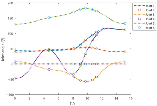
Figure 1.
Joint angle.
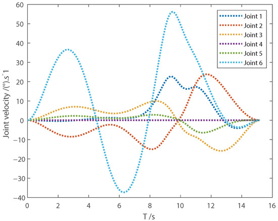
Figure 2.
Joint velocity.
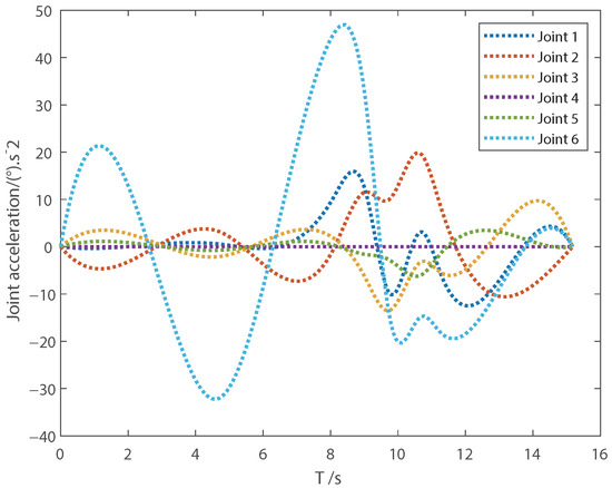
Figure 3.
Joint acceleration.
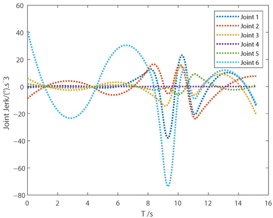
Figure 4.
Joint Jerk.
The multi-objective particle swarm optimization (MOPSO) algorithm is widely used in multi-objective optimization because of its fast convergence speed. Thus, in order to compare with the method proposed in this paper, we choose the MOPSO algorithm to solve the above optimal problem. Under the same conditions, we use the algorithm to obtain the optimal trajectory, and the results are shown in Figure 5, Figure 6, Figure 7 and Figure 8. Compared with Figure 1, Figure 2, Figure 3 and Figure 4, the execution time of the optimal trajectory obtained using the sequential quadratic programming method is significantly shorter than that obtained using MOPSO.

Figure 5.
Joint angle with MOPSO.
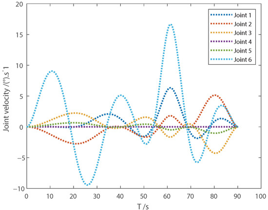
Figure 6.
Joint velocity with MOPSO.
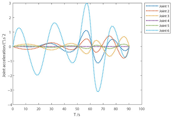
Figure 7.
Joint acceleration with MOPSO.
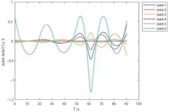
Figure 8.
Joint jerk with MOPSO.
6. Conclusions
In this paper, we proposed a manipulator trajectory planning method based on the seventh-order B-spline interpolation curve, which ensures that the joint velocity, acceleration and jerk are continuous. We transformed the motion constraint of the manipulator into the control vertex constraint of the trajectory curve, and used the sequential quadratic programming method to solve the time-optimal trajectory planning meeting the motion reduction bundle, obtaining the time-optimal jerk continuous trajectory. The simulation results verify the effectiveness of the proposed trajectory planning algorithm.
At present, we are building a 6-DOF robot experiment platform. In the future, we will apply the method proposed in this paper to the experimental platform, further improve the control strategy proposed in this paper to provide a practical and reliable control algorithm for 6-DOF robots, and greatly improve the operational efficiency of the robot arm.
Author Contributions
Conceptualization, Y.Z.; methodology, Y.Z. and G.H.; software, Z.H. and X.C.; validation, Y.Z., G.H., Z.W., Z.H. and X.C.; formal analysis, Y.Z. and G.H.; investigation, Z.H. and X.C.; resources, Y.Z.; writing—original draft preparation, Y.Z., G.H. and Z.W.; project administration, Y.Z.; funding acquisition, Y.Z. All authors have read and agreed to the published version of the manuscript.
Funding
This work is supported by (1) Hubei Province Technology Innovation Key Research and Development Project (No. 2023BAB071); (2) National Natural Science Foundation of China (No. 52205536); (3) Hubei Province Central Government Guide Local Science and Technology Development Project (No. 2022BGE035); and (4) Hubei Province Nature Science Foundation (No. 2023AFB380).
Institutional Review Board Statement
Not applicable.
Informed Consent Statement
Not applicable.
Data Availability Statement
Not applicable.
Conflicts of Interest
The authors declare no conflict of interest.
References
- Siliciano, B.; Sciavicco, L.; Villani, L.; Oriolo, G. Robotics: Modelling, Planning and Control; Springer: New York, NY, USA, 2010; pp. 415–418. [Google Scholar]
- Kohrt, C.; Stamp, R.; Pipe, A.; Kiely, J.; Schiedermeier, G. An online robot trajectory planning and programming support system for industrial use. Robot. Comput.-Integr. Manuf. 2013, 29, 71–79. [Google Scholar] [CrossRef]
- Madridano, A.; Al-Kaff, A.; Martín, D.; De La Escalera, A. Trajectory planning for multi-robot systems: Methods and applications. Expert Syst. Appl. 2021, 173, 114660. [Google Scholar] [CrossRef]
- Zhang, Y.; Sun, Z.; Sun, Q.; Wang, Y.; Li, X.; Yang, J. Time-jerk optimal trajectory planning of hydraulic robotic excavator. Adv. Mech. Eng. 2021, 13, 16878140211034611. [Google Scholar] [CrossRef]
- Wu, G.; Zhao, W.; Zhang, X. Optimum time-energy-jerk trajectory planning for serial robotic manipulators by reparameterized quintic NURBS curves. Proc. Inst. Mech. Eng. Part C J. Mech. Eng. Sci. 2021, 235, 4382–4393. [Google Scholar] [CrossRef]
- Zhou, J.; Cao, H.; Jiang, P.; Li, C.; Yi, H.; Liu, M. Energy-saving trajectory planning for robotic high-speed milling of sculptured surfaces. IEEE Trans. Autom. Sci. Eng. 2021, 19, 2278–2294. [Google Scholar] [CrossRef]
- Rubio, F.; Valero, F.; Sunẽr, J.L.S.; Mata, V. A comparison of algorithms for path planning of industrial robots. In Proceedings of the EUCOMES 08: The Second European Conference on Mechanism Science, Cassino, Italy, 17–20 September 2008; Springer: Berlin/Heidelberg, Germany, 2009; pp. 247–254. [Google Scholar]
- Valero, F.; Mata, V.; Besa, A. Trajectory planning in workspaces with obstacles taking into account the dynamic robot behaviour. Mech. Mach. Theory 2006, 41, 525–536. [Google Scholar] [CrossRef]
- Heo, H.J.; Son, Y.; Kim, J.M. A trapezoidal velocity profile generator for position control using a feedback strategy. Energies 2019, 12, 1222. [Google Scholar] [CrossRef]
- Wu, J.; Wang, D.; Wang, L. A control strategy of a two degrees-of-freedom heavy duty parallel manipulator. J. Dyn. Syst. Meas. Control 2015, 137, 061007. [Google Scholar] [CrossRef]
- Gasparetto, A.; Zanotto, V. Optimal trajectory planning for industrial robots. Adv. Eng. Softw. 2010, 41, 548–556. [Google Scholar] [CrossRef]
- Zanotto, V.; Gasparetto, A.; Lanzutti, A.; Boscariol, P.; Vidoni, R. Experimental validation of minimum time-jerk algorithms for industrial robots. J. Intell. Robot. Syst. 2011, 64, 197–219. [Google Scholar] [CrossRef]
- Gallant, A.; Gosselin, C. Extending the capabilities of robotic manipulators using trajectory optimization. Mech. Mach. Theory 2018, 121, 502–514. [Google Scholar] [CrossRef]
- Seki, H.; Tadakuma, S. Minimum jerk control of power assisting robot on human arm behavior characteristic. In Proceedings of the 2004 IEEE International Conference on Systems, Man and Cybernetics, The Hague, The Netherlands, 10–13 October 2004; Volume 1, pp. 722–727. [Google Scholar]
- Hermand, E.; Nguyen, T.W.; Hosseinzadeh, M.; Garone, E. Constrained control of UAVs in geofencing applications. In Proceedings of the 2018 26th Mediterranean Conference on Control and Automation (MED), Zadar, Croatia, 19–22 June 2018; pp. 217–222. [Google Scholar]
- Zhang, T.; Zhang, M.; Zou, Y. Time-optimal and smooth trajectory planning for robot manipulators. Int. J. Control. Autom. Syst. 2021, 19, 521–531. [Google Scholar] [CrossRef]
- Su, T.; Cheng, L.; Wang, Y.; Liang, X.; Zheng, J.; Zhang, H. Time-optimal trajectory planning for delta robot based on quintic pythagorean-hodograph curves. IEEE Access 2018, 6, 28530–28539. [Google Scholar] [CrossRef]
- Bureerat, S.; Pholdee, N.; Radpukdee, T.; Jaroenapibal, P. Self-adaptive MRPBIL-DE for 6D robot multiobjective trajectory planning. Expert Syst. Appl. 2019, 136, 133–144. [Google Scholar] [CrossRef]
- Raheem, F.A.; Sadiq, A.T.; Abbas, N.A.F. Robot arm free Cartesian space analysis for heuristic path planning enhancement. Int. J. Mech. Mechatron. Eng 2019, 19, 29–42. [Google Scholar]
- Gasparetto, A.; Boscariol, P.; Lanzutti, A.; Vidoni, R. Path planning and trajectory planning algorithms: A general overview. In Motion and Operation Planning of Robotic Systems: Background and Practical Approaches; Springer: Berlin/Heidelberg, Germany, 2015; pp. 3–27. [Google Scholar]
- Liu, L.; Yao, W.; Guo, Y. Prescribed performance tracking control of a free-flying flexible-joint space robot with disturbances under input saturation. J. Frankl. Inst. 2021, 358, 4571–4601. [Google Scholar] [CrossRef]
- Geisslinger, M.; Poszler, F.; Lienkamp, M. An ethical trajectory planning algorithm for autonomous vehicles. Nat. Mach. Intell. 2023, 5, 137–144. [Google Scholar] [CrossRef]
- He, S.; Hu, C.; Lin, S.; Zhu, Y. An online time-optimal trajectory planning method for constrained multi-axis trajectory with guaranteed feasibility. IEEE Robot. Autom. Lett. 2022, 7, 7375–7382. [Google Scholar] [CrossRef]
- Yu, X.; Dong, M.; Yin, W. Time-optimal trajectory planning of manipulator with simultaneously searching the optimal path. Comput. Commun. 2022, 181, 446–453. [Google Scholar] [CrossRef]
- Huang, P.; Xu, Y.; Liang, B. Global minimum-jerk trajectory planning of space manipulator. Int. J. Control. Autom. Syst. 2006, 4, 405–413. [Google Scholar]
- Lin, C.; Chang, P.; Luh, J. Formulation and optimization of cubic polynomial joint trajectories for industrial robots. IEEE Trans. Autom. Control 1983, 28, 1066–1074. [Google Scholar] [CrossRef]
- Bazaz, S.A.; Tondu, B. Minimum time on-line joint trajectory generator based on low order spline method for industrial manipulators. Robot. Auton. Syst. 1999, 29, 257–268. [Google Scholar] [CrossRef]
- Gasparetto, A.; Lanzutti, A.; Vidoni, R.; Zanotto, V. Experimental validation and comparative analysis of optimal time-jerk algorithms for trajectory planning. Robot. Comput.-Integr. Manuf. 2012, 28, 164–181. [Google Scholar] [CrossRef]
- Fang, S.; Ma, X.; Zhao, Y.; Zhang, Q.; Li, Y. Trajectory planning for seven-DOF robotic arm based on quintic polynormial. In Proceedings of the International Conference on Intelligent Human-Machine Systems and Cybernetics (IHMSC), Hangzhou, China, 24–25 August 2019; Volume 2, pp. 198–201. [Google Scholar]
- Kucuk, S. Optimal trajectory generation algorithm for serial and parallel manipulators. Robot. Comput.-Integr. Manuf. 2017, 48, 219–232. [Google Scholar] [CrossRef]
- Gasparetto, A.; Zanotto, V. A new method for smooth trajectory planning of robot manipulators. Mech. Mach. Theory 2007, 42, 455–471. [Google Scholar] [CrossRef]
- Freeman, P. Minimum Jerk Trajectory Planning for Trajectory Constrained Redundant Robots; Washington University in St. Louis: St. Louis, MO, USA, 2012. [Google Scholar]
- Tan, G.; Wang, Y. Theoretical and experimental research on time-optimal trajectory planning and control of industrial robots. Control Theory Appl. 2003, 20, 185–192. [Google Scholar]
Disclaimer/Publisher’s Note: The statements, opinions and data contained in all publications are solely those of the individual author(s) and contributor(s) and not of MDPI and/or the editor(s). MDPI and/or the editor(s) disclaim responsibility for any injury to people or property resulting from any ideas, methods, instructions or products referred to in the content. |
© 2023 by the authors. Licensee MDPI, Basel, Switzerland. This article is an open access article distributed under the terms and conditions of the Creative Commons Attribution (CC BY) license (https://creativecommons.org/licenses/by/4.0/).