A Ground-Risk-Map-Based Path-Planning Algorithm for UAVs in an Urban Environment with Beetle Swarm Optimization

Abstract

This paper presents a path-planning strategy for unmanned aerial vehicles (UAVs) in urban environments with a ground risk map. The aim is to generate a UAV path that minimizes the ground risk as well as the flying cost, enforcing safety and efficiency over inhabited areas. A quantitative model is proposed to evaluate the ground risk, which is then used as a risk constraint for UAV path optimization. Subsequently, beetle swarm optimization (BSO) is proposed based on a beetle antennae search (BAS) that considers turning angles and path length. In this proposed BSO, an adaptive step size for every beetle and a random proportionality coefficient mechanism are designed to improve the deficiencies of the local optimum and slow convergence. Furthermore, a global optimum attraction operator is established to share the social information in a swarm to lead to the global best position in the search space. Experiments were performed and compared with particle swarm optimization (PSO), genetic algorithm (GA), firefly algorithm (FA), and BAS. This case study shows that the proposed BSO works well with different swarm sizes, beetle dimensions, and iterations. It outperforms the aforementioned methods not only in terms of efficiency but also in terms of accuracy. The simulation results confirm the suitability of the proposed BSO approach.

1. Introduction

Unmanned aerial vehicles (UAVs) have gained significant momentum in recent years, and their extensive uses have induced rapid growth in related research areas [1,2,3]. Currently, UAVs are used in a wide range of applications, both in civil and military fields. In particular, the use of UAVs in urban environments will increase significantly in the near future, forming the core component of urban air mobility (UAM), as described in smart cities [4,5,6]. For this reason, it will be mandatory to enhance the safety of flight operations, especially in urban inhabited areas with the lowest flying costs.

However, the increase in UAV operations in urban low-altitude airspace will inevitably lead to a high likelihood of crashes on the ground because of unexpected UAV accidents in the air, which pose significant risks to people on the ground. Therefore, how to plan an optimal flying path for UAVs with the lowest ground risk and flying cost possible is an important and indispensable problem in UAM.

Path planning is a key element in providing autonomy to UAVs in the execution of UAM missions by defining a set of waypoints to reach a destination while satisfying some optimality criteria and minimizing risk for people on the ground. The topic has been widely studied, and a large number of methods have been proposed. One popular family of path-planning methods includes sample-based techniques, which are used to explore the search space through a sampling scheme. Widely diffused approaches include probabilistic roadmaps (PRM) [7,8], rapidly exploring random trees (RRT) [9,10], and other RRT-based methods [11,12]. Another popular kind of path-planning algorithm is based on graph-searching algorithms, which usually include the Voronoi diagram searching method [13], the Dijkstra algorithm [14], and the A* algorithm [15]. All of these methods use Eppstein’s k-best algorithm to find the optimal UAV path. The third group of optimization techniques, which are also called population-based evolutionary algorithms, are now widely accepted and used to solve the UAV path-planning problem, including particle swarm optimization (PSO) [16,17], genetic algorithm (GA) [18,19], firefly algorithm (FA) [20,21], beetle antennae search (BAS) [22,23], and related improved methods [24,25]. When using graph-searching-based algorithms, such as the Dijkstra algorithm, their expansion in every direction and blind recalculation of each direction is computationally expensive. Additionally, the Dijkstra algorithm cannot handle negative transition costs, which means that the calculated path is not necessarily the shortest. For the A* algorithm, the memory requirements are high because the algorithm needs to save the complete list of open nodes, which makes the space for memory limited. In this way, the use of heuristic algorithms is becoming an effective and popular way to optimize UAV path planning in complicated situations with high efficiency and accuracy, and only a few parameters are needed.

Currently, it is difficult for these UAV path-planning algorithms to take ground risk distributions into account, which leads to unsafe operations for people on the ground. The risk caused by UAV operations in UAM is difficult to quantify. Therefore, some research has been conducted in an attempt to solve this problem with qualitative methods instead. For example, Primatesta S. et al. [26] proposed two algorithms for UAV path planning based on risk awareness to tackle dynamic risks and threats within UAVs’ operational environments. The authors also studied the possible risk factors in UAM for UAV operations [5]. Campbell D. et al. [27] proposed a 4D path-planning method for UAVs based on the risk–cost map to enable UAVs to fly along a cost-effective path. However, all the proposed algorithms only focus on UAV operation rules qualitatively instead of modeling the risk events related to urban characteristics. Some other researchers have studied city obstacles, weather conditions, and other vehicles on the ground, which are taken as possible threats [28,29].

In this paper, a beetle swarm optimization (BSO)-based path-planning algorithm for UAVs in urban environments is proposed. The ground risk distribution is considered as an input for this optimization model. First, a quantitative mechanism was designed to evaluate the effects of ground risk on a generated UAV path. Next, the turning angles and path length were incorporated as constraint conditions for the proposed BSO model. Subsequently, an adaptive step-size mechanism for each beetle and a random proportionality coefficient were designed to improve the deficiencies of the slow convergence and local optimum, which usually appear in standard BASs. Finally, a global optimum attraction operator was established for all the beetles to share social information in the whole beetle swarm in order to lead each individual towards the global best position in the search space. In comparison with PSO, GA, FA, and standard BAS, the proposed BSO method worked well under all the scenarios with different swarm sizes, individual dimensions, and iterations. Simulation results confirmed the suitability of the proposed approach.

The remainder of this paper is organized as follows: The description of the problem is provided in Section 2. A detailed model and the methodology are provided in Section 3. Section 4 describes the proposed BSO-based path-planning algorithm for UAVs in urban areas. A case study and algorithm validations can be found in Section 5. Finally, the paper is concluded in Section 6.

2. Problem Description

In this paper, the objective of a path-planning algorithm is to generate an optimum route based on a given risk map of the flying area, which should also be suitable for all the UAVs to follow and with the lowest possible flying cost. As shown in Figure 1, a risk map is provided in the form of grids. The size of this ground risk map is 30 km × 20 km. The different colors of the grids show different risk levels of the ground areas, whose total number is 600. The grids with higher risk levels should not be in the way of the UAV’s operation, which means that the ground areas with higher risk should be avoided in the UAV’s route. In this way, determining a path from a given starting point S to a destination point D with the lowest risk as well as the lowest flying cost becomes a key problem.

As illustrated in Figure 1, a complete UAV flying path can be composed of many waypoints. For example, there are seven waypoints in total in this figure, which are WP₁, WP₂, WP₃, WP₄, WP₅, WP₆, and WP₇. By using these seven waypoints, a flying path for UAVs can be formulated. The number of waypoints is variable and can be set differently based on the UAV’s operation scenario. Therefore, determining the positions of waypoints with the lowest flying cost as well as the lowest ground risk becomes the target of a path-planning algorithm. Meanwhile, a generated UAV route should be guaranteed to be smooth enough for UAVs to follow.

According to the analysis above, a ground risk map would be set as an input for the path-planning model in the proposed BSO method. It is assumed that the ground risk map can be provided in advance, which will be used directly as a constraint condition to make the overall risk level of a flying path as low as possible. Besides the ground risk, some other factors are taken into account, including the requirements of UAVs themselves, as shown in Figure 2. In this paper, the most basic method is to generate collision-free paths in two-dimensional environments with the lowest path risk. It is known that the complexity analysis is quite important, which can predict the execution time of the algorithm as a function of the problem’s input size. In the proposed path-planning algorithm, the input size mainly consists of two variables, which represent the complexity of the UAVs and low-altitude airspace, respectively. In this condition, the complexity of a UAV path-planning algorithm would increase significantly compared with the traditional path-planning problems. Usually, the spatial pose of a UAV or its configuration is uniquely defined by its degrees of freedom. Correspondingly, the degrees of freedom of UAVs have possibly become the most crucial parameter in determining the complexity of the path-planning problem. So, the diverse range of air-borne movements a UAV may utilize in the airspace introduces an exponential growth in the potential paths available, which further presents significant complexity. In order to reduce the complexity, some assumptions are made in the proposed model. It is generally accepted that all the UAVs are assumed to be some mass points, ideally, in which condition elevation levels and taking off/landing trajectories are reasonably neglected. Based on the analysis and calculations, the time complexity level would be above O(n²). Figure 2 gives the overall framework of the proposed method. Firstly, when the UAVs are following a determined flying path, the turning angles between any two sequential waypoints should satisfy their operation limits. Subsequently, the length of a generated path should be as short as possible to reduce energy consumption and extend the UAV’s lifetime further. As a result, the path risk constraint, path turn constraint, and path length constraint are included in the proposed path-planning model, which is shown in Figure 2.

3. Model and Methodology

In this section, the proposed UAV path-planning model and objective function design are provided, respectively. How to present a UAV path is described first. Based on this defined path presentation, three constraint conditions for a UAV’s flying path are modeled and quantized. Finally, the objective function for the proposed BSO method is established by incorporating their weight coefficients.

3.1. Path Presentation

A UAV path can be denoted as a sequence of waypoints, which is shown in Figure 3. In this figure, there is a possible path between the starting point S and destination point D, which can be expressed as a waypoint set WP = {WP₁, WP₂, WP₃, WP₄, WP₅, WP₆, WP₇}. The size of WP is seven, as shown in Figure 3, which is a variable based on different flying requirements. In order to obtain the accurate coordinates of all the seven waypoints as well as to simplify the calculation, N vertical lines are made to x-Axis passing each waypoint WP_i (i = 1, 2, …, 7), all of which are parallel to y-Axis and are denoted as a vertical line set L = {L₁, L₂, L₃, L₄, L₅, L₆, L₇}. Both the waypoint set WP and the vertical line set L share the same size N (N = 7). It is obvious that the size N can be quite different based on different scenarios. Without loss of generality, the distance d between every two neighboring lines in the vertical line set L will be kept the same. It is assumed that the distance between vertical line L_S and L₁ and the distance between vertical line L₇ and L_D are also set as the same value d. As a result, this accurate value of the distance d can be calculated easily under the condition that the size of the two used sets and the coordinates of the starting point S and destination point D are provided.

It is supposed that the coordinate of a waypoint WP_i can be expressed as (x_i, y_i) and i = 1, 2, …, N. The specified positions of the starting and destination points S and D can be given as (x_S, y_S) and (x_D, y_D), respectively. In this way, the abscissa of any waypoint i in the waypoint set WP can be determined by using Equation (1). N is the total number of waypoints on the path.

$$x_i=x_S+i\cdot \frac{x_D-x_S}{N+1}$$

(1)

Once the abscissae of all the waypoints in the set WP are determined by using Equation (1), calculating the global optimum vertical coordinates of all the N waypoints becomes the objective of a path-planning algorithm.

3.2. Path Risk Constraint

When UAVs are operating in urban airspace, there is a chance of failure, which leads to the possibility of hitting people on the ground and may cause fatalities. In this way, for a planned UAV path, the risk imposed on people on the ground should be as low as possible, especially when a ground risk map is provided in advance. To guarantee the safety of ground people, the risk caused by the UAV’s operation route should be quantized in the planning model first. As shown in Figure 4, there is a potential UAV path, which is expressed as a red line. This potential path would go through different risk grids on the ground, resulting in different risk levels. The size of each grid on the ground is 1 km × 1 km, which is the same as described in Figure 1. In Figure 4, R_i,j means the risk value of each grid G_i,j. It is supposed that these values can be determined and given by the existing risk estimation methods [30], which are considered to be used directly.

In order to quantize the risk caused by the planned UAV path, a path box is defined in each risk grid where the UAV path goes through, as described in Figure 4. The path boxes are denoted as a number of red rectangles with dash lines. A path box covers the complete UAV path segment in a risk grid on the ground. As shown in the example in Figure 4, the total number of the path boxes is 9, which can be denoted as B_k (k = 1, 2, …, 9). Suppose the length of a UAV path segment in a path box B_k is denoted as L_Bk (k = 1, 2, …, 9). Actually, the accurate length of a path segment in a path box can be calculated easily once the UAV path is generated. Correspondingly, the risk of a path segment in each path box can be obtained by multiplying the length of a path segment and the risk of a specified path box. As a result, the total path risk constraint can be mathematically quantized using Equation (2) by adding the risk values of all the path segments in all the path boxes.

$$J_R={\displaystyle \sum _{k=1}^N{R}_{Bk}\cdot L_{Bk}}$$

(2)

In Equation (2), J_R is the quantized risk constraint, R_Bk is the grid risk value in which a path box B_k is located, L_Bk is the length of a path segment divided by a path box B_k, and N is the number of path boxes on the whole UAV path.

3.3. Path Turn Constraint

When UAVs are operating in low-altitude airspace over inhabited urban areas, all the turning angles should be subject to limitations of the UAVs’ performances, which means that the planned path should be suitable enough to follow. For example, once a turning angle is out of the scope of UAVs’ limitation, they cannot follow the path, which proves that it is not an optimal solution for the path optimization problem. According to this requirement, the path should be evaluated by using path turn constraint. Therefore, it needs to be quantized for a more accurate optimization. Figure 5 shows the quantization of the path turn constraint for a UAV path. As previously analyzed, the flying path is composed of several waypoints, and each of them can be denoted as WP_i. The coordinate of a waypoint WP_i on a two-dimensional plane can be denoted as (WP_i _x, WP_i _y).

In the proposed model, the turning angle is defined as the deflection between two sequential waypoints, such as WP_i and WP_i+1 in Figure 5. In order to obtain a preferred UAV flight path that is as close to the straight line connecting the starting point with the destination point as possible, a deflection angle between the line connecting two sequential waypoints and the horizontal line passing the previous waypoint is used as the turning angle. In Figure 5, a_i is the defined turning angle between two neighboring waypoints, WP_i and WP_i+1, which is assumed to be positive all the time. Its value can be calculated by using the 2D coordinates of two sequential waypoints, as expressed in Equation (3). In this equation, the turning angle a_i is denoted by the arctangent and would be kept positive from the beginning to the end in the proposed model. (WP_i _x, WP_i _y) and (WP_i+1 _x, WP_i+1 _y) are the two coordinates of waypoints WP_i and WP_i+1, respectively. The accurate turning angle at each waypoint on a path can be calculated by using Equation (3).

$${\alpha }_i=\arctan \left|\frac{W{P}_{i+1}\_y-W{P}_i\_y}{W{P}_{i+1}\_x-W{P}_i\_x}\right|$$

(3)

Once the turning angle at every waypoint is obtained by using Equation (3), the total path turn constraint can then be quantized with Equation (4), which is denoted as J_T. In this equation, N is the number of waypoints on a UAV path, which is determined by the path-planning algorithm.

$$J_T={\displaystyle \sum _{i=1}^N{\alpha }_i}$$

(4)

3.4. Path Length Constraint

When UAVs are flying from a specified starting point S to a destination point D, as in the scenario described in Figure 1, the distance should be guaranteed to be as short as possible to minimize UAV energy consumption and further prolong the battery life. Thus, the objective becomes how to obtain an optimal path, namely in terms of the shortest one. In order to realize this objective, the path length needs to be one of the constraints in the proposed optimization model.

Considering an actual operation scenario, to simplify the path-planning model, the mileage during the UAVs’ turns on a path is ignored, and only the straight-line distances between sequential waypoints are taken into account. Based on this hypothesis, the length of a UAV path can be defined as the sum of all the path segments between any two neighboring waypoints. According to Figure 5, the length of a UAV path is the sum of the straight-line distances between any two waypoints WP_i and WP_i+1, which is denoted as Len_i. In this way, the value of Len_i can be obtained using Equation (5). In this equation, (WP_i _x, WP_i _y) and (WP_i+1 _x, WP_i+1 _y) are the two-dimensional coordinates of the waypoints WP_i and WP_i+1 on a generated path.

$$Le{n}_i=\sqrt{{\left(W{P}_{i+1}\_x-W{P}_i\_x\right)}^2+{\left(W{P}_{i+1}\_y-W{P}_i\_y\right)}^2}$$

(5)

The path length constraint can be quantized by the sum of all the path segments, which is given in Equation (6). N is the number of all the waypoints on a generated UAV path.

$$J_L={\displaystyle \sum _{i=1}^{N}Le{n}_i}$$

(6)

3.5. Objective Function Design

Based on Equations (2), (4), and (6), the objective function for the proposed BSO-based path-planning algorithm can be formulated, which is given in Equation (7). In this equation, w₁, w₂, and w₃ are the three weight coefficients that are used to evaluate the effects of the ground risk, turning angle, and path length. They should be subject to UAV’s performances, including the maximum turning angles and the maximum flying distances, all of which are determined once they are manufactured. Only in this way will the path generated by the path-planning algorithms be suitable and followed by UAVs, which makes it practical and significant.

$$\begin{array}{l}J=\mathrm{minimize}\left\{{\omega }_1\cdot J_R+{\omega }_2\cdot J_T+{\omega }_3\cdot J_L\right\}\\ \hspace{1em}\mathrm{subject}\hspace{1em}\mathrm{to}\hspace{1em}\mathrm{UAV}’\mathrm{s}\hspace{1em}\mathrm{performaces}\end{array}$$

(7)

Concerning the obtained Equation (7), locating the optimum solutions, which would make the total cost J the minimum, becomes a core mission of the proposed path-planning algorithm in the next section.

4. Beetle Swarm Optimization (BSO) Method

In this section, first, the standard beetle antennae search (BAS) algorithm is briefly introduced. Next, the beetle swarm optimization (BSO) method is proposed in detail. Finally, how the proposed BSO method can be realized is given.

4.1. Standard Beetle Antennae Search (BAS) Algorithm

The standard beetle antennae search (BAS) algorithm belongs to a kind of heuristic optimization technique that runs with a high efficiency and a low complexity by simulating the beetle’s movement to find the food in nature step by step, which is quite similar to the particle swarm optimization (PSO), genetic algorithm (GA), and firefly algorithm (FA). After several rounds of moves, the beetle in BAS can locate the global optimum solutions for a very complicated problem. This is now widely used in optimization fields.

There are two main stages in the current standard BAS algorithm. The first is the search stage, and the other is the detection stage. There is only one beetle in the standard BAS. Every time this beetle moves in a random direction, it is correspondingly defined as the search stage. Subsequently, in order to simulate the randomness of this beetle’s movement in the search stage, a random unit vector $\overrightarrow{b}\in R^N$ is formulated to describe the beetle’s random moving direction. With this assumption, the position coordinates of this beetle’s right antennae and left antennae in the search space, which are denoted as x_R and x_L, respectively, can be calculated using Equation (8).

$$\left\{\begin{array}{l}{x}_R=x^k-\frac{d_0}{2}\cdot \overrightarrow{b}\\ x_L=x^k+\frac{d_0}{2}\cdot \overrightarrow{b}\end{array}\right.$$

(8)

In Equation (8), k means the kth move of the beetle during the search process. x^k is the centroid of the beetle’s current position in the kth move. d₀ is the distance between the beetle’s right antennae and the left antennae, which also represents the beetle’s search area. The value of d₀ is only decided by the size of the beetle; namely, a bigger beetle means a larger d₀. Actually, it highly depends on the scale of a specific optimization problem.

Once the beetle’s search stage is finished, the detection stage starts, which can be performed using Equation (9). There is no doubt that the position of the kth move is related to (k−1)th position. Step^k is the step size in the kth move, which could be set as a constant or a variable. sign(x) is a sign function which can only give two results, namely 1 and −1. The value of 1 or −1 is only determined by the plus or minus of the independent variable x.

$$x^k=x^{k-1}-Ste{p}^k\cdot \overrightarrow{b}\cdot sign(f(x_L)-f(x_R))$$

(9)

f(x) is a defined cost function that can also be set as the objective function. Only the beetle positions introduce less cost that can be saved during each move. f(x_R) and f(x_L) are the cost of the right antennae and left antennae, respectively. Repeatedly, by several moves, the optimum positions with the least cost can be finally obtained.

However, the convergence of the standard BAS is highly dependent on the beetle’s random direction in every move, which can easily lead to a local optimum instead of the global best solutions. Also, the step size of the beetle’s move cannot guarantee that the current objective value is better than the previous one in the iterative process.

4.2. Beetle Swarm Optimization (BSO) Method

In order to overcome the drawbacks of the standard BAS, a beetle-swarm-based optimization (BSO) is proposed, which takes the ground risk distribution into account. It is assumed that the size of a beetle swarm is M, which means that the number of beetles is M. Subsequently, an adaptive step size for each beetle is presented to guarantee the diversity of this constructed beetle swarm. A proportionality coefficient is also designed as a random variable for each beetle’s movement to keep the flexibility. In the end, a kind of optimum attraction operator is built to help enforce the effects of the social information on all the beetles’ behaviors.

(1)

Adaptive step size for each beetle

The step sizes of the beetles could determine the distances of their moves in every iteration, which correspondingly lead to different optimization accuracies and efficiencies. For any beetle i in a swarm in the kth move, the step size denoted as Step_i^k can be calculated by using Equation (10), which is an adaptive parameter as the beetle moves. Specifically, in this equation, Step_i^k−1 is the step size of beetle i in the (k−1)th move. c_i is a constant that would be unequal for the different beetles even though they belong to the same beetle swarm. Normally, c_i is set as a positive value, which is smaller than one. Rand_i^k is used to generate a random value between 0 and 1 to guarantee the randomness of the beetle’s step size. By using Equation (10), an adaptive step size can be generated for every beetle i in each move k.

$$Ste{p}_i^k=Ste{p}_i^{k-1}\cdot \left[c_i+Ran{d}_i^k\times 0.1\right]$$

(10)

In this way, by introducing this kind of randomness into the step size for every beetle adaptively, the deficiency of the local optimum solutions could be avoided to some extent. Also, the step size is highly related to the number of iterations. As shown in Equation (10), it is obvious that in the last few iterations, the step size is much smaller compared with that in the few beginning iterations, which could further make the expected optimum solutions easy to find. This adoption of an adaptive step size in the proposed BSO method guarantees that all the beetles would move to the global optimum positions in a short time with a high accuracy, which makes the algorithm more efficient even in a complicated situation with a large number of beetles existing in a swarm.

(2)

Random proportionality coefficient

It is known that a bigger beetle moves further in terms of distance every iteration, which means that there is a proportionality coefficient between the beetle size and its step size. As illustrated in Equation (8), a predefined distance d₀ does exist between the beetle’s right and left antennas to describe the sizes of the beetles exactly. A larger d₀ means a larger beetle. In the standard BAS algorithm, this proportionality coefficient is set as a constant, which, in turn, could reduce the complexity of the BAS. However, on the contrary, using a constant proportionality coefficient would make it difficult for the beetles to reach the global optimum positions, leading to a lot of swings during the optimization. In this way, the solutions obtained by the standard BAS algorithm may not be the optimum, and possibly, it would be suboptimal around the optimum positions.

In the proposed BSO method, a random proportionality coefficient is designed to improve the suboptimal problem that appears in the standard BAS algorithm. For a beetle i in the kth move, a random proportionality coefficient can be denoted as R_i^k, which is calculated with Equation (11). In this equation, e₁ⁱ and e₂ⁱ are two constants for a beetle i to limit the scope of proportionality coefficient R_i^k during each move. Generally, e₁ⁱ is larger than e₂ⁱ for a beetle i. Also, these two parameters, e₁ⁱ and e₂ⁱ, can be different for different beetles. Furthermore, Rand_i^k is used to generate a random value between 0 and 1 in order to guarantee the randomness that is needed in the proportionality coefficient.

$$R_i^k=e_1^i+Ran{d}_i^k\times e_2^i$$

(11)

Once a random proportionality coefficient R_i^k is generated, the relationship of the distance d₀^i,k between a beetle i’s right antennae and left antennae, and the step size Step_i^k of beetle i in the kth move, can be determined correspondingly. It can be expressed as d₀^i,k = Step_i^k/R_i^k directly. In this situation, by changing the sizes of beetles themselves dynamically or, to be more precise, according to the introduced random proportionality coefficient, the suboptimal problem in the standard BAS could be solved and avoided greatly.

(3)

Optimum attraction operator

In the standard BAS algorithm, there is only one beetle that moves as it tries to find the global optimum solutions. However, in the proposed BSO method, there are M beetles in a given swarm. During the moves of all the beetles, the current global optimum solution would attract other beetles to approach step by step. To address this attraction, an optimum attraction operator is designed to generate a force attracting every beetle to move towards the global best position in the search space. The global knowledge of the swarm is used to help locate a global optimum solution, which can also be called social knowledge. As shown in Equation (12), A_F is defined as an optimum attraction operator, which could build the connections between the global best position G_C and other non-global best individuals. In each iteration, the optimum attraction operator A_F would generate a kind of attractive force to make beetles get closer and closer to the global optimum solutions. In this way, the proposed BSO method can locate the optimum position efficiently and accurately by using social knowledge.

$$x_i^k=x_i^{k-1}+A_F\cdot (G_C-x_i^{k-1})-Ste{p}_i^k\cdot \overrightarrow{b}\cdot sign(f(x_L)-f(x_R))$$

(12)

Equation (12) also shows how the position of a beetle’s i in the current kth iteration updates. It considers the effects of the current global best in the beetle swarm as well as the beetle’s own position in the (k−1)th move. From Equation (12), it can be seen that both the proposed adaptive step size and random proportionality coefficient are included for the beetle position update, which makes the optimization more accurate and efficient. Therefore, by combining the positive effects from a beetle swarm with the individual effects of beetles, both the accuracy and the efficiency of the proposed BSO method are better improved than the standard BAS algorithm.

4.3. Realization of the Proposed BSO

Based on the analysis above, the detailed realization of the proposed BSO method can be described as follows: The flowchart is provided in Figure 6. From this figure, we can see that there are four steps, which are the scene construction, algorithm initialization, determination of beetle sizes, updates of the beetles’ positions, and global optimum positions. The illustrations for every step can be found, and the pseudocode is provided in Figure 7.

• Step 1: Scene construction.

The coordinates of the starting and destination points for UAVs to operate are given first as S and D. The positions of S and D should be in the scope, which is covered by the ground risk map, as shown in Figure 1. After that, a beetle swarm would be generated with the determined number of beetles M. All the beetles’ dimensions are set as the same as N. The positions of all the beetles are the possible waypoint sets for UAVs. N is also the number of the waypoints between the starting point S and the destination point D; namely, the size of each waypoint set is N.

• Step 2: Algorithm initialization.

In the proposed BSO method, the total number of all the beetles’ moves in a given swarm is initialized as T. In this way, there are T iterations to evolve for the optimization process. The move counter k starts from zero. The initial path cost is calculated by using Equation (7) based on all the beetles’ initial positions by incorporating the three main constraint conditions, including the ground risk, the turning angle, and the path length. The beetle with the lowest path cost would be saved and then selected as the current global best solution from the beginning to the current iteration.

• Step 3: Determination of beetle size.

First, set the beetle move counter k = k + 1. After that, for any beetle i in the current move k, the proposed adaptive step size Step_i^k and random proportionality coefficient R_i^k can be determined by using the two previously provided Equations (10) and (11), respectively. Once these two key parameters for the proposed BSO method are determined, the required distance d₀^i,k between the beetle i’s right and left antennas in the current kth move can be calculated with the equation d₀^i,k = Step_ik/R_i^k. In this way, the size of the current beetle i can be obtained finally.

• Step 4: Update the beetles’ positions and global best.

Once the sizes of all the beetles in a specified swarm are obtained, the estimated coordinates of the beetle i’s right and left antennas in the kth move can be calculated by using Equation (13), which can be further denoted as x_R^i,k and x_L^i,k, respectively. The corresponding cost of the beetle i’s right and left antennas in the kth move would be f(x_R^i,k) and f(x_L^i,k) under the condition of Equation (7). Based on the cost values of the right and left antennas, this beetle i’s position in the kth move would be updated with Equation (12). The current global best cost G_C could then be updated based on the latest beetle’s positions using Equation (7).

$$\left\{\begin{array}{l}{x}_R^{i,k}=x_i^{k-1}-\frac{d_0^{i,k-1}}{2}\cdot \overrightarrow{b}\\ x_L^{i,k}=x_i^{k-1}+\frac{d_0^{i,k-1}}{2}\cdot \overrightarrow{b}\end{array}\right.$$

(13)

• Step 5: Output of global best solution.

First, check whether the given termination condition T is satisfied or not; if not, go to Step 3 for the next iteration again. If it is satisfied, which means the beetle move counter k is larger than T, the beetle positions with the least path cost combined with the current global best cost G_C in the last beetle move would be the desired output. The obtained output is the global best solution in the search space, which would then be used as the UAV’s final waypoints.

According to the flowchart and the pseudocode provided in Figure 6 and Figure 7, only a few steps are needed to locate the global best solution for the UAV path-planning problem, which makes the proposed BSO method more efficient and practical.

5. Case Study and Algorithm Validation

In this section, a case study and algorithm validation are performed to prove the effectiveness of the proposed BSO method. All of the models and algorithms are coded in MATLAB and run on a server with a 2.8 GHz CPU and 16.0 GB of RAM.

5.1. Scenario and Parameter Settings

It is assumed that the UAV operation area is two-dimensional, with a size of 30 km × 20 km, as shown in Figure 1. The size of every ground grid is defined as 1 km × 1 km. The accurate risk value of each grid on the ground is provided in advance and is presented in the form of a thermodynamic chart. The coordinates of the given starting point S and destination point D are (0.5, 0.5) km and (28, 18) km, respectively. They are kept the same in the simulation. In this way, the mission of a path-planning algorithm is to generate an optimum flying route from S to D, which should also be suitable for UAVs to follow with the lowest flying cost. Meanwhile, the risk of a generated UAV path should be guaranteed to be as low as possible to prevent people from being hit by UAVs when they crash. Some other factors should be considered, which include the turning angles of the UAVs and the length of the path from S to D.

The effects of the swarm sizes, the individual dimensions, and the number of iterations on a planned UAV path are explored and compared. The detailed scenario parameter settings can be found in

Table 1. Scenario and parameter settings.

Item	Values
Scenario size	30 km × 20 km
Starting point	(0.5, 0.5) km
Destination point	(28, 18) km
Effects of swarm sizes	10, 20, 80, 90
Effects of individual dimensions	15, 20, 25, 30
Effects of iterations	50, 150, 250, 350

.

As illustrated in Table 1, three typical operation scenarios are considered to validate the proposed BSO method, namely Scenario 1, Scenario 2, and Scenario 3. These three scenarios would be used to test the effects of the different swarm sizes, different individual dimensions, and different numbers of iterations. Meanwhile, the smoothness of a generated UAV path is another important index to evaluate the performances of the path-planning algorithms. The smoother the path is, the easier it is for the UAVs to follow, which is more desirable. The path cost, path risk, path length, and turning angle are the four quantitative indexes to better validate the superiority of the proposed BSO method. Comparisons are made with some other heuristic algorithms based on these indexes, including PSO, GA, FA, and standard BAS.

5.2. Effects of Swarm Sizes

To explore the effects of the different swarm sizes on the proposed BSO method, the other two core parameters, including the dimension of each individual and the number of iterations, are set as 15 and 100, respectively. The normalized path risk, turning angle, path length, and total cost are selected as indicators to evaluate the algorithm’s performance. The generated UAV paths in a given 2D environment are also provided. Comparisons are made with PSO, GA, FA, and standard BAS algorithms.

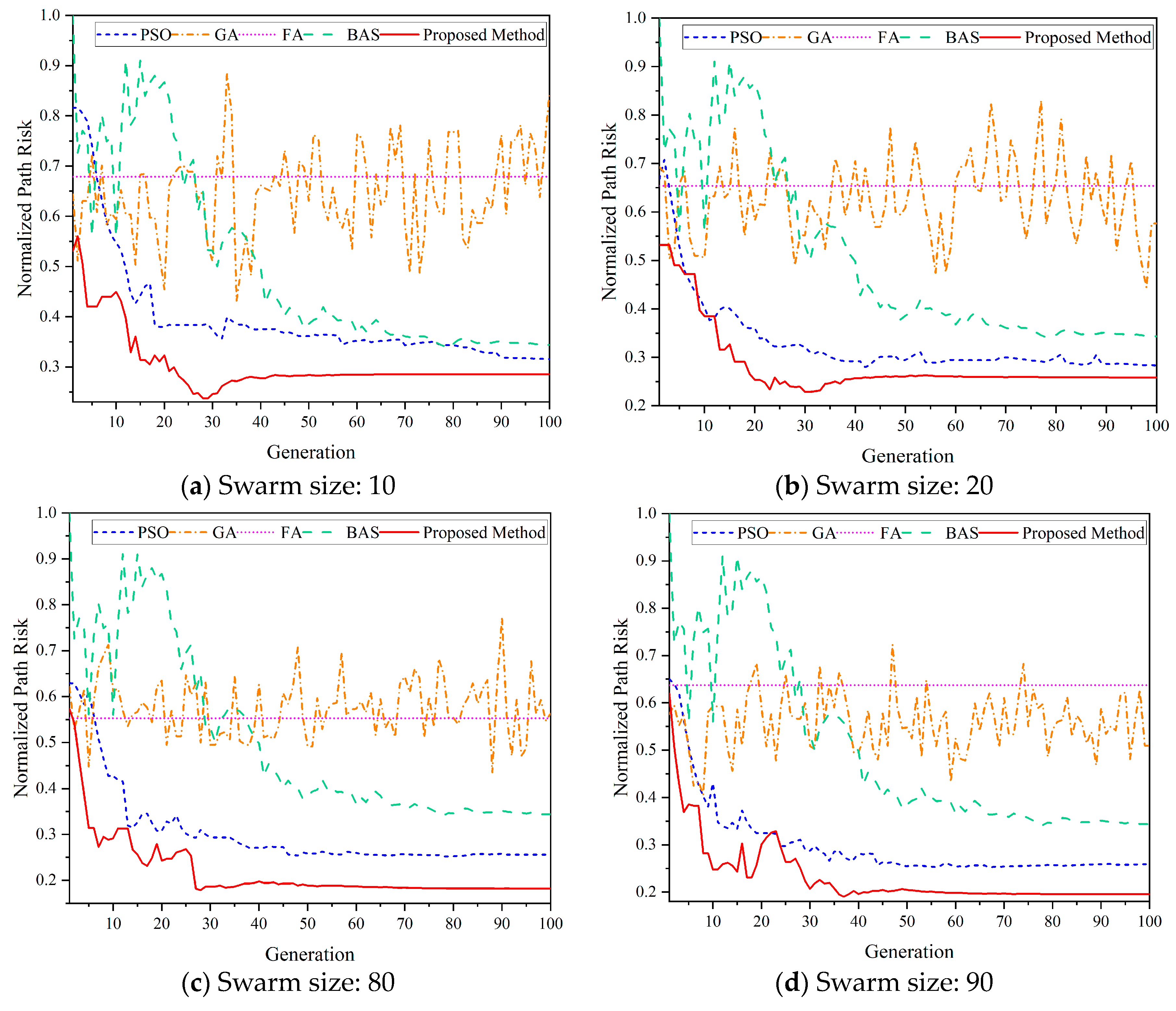
Figure 8 shows the effects of the swarm sizes on the UAV path risk. The numbers of the individuals in a swarm are set as 10, 20, 80, and 90. Comparisons are made with the other four existing methods, including PSO, GA, FA, and standard BAS. It should be noted that there is only one beetle in standard BAS. As a result, it cannot be affected by the swarm size. As shown in Figure 8, GA fluctuates the most from the first iteration to the end, regardless of how many individuals exist. For GA, it is difficult to locate the global optimum solutions in the search space. However, for FA, it is a straight line from the beginning to the end. It means the risk of a generated UAV path is the same, which illustrates that FA falls into a local optimum in this scenario. Oppositely, standard BAS, PSO, and the proposed BSO method could find the optimum solutions as the iteration goes on. However, there are a lot of fluctuations for standard BAS at the beginning of a few iterations, and it stays stable after 80 iterations. The highest risk of these five algorithms is produced by standard BAS. The risk of a path generated by PSO keeps going down and becomes stable after 70 iterations. The convergence of the proposed BSO method is the quickest and could find the global optimum solution before the 40th iteration. Also, the risk of the UAV path generated by the proposed BSO method is the lowest. Actually, the swarm size could generate quite limited effects on the proposed BSO method, which means that it could work well with the fastest convergence rate and the lowest path risk. Specifically, when there are 90 individuals in a swarm, the path risk of the proposed BSO method is 24.40%, 61.58%, 69.29%, and 43.08% lower than that of PSO, GA, FA, and standard BAS.

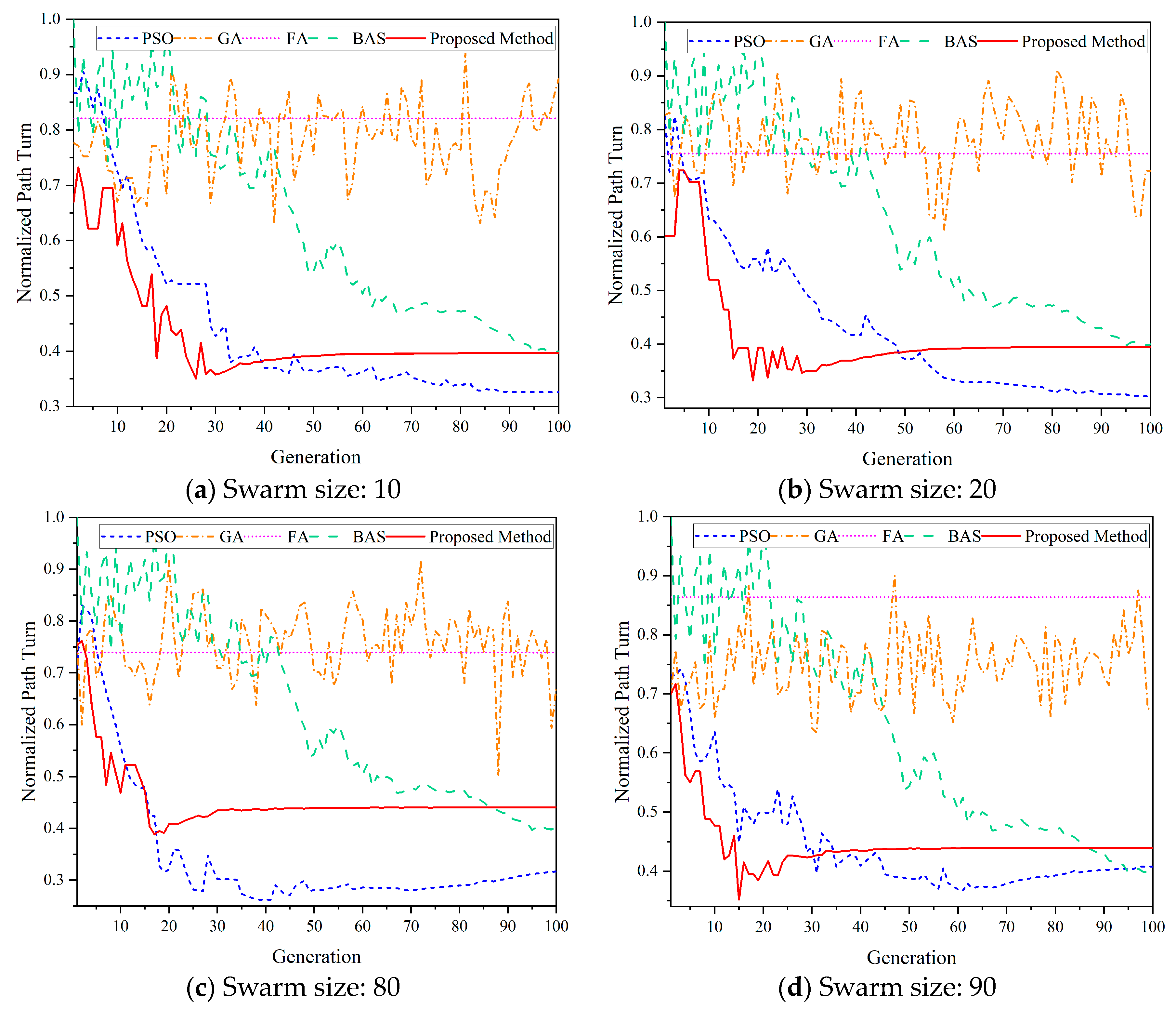
Figure 9 shows the effects of the swarm sizes on the turning angles. It is known that the path should be as straight as possible for the UAVs to follow, and smaller turning angles on a UAV path are desired. In Figure 9, for GA and FA, the two algorithms cannot locate the global best solutions in the given iterations. GA fluctuates violently until the last iteration. FA falls into a local optimum and cannot get out. Thus, the sums of the turning angles of FA become the biggest. For standard BAS with different swarm sizes, there are many fluctuations before 45 iterations. It is because only one beetle exists to find the optimum solutions, which makes the swarm social information quite limited, and it cannot be shared. PSO works well and can find the global best solution successfully. However, its convergence rate is much slower than that of the proposed BSO method in all the circumstances. Usually, more than 50 iterations are needed for PSO to find the best solutions.

There is no doubt that the proposed BSO method could converge within 30 iterations. Especially when the swarm size is 80, only about 20 iterations are needed. Interestingly, the final optimum turning angles of a path generated by the proposed BSO method are larger than that of PSO. It is even larger than that of standard BAS when the swarm size is set as 80 and 90, respectively. That is because the overall global optimum solutions are obtained by sacrificing the turning angles when the path is generated using the proposed BSO method. In some situations, the priority of the effective factors should be higher than the turning angles within the limitations of the UAVs themselves, such as the path risk, path length, and path smoothness. If the turning angles are on an accepted level, it will be alright for the UAVs to follow.

Figure 10 shows the effects of different swarm sizes on the path length. It is obvious that the path length of the proposed BSO is the shortest, no matter how many individuals there are in a swarm. Meanwhile, the rate of convergence is the fastest of all, which further proves that the global best solutions could be found within 30 iterations in all kinds of conditions compared with algorithms.

As shown in Figure 10, when the swarm size is larger than 20, PSO works better than standard BAS. If there are fewer individuals in a swarm, for example, the swarm size is 10, the path generated by standard BAS is better with a shorter flying distance after the 75^th iteration. GA and FA are worse than the other three. For FA, it will fall into the local optimum quickly when it starts, which leads to the path length staying the same with no changes. It also proves that FA could only provide one flying path when it runs, which may not be the best. Oppositely, for GA, there are a lot of drastic fluctuations in the UAV path length in the optimization process. This is because the GA algorithm is always trying to locate the optimum solutions, but it ultimately fails. The biggest difference in the path length of the five algorithms appears in Figure 10a. Based on the data provided in Figure 10, we can see that when the swarm size is set as 10, the proposed BSO method is 27.75%, 66.51%, 64.31%, and 23.20% better than PSO, GA, FA, and standard BAS, respectively.

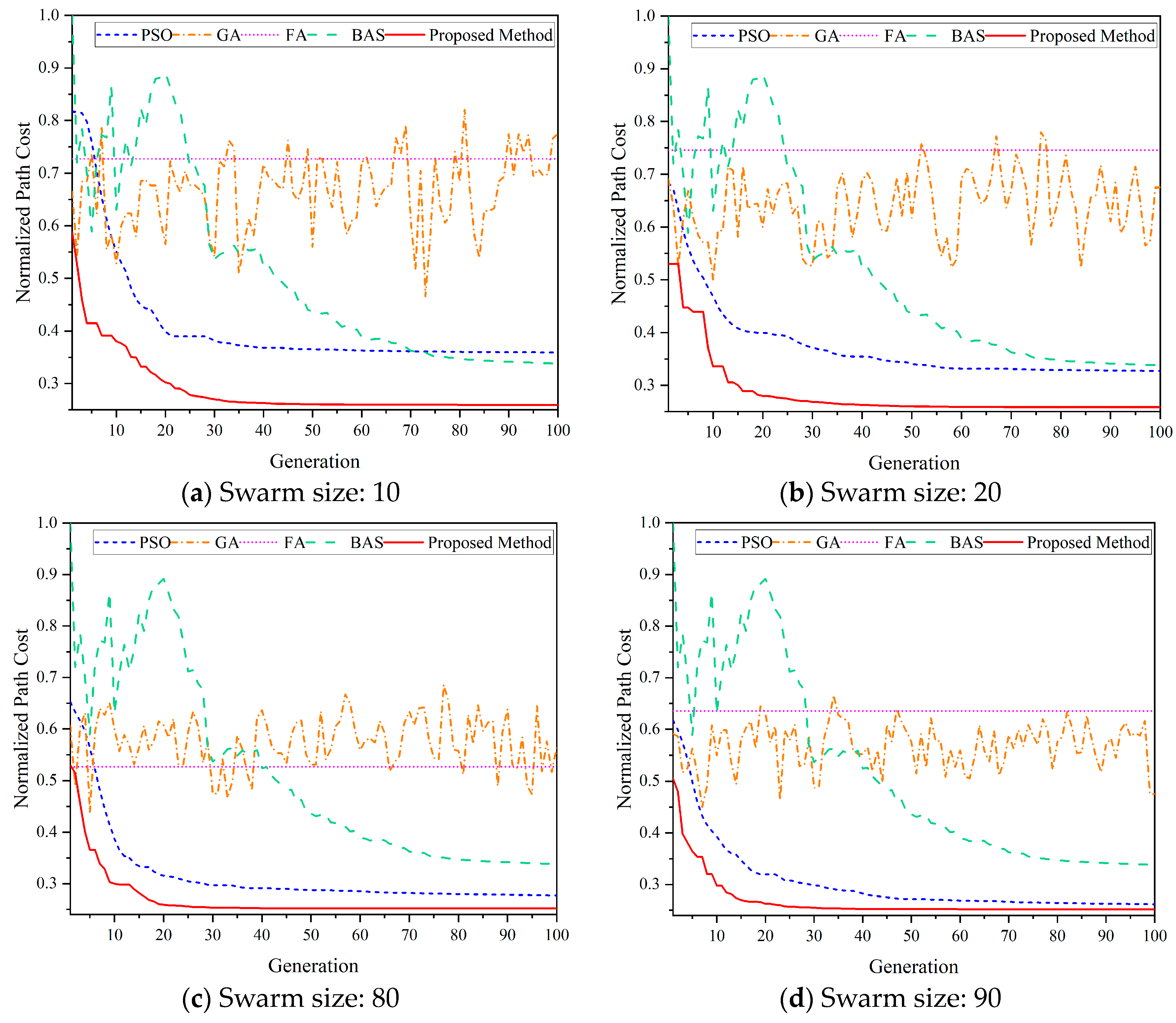
The overall cost of a generated UAV path, including the ground risk, turning angles, and path lengths, is shown in Figure 11. From the figures, we can see that the path cost of the proposed BSO method is the lowest under all kinds of swarm size settings. It converges quickly and locates the global optimum solutions within 20 iterations. After that, it becomes the smoothest of the five. Combined with Figure 9, it can be concluded that the proposed BSO algorithm obtains a UAV path with the lowest overall cost by sacrificing the larger turning angles, which is satisfied with the UAV’s performance limitations. PSO performs similarly to the proposed BSO method. However, its rate of convergence is much lower, and as a result, more iterations are needed. The path cost of PSO is higher than that of the proposed BSO method under all the conditions of different swarm sizes. The biggest difference is as much as 27.74% when the swarm size is set as 10.

From Figure 11, for standard BAS, at the beginning of a few iterations, there are a lot of fluctuations, and it becomes much smoother after 40 iterations, regardless of the swarm sizes. It is because only one beetle in standard BAS could not determine the optimum search directions because of the lack of global information. In this way, more iterations are needed. When the number of individuals in the swarm is 10, the overall path cost of standard BAS is better than that of PSO after 75 iterations, which is improved by 5.92%. It means that PSO is highly affected by the swarm size and can only work well with more individuals. Based on the given path cost, GA still cannot locate the global best waypoints. It always fluctuates from position to position. GA would have a strong randomness, which makes it hard to plan an optimal flying path for the UAVs. Similarly, FA easily falls into the local optimum at the beginning and until the end. The path it generates may not be the best, although a flying path is indeed obtained. It may be suitable for the UAVs to follow but with a much higher cost compared with PSO, standard BAS, and the proposed BSO method in this scenario.

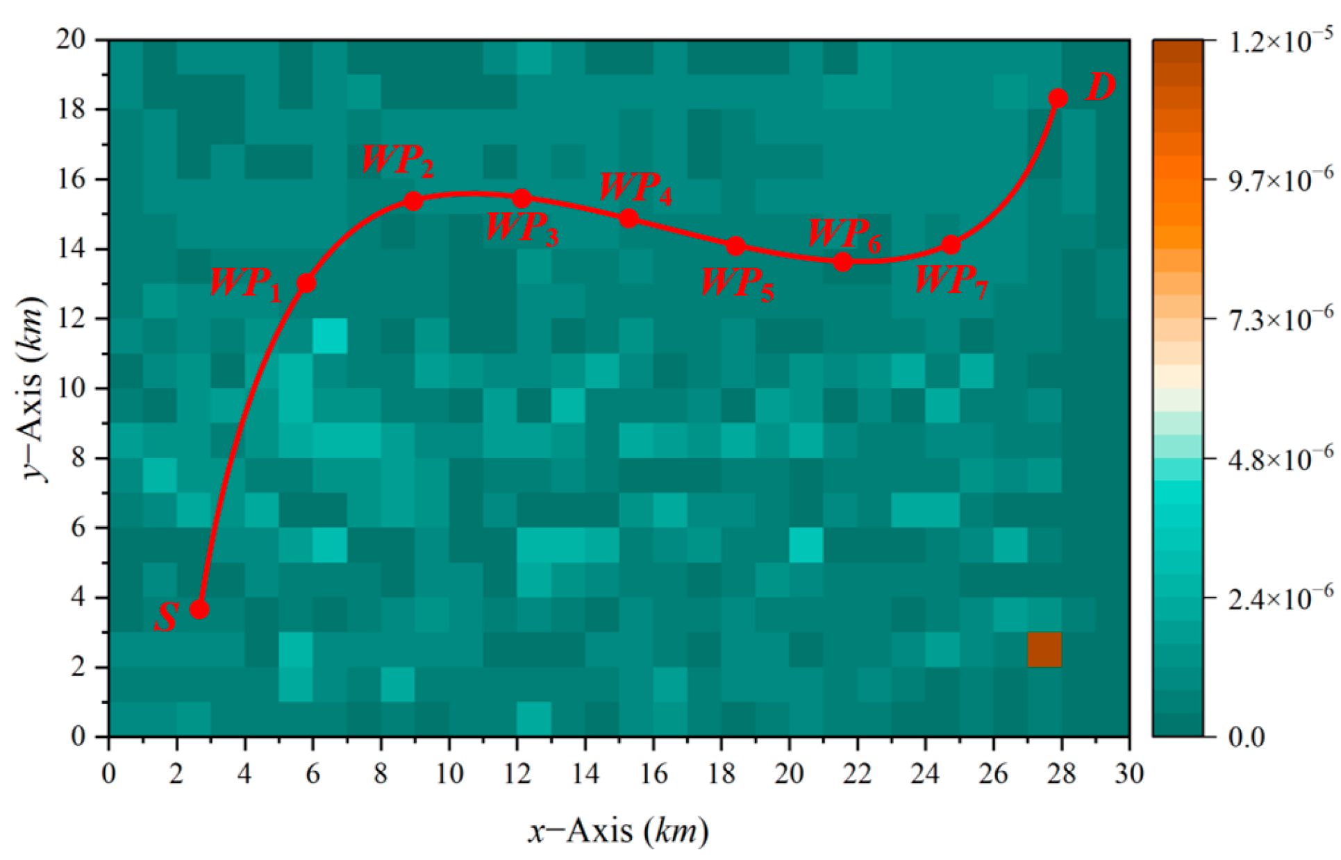
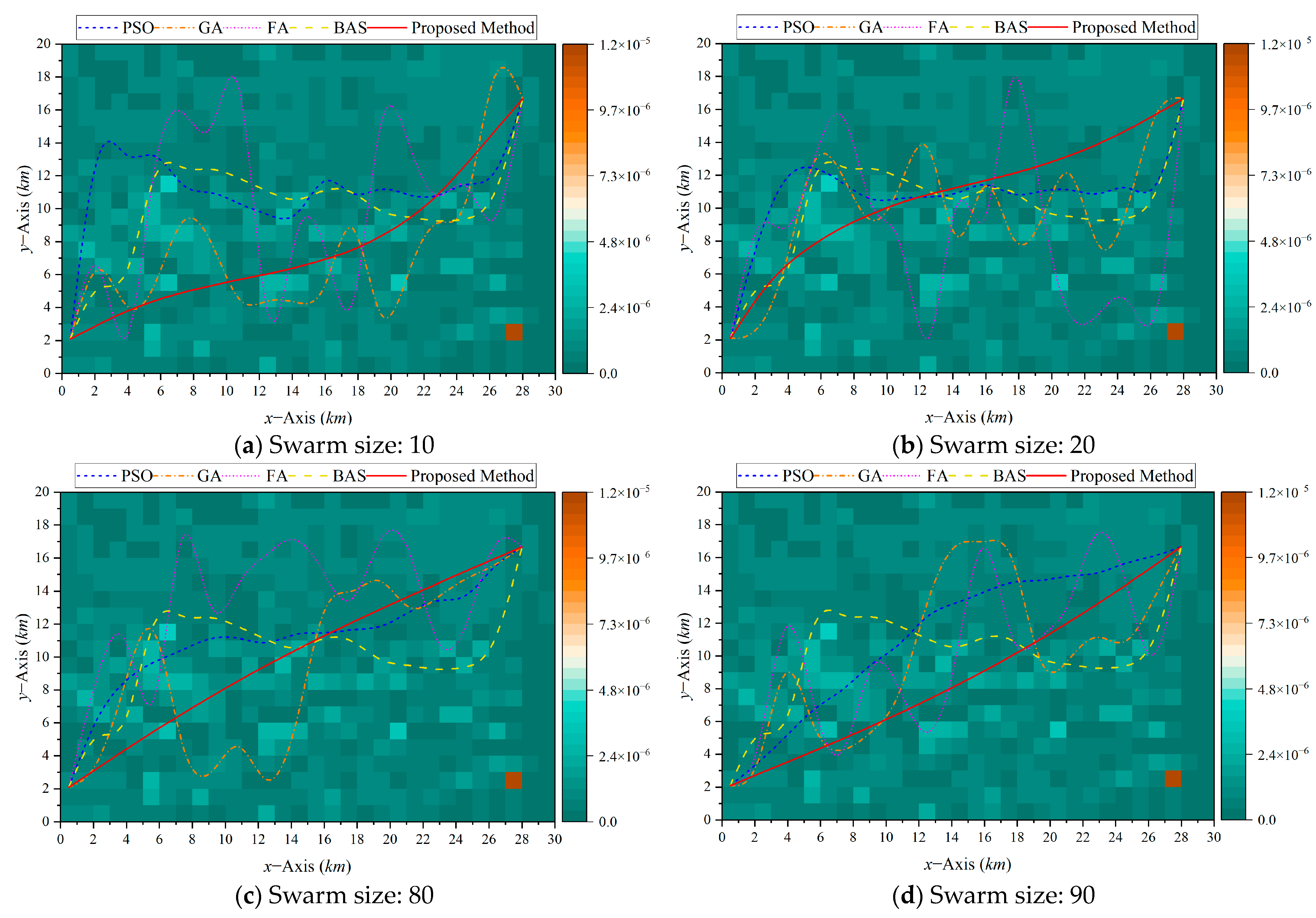
The generated UAV paths in a 2D environment by the five algorithms concerning a ground risk map are provided in Figure 12 with different swarm sizes. Theoretically, an optimum UAV path should avoid the ground areas with high risk to make the ground people as safe as possible. As shown in Figure 12, when the swarm size is 10, FA jumps all the time from the beginning to the end. If the UAVs follow the paths provided by FA, they have to turn a lot and frequently. GA is better than FA, with fewer troughs and peaks of waves. PSO and standard BAS are similar to some extent, both of which are much smoother than GA and FA. When there are 20 individuals in a swarm, GA and FA do not change a lot, but there are still many fluctuations. Standard BAS stays the same in the four parameter settings because the swarm size can not affect it at all. PSO becomes more gentle as the swarm size becomes larger and larger. However, the proposed BSO method in this work performs the best with fewer turns on the path and when it is much closer to a straight line that connects the starting point S and destination point D in the operation scenario. It is such an expected situation that it is desirable for the UAVs to follow easily and safely.

Based on the provided paths in Figure 12, when the swarm size is set as 80 and 90, respectively, the path generated by the proposed BSO method becomes an approximate straight line. It is not only easy for the UAVs to follow it, but it also has a short length to save energy consumption significantly. PSO works a little better with more individuals. The larger swarm sizes would normally make it locate more accurate solutions. Furthermore, GA and FA could also find better waypoints with the help of more individuals. It is obvious that the fluctuations of the two decrease, which means there are fewer turns on the path, which makes it suitable for the UAVs to follow.

5.3. Effects of Individual Dimensions

In this subsection, the effects of the different individual dimensions in a swarm are explored and presented, which are set as 15, 20, 25, and 30. The swarm size and the number of iterations are set as 20 and 100, respectively.

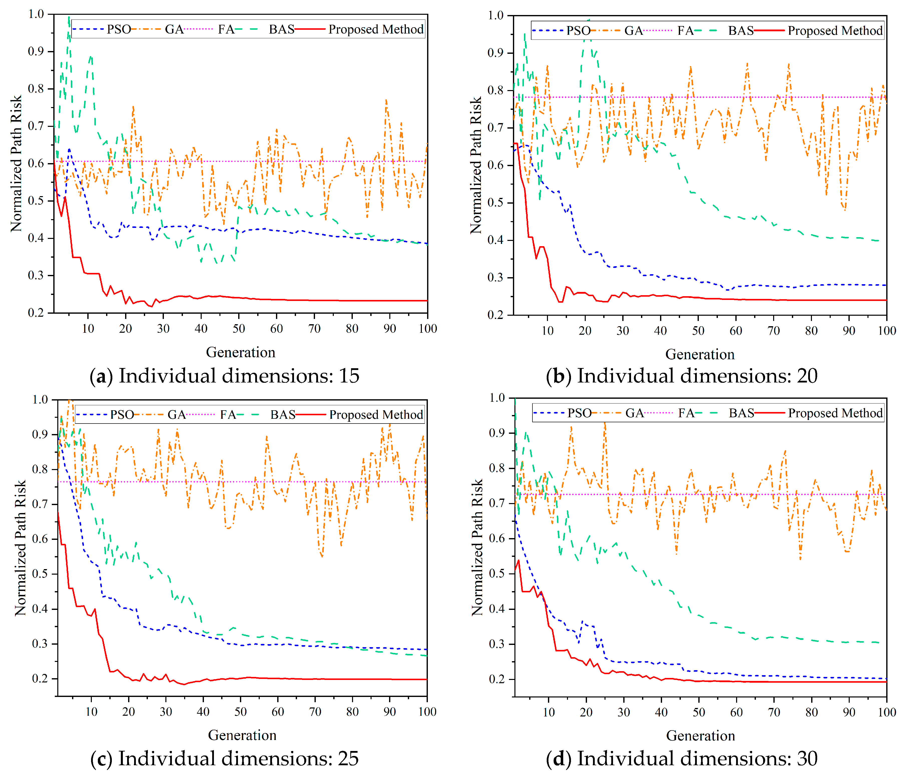
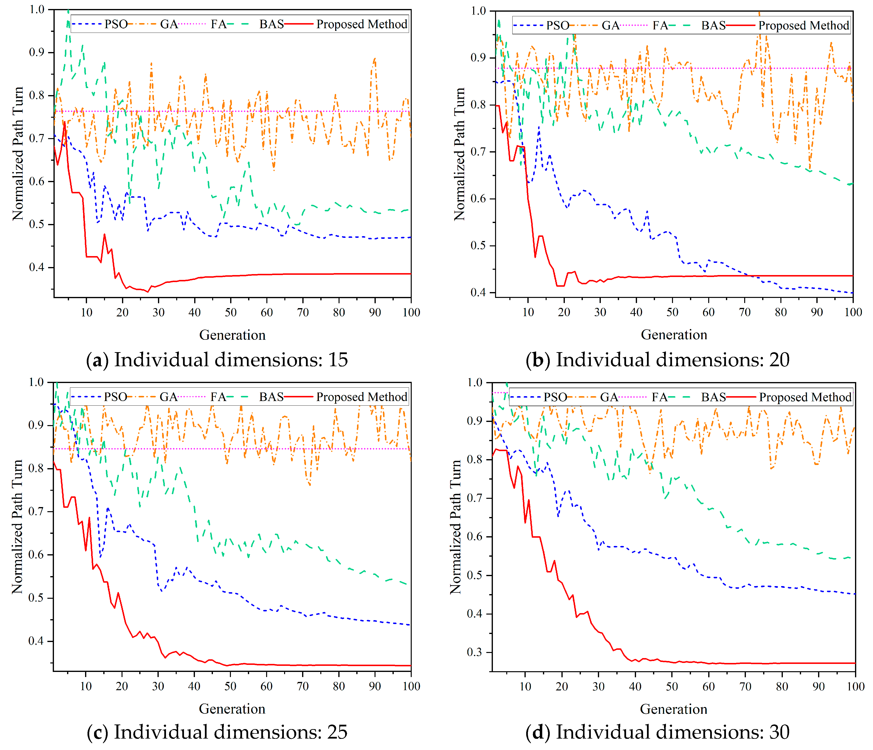
Figure 13 illustrates how the path risk can be affected by the individual dimensions. There is no doubt that the proposed BSO method could generate a path with the lowest risk, no matter what the individual dimensions are. Also, the rate and efficiency of convergence are the best of the five. The global optimum waypoints are found within 50 iterations. PSO can provide a sub-optimum solution compared with the proposed BSO method, which produces a higher path risk on the ground. The convergence rate and efficiency of PSO are both worse than those of the proposed BSO method. There are more fluctuations on the ground risk curves given by standard BAS, especially in the first few iterations. But it will be improved as the higher individual dimensions are set. The ground risk of a UAV path produced by standard BAS is higher than that produced by PSO. But when the individual dimension is 15, the path risk of standard BAS is a little lower than that of PSO in the 100th iteration. GA and FA are the worst of all under all the conditions. It is difficult for GA to locate the optimum solutions. FA falls into the local optimum and cannot get out in the whole optimization process.

Based on the data in Figure 13, the path risk of the proposed BSO method is 39.72%, 64.90%, 61.58%, and 39.04% lower than that of PSO, GA, FA, and standard BAS with the individual dimensions of 15, which proves the proposed BSO method is quite suitable for the limited individual dimensions.

Figure 14 shows the sum of the turning angles on the generated UAV paths with the different individual dimension settings.

It is obvious that when the dimensions are set as 15, 25, and 30, the turning angles of the proposed BSO method are the best. However, PSO is a little better than BSO under the condition of the individual dimension of 20 after the 72^nd iteration. Combined with the results provided in Figure 9, the turning angles are used to offset the path risk to guarantee the safety of the people on the ground, which is satisfied with the optimization objectives. PSO is worse than the proposed BSO method but better than the other three, with much fewer turning angles. The individual dimension generates a great number of effects on standard BAS. The high dimensions would make it more efficient and converge quickly. From the figure, we can see that both GA and FA fail to find the global best waypoints. GA fluctuates acutely from the beginning to the end, with a lot of turnings on the generated path. FA falls into the local optimum in the first iteration. The biggest improvements of the proposed BSO method are 39.72%, 69.40%, 72.04%, and 50.20% better compared with PSO, GA, FA, and standard BAS with an individual dimension of 30.

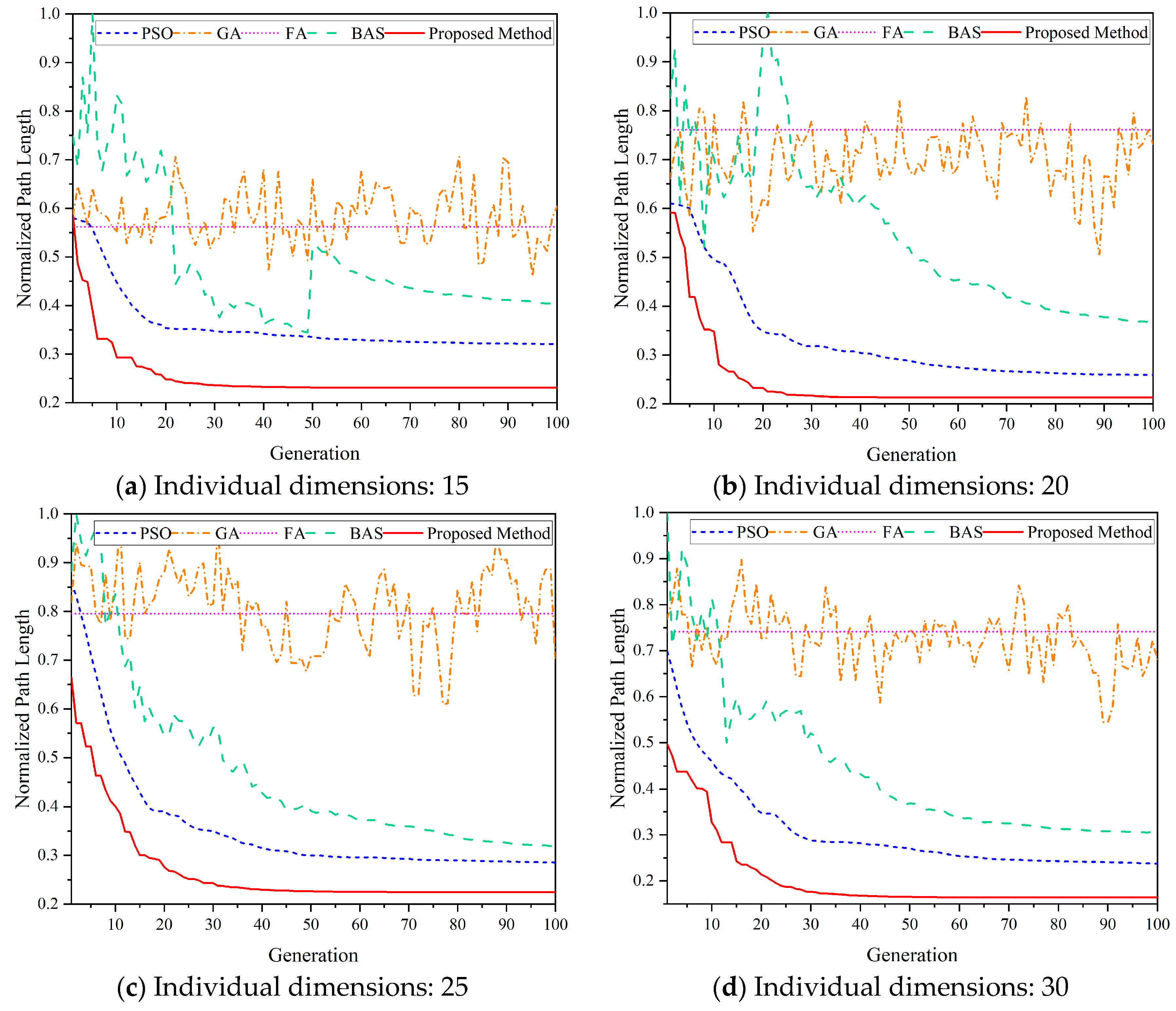
The path lengths of the five different algorithms are provided in Figure 15. GA and FA are the worst of all. GA fluctuates frequently to try to find the best solutions all the time. But it cannot even get closer to the best positions in the search space. In this way, the global best cannot be found but with a lot of fluctuations in the search process. FA falls into the local optimum at the beginning and would not change at all. The path lengths of the two are the longest In the last Iteration. Standard BAS, PSO, and the proposed BSO method present the same downward trends. However, standard BAS will jump a lot in the first few iterations because only one beetle exists to locate the optimum solutions, which makes it inefficient and impossible. PSO can calculate the positions of the best waypoints with higher efficiency and quicker convergence. But it is worse than the proposed BSO method. By using the proposed BSO, the global best can be found only within 30 iterations, as well as the shortest path lengths. Even with the lowest individual dimension of 15, the proposed BSO method is still 28.10%, 61.79%, 58.95%, and 42.72% better than PSO, GA, FA, and BAS in the UAV path length, respectively.

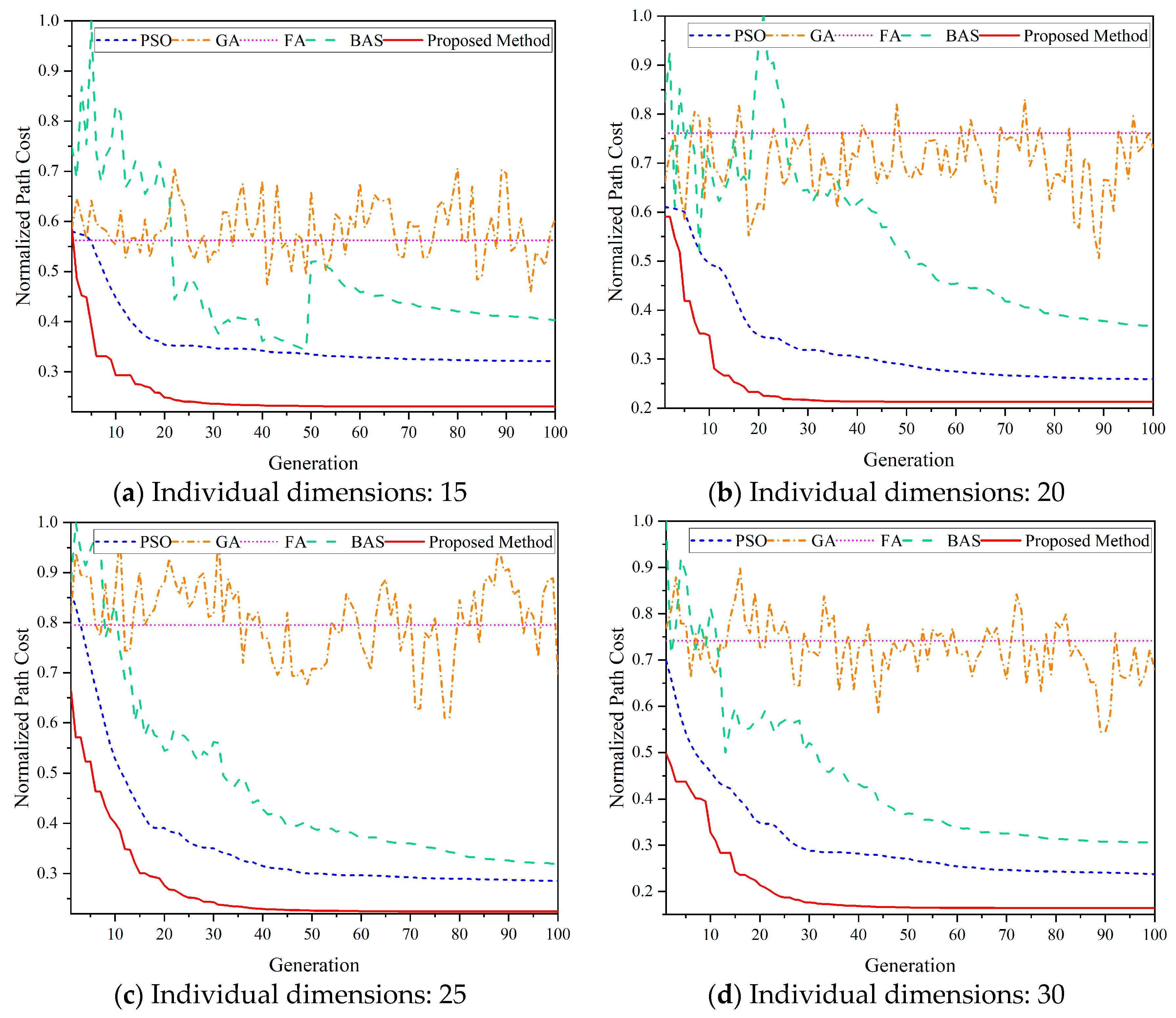
The overall cost of the generated paths by the five algorithms is provided in Figure 16. From all the curves, we can see that our proposed BSO method works well under all the individual dimension settings with the minimum path cost. Also, the optimal waypoints can be found as soon as possible once it starts running. Particularly when the individual dimension is set as 20, only 30 iterations are needed to locate the global best solutions. It is smooth enough that there are no big fluctuations in the cost curves in all the circumstances.

From Figure 16, we can see that PSO works as stably as the proposed BSO method. However, the path cost it generates is more than that of the proposed method, which is much better than the other three with the lower cost and the quicker convergence. Standard BAS would go through a lot of ups and downs in the first few iterations to find the correct optimization fields. However, when the dimensions of the beetle get higher, such as 25 and 30, the ups and downs would be fewer and fewer. Even though the final cost is a little more than that of PSO, 11.52% and 28.51%, respectively, with the dimensions of 25 and 30. GA and FA are the worst of all. For FA, it falls into the local optimum so easily that the cost of the UAV path will not change after the iteration starts. However, there is so much randomness during the optimization of GA. In this way, ups and downs would exist in the whole optimization process. GA cannot find optimum solutions, which is not suitable to solve continuity problems like this. When the individual dimension is set as 30, the proposed BSO method is 31.00%, 75.86%, 77.87%, and 46.31% better than PSO, GA, FA, and standard BAS in the normalized path cost.

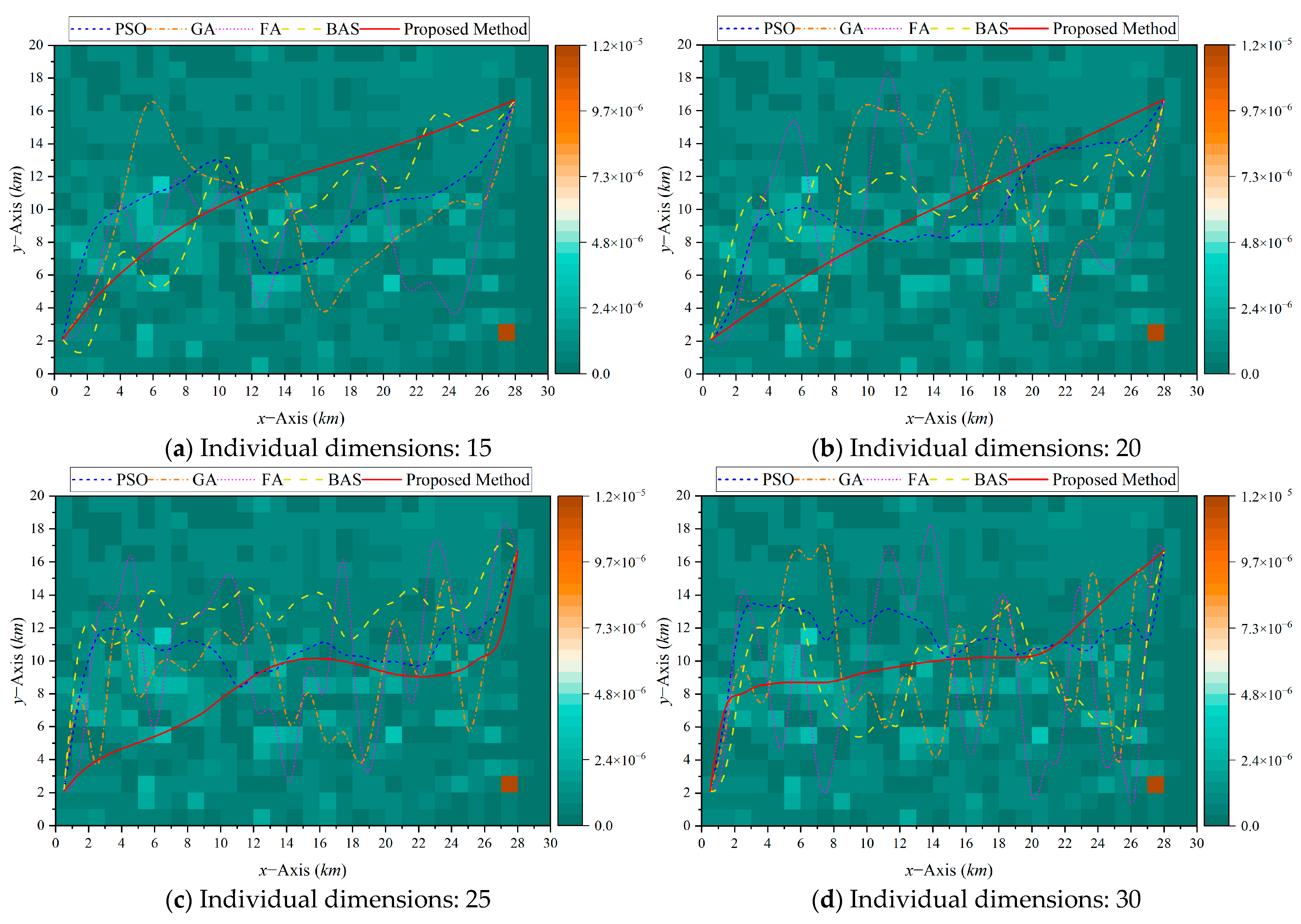
The generated UAV paths are provided in Figure 17. From this figure, it can be seen that all the listed five algorithms could generate the paths for the UAVs, but with quite different smoothness and fluctuations. It is desirable to keep the paths as smooth as possible so that the UAVs can easily follow them. In this way, it is obvious that the path provided by the proposed BSO method is the smoothest under all the conditions with the fewest turns on the paths. Especially when the individual dimension is 20, the given path is nearly a straight line that connects the starting point S and destination point D directly.

As Figure 17 shows, we can see that the higher individual dimensions would generate very negative effects, which correspondingly bring more turns. PSO could find an optimal flying path for the UAVs under all the settings. But there are more turns on the path compared with the proposed BSO method. Especially when the dimension is 30, the path of PSO is the most fluctuant compared with others. All the UAVs have to turn all the time to achieve a lower path cost. Standard BAS is in the middle position, which is better than GA and FA but worse than the proposed BSO method and PSO. The corresponding amplitudes of the variations are much better than GA and FA. Obviously, FA is the worst, which jumps all the time from the beginning to the end, trying to make the path cost the global optimum. Combined with the previous results, this is caused by the local optimum problem. No more better waypoints can be provided. GA presents similar characteristics to FA, but the amplitude of the fluctuation is a little smaller because GA is always trying to locate an optimum solution, even though it fails in the end. Oppositely, the quality of GA’s solution is higher than that of FA’s. In this way, the path given by GA is much smoother than FA.

5.4. Effects of Iterations

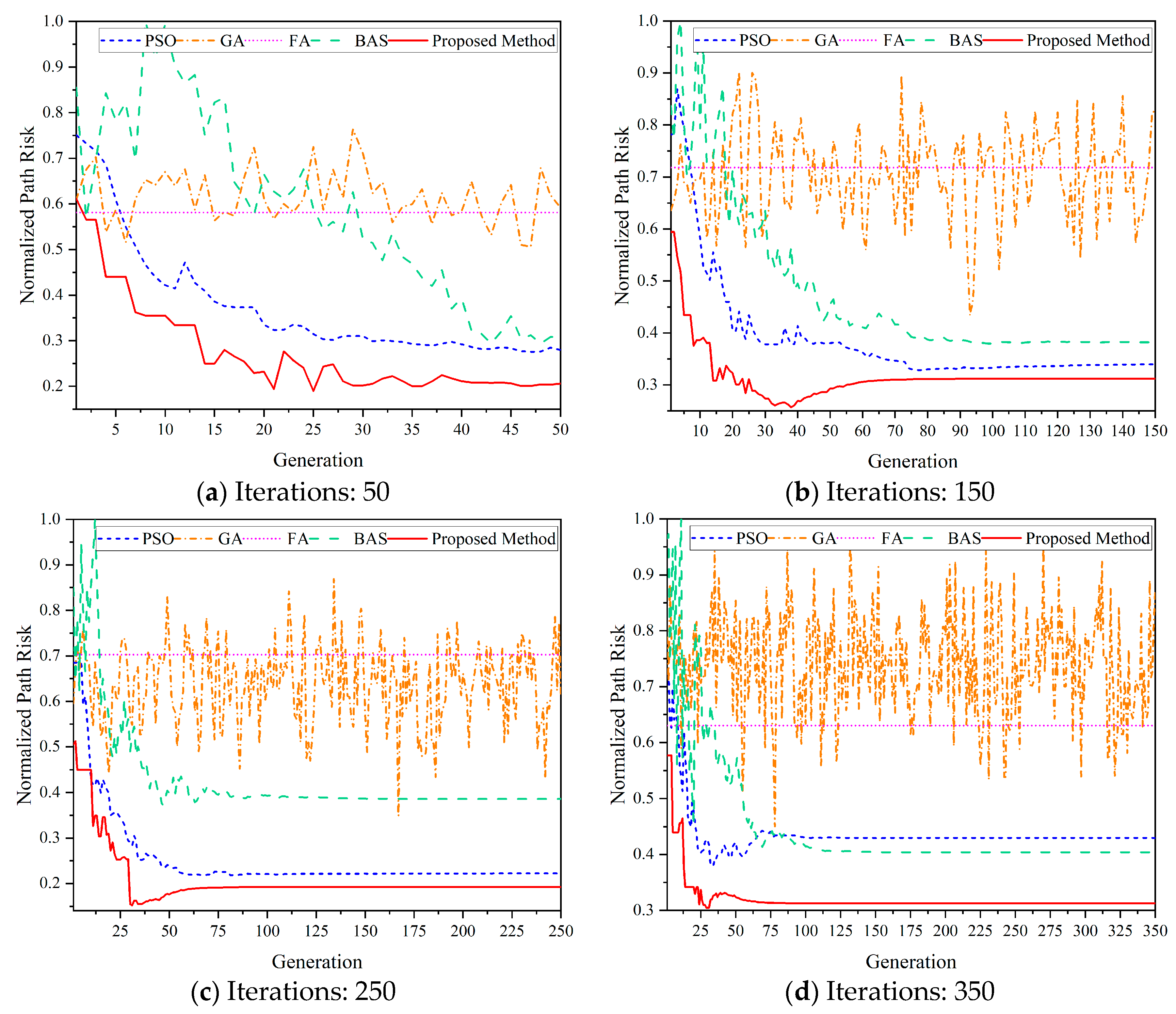
In order to explore the convergence rate of the proposed BSO method, the effects of the different numbers of iterations are analyzed in this subsection. In these simulations, the numbers of the algorithm iterations are set as 50, 150, 250, and 350, respectively. Still, the path risk, turning angle, path length, total path cost, and generated UAV paths are the indexes that are used to evaluate the performances of the algorithms.

Figure 18 presents the normalized risk of the generated UAV paths under the different iteration settings. From the curves, we can see that the proposed BSO method becomes quite stable within only a few iterations. As shown in Figure 18a, 50 iterations are enough to locate a solution for the UAV’s waypoint set. Combining with the curves in Figure 18b, the global best solutions would be found around the 70th iteration. After that, the risk of the UAV path does not change a lot. It becomes much more obvious, as shown in Figure 18c,d, with 250 and 350 iterations, respectively. In this way, for the proposed BSO method, not so many iterations are needed to find the global best solutions, which further guarantees time efficiency. Meanwhile, there are not so many fluctuations except for the very few beginning iterations.

The trend of PSO is similar to that of the proposed BSO method, as presented in Figure 18. But the path risk imposed by PSO is much higher in every generation. The path risk of standard BAS is higher than PSO and BSO. Meanwhile, there are more ups and downs, especially in the first 50 iterations, as shown in Figure 18a. More than 100 iterations are needed for standard BAS to obtain a relative optimum solution based on Figure 18b–d. When there are 350 iterations, the risk of standard BAS is lower than that of PSO after the 80th iteration. GA and FA are the worst of all. More iterations give GA more fluctuations since the beginning. As described in Figure 18d for GA, each jump in each generation is so different, which illustrates GA cannot locate the optimum solutions accurately. Quite differently, the path risk of FA under all the iteration settings stays the same from the beginning to the end. It means that FA falls into the local optimum quickly, no matter how many iterations there are. It is 27.23%, 64.14%, 50.36%, and 22.56% lower in the path risk of the proposed BSO method than PSO, GA, FA, and standard BAS.

Figure 19 shows the accumulated turning angles on a given UAV path by the five algorithms with the different iterations. From the curves, it can be seen that in the few beginning iterations, there would be fluctuations for the proposed BSO method, PSO, and standard BAS. However, the convergence rates of the proposed BSO method are the best of the three.

Based on Figure 19b–d, there are more turning angles on the UAV path generated by the proposed BSO method than PSO after the 32nd, 98th, and 41st iterations. After that, the turning angles of the two would remain stable until the end. Considering the previous analysis, the proposed BSO method guarantees the lowest path risk as well as the shortest UAV path by sacrificing the turning angles, which makes sense in the actual operations. Standard BAS is worse than the two above on the turning angles, with more ups and downs. According to the curves provided in Figure 19, for standard BAS, more than 110 iterations are needed to reach the optimum positions because, in BAS, only one beetle is used to locate the best in each move. GA and FA are the worst of all. The turning angles of FA are determined at the beginning and would not change anymore, which is because the local optimum solutions are found and are taken as the global optimum waypoints. This drawback of FA cannot be overcome by itself. Oppositely, GA changes all the time in every iteration. As shown in Figure 19, GA cannot find consistent solutions, which makes it jump from iteration to iteration. It seems that it jumps around a possible solution but will never reach it. Actually, GA is suitable to solve the discrete problems instead of the continuous ones, such as path planning considering the ground risk. Especially for this kind of multi-objective optimization problem in a given solution space, the performances of GA will be quite poor and cannot satisfy all the constraint conditions.

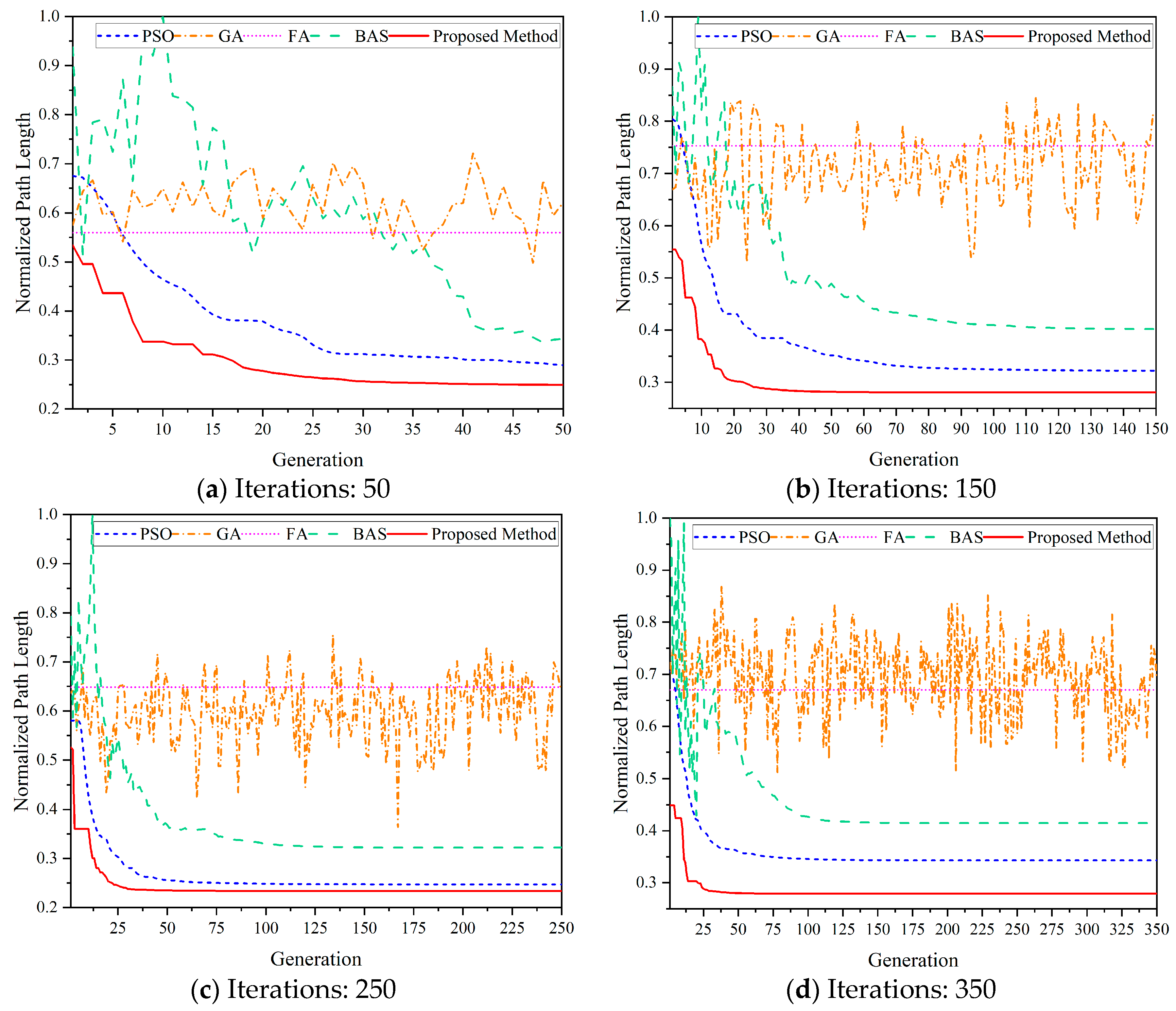
The path lengths of these different algorithms with the effects of the iterations are presented in Figure 20. It is obvious that the proposed BSO method is the best, with the shortest path length under all kinds of iteration settings. Also, its rate of convergence is the fastest, and it can complete around 30 iterations. PSO is similar, but the rate of convergence is lower than the proposed one. Generally, 70 iterations are needed for PSO based on the data provided in Figure 20. The final normalized path length of PSO is longer than that of the proposed BSO method under all the conditions. Standard BAS is worse than the aforementioned two but better than GA and FA. A lot of ups and downs exist in the beginning, and after that, it becomes stable until the convergence, but with a much longer path in the final iteration. FA and GA are the worst, with the longest paths. For FA, once it starts, the path length would remain the same without any changes. It proves that FA cannot locate the optimum solutions, and the first generated one will be seen as the global best, which is then kept in the whole optimization process. As a matter of fact, it is far away from the true optimum values. GA will fluctuate all the time, trying to obtain the global optimum solutions. However, because of the existence of the strong randomness, it cannot reach but only moves around it. As presented in Figure 20, the normalized path lengths undulate from iteration to iteration for GA. The final obtained waypoints may also not be the global best. Compared with PSO, GA, FA, and standard BAS, the proposed BSO is 18.59%, 59.66%, 58.30%, and 32.64% shorter in the normalized path length, respectively.

The overall path cost of the five algorithms can be found in Figure 21. There is no doubt that more iterations would make both of the proposed BSO and PSO algorithms become more smooth. That is because by evolving more generations, the individuals in a swarm would move closer and closer to the true optimum solutions in the search space. However, the total cost of the path generated by PSO would be higher than that of the proposed BSO method under all the conditions in Figure 21. Also, more iterations can smooth the curves of standard BAS because, by going through more iterations, the beetle would move more steps towards the best position. Correspondingly, the path cost would become more stable. But the values are higher than the proposed BSO method as well as PSO.

As shown in Figure 21, GA and FA are the worst of the five. Ultimately, the total path costs of the two are the highest out of all options. GA jumps all the time from the first iteration to the last one, no matter how many iterations there are. It always fails to locate an optimum solution in this scenario. From the curves, we can see that GA would fluctuate a lot around a certain value but will never reach it. That is because GA belongs to a kind of discrete algorithm in that the cost values would be separated during two consecutive iterations. It will be more obvious when there are more iterations, as shown in Figure 21c,d. From the normalized path cost given in the figure, it is a straight line for FA, which is because a fake optimum value is found and is then used as the global best. The local best is the problem that cannot be overcome by FA when it is trying to locate an optimum solution in the search space. Even though there are 350 iterations for FA, as shown in Figure 21d, the path cost of FA still remains the same in the end, which is determined by itself. Based on the data provided in Figure 21, the proposed BSO method is 18.57%, 59.66%, 58.30%, and 32.63% better than PSO, GA, FA, and standard BAS.

The effects of the iterations on the generated UAV paths are provided in Figure 22. From the curves, the path generated by the proposed BSO method is the smoothest, besides the fewest turns on it. It proves that it is quite suitable for the UAVs to follow. Also, combined with the previous results, the cost of the UAV path given by the proposed BSO method is the lowest. All in all, the number of iterations could generate quite limited effects on the proposed BSO method, which, as a result, proves its accuracy and robustness. It would converge as soon as possible without too many iterations. But, oppositely, the number of iterations affects the other four algorithms a lot. For example, for PSO, more iterations would make the path smoother. Especially in Figure 22c, when the iteration is 250, PSO could generate a similar path to the proposed BSO method but with more turns on the path. If the particles in PSO evolve more generations, the solutions are much closer to the true global best. But more generations introduce more time consumption correspondingly. Standard BAS is highly dependent on the iterations, too, because if the beetle makes more moves, it becomes closer to the optimum position. There are a great many turns on the paths produced by GA and FA, regardless of the number of iterations. Of course, the iterations have positive effects on GA and FA. More iterations make the two algorithms obtain relatively optimum solutions, which makes the generated paths easy for the UAVs to follow. But as a whole, neither GA nor FA would give the perfect flying paths as the proposed BSO method.

5.5. Comparisons with Dijkstra and A* Algorithms

In this subsection, the proposed BSO method is compared with Dijkstra and A* algorithms to better evaluate its performance. In the simulation, the two parameters, including the swarm size and individual dimension of the proposed BSO method, are set as 20 and 15, respectively. Its number of iterations is 150.

Table 2. Cost comparisons with Dijkstra and A* algorithms.

Item	Dijkstra Algorithm	A* Algorithm	Proposed Method
Path risk	1.00	0.79	0.36
Turning angles	1.00	0.83	0.37
Path length	1.00	0.79	0.36
Path cost	1.00	0.86	0.48

below gives the cost comparisons of these three path-planning algorithms. In this table, the normalized path risk, turning angles, path length, and path cost are provided.

From the table, it can be found that the path risk of the proposed BSO method is the least of all, which proves that the generated path is the safest when it is followed by the UAVs. It is 64.00% and 54.43% safer than Dijkstra and A* algorithms. The turning angles and path length of the proposed BSO method are still the best of the three, which are 63.00% and 55.42% better in turning angles and 64.00% and 54.43% better in path length compared with Dijkstra and A* algorithms, respectively. The overall path cost of the proposed BSO method is the lowest compared with Dijkstra and A* algorithms, which are improved by 52.00% and 44.19%, respectively. Furthermore, the A* algorithm is better than the Dijkstra algorithm in all the performance indexes provided in Table 2. Dijkstra algorithm works the worst in this path-planning scenario, especially considering the ground risk, which means that the global optimum path is not found at all.

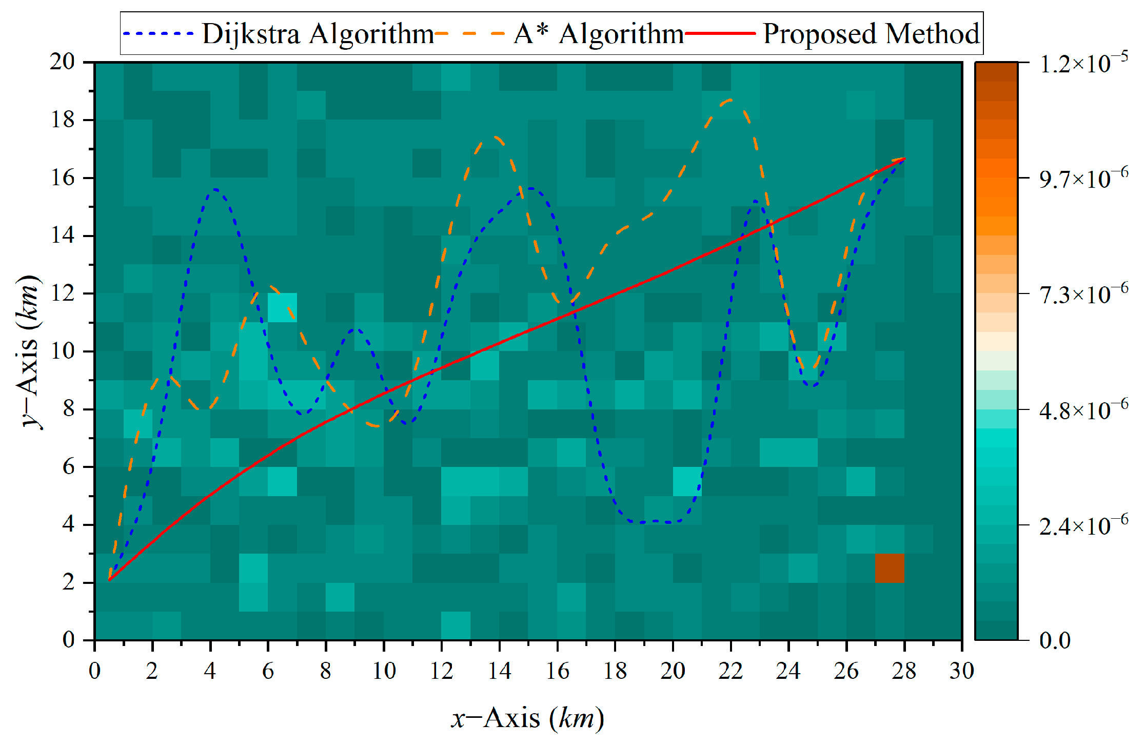
The UAV path considering the ground risk distributions generated by the aforementioned three algorithms is shown in Figure 23. From this figure, all three paths generated by these algorithms are always trying to be away from the southeastern areas, whose ground risk is higher. It can be found that the path produced by the proposed BSO method is the closest to the straight line connecting the starting point and the destination point with the least path cost based on the data provided in Table 2. Additionally, the A* algorithm is better than the Dijkstra algorithm, with fewer turning angles and a shorter path length. The Dijkstra algorithm is the worst of all, and it is not suitable for the UAVs to follow with the highest ground risk as well as the longest path length and the most turning angles. All in all, the path provided by the proposed BSO method is the smoothest with the lowest flying cost and has proved to be the most suitable for UAVs to follow.

6. Conclusions

In this paper, a beetle swarm optimization (BSO)-based path-planning algorithm for UAVs in urban environments is proposed by considering the ground risk distributions. The ground risk map is incorporated into the planning model to guarantee the safety of the people on the ground, as well as the smallest turning angles and the shortest flying path. According to the ground risk map, a path box is generated in the BSO method to quantize the path risk. Subsequently, an adaptive step size for every beetle and a random proportionality coefficient are designed to improve the accuracy and the convergence problems that usually appear in standard beetle antennae searches (BAS). After that, a global optimum attraction operator is proposed to share the social information in a swarm to lead all the beetles to move to a better position. Finally, a case study and comparisons are made with PSO, GA, FA, and standard BAS under three different scenarios. The results show that the proposed BSO method outperforms the other four heuristic algorithms not only in efficiency but also in accuracy with high robustness and flexibility, which strongly confirms the suitability of the proposed approach.

References

1. Phung, M.D.; Ha, Q.P. Safety-enhanced UAV Path Planning with Spherical Vector-based Particle Swarm Optimization. Appl. Soft Comput. 2021, 107, 107376. [Google Scholar] [CrossRef]
2. Abbas, N.; Abbas, Z.; Liu, X.; Khan, S.S.; Foster, E.D.; Larkin, S. A Survey: Future Smart Cities Based on Advance Control of Unmanned Aerial Vehicles (UAVs). Appl. Sci. 2023, 13, 9881. [Google Scholar] [CrossRef]
3. Gao, X.; Xiao, G.; Xie, K.; Wang, W.; Fu, Y.; Chang, C.; Wang, Z. A Framework of Modeling and Simulation Based on Swarm Ontology for Autonomous Unmanned Systems. Appl. Sci. 2023, 13, 9297. [Google Scholar] [CrossRef]
4. Hu, X.T.; Pang, B.Z.; Dai, F.Q.; Low, K.H. Risk Assessment Model for UAV Cost-effective path planning in Urban Environments. IEEE Access 2020, 8, 150162–150173. [Google Scholar] [CrossRef]
5. Primatesta, S.; Rizzo, A.; La Cour-Harbo, A. Ground Risk Map for Unmanned Aircraft in Urban Environments. J. Intell. Robot. Syst. 2020, 97, 489–509. [Google Scholar] [CrossRef]
6. Chen, J.C.; Du, C.L.; Zhang, Y.; Han, P.C.; Wei, W. A Clustering-based Coverage Path Planning Method for Autonomous Heterogeneous UAVs. IEEE Trans. Intell. Transp. Syst. 2021, 23, 25546–25556. [Google Scholar] [CrossRef]
7. Kavraki, L.E.; Svestka, P.; Latombe, J.C.; Overmars, M. Probabilistic Roadmaps for Path Planning in High-Dimensional Configuration Spaces. IEEE Trans. Robot. Autom. 1996, 12, 566–580. [Google Scholar] [CrossRef]
8. Xu, Z.F.; Deng, D.; Shimada, K. Autonomous UAV Exploration of Dynamic Environments Via Incremental Sampling and Probabilistic Roadmap. IEEE Robot. Autom. Lett. 2021, 6, 2729–2736. [Google Scholar] [CrossRef]
9. Zhao, C.; Zhu, Y.F.; Du, Y.C.; Liao, F.X.; Chan, C.Y. A Novel Direct Trajectory Planning Approach Based on Generative Adversarial Networks and Rapidly-Exploring Random Tree. IEEE Trans. Intell. Transp. Syst. 2022, 23, 17910–17921. [Google Scholar] [CrossRef]
10. Yang, Y.; Leeghim, H.; Kim, D. Dubins Path-Oriented Rapidly Exploring Random Tree* for Three-Dimensional Path Planning of Unmanned Aerial Vehicles. Electronics 2022, 11, 2338. [Google Scholar] [CrossRef]
11. Karaman, S.; Frazzoli, E. Incremental Sampling-based Algorithms for Optimal Motion Planning. Robot. Sci. Syst. 2010, 104, 267–274. [Google Scholar]
12. Rhodes, C.; Liu, C.J.; Chen, W.H. Autonomous Source Term Estimation in Unknown Environments: From A Dual Control Concept to UAV Deployment. IEEE Robot. Autom. Lett. 2022, 7, 2274–2281. [Google Scholar] [CrossRef]
13. Pehlivanoglu, Y.V.; Pehlivanoglu, P. An Enhanced Genetic Algorithm for Path Planning of Autonomous UAV in Target Coverage Problems. Appl. Soft Comput. 2021, 112, 107796. [Google Scholar] [CrossRef]
14. Cappart, Q.; Chételat, D.; Khalil, E.B.; Lodi, A.; Morris, C.; Veličković, P. Combinatorial Optimization and Reasoning with Graph Neural Networks. J. Mach. Learn. Res. 2023, 24, 1–61. [Google Scholar]
15. Zhang, Z.; Wu, J.; Dai, J.; He, C. Optimal Path Planning with Modified A-Star Algorithm for Stealth Unmanned Aerial Vehicles in 3D Network Radar Environment. Proc. Inst. Mech. Eng. G J. Aerosp. Eng. 2022, 236, 72–81. [Google Scholar] [CrossRef]
16. Fu, Y.G.; Ding, M.Y.; Zhou, C.P.; Hu, H.P. Route Planning for Unmanned Aerial Vehicle (UAV) on The Sea using Hybrid Differential Evolution and Quantum-behaved Particle Swarm Optimization. IEEE Trans. Syst. Man Cybern. Syst. 2013, 43, 1451–1465. [Google Scholar] [CrossRef]
17. Liu, C.; Du, W.B.; Wang, W.X. Particle Swarm Optimization with Scale-Free Interactions. PLoS ONE 2014, 9, e97822. [Google Scholar] [CrossRef]
18. Roberge, V.; Tarbouchi, M.; Labonte, G. Comparison of Parallel Genetic Algorithm and Particle Swarm Optimization for Real-Time UAV Path Planning. IEEE Trans. Industr. Inform. 2012, 9, 132–141. [Google Scholar] [CrossRef]
19. Jamshidi, V.; Nekoukar, V.; Refan, M.H. Implementation of UAV Smooth Path Planning by Improved Parallel Genetic Algorithm on Controller Area Network. J. Aerosp. Eng. 2022, 35, 04021136. [Google Scholar] [CrossRef]
20. Yang, X.S. Firefly Algorithm, Stochastic Test Functions and Design Optimisation. Int. J. Bio-Inspir. Comput. 2010, 2, 78–84. [Google Scholar] [CrossRef]
21. Saadi, A.A.; Soukane, A.; Meraihi, Y.; Gabis, A.B.; Amar, R.C. UAV Path Planning using Optimization Approaches: A Survey. Arch. Comput. Methods Eng. 2022, 29, 4233–4284. [Google Scholar] [CrossRef]
22. Khan, A.T.; Cao, X.W.; Li, S. Dual Beetle Antennae Search system for Optimal Planning and Robust Control of 5-link Biped Robots. J. Comput. Sci. 2022, 60, 101556. [Google Scholar] [CrossRef]
23. Liang, Q.; Zhou, H.K.; Yin, Y.F.; Xiong, W. An Improved Beetle Antennae Search Path Planning Algorithm for Vehicles. PLoS ONE 2022, 17, e0274646. [Google Scholar] [CrossRef] [PubMed]
24. Shahid, N.; Abrar, M.; Ajmal, U.; Masroor, R.; Amjad, S.; Jeelani, M. Path Planning in Unmanned Aerial Vehicles: An Optimistic Overview. Int. J. Commun. Syst. 2022, 35, e5090. [Google Scholar] [CrossRef]
25. Liu, Y.; Zhang, X.J.; Zhang, Y.; Guan, X.M. Collision Free 4D Path Planning for Multiple UAVs Based on Spatial Refined Voting Mechanism and PSO Approach. Chin. J. Aeronaut. 2019, 32, 1504–1519. [Google Scholar] [CrossRef]
26. Primatesta, S.; Guglieri, G.; Rizzo, A. A Risk-aware Path Planning Strategy for UAVs in Urban Environments. J. Intell. Robot. Syst. 2019, 95, 629–643. [Google Scholar] [CrossRef]
27. Wu, P.P.Y.; Campbell, D.; Merz, T. Multi-objective Four-dimensional Vehicle Motion Planning in Large Dynamic Environments. IEEE Trans. Syst. Man Cybern. B Cybern. 2010, 41, 621–634. [Google Scholar] [CrossRef] [PubMed]
28. Aggarwal, S.; Kumar, N. Path Planning Techniques for Unmanned Aerial Vehicles: A Review, Solutions, and Challenges. Comput. Commun. 2020, 149, 270–299. [Google Scholar] [CrossRef]
29. Dursun, M.; Cuhadar, I. Risk based Multi Criteria Decision Making for Secure Image Transfer between Unmanned Air Vehicle and Ground Control Station. Reliab. Eng. Syst. Saf. 2018, 178, 31–39. [Google Scholar] [CrossRef]
30. Liu, Y.; Zhang, X.J.; Wang, Z.; Liu, C. Ground Risk Assessment of UAV Operations Based on Horizontal Distance Estimation under Uncertain Conditions. Math. Probl. Eng. 2021, 2021, 3384870. [Google Scholar] [CrossRef]
Figure 1. Problem description.
Applsci 13 11305 g001
Figure 2. Overall framework of the proposed method.
Applsci 13 11305 g002
Figure 3. Path presentation.
Applsci 13 11305 g003
Figure 4. Quantization of path risk constraint.
Applsci 13 11305 g004
Figure 5. Quantization of path turn constraint.
Applsci 13 11305 g005
Figure 6. Flowchart of proposed BSO.
Applsci 13 11305 g006
Figure 7. Pseudocode of proposed algorithm.
Applsci 13 11305 g007
Figure 8. Effects of swarm sizes on path risk.
Applsci 13 11305 g008
Figure 9. Effects of swarm sizes on turning angles.
Applsci 13 11305 g009
Figure 10. Effects of swarm sizes on path length.
Applsci 13 11305 g010
Figure 11. Effects of swarm sizes on path cost.
Applsci 13 11305 g011
Figure 12. Effects of swarm sizes on generated path.
Applsci 13 11305 g012
Figure 13. Effects of individual dimensions on path risk.
Applsci 13 11305 g013
Figure 14. Effects of individual dimensions on turning angles.
Applsci 13 11305 g014
Figure 15. Effects of individual dimensions on path length.
Applsci 13 11305 g015
Figure 16. Effects of individual dimensions on path cost.
Applsci 13 11305 g016
Figure 17. Effects of individual dimensions on generated path.
Applsci 13 11305 g017
Figure 18. Effects of iterations on path risk.
Applsci 13 11305 g018
Figure 19. Effects of iterations on turning angles.
Applsci 13 11305 g019
Figure 20. Effects of iterations on path length.
Applsci 13 11305 g020
Figure 21. Effects of iterations on path cost.
Applsci 13 11305 g021
Figure 22. Effects of iterations on generated path.
Applsci 13 11305 g022
Figure 23. Path comparisons with Dijkstra and A* algorithms.
Applsci 13 11305 g023