Balanced Loss Function for Accurate Surface Defect Segmentation

Abstract

The accurate image segmentation of surface defects is challenging for modern convolutional neural networks (CNN)-based segmentation models. This paper identifies that loss imbalance is a critical problem in segmentation accuracy improvement. The loss imbalance problem includes: label imbalance, which impairs the accuracy on less represented classes; easy–hard example imbalance, which misleads the focus of optimization on less valuable examples; and boundary imbalance, which involves an unusually large loss value at the defect boundary caused by label confusion. In this paper, a novel balanced loss function is proposed to address the loss imbalance problem. The balanced loss function includes dynamical class weighting, truncated cross-entropy loss and label confusion suppression to solve the three types of loss imbalance, respectively. Extensive experiments are performed on surface defect benchmarks and various CNN segmentation models in comparison with other commonly used loss functions. The balanced loss function outperforms the counterparts and brings accuracy improvement from 5% to 30%.

1. Introduction

The automatic visual inspection of surface defects has significant value for industrial operation safety and manufacturing quality control. Based on DCNN (Deep Convolutional Neural Networks), surface defect segmentation provides pixel-level defectiveness recognition and enables accurate analysis on surface defects, which is important for applications such as the evaluation of metallic surface defectiveness severity.

Surface defect segmentation has been recently receiving increasing interest from researchers for its practical value in application. Most works adapt existing methods of natural scene image semantic segmentation to surface defect segmentation. For example, Zhan et al. [1] propose a feature enhancement network in addition to the segmentation network, where the feature map resolution is maintained in the encoder. Similarly, TLU-Net [2] makes an independent classification prediction from the bottleneck features in U-Net. Chan et al. [3] applies class-activation mapping to a classification model to address a weak supervision problem in defect segmentation. Some other mature models and techniques in semantic segmentation are also introduced to this field, such as saliency detection [4], feature pyramid [5] and autolabeling [6].

In this paper, we focus on the segmentation loss function to improve the accuracy of surface defect segmentation. We aim to tackle the loss imbalance problem that occurs in the training phase of segmentation models.

The loss imbalance problem is a serial of imbalance problems observed from the training loss of surface defect segmentation models. We qualitatively define the loss imbalance problem of segmentation as follows: when loss imbalance occurs in model training, the loss value is dominated by a (often small) group of points, which has unequally minor influence for the segmentation accuracy. Ideally, the loss function is consistent with segmentation accuracy metrics, such as intersection-over-union (IoU) or Dice coefficient. With proper regularization and the gradient descent algorithm, the loss value will drop and the segmentation accuracy (at least on training data) will improve simultaneously. However, with imbalanced loss, the reduced loss does not signify better segmentation accuracy, because the model parameters are updated to fit some unimportant examples. It usually incurs over-fitting on a portion of examples. Even worse, if the dominant examples have noisy labels, the model training hardly converges.

Our investigation reveals three kinds of loss imbalance that emerge from the training of surface defect segmentation models: label imbalance, easy–hard example imbalance and boundary imbalance. Our experimental findings show that the three types of loss imbalance cause stagnation of training or over-fitting in different manners. The motivation of this paper is tackling the loss imbalance problem by a balanced loss function. To the best of our knowledge, no existing segmentation loss function addresses different loss imbalance problems in a unified loss function.

The loss imbalance problem exists in many commonly employed segmentation loss functions. Cross-entropy loss, first used by Ma et al. [7] in semantic segmentation, has been the most widely used loss function for segmentation so far. It treats segmentation as a normal pixel-wise classification problem. However, the label imbalance problem, often the imbalance between foreground and background pixels, impels people to use weighted cross-entropy loss [8] to manually amplify the influence of under-represented classes in training. Focal loss [9], which is designed to reinforce the focus on hard examples, is also introduced to segmentation. However, focal loss will aggravate the easy–hard example imbalance, which is contradictive against our aim. Specialized for segmentation tasks, IoU loss [10], Dice loss [11] and Tversky loss [12] are proposed to approximate the segmentation performance metrics, such as IoU and Dice score. They show promising performance on tackling the class imbalance problem, because the class-wise loss value is dynamically weighted by the number of pixels. Although region-based loss proves successful in many tasks, it aggregates point-wise loss in a class-specific way, which is incompatible with methods that tackle other point-wise loss imbalance problems, such as boundary imbalance and easy–hard example imbalance introduced in Section 2.2. Shirokikh et al. [13] propose a universal loss re-weighting strategy to dynamically balance the class-wise loss value, sharing the same idea behind IoU loss. However, the efforts to mitigate easy–hard example imbalance and boundary imbalance still remain blank. Other recently proposed loss functions are based on prior knowledge about the shape [14], boundary [15], or pixel distance of the target [16]. They provide different perspectives to value the contribution of each point to segmentation accuracy, but they do not solve loss imbalance directly.

A novel balanced loss function for surface defect segmentation is proposed in this paper to mitigate the loss imbalance problem and improve segmentation accuracy. Our method combines three strategies that address three identified loss imbalance types, respectively: dynamical class weighting against label imbalance; truncated cross-entropy loss against easy–hard example imbalance; and label confusion suppression against boundary imbalance. The balanced loss function is applicable to any segmentation model. We evaluate the effectiveness of the balanced loss function on KolektorSDD2 [17], the Severstal dataset [18] and a self-collected aluminum alloy surface defect dataset. The result shows that the balanced loss function can improve segmentation accuracy (IoU) on various benchmarks and networks by a large margin, from 5% to 30%. To summarize, the contributions of this paper include:

• An in-depth investigation is performed into the loss imbalance problem in the training of the surface defect segmentation model, namely label imbalance, easy–hard example imbalance, and boundary imbalance.
• A novel balanced loss function is proposed to mitigate the loss imbalance problem by dynamical class weighting, truncated cross-entropy loss, and label confusion suppression.
• Extensive experimental evaluations show that the balanced loss outperforms various common loss functions on surface defect segmentation benchmarks.

2. Method

2.1. Preliminaries

In this subsection, we define the notations of the variables involved in the computation of segmentation loss function, as summarized in

Table 1. Mathematical notations used in this paper.

Notation	Meaning
$Y\in {{\mathbb{R}}^{+}}^{W\times H\times C}$	Probabilistic prediction of the segmentation model. Section 2.1.
$A\in {\mathbb{N}}^{W\times H}$	Ground truth annotation. Section 2.1.
$\widehat{Y}\in {\mathbb{R}}^{W\times H\times C}$	One-hot encoding of A. Section 2.1.
$N_k$	The occurrences of label $k\in \{1,...,C\}$ in A. Section 2.3.1.
$M_{class}$	Dynamical class weighting mask. Equation (2).
$M_{confusion}$	Label confusion suppression mask. Equation (10).
$TruncCE\left(ϵ\right)$	Truncated cross-entropy loss on prediction error $ϵ$. Equation (5).

. These notations are used throughout this paper. Other notations involved in the derivation of the balanced loss function are defined in the corresponding subsections.

A segmentation model makes a segmentation prediction as a three-dimension tensor $Y\in {{\mathbb{R}}^{+}}^{W\times H\times C}$, where W and H are the width and the height of the image, and C is the number of class. The background class, if applied, is also included in C. At each point, the output vector is a valid posterior probabilistic prediction, i.e., $\forall 1\le i\le W,1\le j\le H,{\sum }_{k=1}^C{Y}_{i,j,k}=1$. This is normally achieved by a soft-max operation on neural network output.

The pixel-level annotation of an image of size $(W,H)$ is a matrix $A\in {\mathbb{N}}^{W\times H}$, where each entry is in $\{1,2,...,C-1,C\}$, representing the defect class of the point. For convenience, we also introduce the one-hot encoding of A, which is a tensor $\widehat{Y}\in {\mathbb{R}}^{W\times H\times C}$. At any point $(i,j)$, if $A_{i,j}=c$, then ${\widehat{Y}}_{i,j,c}=1$ and other entries have $k\ne c\Rightarrow {\widehat{Y}}_{i,j,k}=0$.

At last, a segmentation loss function $f:{\mathbb{R}}^{W\times H\times C}\times {\mathbb{R}}^{W\times H\times C}\to {\mathbb{R}}^{+}$ always outputs a positive value that measures the dissimilarity of the prediction Y and the label $\widehat{Y}$.

2.2. Loss Imbalance

In this subsection, we introduce the loss imbalance problem that exists in the training of CNN segmentation models for surface defect. Three types of loss imbalance are explained with the experimental observation from the training of U-Net on the KolektorSDD2 dataset.

2.2.1. Label Imbalance

Label imbalance is extensively studied in different learning tasks. In segmentation, it is caused by the disproportionate label distribution of pixels. For example, when positive examples largely outnumber the negative examples, without adjustment, positive examples will contribute most of the loss value. The prediction error on negative examples is scarcely penalized by the loss. The segmentation accuracy on negative examples is expected to be poor.

For surface defect segmentation, this problem is challenging.

Table 2. Label imbalance in surface defect datasets. Pixel ratio is the mean ratio of defective pixels in the images. Type ratio is the ratio of the images in the dataset containing the defect.

Dataset	Defect Name	Pixel Ratio	Type Ratio
Severstal [18]	class 1	49.32%	12.64%
	class 2	51.77%	3.481%
	class 3	53.04%	72.58%
	class 4	50.62%	11.29%
KolektorSDD2 [17]	defect	2.697%	10.55%
Aluminum Alloy	corrosion spot	3.010%	42.5%
	corrosion product	15.73%	37.0%
	corrosion pit	8.103%	5.0%
	chemical denudation	89.24%	7.5%

lists the label distribution (inter-defect-type and background–foreground) of various surface defect datasets. Pixel ratio is the average ratio of pixels of a defect type (showing pixel-level imbalance), and type ratio is the ratio of images of a defect type in the dataset (showing image-level imbalance). For KolektorSDD [19], KolektorSDD2 [17], and the magnetic tile dataset [4], the pixel-level imbalance is apparent. Some categories have no more than 1% pixels in an image. Although the Steverstal dataset [18] seems to be pixel balanced, image-level imbalance is still significant. KolektorSDD/KolektorSDD2 only have no more than 13% defective images, while Severstal and the magnetic tile dataset both have a class with under 10% images. In reality, surface defects usually occur very rarely, and different defect types have varying probabilities of occurrence, which is the root cause of the label imbalance problem.

From the perspective of loss function, a simple approach to solve this problem is empirically assigning higher weight to less-represented classes, e.g., weighted cross-entropy loss [8]. However, the disadvantage is that it is tricky to manually set an appropriate weight, and it involves a lot of trial-and-error. Another popular approach is to use a region-based loss function, such as Dice loss [11] and IOU loss [10]. Region-based loss functions calculate the loss value via regional statistics on Y and $\widehat{Y}$. However, in this paper, we aim to handle other point-wise loss imbalance problems simultaneously, which is incompatible with region-based loss functions. To unify other parts of our method with this class loss balancing function, we propose a pixel-level dynamical weighting scheme in Section 2.3.1.

2.2.2. Easy–Hard Example Imbalance

Easy–hard example imbalance refers to the situation that easy examples or hard examples have a dominantly large loss value compared to other examples. In the context of segmentation, an example refers to one of the point predictions of an image. Easy/difficult examples are points that have small/large point classification errors, which produce small/large loss values. The difficulty of examples varies with parameter updating, so this concept is restricted to a certain state of the model. When easy–hard example imbalance occurs, the drop of loss does not reflect an equivalent improvement on segmentation accuracy.

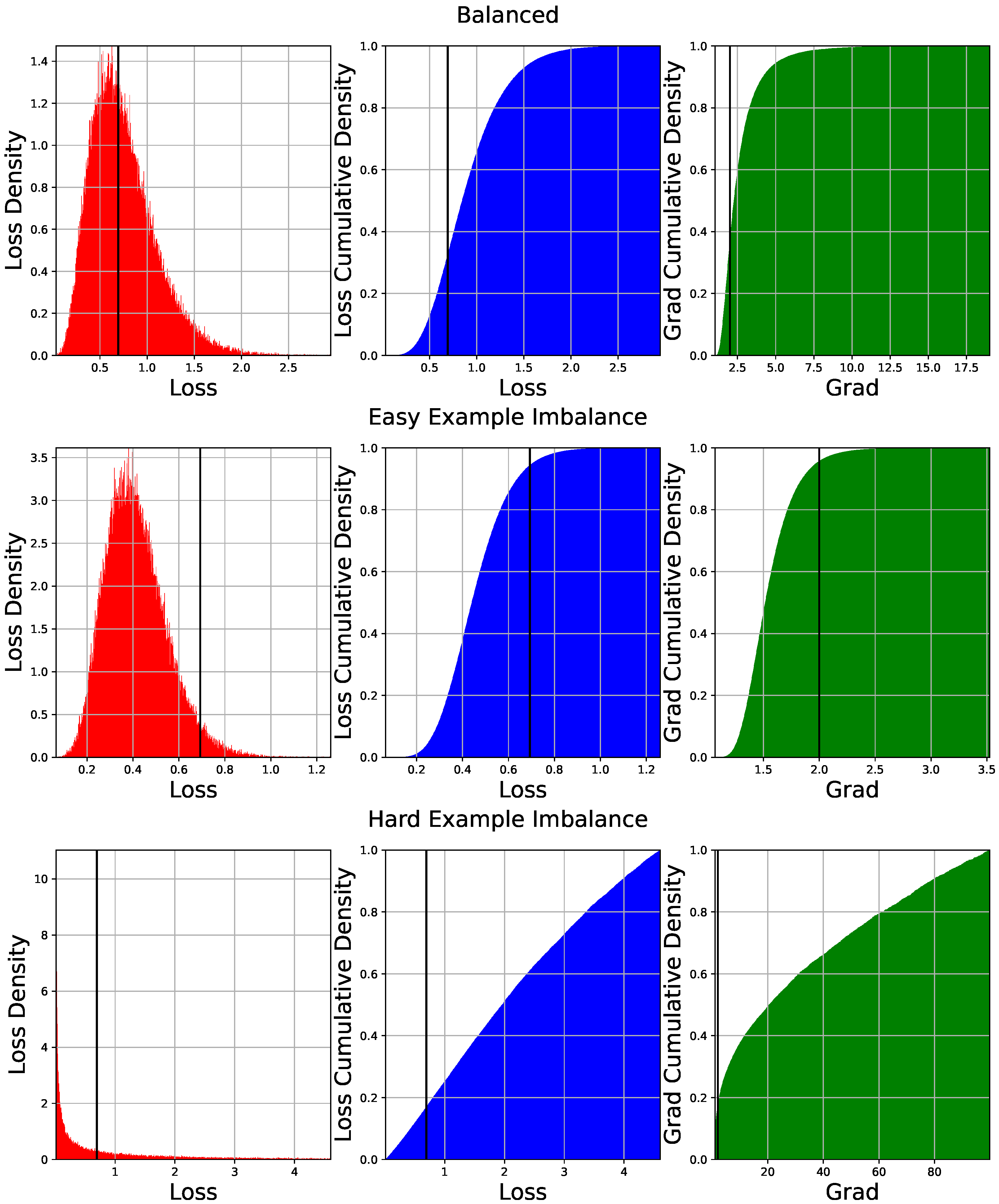
The formation and the harm of easy example imbalance and hard example imbalance are different. Figure 1 is a visualization of different situations that occurred at a certain time point in the training of U-Net by cross-entropy loss on the KolektorSDD2 dataset.

In most learning tasks, the majority are easy examples. Even if easy examples have a small loss value, the sum can still outweigh other examples due to its large quantity. For example, the second row of Figure 1 displays that when easy examples are the majority and very few hard examples exist, most of the loss value and the gradient is attributed to the easy examples. Other examples near the “critical” point have a minor influence. When easy examples altogether have a major contribution to the overall loss, the training is largely influenced by those easy examples on which the model has already been making correct predictions. Penalizing predictions on easy examples have zero improvement on segmentation accuracy.

On another hand, the hard example imbalance occurs on a few examples with a large loss value. The third row of Figure 1 demonstrates the consequence of having a small amount of hard examples that produce very high loss. Hard examples take up more than half of the loss value and the gradient. Although fitting hard examples have potential long-term benefit, there is a risk of over-fitting on noisy data. For example, the commonly used focal loss suppresses the influence of easy examples and amplifies the loss of hard examples. When the hard examples consists of noisy data, focal loss will lead to an instable training process. In addition, over-optimization on a small portion of examples provides little improvement on overall segmentation accuracy.

Intuitively, easy–hard example imbalance can be tackled by limiting the loss value of easy/hard examples within a reasonable range. Our solution is the truncated cross-entropy loss, which is detailed in Section 2.3.2.

2.2.3. Boundary Imbalance

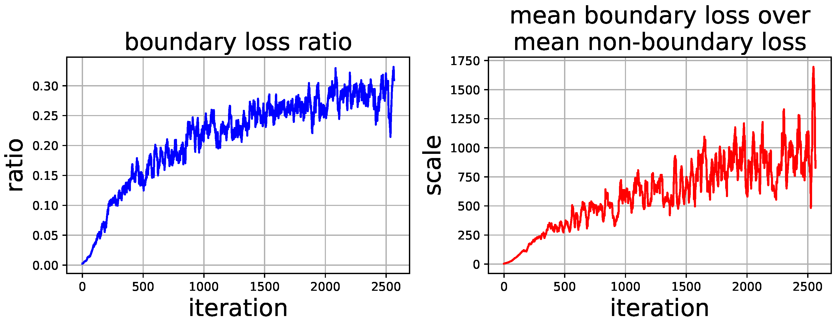
We observe boundary imbalance caused by label confusion in the training of surface defect segmentation models. We find that the points at the boundary of the defect, i.e., whose neighboring points have different labels from itself, constantly produce very large loss values compared with its small ratio in the image. Our experimental observation plotted in Figure 2 shows that points at the boundary of the defect can hold as much as 30% loss value, even if they are no more than 0.01% of all pixels. The loss of boundary points are hundreds (even more than one thousand) times the non-boundary points, and they do not converge in training.

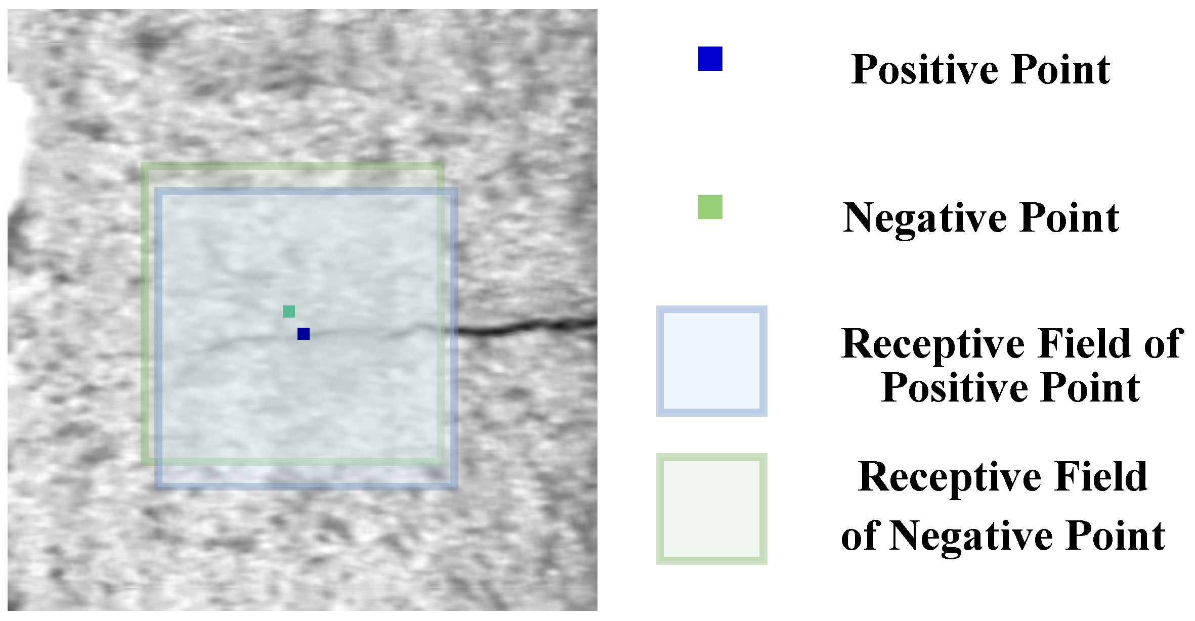
Our explanation to this phenomenon is label confusion. Figure 3 illustrates label confusion at the boundary. Each point-wise prediction of Y has a fixed receptive field associated with the neurons in CNN. For two neighboring points, their receptive fields almost completely overlap. Research [20] on CNN architecture shows that the neurons mainly focus on the features that lie at the center of their receptive field. Given almost the same feature input, the model is trained to make different predictions at the two sides of the label boundary. This makes boundary points naturally hard and noisy examples. Fitting these noisy examples can lead to over-fitting and impair the segmentation accuracy on other points.

The core of label confusion suppression is how to measure the degree of confusion. In Section 2.3.3, we propose an entropy-based method to suppress label confusion and avoid boundary imbalance of loss.

2.3. Balanced Loss Function

To address label imbalance, easy–hard example imbalance and boundary imbalance, respectively, we propose three strategies: dynamical class weighting, truncated cross-entropy loss and label confusion suppression. The three components are unified to work as a balanced loss function.

2.3.1. Dynamical Class Weighting

We address the label imbalance problem by a dynamical weighting scheme inspired by class-balanced loss proposed by Cui et al. [21]. Class-balanced loss aims to weigh class-specific loss by the number of effective examples. The class-balanced loss for classification is formulated as:

$$\begin{array}{c}\hfill {\mathcal{L}}_{CB}=-\frac{1-\beta }{1-{\beta }^{N_k}}log(1-ϵ)\end{array}$$

(1)

where $\beta \in (0,1)$ is a hyper-parameter, k is the label of the example, and $N_k$ is the occurrence of class k in the dataset. This class-balanced loss will assign higher weight to the loss of less-represented classes while training. Experiments in [21] show accuracy improvement on the class-imbalanced data of image classification problems.

In surface defect segmentation, the label imbalance problem exists at the pixel level. We adapt the class-balanced loss to a dynamical one by scaling loss values by pixel label distribution, which means $N_i$ in Equation (1) should represent the pixel number of a class. Assume that for the annotation A of an image, the label distribution is $\{N_1,N_2,\dots ,N_C\}$ that satisfies $N_1+N_2+\dots +N_C=W\ast H$. We define a pixel weighting mask $M_{class}$, whose value at point $(i,j)$(pixel label is k) is:

$$\begin{array}{c}\hfill M_{clas{s}_{i,j}}=\frac{1-\beta }{1-{\beta }^{N_k}}\end{array}$$

(2)

Our approach is different from the original class-balanced loss in several ways. First, it is no longer associated with cross-entropy loss or other loss functions; it is a soft mask over pixel-level loss values that performs weighting. Second, $N_k$ counts pixels rather than the images of a class. Last, unlike [21] where the hyper-parameter $\beta$ is selected based on dataset volume, we select $\beta$ by the image size $W\times H$. The experiments for the optimal selection of $\beta$ is provided in Section 3.

2.3.2. Truncated Cross-Entropy Loss

Most point-wise segmentation loss functions can be interpreted as the penalization on the point error $ϵ$ of probabilistic prediction $y\in (0,1)$ (an entry of Y) given the label $\widehat{y}\in \{0,1\}$ (an entry of $\widehat{Y}$):

$$ϵ=\left\{\begin{array}{cc}y,\hfill & \widehat{y}=0\hfill \\ 1-y,\hfill & \widehat{y}=1\hfill \end{array}\right.$$

(3)

The cross-entropy loss uses a logarithmic function to scale up the error:

$$\begin{array}{c}\hfill CE\left(ϵ\right)=-ln(1-ϵ)\end{array}$$

(4)

To scale down the loss value of easy and hard examples, we propose a truncated cross-entropy loss. First, an upper bound ${ϵ}_{sup}\in (0,1]$ and a lower bound ${ϵ}_{inf}\in [0,1)$ (satisfying ${ϵ}_{sup}>{ϵ}_{inf}$) are set to identify easy and hard examples. The truncated cross-entropy loss is defined as:

$$TruncCE\left(ϵ\right)=\left\{\begin{array}{c}0,ϵ<{ϵ}_{inf}\hfill \\ -ln(1-ϵ)-t_{inf},{ϵ}_{inf}\le ϵ\le {ϵ}_{sub}\hfill \\ \frac{ϵ-{ϵ}_{sub}}{1-{ϵ}_{sub}}+t_{sub}-t_{inf},{ϵ}_{sub}<ϵ\hfill \end{array}\right.$$

(5)

where

$$\begin{array}{c}\hfill t_{inf}=-ln(1-{ϵ}_{inf})\\ \hfill t_{sub}=-ln(1-{ϵ}_{sub})\end{array}$$

(6)

The truncated cross-entropy loss is a consistent piece-wise loss function with two non-differentiable points at $ϵ={ϵ}_{inf}$ and $ϵ={ϵ}_{sub}$. To make it compatible with gradient descent optimization, we set the derivative of the two singular points consistent with one side, and the derivative of the truncated cross-entropy function is formalized as:

$$\frac{dTruncCE\left(ϵ\right)}{dϵ}=\left\{\begin{array}{cc}0,\hfill & ϵ<{ϵ}_{inf}\hfill \\ \frac{1}{1-ϵ},\hfill & {ϵ}_{inf}\le ϵ\le {ϵ}_{sub}\hfill \\ \frac{1}{1-{ϵ}_{sub}},\hfill & {ϵ}_{sub}<ϵ\hfill \end{array}\right.$$

(7)

The derivative of the truncated cross-entropy loss is inconsistent, and the derivative is zero for easy examples ($ϵ<{ϵ}_{inf}$). Such properties can be found in many other classical loss functions. For example, mean absolute error (MAE) regression loss has an inconsistent point at $ϵ=0$; Huber loss has two singular points the separate easy and hard examples; Hinge loss also sets zero loss value and zero derivative for easy examples. In modern auto-gradient-based neural network implementations, the inconsistency and non-smoothness of the loss function on a few points can be tackled by user-specified gradient calculation.

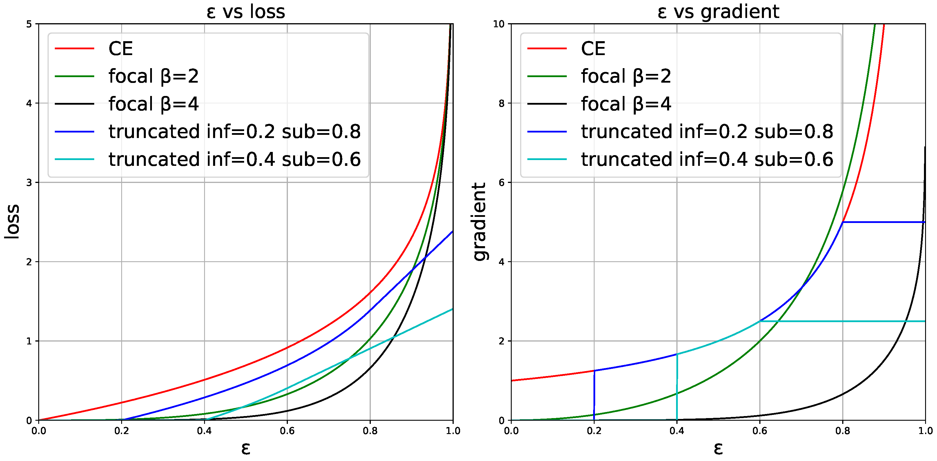
Figure 4 visualizes the loss value and the gradient over $ϵ$ of cross-entropy loss, focal loss and truncated cross-entropy loss. It throws light on how easy/hard examples are treated differently. For cross-entropy loss, the loss value and the gradient of easy examples (small $ϵ$) are still significantly large compared to difficult examples. Especially, when $ϵ$ is close to 0, cross-entropy loss still assigns gradient value 1 to the point, forcing the model to fit very easy examples. Considering that the quantity of easy examples is enormous, the loss will be dominated by them. Truncated loss function sets the loss value and gradient of easy examples to zero to suppress such imbalance. Focal loss scales down the loss and gradient of easy examples by a continuous means.

For hard examples, most loss functions produce a very large loss and gradient. For a better view, it is not plotted that cross-entropy and focal loss soar to $10.0+$ when $ϵ$ approaches $1.0$. The loss and gradient can probably be dominated by hard examples in certain phases of training. Although focal loss ($\beta =4$) seems to have relatively low gradients on hard examples, the gradients of other examples have already been suppressed. Truncated cross-entropy loss produces a constant gradient value for hard examples, allowing a balanced distribution of training focus on hard and not-very-hard examples.

2.3.3. Label Confusion Suppression

Our solution to the boundary imbalance problem has two steps: first, measure the level of label confusion at each point; then, suppress the loss of the points with label confusion.

We propose an entropy-based measurement of label confusion. Entropy is a commonly used measurement of distribution variance. The entropy (using a natural constant as the base) of a discrete random variable $X\in \{x_1,x_2,\dots ,x_N\}$ is:

$$\begin{array}{c}\hfill H\left(X\right)=-\sum _{i=1}^{N}P\left(x_i\right)lnP\left(x_i\right)\end{array}$$

(8)

We use the label entropy as the measurement of local region label confusion. For a $r\times r$ ($r>1$ and is odd) square region centered at point $(i,j)$ in pixel annotation A, which is denoted as $local\left(A_{i,j}\right)\in {\mathbb{N}}^{r\times r}$, the label entropy is:

$$\begin{array}{c}\hfill H\left(A_{i,j}\right)=-\sum _{k=1}^C\frac{N_{i,j,k}}{r^2}ln\left(\frac{N_{i,j,k}}{r^2}\right)\end{array}$$

(9)

where $N_{i,j,k}$ is the number of occurrence of label k within $local\left(A_{i,j}\right)$. The higher the label entropy, the more the label confusion at point $(i,j)$. The maximum of the label entropy is $ln\left(C\right)$.

To suppress the points with high label confusion, we calculate a soft mask $M_{confusion}\in {\mathbb{R}}^{W\times H}$ for loss computation, whose entries are:

$$\begin{array}{c}\hfill {M_{confusion}}_{i,j}=1-\frac{H\left(A_{i,j}\right)}{ln\left(C\right)}\end{array}$$

(10)

$M_{consufion}$ is defined as a constant soft mask over the loss values to suppress label confusion. The higher the label confusion, which is measured by Equation (9), the lower the weight given by Equation (10). When multiple labels mingle in a local region and confuse the training at $(i,j)$, the confusion mask will suppress the loss value and reduce the noise on the overall loss value. Section 2.3.4 introduces the connection between $M_{confusion}$ and other components.

2.3.4. The Unified Function

Figure 5 visualizes the pipeline of the balanced loss for segmentation. By truncated cross-entropy loss, an unbalanced loss $L_{unbalanced}$ is computed by prediction Y and annotation A (A is one-hot encoded into $\widehat{Y}$ before computation). Meanwhile, a dynamical class weighting mask $M_{class}$ and a label confusion suppression mask $M_{confusion}$ are computed from A. At last, the balanced loss $L_{balanced}$ is computed by the element-wise production of $L_{unbalanced}$, $M_{class}$ and $M_{confusion}$. The final loss value can either be the mean or sum of the entries of $L_{balanced}$.

In practice, because $M_{confusion}$ and $M_{class}$ do not depend on any runtime variable, they can be computed before training to avoid repeated computation in the training phase. What is more, because the computation of $L_{balanced}$ is the element-wise production of $L_{unbalanced}$, $M_{confusion}$ and $M_{class}$, the production can also be computed before training to save time. Our implementation shows that the computational speed of the balanced loss is very close the normal cross-entropy loss.

3. Experiments

3.1. Experiment Settings

Our experiments are performed on KolektorSDD2 [17], Severstal [18] and an original aluminum alloy surface defect dataset.

KolektorSDD2 consists of 7094 images collected and annotated by the Kolektor Group on different items from a visual inspection system. The main challenge with KolektorSDD2 is that the defect is tiny and rare. The images are of size $230\times 630$ pixels, but on average, the defect only contains 2.697% of all pixels. With a 1:9 positive/negative example ratio, the label imbalance problem is also challenging in KolektorSDD2.

Severstal is a steel sheet defect dataset released by the Severstal company. It is made of 12,538 training images and 5476 test images with four defect types and $1600\times 256$ resolution. Because the annotations for the test images are not officially released, we randomly split the training set into a 8727-image new training set and a 3811-image new test set, following the official splitting ratio. Defects are salient on the images, covering approximately 50% of the area on average, but the label imbalance between defect classes is large (see Table 2).

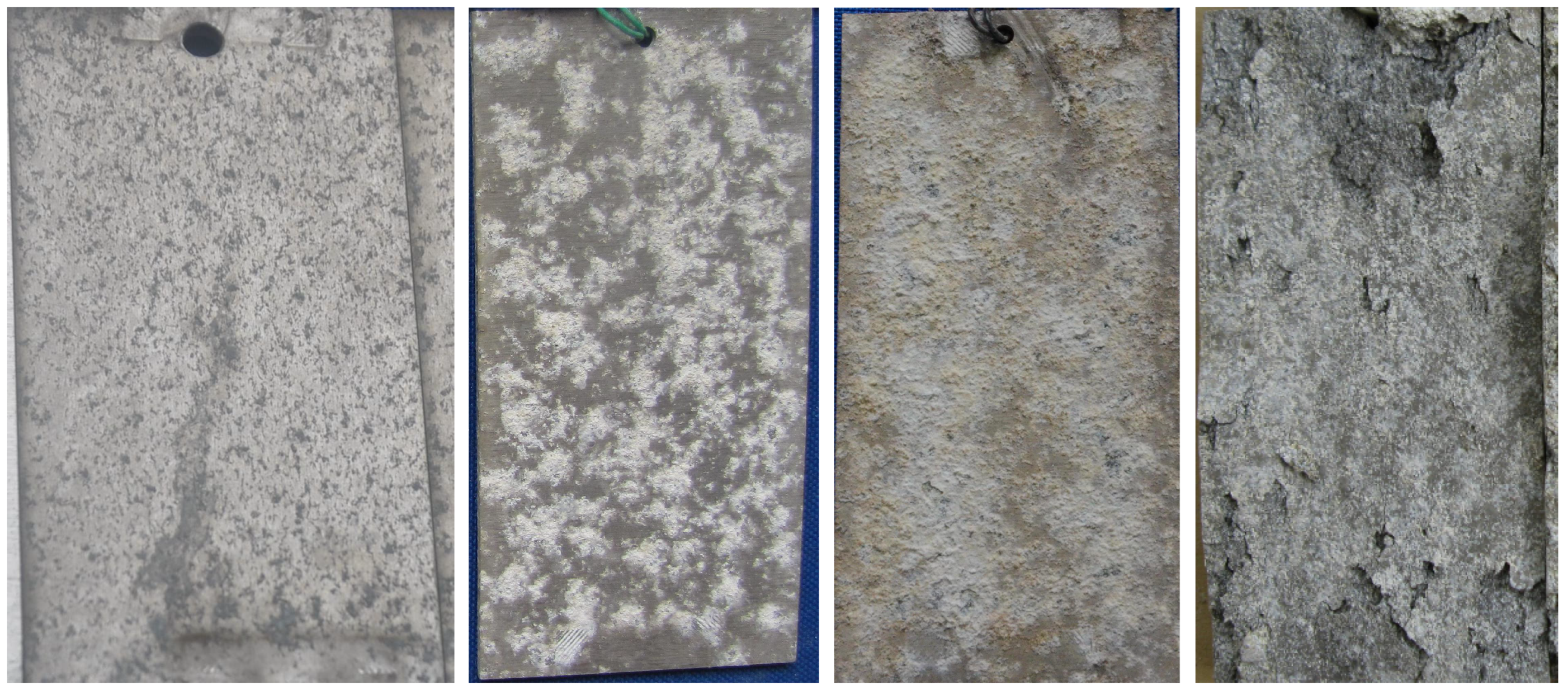
We collect 830 high-resolution images of aluminum alloy surface for benchmarking segmentation models. The images are acquired from the laboratory where aluminum alloy samples are processed in different environmental conditions to observe and analyze the corrosion on an aluminum alloy surface. The alloy sample RGB images are captured by a normal digital camera indoors on a blue background surface. The environment light is controlled by hand to avoid over-illumination. The samples are cropped from the image to leave out the blue background (but unavoidably, some images contain small background regions at the corner). The surface defects are labeled by proficient material chemistry researchers using an image annotation software to fill the regions with surface defects. Four types of defect are annotated, including corrosion spot, corrosion product, corrosion pit and chemical denudation (see examples in Figure 6). The statistics about the defect labels are in Table 2.

For the training of segmentation models, the images are further processed (cropping and resizing) as regularly sized $512\times 512$ images. We split the dataset into a 600-image training set and a 230-image test set. Pixel-level and image-level label imbalance both exist in this dataset.

The segmentation accuracy of models is evaluated by intersection-over-union (IoU). The image-wise class-specific IoU is computed for each defect type. The final class-specific IoU is the mean of image-wise class-specific IoU. We also report mean IoU (mIoU), which is the mean of all class-specific IoUs, as the overall metric of segmentation accuracy.

To verify that the balanced loss is effective for any segmentation models, we perform experiments on several popular segmentation networks: fully convolutional network (FCN) [22], U-Net [23], SegNet [24], DeepLabV3 [25] and pyramid scene parsing network (PSPNet) [26]. The selected models are representatives of different segmentation model architectures that are widely employed for surface defect segmentation. FCN and PSPNet are fully convolutional architectures that use an upsampling layer to increase feature map resolution. SegNet and U-Net are typical encoder–decoder architectures that have multiple upsampling or deconvolution layers. DeepLabV3 features an atrous spatial pyramid pooling module that extracts feature pyramids by dilated convolutional. For FCN and SegNet, the VGG16 backbone [27] is employed as encoders; for DeepLabV3 and PSPNet, the backbone is ResNet-50 [28]; U-Net has the original eight-convolution encoder/decoder design, with deconvolutional layers for up-sampling.

The models are trained with Adam optimizer [29] (learning rate ${10}^{-4}$, weight decay ${10}^{-6}$) and an exponential learning rate regularizer ($\gamma =0.995$). The training epoch number for KolektorSDD2, Severstal and the aluminum alloy dataset are 100, 50 and 100, respectively. Data augmentation techniques are used for all training, including random flipping, random rotation and random color jittering. We do not blur or sharpen the images because the defect can be very tiny and sensitive to such transformations.

The balanced loss is compared with other loss functions as counterparts, including cross-entropy loss (CE), weighted cross-entropy loss (WCE), focal loss (FL), Dice loss (Dice), inverse weighting loss (iw) [13] and Lovász loss [30]. For WCE, the weight of positive/negative examples is set according to image-level label imbalance. For example, there are about nine times as many negative images as positive images in KolektorSDD2 (see Table 2), so the positive class loss weight is 9 in WCE and 1 for negative class loss. For focal loss, we use the same rule to set $\alpha$. $\beta$ is set to 2 or 4 (both cases are evaluated).

In comparative experiments, the hyper-parameters of the balanced loss are chosen empirically. For dynamical class weighting, the scaling factor $\beta$ is $0.99$; for truncated cross-entropy loss, the two thresholds are ${ϵ}_{inf}=0.3$ and ${ϵ}_{sub}=0.7$. For label confusion suppression, the size of the neighboring region is $r=7$. The sensitivity to the hyper-parameters is tested in the experiments.

3.2. Quantitative Evaluations

3.2.1. KolektorSDD2

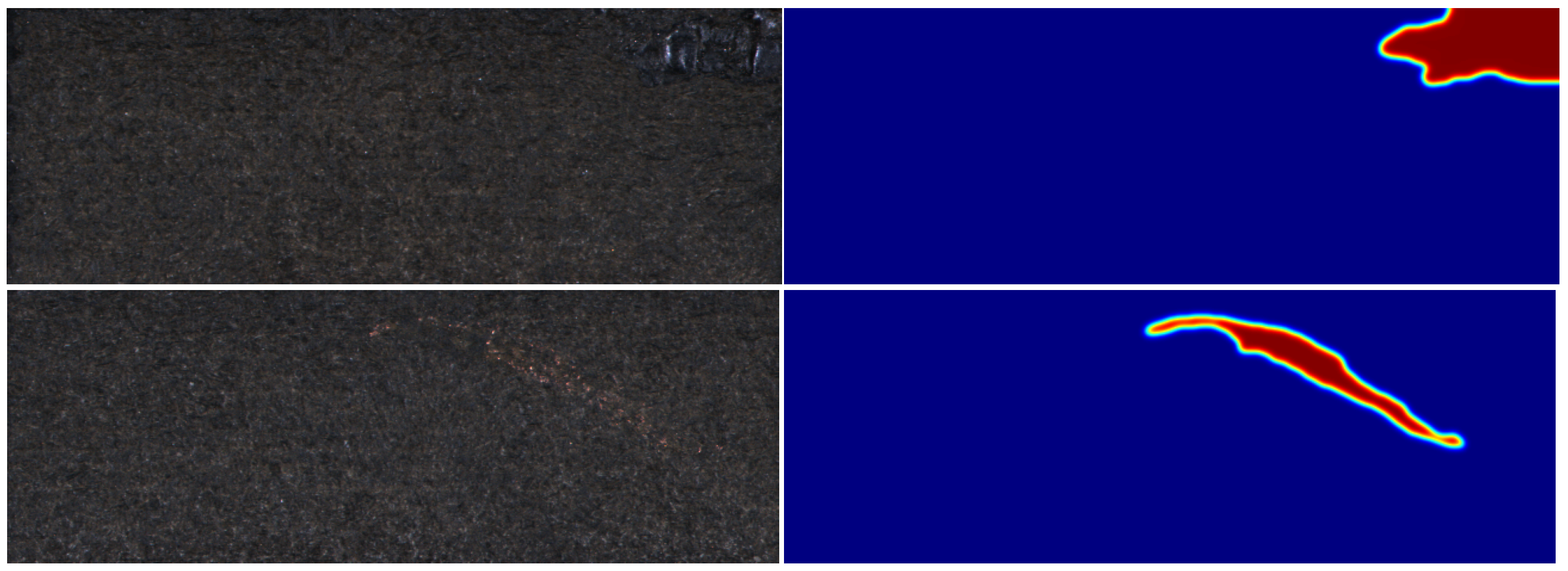
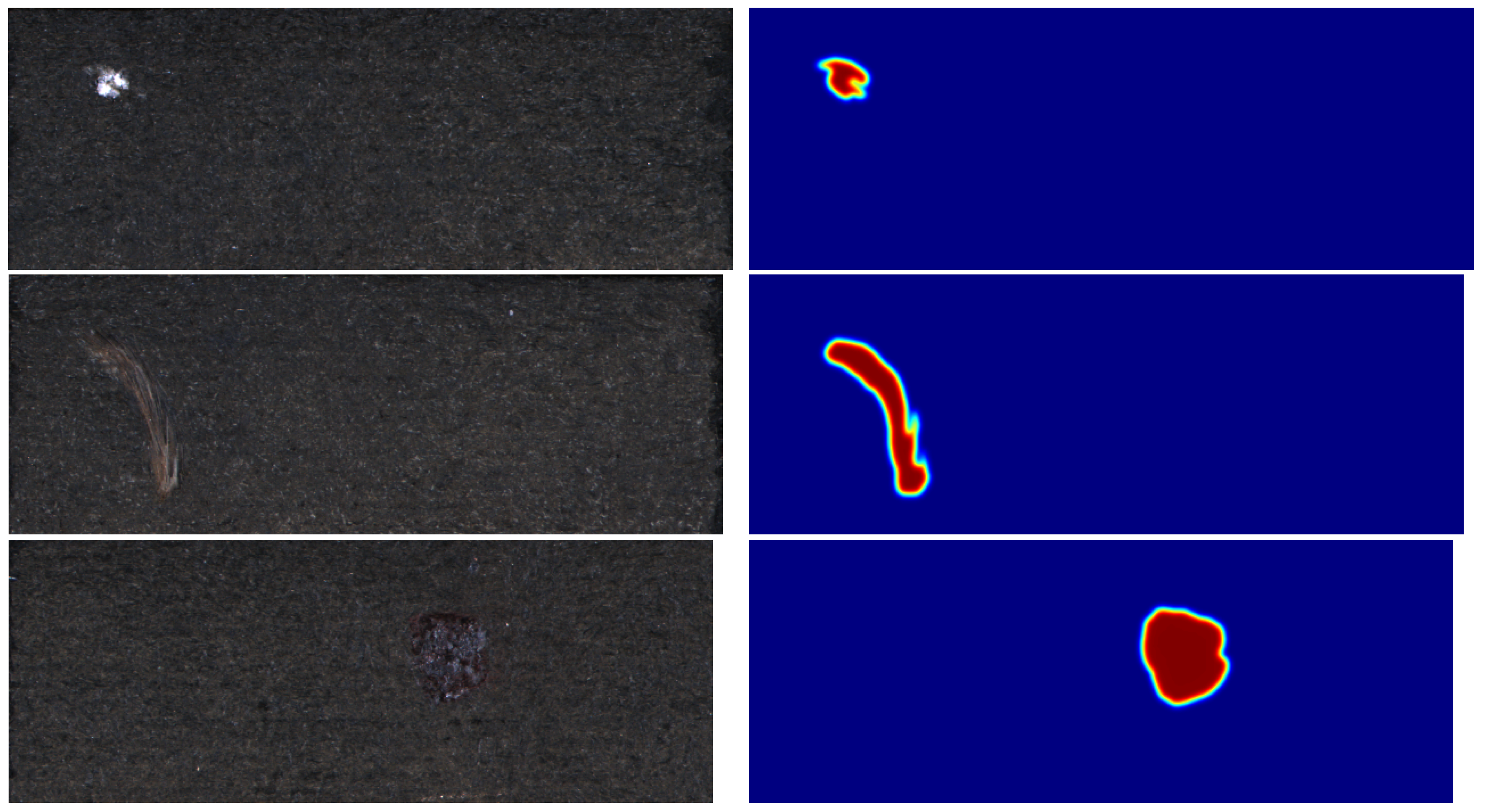
Figure 7 presents a comparison of the performance of loss functions conditioned on different networks trained on KolektorSDD2. The balanced loss significantly outperforms other loss functions in all networks, surpassing the second best by 18% at most and 10% at least. The experiment also reveals that region-based loss (Dice loss and Lovasz loss) is also advantageous over other pixel-based loss functions, because the pixel label imbalance problem is mitigated in Dice loss by Dice coefficient computation. However, our balanced loss succeeds to ease label imbalance in a pixel-based manner, retaining the room for solving other imbalance problems. Featuring online hard example mining, focal loss has some improvement on the basic cross-entropy loss. However, focusing on hard examples, which are possible noisy or invaluable examples, does not turn out to be a good strategy in KolektorSDD2. These findings can be consistently observed across all networks. Figure 8 presents visualized semantic segmentation results of KolektorSDD2 defect examples.

3.2.2. Severstal

We report the segmentation performance of different networks trained by the balanced loss and other counterparts in Figure 9. Most of our findings in KolektorSDD2 are still true in Severstal. The balanced loss outperforms other functions significantly. However, Dice loss or focal loss only has marginally advantageous CE and WCE. What makes this difference from the results on KolektorSDD2 is that Severstal has more salient (about 50% of the image area on average) and more contiguous defects. The training is less influenced by hard examples and the weaker label imbalance, which reduce the advantage of Dice loss and focal loss. For the same reason, skip-connection equipped networks (U-Net and DeepLabV3) have less advantage over others. Because the defects are salient, the model needs large context information to make point predictions. Figure 10 shows segmentation predictions on test examples of Severstal.

To analyze the impact of label imbalance on the model, the class-wise IoU of trained U-Net is presented in

Table 3. Class-wise IoU and mIoU of U-Net trained on Steveral with different loss functions.

Method	Cls1	Cls2	Cls3	Cls4	mIOU
CE	0.72	0.42	0.76	0.69	0.65
WCE	0.60	0.44	0.75	0.59	0.59
Focal $\beta =2$	0.68	0.61	0.82	0.69	0.70
Focal $\beta =4$	0.78	0.63	0.80	0.79	0.75
Dice	0.67	0.59	0.82	0.67	0.69
Balanced Loss	0.82	0.76	0.95	0.89	0.87

. Classes with more instances, such as defect type class 3 that appears on 72.58% images, tend to have better segmentation accuracy, while the accuracy on less represented classes, e.g., class 2 of 3.481% images, is worse. However, the balanced loss achieves significantly higher performance on class 2, and it displays the effectiveness of the balanced loss on solving label imbalance problems. In addition to class 2, others classes show minor improvement from using focal loss or Dice loss. The result suggests that using focal loss or Dice loss for the segmentation of a salient surface defect is not very effective.

The sensitivity of the hyper-parameters of the balanced loss function is reported in

Table 4. Mean IoU of U-Net trained on Steveral with varying truncated cross-entropy loss thresholds $\Delta ϵ$ and class weighting factor $\beta$.

Truncated CE Δ$\mathit{ϵ}$	$\mathit{\beta }$ Class Weighting
	0.0	0.9	0.99	0.999
0.1	0.73	0.73	0.82	0.79
0.2	0.70	0.70	0.87	0.86
0.3	0.70	0.69	0.86	0.83
0.4	0.69	0.70	0.78	0.79
0.5	0.60	0.62	0.65	0.65

. The $\beta$ factor of dynamical class weighting varies in $\{0.0,0.9,0.99,0.999\}$. When $\beta =0$, the weight is always $1.0$ (see Equation (1)), and $M_{class}$ is ineffective. In this experiment, the interval $[{ϵ}_{inf},{ϵ}_{sub}]$ of the truncated cross-entropy loss (Equation (5)) always has 0.5 as the center. Only one variable $\Delta ϵ\in (0,0.5]$ will decide the interval by letting ${ϵ}_{inf}=0.5-\Delta ϵ$ and ${ϵ}_{sup}=0.5+\Delta ϵ$. When $\Delta ϵ=0.5$, the interval is $[0,1]$, and the truncated cross-entropy loss degenerates to the normal cross-entropy loss.

The result shows that the optimal choice of $\beta$ is 0.99. For $\beta =0.9$, the performance approximately equals that of $\beta =0$. When $\beta =0.9$, we find that the values of $M_{class}$ are still very close to 1, which makes little difference from $\beta =0$. However, when $\beta =0.99$, the values of $M_{class}$ become 6 to 20 for imbalanced classes, and the weighting is appropriate in this task. Enlarging $\beta$ to 0.999 can impair the performance, because the imbalanced classes are over-weighted. $\Delta ϵ$ provides the good performance when it is at 0.2. However, the change of $\Delta ϵ$ from 0.1 to 0.4 does not cause a significant change in segmentation performance. Only the inactivation of the truncated cross-entropy loss ($\Delta ϵ=0$) will largely influence the performance. Considering that easy and hard examples mainly lie near $ϵ=0$ and $ϵ=1$, respectively, we believe that the truncated cross-entropy loss is most effective on these extreme examples.

3.2.3. Aluminum Alloy Surface Defect

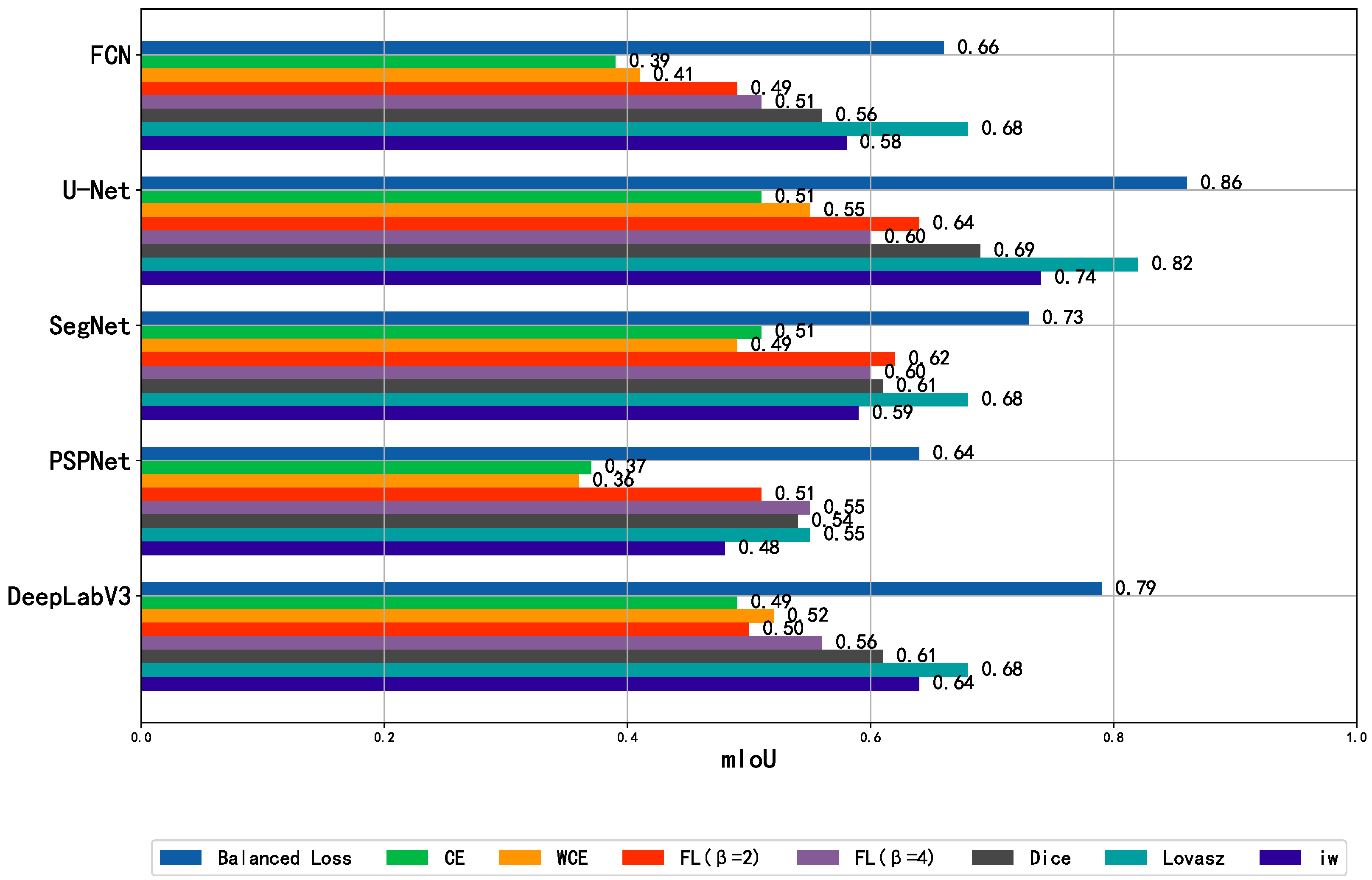
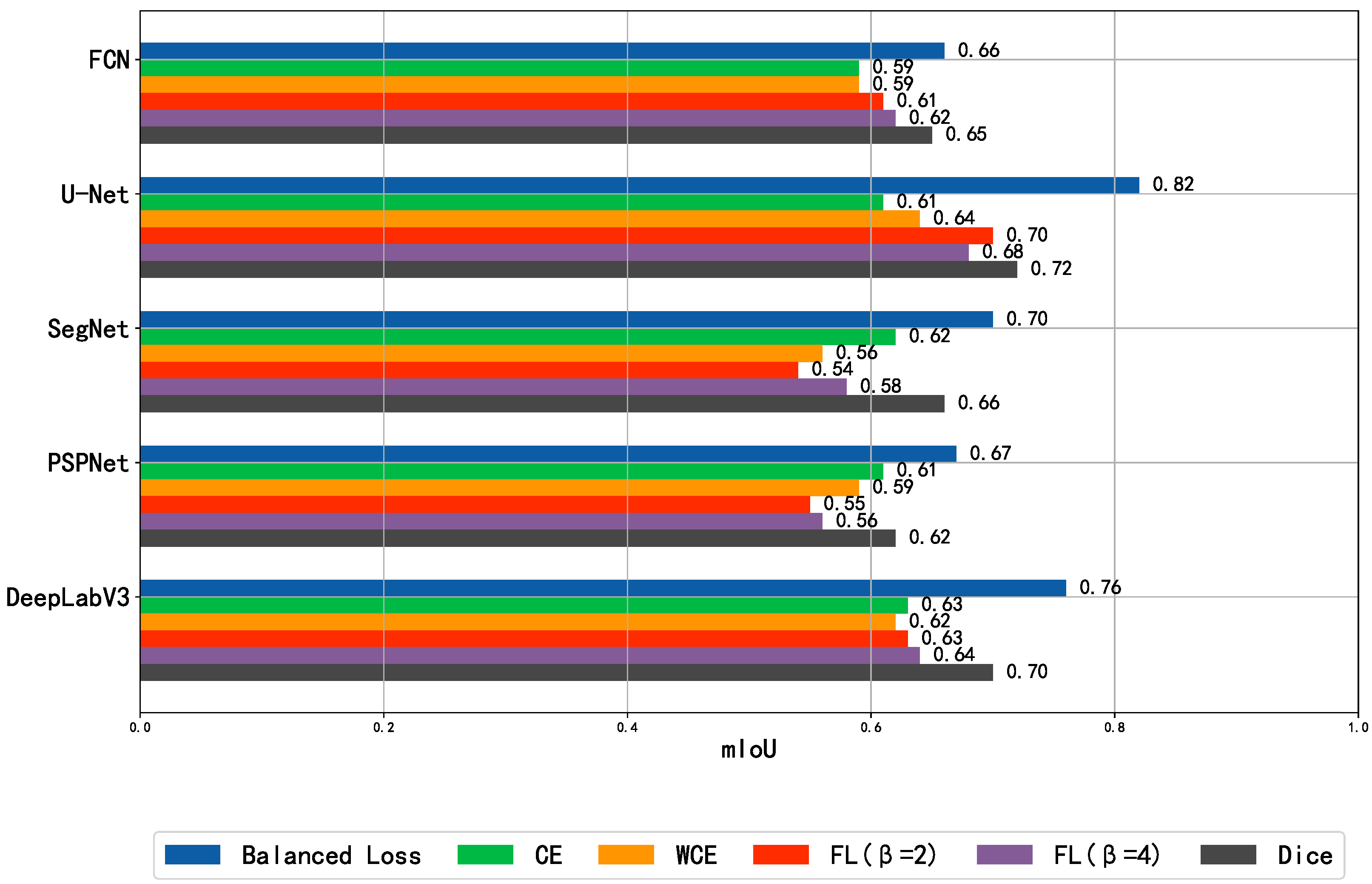
The segmentation accuracy of networks trained on the aluminum alloy surface defect dataset with different loss functions is presented in Figure 11. The balanced loss still shows a major promotion of accuracy. Other aspects of the results are similar to those of Severstal.

The class-wise IoU in

Table 5. Class-wise IoU and mIoU of U-Net trained on aluminum alloy surface defect dataset with different loss functions.

Method	Spot	Pit	Product	Denudation	mIOU
CE	0.45	0.41	0.71	0.88	0.61
WCE	0.43	0.46	0.73	0.87	0.64
Focal ($\beta =2$)	0.57	0.62	0.72	0.90	0.70
Focal ($\beta =4$)	0.53	0.59	0.70	0.90	0.68
Dice	0.57	0.62	0.80	0.89	0.72
Balanced (ours)	0.69	0.80	0.87	0.91	0.82

demonstrates the effectiveness of the balanced loss on solving pixel-level label imbalance. As we report in Section 3.1, corrosion spots are very tiny defects (3% image area on average), while usually, chemical denudation contains 89% of an image area on average. This label imbalance makes misprediction on corrosion spots very impactful. The results of the balanced loss on corrosion spots, corrosion pits, and corrosion products are improved by 12%, 18% and 7%. For chemical denudation, which is very salient, the performance is close to other loss functions. We also experiment on the sensitivity of hyper-parameters on the aluminum alloy surface defect dataset. The conclusion is consistent with that of Severstal except that the gap between $\beta =0.5$ and the others is not as huge as the gap in Table 4, which suggests this task is less threatened by easy–hard example imbalance. The sensitivity of the hyper-parameters of the balanced loss function is tested on this dataset, by the same approach as the experiment with Severstal. The result is presented in

Table 6. Mean IoU of U-Net trained on aluminum alloy surface defect dataset with varying truncated cross-entropy loss thresholds $\Delta ϵ$ and class weighting factor $\beta$.

Truncated CE Δ$\mathit{ϵ}$	$\mathit{\beta }$ Class Weighting
	0.0	0.9	0.99	0.999
0.1	0.63	0.72	0.80	0.76
0.2	0.70	0.78	0.82	0.79
0.3	0.68	0.75	0.81	0.76
0.4	0.68	0.73	0.79	0.75
0.5	0.65	0.65	0.70	0.68

.

3.3. Discussion

Experiments show that the proposed balanced loss has superiority in the training of surface defect segmentation models, especially in comparison with other point-wise loss functions CE, WCE and focal loss. The ablation experiment (Table 4) shows that dynamical class weighting and the truncated cross-entropy loss have significant contributions to the performance. In addition, the balanced loss exhibits its advantage on tiny defects, for example the spot and pit in Table 5. Region-based loss functions (Dice loss, inverse weighting loss and Lovasz loss) also show competitive performance. Unifying the merits of region-based loss functions and the balancing mechanisms of the balanced loss is an intriguing future research direction.

As for the segmentation models, networks with skip connections between the encoder (feature extractor) and the decoder (up-sampling modules), including U-Net and DeepLabV3, have better performance with the balanced loss. The recognition of surface defects is mainly dependent on a limited region of features at the center of the receptive field, which is very different from natural scene objects that have important context clues. Considering this fact, networks that link the output and low-level feature maps have a shortcut to efficiently exploit local features.

4. Conclusions

In this paper, we investigate and address the loss imbalance problem, which is one of the central problems with surface defect segmentation. We propose a balanced loss function which unifies three techniques, dynamical class weighting, truncated cross-entropy loss and label confusion suppression, to tackle the loss imbalance caused by imbalanced labels, easy-hard examples, and boundary points, respectively. In comparison with other counterpart loss functions, our experiment result shows the advantage of the balanced loss on the surface defect segmentation mean IoU, which surpasses other baselines by 5% to 30%.

However, the loss imbalance problem is inherent with DCNN segmentation models with pixel-wise dense predictions. The balanced loss function is only a domain-specific mitigation technique in surface defect segmentation. A generic solution to the loss imbalance problem will need further research in other semantic segmentation tasks, especially other causes of the loss imbalance problem, as well as improvements on the modeling paradigm and the optimization algorithm. A possible way to improve the loss function is to unify the merits of the balanced loss and region-based loss, such as Dice loss and Lovasz loss.