Optimal Lane Change Path Planning Based on the NSGA-II and TOPSIS Algorithms

Abstract

Among so many autonomous driving technologies, autonomous lane changing is an important application scenario, which has been gaining increasing amounts of attention from both industry and academic communities because it can effectively reduce traffic congestion and improve road safety. However, most of the existing researchers transform the multi-objective optimization problem of lane changing trajectory into a single objective problem, but how to determine the weight of the objective function is relatively fuzzy. Therefore, an optimization method based on the combination of the Non-Dominated Sorting Genetic Algorithm II (NSGA-II) and the Technique for Order Preference by Similarity to Ideal Solution (TOPSIS), which provides a new idea for solving the multi-objective optimization problem of lane change trajectory algorithm, is proposed in this paper. Firstly, considering the constraints of lane changing and combining with the collision detection algorithm, the feasible lane changing trajectory cluster is obtained based on the quintic polynomial. In order to ensure the comfort, stability and high efficiency of the lane changing process, the NSGA-II Algorithm is used to optimize the longitudinal displacement and time of lane changing. The continuous ordered weighted averaging (COWA) operator is introduced to calculate the weights of three objective optimization functions. Finally, the TOPSIS Algorithm is applied to obtain the optimal lane change trajectory. The simulations are conducted, and the results demonstrate that the proposed method can generate a satisfactory trajectory for automatic lane changing actions.

1. Introduction

1.1. Motivation

According to statistics from the National Highway Traffic Safety Administration, from 2020 to 2021, estimated crashes caused by motor vehicles increased 11.25 percent from 2,425,374 to 2,698,338 [1]. Traffic safety is always the top priority when traveling [2]. In addition, about 94% of traffic accidents are caused by drivers’ own reasons, such as lack of concentration and fatigue driving [3], of which accidents caused by lane changing behavior account for 4% to 10% [4]. Intelligent transportation systems, especially autonomous driving technology, are regarded as an effective solution to deal with the complex traffic environments in the future and have attracted widespread attention from people in all walks of life. It can relieve traffic pressure and reduce traffic accidents. At present, the research and development of autonomous driving technology is widely carried out in academia and industry [5,6,7,8,9], mainly involving decision making, planning and control. Among them, intelligent vehicle autonomous lane changing is an important application scenario, and it is also one of the links to traffic behaviors such as overtaking and U-turns [10], which have become a current research hotspot. Compared with the lane keeping system, the autonomous lane changing system is mainly used in a more complex dynamic environment, which needs to consider the surrounding environment facilities and other vehicles, and the conditions are more severe. These include wrong lane changing decisions, unreasonable path planning or invalid control algorithms that have the potential to cause traffic jams or even traffic accidents [11]. A complete autonomous lane changing system can be divided into four parts: perception and communication module, lane change decision module, path planning module and trajectory tracking module [12]. The in-vehicle communication system can make up for the shortcomings of the sensor itself. Through wireless communication modes, such as V2I and V2V, autonomous vehicles can obtain more real-time traffic data to optimize their driving strategies [13,14]. In addition, 5G will further enhance the V2X information interaction capability, making communication more convenient and faster [15]. The purpose of lane changing decision making is to determine when to change lanes. During the lane changing process, vehicles should ensure safe driving and not collide with surrounding facilities and vehicles. When there is a risk in lane changing, the lane changing behavior should be stopped immediately [16,17]. The path planning module comprehensively considers factors, such as obstacle avoidance, stability constraints, lane changing efficiency, etc., and plans the optimal lane changing curve according to the real-time traffic environment. The path planning module acts as a bridge between decision making and trajectory tracking control modules. The planned lane changing trajectory after receiving the lane changing command issued by the decision-making module will directly affect the accuracy of trajectory tracking and passenger comfort. The trajectory tracking module calculates the vehicle’s turning angle, driving force (throttle valve opening), etc., as input through the lateral and longitudinal displacement, speed, curvature, and other information of the planned path so that the vehicle can follow the planned path as precisely as possible [5].

1.2. Literature Review

As the core part of the autonomous lane changing system, path planning is the key to ensuring safe driving. Many scholars have conducted a lot of fruitful research. The following highlights some of the research results.

Jhanani Selvakumar et al. proposed a CC-RRT* Algorithm for autonomous vehicle lane changing in high-speed scenarios [18]. The algorithm based on curve interpolation is the most widely used path planning algorithm for autonomous lane changing of intelligent vehicles. The planned path is usually described in the form of a mathematical function. Different path curves can be obtained by adjusting parameters, such as time and curvature. This method can consider the kinematics and dynamics of the vehicle and can be used for obstacle avoidance in dynamic environments to obtain a safe, stable, and easy-to-track lane changing path curve. The trajectory generated by the lane change trajectory algorithm proposed by Li Bae et al. based on the curvature of Bezier curve can be used to estimate the maximum lateral acceleration [19]. Dequan Zeng et al. proposed a method combining a B-spline curve and RRT to plan the lane changing path and monitor the trajectory at the same time to ensure the robustness of the algorithm. However, when the traffic environment is complex, the success rate of generating the lane changing path will decrease [20]. Zhiyuan Li et al. established a second-order continuous quintic spline curve in the Frenet coordinate system, taking into account the curvature and heading angle of the planned path to ensure the safety and stability of the vehicle during the lane change process [21]. In order to obtain an algorithm suitable for autonomous lane change, Armin Norouzi et al. compared the quintic polynomial function, the sine function, and the tangent function according to the RMS value of peak acceleration and finally chose the quintic polynomial as the lane changing model [22]. Based on the unconstrained lane changing trajectory cluster generated by the quintic polynomial, Haijian Bai et al. obtained the feasible lane changing trajectory cluster through vehicle kinematics constraints and comfort requirements and finally determined the optimal lane changing trajectory through the cost function, realizing the safety and stability of the lane changing process [23]. Chenyang Xi et al. applied deep learning and data-driven methods to polynomial lane changing trajectory optimization so that the final lane changing trajectory followed traffic rules [24]. In recent years, V2V technology has been widely used in autonomous driving. Yong Xiang et al. proposed a dynamic autonomous lane changing system based on V2V, which is updated during the lane changing process to avoid possible collision behavior, and uses the lane changing time and distance to transform the planning problem into a constrained optimization problem so that the planned reference trajectories meet safety, comfort, and traffic efficiency requirements [25]. Yonggang Liu et al. established a path planning model and a speed planning model through cubic polynomial interpolation based on the local trajectory generated by GPS and proposed a comprehensive trajectory optimization function to ensure driving safety, passenger comfort, and lane changing efficiency [2]. N.A. Othman et al. proposed a Hermite interpolation algorithm, which can determine the maximum speed of safe driving through the curvature information of the generated path [26]. WANG Jiang Feng characterizes lane changing trajectory by combining a linear function and a sine function [27]. Bangjun Qiao et al. obtained the optimal lane changing path, taking into account safety and comfort through a quadratic programming algorithm [28]. Zhaolun Li et al. combined the bicycle model with the function of automatically determining the target lane and realized the autonomous lane changing of vehicles in the dynamic environment through the model predictive control method (MPC) [29]. Nobuto Sugie et al. regard vehicle dynamics, physical constraints, and safety requirements as constraints, proposed a synchronous planning and control framework based on nonlinear model predictive control, and applied it to lane changing tasks [30]. Hong Wang et al. proposed an LSTM-MPC algorithm to predict the trajectory of surrounding vehicles through an LSTM network training data set to realize safe lane changing [31].

The many alternate path planning algorithms mentioned above can generally be divided into two categories: numerical-optimization-based and sampling-based. The method based on numerical optimization can simultaneously consider the constraints of the ego vehicle and the surrounding environment. Due to the non-convexity of most path planning, optimization problems are difficult to solve. Sampling-based methods generally have the ability to generate a large number of high-quality candidate paths. A random sampling method can be used to generate a lane change path quickly, but the smoothness of the path is often unusable and may not be optimal.

To the authors’ knowledge, only a few research findings account for the optimization problem of two or even more variables. In addition, the determination of cost function weight in existing references is relatively fuzzy. To solve the issue mentioned above, an algorithm based on NSGA-II and TOPSIS is proposed in this paper, which is convenient for solving the multi-objective optimization problem in the lane change process quickly. It not only retains sufficient reference trajectory, but also considers the constraints, making the lane change trajectory smooth and continuous.

In fact, a genetic algorithm is widely used to solve optimization problems, but few scholars have applied it to lane change path planning. NSGA-II is able to find a much better spread of solutions and better convergence near the true Pareto-optimal front compared to the Pareto-archived evolution strategy and the strength-Pareto Evolutionary Algorithm—two other elitist multi-objective evolutionary algorithms that pay special attention to creating a diverse Pareto-optimal front. While comparable to NSGA, the time complexity of NSGA-II is greatly reduced due to the adoption of fast non-dominated sorting and elite strategy.

2. Optimal Lane Change Path Planning Based on the NSGA-II and TOPSIS Algorithms

This section optimizes the lane change trajectory based on the NSGA-II Algorithm to obtain the Pareto optimal solution set. On this basis, COWA operator is introduced to calculate the weight of the evaluation indicators of the three objective optimization functions. Finally, the TOPSIS Algorithm is applied to evaluate and sort the solutions in the Pareto optimal solution set to obtain the optimal lane change path.

2.1. Lane Change Trajectory Based on Polynomials

In order to ensure that the velocity, acceleration, and curvature of the lane change trajectory are continuous and bounded and at the same time meet the boundary conditions at the beginning and end of the lane change, the lane change trajectory based on the quintic polynomial is adopted in this section, which can be expressed as:

$$\{\begin{array}{l}x\left(t\right)=a_0+a_{1}t+a_2{t}^2+a_3{t}^3+a_4{t}^4+a_5{t}^5\\ y\left(x\right)=b_0+b_{1}x+b_2{x}^2+b_3{x}^3+b_4{x}^4+b_5{x}^5\end{array}$$

(1)

where, $a_i,b_i\left(i=1,2\cdots 5\right)$ are coefficients to be determined. At the initial time $t_0$ and the end time $t_f$ of the lane changing, the longitudinal and lateral lane change boundary conditions meet Equations (2) and (3), respectively,

$$\{\begin{array}{l}x\left(t_0\right)=0,\dot{x}\left(t_0\right)=v_0,\ddot{x}\left(t_0\right)=0\\ x\left(t_f\right)=x_f,\dot{x}\left(t_f\right)=v_f,\ddot{x}\left(t_f\right)=0\end{array}$$

(2)

$$\{\begin{array}{l}y\left(x_0\right)=0,\dot{y}\left(x_0\right)=0,\ddot{y}\left(x_0\right)=0\\ y\left(x_f\right)=w,\dot{y}\left(x_f\right)=0,\ddot{y}\left(x_f\right)=0\end{array}$$

(3)

In Equations (2) and (3), each state parameter and its definition are shown in Table 1. In order to simplify the calculation, $t_0=0,w=3.75m$ are set in this study, in which $w$ is the lateral displacement of lane changing, that is, the lane width. Longitudinal displacement $\Delta x=x_f$ and lane change time $\Delta t=t_f$ are variables that need to be optimized by the NSGA-II Algorithm.

Table 1. State parameters with their definitions.

State Parameters	Definition
$x\left(t_0\right)$	The longitudinal coordinate of the ego vehicle at the beginning of the lane changing
$\dot{x}\left(t_0\right)$	The longitudinal velocity of the ego vehicle at the beginning of the lane changing
$\ddot{x}\left(t_0\right)$	The longitudinal acceleration of the ego vehicle at the beginning of the lane changing
$x\left(t_f\right)$	The longitudinal coordinate of the ego vehicle at the end of the lane changing
$\dot{x}\left(t_f\right)$	The longitudinal velocity of the ego vehicle at the end of the lane changing
$\ddot{x}\left(t_f\right)$	The longitudinal acceleration of the ego vehicle at the end of the lane changing
$y\left(x_0\right)$	The lateral coordinate of the ego vehicle at the beginning of the lane changing
$\dot{y}\left(x_0\right)$	The lateral velocity of the ego vehicle at the beginning of the lane changing
$\ddot{y}\left(x_0\right)$	The lateral acceleration of the ego vehicle at the beginning of the lane changing
$y\left(x_f\right)$	The lateral coordinate of the ego vehicle at the end of the lane changing
$\dot{y}\left(x_f\right)$	The lateral velocity of the ego vehicle at the end of the lane changing
$\ddot{y}\left(x_f\right)$	The lateral acceleration of the ego vehicle at the end of the lane changing

Through the lane changing boundary conditions in Equations (2) and (3), the quintic polynomial lane changing trajectory can be obtained. Assuming that the size of the ego vehicle and the surrounding traffic vehicles are the same, with a length of 4.2 m and a width of 1.82 m, the lane changing scene is as follows: The velocity of the ego vehicle is 50 km/h at the beginning of the lane change and 60 km/h at the end of the lane change. The velocity of the vehicle ahead in the current lane is 50 km/h, and the distance from the ego vehicle is 30 m. The velocity of the vehicle in front of the target lane is 60 km/h, and the distance from the ego vehicle is 50 m. The velocity of the vehicle behind the target lane is 55 km/h, and the distance from the ego vehicle is 30 m. The schematic diagram of the lane changing process is shown in Figure 1.

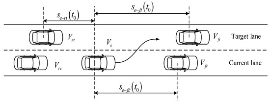
Figure 1. Schematic diagram of vehicle lane change.

According to the experience, the lane change time $\Delta t$ was selected as 4~8 s, and the longitudinal displacement of lane change $\Delta x$ was 60~135 m, in which the lane change time was 0.2 s as the simulation step and the longitudinal displacement was 2 m as the simulation step for the simulation experiment. The unconstrained lane changing trajectory cluster is obtained, as shown in Figure 2.

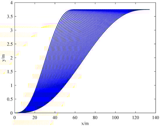
Figure 2. Unconstrained lane changing trajectory cluster.

2.1.1. Lane Change Trajectory Constraints

In the cluster of unconstrained lane changing trajectories, some cannot meet the feasibility requirements. Considering the dynamic constraints of the ego vehicle and the requirements of riding comfort, the constraint conditions of lane changing trajectories considered in this paper are as follows [32,33]:

(1)

Lateral displacement constraint: $0<y\left(t\right)<width$.

(2)

Security constraints: During the lane changing process, the ego vehicle does not collide with the surrounding traffic vehicle;, that is, the collision avoidance algorithm in Section 2.2 is satisfied.

(3)

Minimum lane change time constraint:

$$t_{\min }=2.745-2.997\mu +0.01093v+1.138{\mu }^2+0.0004618\mu v-3.107\times {10}^{-5}{v}^2$$

(4)

where $t_{\min }$ is the shortest time for the ego vehicle to change lanes smoothly, $\mu$ is the road adhesion coefficient, and $v$ is the speed of the ego vehicle. In this study, all the vehicles are assumed to be driving on an asphalt road, and the reference value of $\mu$ is 0.85.

(4)

Limited by the constraints between the tire and the road, the maximum lateral acceleration is $a_{y,\max }=\mu g$.

2.2. Collision Avoidance Algorithm

In order to avoid traffic accidents, the vehicle should ensure that there is enough safe distance with the surrounding vehicles when changing lanes. Hossein Jula et al. realized obstacle avoidance by calculating the safe distance to meet the lane change requirements [34]. Zhou Jian et al. established a rectangular vehicle model and used a heuristic lane changing collision algorithm to screen out the safe lane changing trajectory [32]. You Feng et al. used a dynamic circle with the diameter of the vehicle width to surround the whole vehicle and detect a collision to solve the safety problem of lane changing [35]. In order to express succinctly and calculate simply, the rectangular model is used for geometric modeling of vehicles in this study, as shown in Figure 3. In the figure, $l$ and $w$ represent vehicle length and width, respectively.

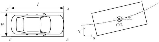
Figure 3. Rectangular vehicle model.

Assume that the size of the ego vehicle is the same as that of other traffic vehicles, and the surrounding traffic vehicles keep constant velocity in a straight line during the lane change process. According to the lane change trajectory function of Equation (1), the coordinates of the centroid of the ego vehicle at time $t$ can be calculated, and the coordinates of the vertices A, B, C, and D at time $t$ can be obtained by combining the heading angle $\phi \left(t\right)$. The calculation method is as follows:

$$\begin{array}{c}\left[\begin{array}{cccc}{x}_A\left(t\right)& x_B\left(t\right)& x_C\left(t\right)& x_D\left(t\right)\\ y_A\left(t\right)& y_B\left(t\right)& y_C\left(t\right)& y_D\left(t\right)\end{array}\right]=\left[\begin{array}{cc}\cos \phi \left(t\right)& -\sin \phi \left(t\right)\\ \sin \phi \left(t\right)& \cos \phi \left(t\right)\end{array}\right]\times \frac{1}{2}\left[\begin{array}{cccc}l& l& -l& -l\\ w& -w& -w& w\end{array}\right]\\ +\left[\begin{array}{cccc}x\left(t\right)& x\left(t\right)& x\left(t\right)& x\left(t\right)\\ y\left(t\right)& y\left(t\right)& y\left(t\right)& y\left(t\right)\end{array}\right]\end{array}$$

(5)

$$\phi \left(t\right)=\arctan \frac{dy}{dx}\left(t\right)$$

(6)

Similarly, vertex coordinates of other traffic vehicles at time $t$ can be obtained as follows:

$$\left[\begin{array}{cccc}{x}_{iA}\left(t\right)& x_{iB}\left(t\right)& x_{iC}\left(t\right)& x_{iD}\left(t\right)\\ y_{iA}\left(t\right)& y_{iB}\left(t\right)& y_{iC}\left(t\right)& y_{iD}\left(t\right)\end{array}\right]=\frac{1}{2}\left[\begin{array}{cccc}l& l& -l& -l\\ w& -w& -w& w\end{array}\right]+\left[\begin{array}{cccc}{x}_i\left(t\right)& x_i\left(t\right)& x_i\left(t\right)& x_i\left(t\right)\\ y_i\left(t\right)& y_i\left(t\right)& y_i\left(t\right)& y_i\left(t\right)\end{array}\right]$$

(7)

where $i=V_{ft},V_{fc},V_{rc}$.

This study further simplifies collision detection during lane changing by creating an axially aligned bounding box. Firstly, the ego vehicle and the surrounding traffic vehicles are projected in the coordinate axis direction. When the two coordinate axes overlap, the two vehicles are judged to have a collision, as shown in the red area in Figure 4. In other words, if the coordinates of the ego vehicle and surrounding vehicles meet Equation (8) in the lane changing process, no collision will occur, and lane changing collision will be detected every 0.5 s.

$$\{\begin{array}{l}{x}_{\min }>x_{i,\max }\\ y_{\min }>y_{i,\max }\\ x_{i,\min }>x_{\max }\\ y_{i,\max }>y_{\max }\end{array}$$

(8)

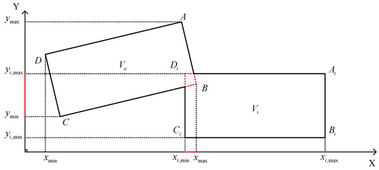
Figure 4. Schematic diagram of collision during lane changing.

When the lane changing trajectory constraint conditions of Section 2.1.1 in which the velocity of the ego vehicle is 50 km/h <= $v_e<=$ 60 km/h are added, the minimum lane changing time is 1.171 s, collision avoidance meets the algorithm of Section 2.2, and the feasible lane changing trajectory cluster is finally obtained, as shown in Figure 5. The ego vehicle is relatively safe and comfortable to drive with these trajectories.

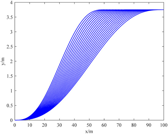
Figure 5. Feasible lane changing trajectory cluster.

2.3. NSGA-II Multi-Objective Optimization and Decision Algorithm

2.3.1. The Objective Function

In the feasible lane changing trajectory cluster, it is necessary to find an optimal lane change trajectory. In this study, the lane changing trajectory is optimized from three aspects: lane changing comfort, lane changing smoothness, and lane changing efficiency, and the influence on traffic flow to obtain the following three objective function formulas:

(1)

The weighted root mean square value of acceleration characterizes lane changing comfort:

$$WRMS={\alpha }_{1}RMS\left(\ddot{x}\left(t\right)\right)+{\alpha }_{2}RMS\left(\ddot{y}\left(t\right)\right)$$

(9)

where ${\alpha }_1={\alpha }_2=0.5$.

(2)

The maximum curvature characterizes lane changing smoothness:

$${\rho }_{\max }=Max\frac{\left|\frac{d^{2}y}{d{x}^2}\right|}{{\left[1+{\left(\frac{dy}{dx}\right)}^2\right]}^{\frac{3}{2}}}$$

(10)

(3)

Lane changing trajectory length represents lane changing efficiency and its impact on traffic flow:

$$s={\displaystyle {\int }_0^{\Delta x}\sqrt{1+{\left(\frac{dy}{dx}\right)}^2}}dx$$

(11)

where $\Delta x$ is the longitudinal displacement.

2.3.2. Multiple Objective Optimization

In this study, the optimization objective functions $WRMS$, ${\rho }_{\max }$, and $s$ cannot be minimized at the same time. Only three optimization objectives are weighed to obtain the Pareto optimal solution set, and then a further decision is made to obtain the optimal solution. In this study, the NSGA-II Algorithm [36] is used to solve nonlinear optimization problems, and the specific process is shown in Figure 6.

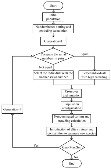
Figure 6. Optimization process of Non-Dominated Sorting Genetic Algorithm II (NSGA-II).

As the core of the NSGA-II Algorithm, it is necessary to explain non-dominant sorting in more detail. For $n$ minimization objective functions $f_i\left(x\right),i=1,2,\cdots ,n$, for any decision variables $X_a$ and $X_b$, if the following two conditions are true, then $X_b$ is dominated by $X_a$, and the constraint conditions are:

(1)

$\forall i\in 1,2,\cdots n,f_i\left(X_a\right)\le f_i\left(X_b\right)$.

(2)

$\exists i\in 1,2,\cdots n,f_i\left(X_a\right)<f_i\left(X_b\right)$.

In a group of solutions, the Pareto level of the non-dominated solution is one, which is deleted from the solution set, and the Pareto level of remaining solutions is two. By analogy, the Pareto level of all solutions in the solution set is finally obtained.

Before applying the NSGA-II Algorithm, the parameters are set as follows:

(1)

Population size: In order to obtain the global optimal solution, the population size should not be too small, but the size should also not be too large considering the time complexity. In this study, the population number is set as 100.

(2)

Crossover probability and mutation probability: Crossover probability and mutation probability were set as 0.8 and 0.2, respectively, in this study.

(3)

Maximum evolutionary algebra: Matlab simulation results showed that the evolution can be completed after 30 generations. Therefore, $MaxGen=30$.

The lane changing longitudinal displacement $\Delta x$ and lane changing duration $\Delta t$ in the scenario in Section 2.1 are decision variables, and the value range and step size satisfy Equation (12).

$$\{\begin{array}{l}80\le \Delta x\le 135\\ 4\le \Delta t\le 8\end{array}$$

(12)

where the step size of $\Delta x$ and $\Delta t$ is 0.2 m and 0.2 s, respectively.

2.3.3. Non-Dominated Sorting Method

Specific to this study, give a rank to each individual (trajectory) in the population based on non-domination, and then sort all individuals (trajectories) in descending order. If the value of at least one objective function of trajectory $p$ is better than that of trajectory $q$, and the value of other objective functions of trajectory $p$ is not worse than that of trajectory $q$, it is said that trajectory $p$ dominates trajectory $q$, and the order value of trajectory $p$ is higher than that of trajectory $q$. In the process of sorting, the trajectory with an order value of one is ranked as the first frontier, and the trajectory with an order value of two is ranked as the second frontier. After the trajectory population is sorted, the first frontier trajectory individual is completely independent of other trajectory individuals, and each frontier trajectory individual after the first frontier is dominated by the previous frontier. So far, the trajectory individuals in the trajectory population are divided into different frontiers.

The Pareto solution set is finally solved, as shown in Figure 7.

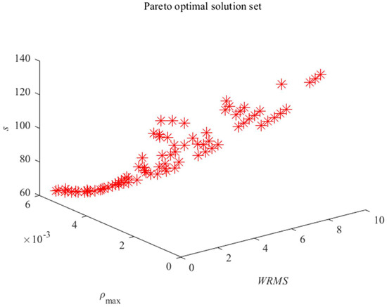
Figure 7. Pareto optimal solution set diagram.

2.3.4. Multiple Objective Decision Making

On the basis of the Pareto optimal solution set, this section takes three objective optimization functions as evaluation indicators and introduces the COWA [37,38] operator to calculate the weight of the three indicators, which can effectively weaken the impact of extreme solutions in a Pareto optimal solution set on objective weighting. Then, the TOPSIS [39] method is adopted to make decisions to obtain the solutions in the top five orders in the Pareto optimal solution set. The specific decision-making calculation process is as follows:

(1)

Take three objective optimization functions as indicators to evaluate $t$ solutions in the Pareto optimal solution set and obtain the indicator matrix $I$:

$$I={\left(i_{mn}\right)}_{t\times 3}\left(m=1,2,\cdots t;n=1,2,3\right)$$

(13)

where $i_{mn}$ is the value of the $n$th objective function of the $m$th solution.

(2)

Standardize each element of indicator matrix $I$:

$$i_{mn}^{\ast }=\frac{i_{mn}}{i_{\max ,n}}$$

(14)

where $i_{\max ,n}$ is the maximum value of the $n$th objective function.

(3)

Using the COWA operator to calculate the weight of the three objective functions ${\omega }_n$:

$${\omega }_n=\frac{{\omega }_n^{\ast }}{{\displaystyle \sum _{n=1}^3{\omega }_n^{\ast }}}$$

(15)

where ${\omega }_n^{\ast }={\displaystyle \sum _{m=1}^t{\tau }_m\cdot i_{mn}^{\ast }}$, ${\tau }_m=\frac{C_{t-1}^{m-1}}{{\displaystyle \sum _{j=0}^{t-1}{C}_{t-1}^j}}=\frac{C_{t-1}^{m-1}}{2^{t-1}}$, $C_{t-1}^{m-1}$ is the combination number of $m-1$ elements arbitrarily extracted from $t-1$ elements.

(4)

Assign weight to each element of indicator matrix $I$ to obtain the weighting matrix $K$:

$$K={\left(k_{mn}\right)}_{t\times 3}\left(m=1,2,\cdots ,t;n=1,2,3\right)$$

(16)

where $k_{mn}$ = $i_{mn}^{\ast }\cdot {\omega }_n$

(5)

Take the minimum element of the $m$th column in the weighting matrix $K$ as the optimal solution $S_n^{+}$ and the maximum element as the worst solution $S_n^{-}$, respectively:

$$S_n^{+}=\min \left(k_{1n},k_{2n},\cdots ,k_{3n}\right)$$

(17)

$$S_n^{-}=\max \left(k_{1n},k_{2n},\cdots ,k_{3n}\right)$$

(18)

(6)

Calculate the distance between elements $k_{mn}$ in the weighting matrix $K$ and $S_n^{+}$, $S_n^{-}$——$D_m^{+}$, and $D_m^{-}$, respectively:

$$D_m^{+}=\sqrt{{\displaystyle \sum _{n=1}^3{\left(k_{mn}-S_n^{+}\right)}^2}}$$

(19)

$$D_m^{-}=\sqrt{{\displaystyle \sum _{n=1}^3{\left(k_{mn}-S_n^{-}\right)}^2}}$$

(20)

(7)

Calculate the proximity index $R_m$ between the $m$th solution in the Pareto optimal solution set and the optimal level:

$$R_m=\frac{D_m^{-}}{D_m^{+}+D_m^{-}}$$

(21)

Sort the results in descending order. The solution with the largest $R_m$-value is optimal.

2.4. Optimization and Decision Result Analysis

The proposed method is implemented and tested based on MATLAB. The computer is loaded with a Windows system with AMD Ryzen5 3.0 GHz processor and 16 GB memory.

The weights of the three optimization objective functions are calculated by Equations (13)–(15) as follows: ${\omega }_1=$0.2940, ${\omega }_2=$0.2157, and ${\omega }_3=$0.4903. The top five solutions in the Pareto optimal solution set obtained through TOPSIS decision making are shown in Table 2.

Table 2. The top 5 solutions in the Pareto optimal solution set.

Order	The Decision Variables		Objective Optimization Function			${\mathit{R}}_{\mathit{m}}$
	Longitudinal Displacement/m	Time /s	$\mathit{W}\mathit{R}\mathit{M}\mathit{S}$	${\mathit{\rho }}_{\mathbf{max}}$	$\mathit{s}$ /m
1	78	5.2	0.5947	0.0035	78.1286	0.9160
2	80	5.2	0.5827	0.0034	80.1254	0.9154
3	76	5.0	0.6137	0.0037	76.1320	0.9148
4	82	5.4	0.5478	0.0032	82.1223	0.9136
5	80	5.8	0.8051	0.0034	80.1254	0.9118

Therefore, the longitudinal displacement of lane changing is finally determined to be 78 m, and the lane changing time is 5.2 s. The optimal lane changing trajectory function can be obtained by substituting the two parameters into Equation (1) and combining the state quantities at the initial and termination moments of the ego vehicle lane changing. The lane changing trajectories of the ego vehicle and other surrounding vehicles are shown in Figure 8, where $V_e$ represents the ego vehicle, $V_{fc}$ represents the vehicle in front of the current line, $V_{ft}$ represents the vehicle in front of the target line, and $V_{rt}$ represents the vehicle in rear of the target line.

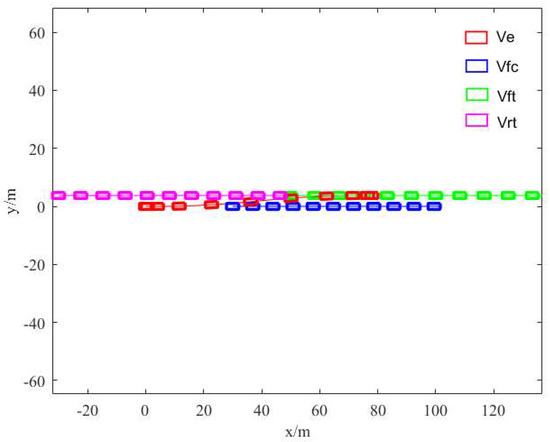
Figure 8. Lane changing trajectories of the ego vehicle and other surrounding vehicles.

In Equation (1), the lateral trajectory is a function of the longitudinal displacement $x$. The lateral velocity and acceleration can be obtained by Equation (22).

$$\{\begin{array}{l}\dot{y}\left(t\right)=\dot{y}\left(x\right)\dot{x}\left(t\right)\\ \ddot{y}\left(t\right)=\ddot{y}\left(x\right){\dot{x}}^2\left(t\right)+\dot{y}\left(x\right)\ddot{x}\left(t\right)\end{array}$$

(22)

Then, the longitudinal and lateral displacement, velocity, acceleration, yaw angle, curvature, and other information of the vehicle are obtained, and the schematic diagram of these variables with time is drawn by Matlab as follows (Figure 9).

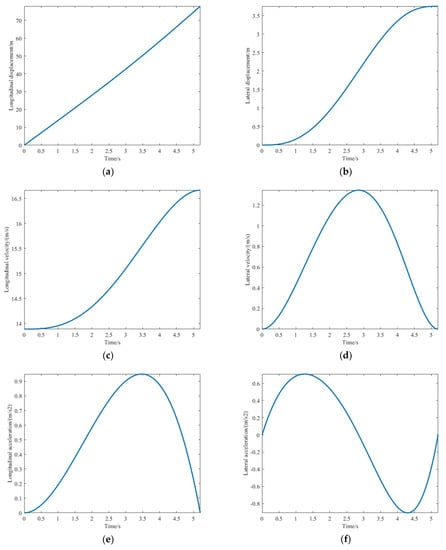
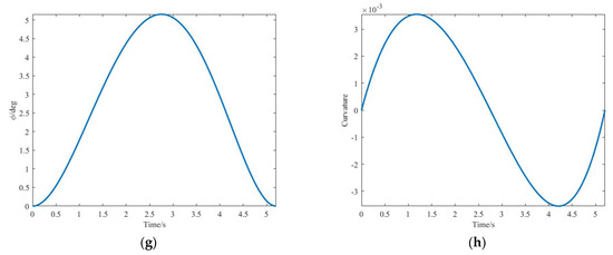
Figure 9. Driving state of the ego vehicle under optimal lane changing trajectory. (a) Longitudinal displacement curve. (b) Lateral displacement curve. (c) Longitudinal velocity curve. (d) Lateral velocity curve. (e) Longitudinal acceleration curve. (f) Lateral acceleration curve. (g) Heading angle curve. (h) Curvature curve.

It can be seen from the figure that the displacement, velocity, and curvature of the planned trajectory are smooth and continuous. The longitudinal velocity is gently accelerated from 13.89 m/s to 16.67 m/s, and the lateral velocity is gently accelerated from 0 to 1.35 m/s and then slowed down to 0. The lane changing process is relatively stable. The maximum value of longitudinal acceleration is about 0.95 m/s², the maximum value of lateral acceleration is about 0.91 m/s², and the acceleration value of the start and end of lane changing is 0. The optimal lane changing path designed in this study conforms to the constraints of lane changing trajectory and is suitable to be used as the actual lane changing reference trajectory.

The path planning method in [20] is compared with the proposed method. Similar to the lane change scenario in [20], the maximum curvature of the lane change trajectory planned in this study is 0.0221/m, which is smaller than that in [20] (0.05729/m), and the lane changing velocity and acceleration curves in [20] are not smooth. The comparison shows that the method proposed in this study can ensure a more stable and comfortable lane changing process.

3. Conclusions

An optimal lane change path planning algorithm based on NSGA-II and TOPSIS is proposed in this paper, and the vehicle lane change trajectory is generated based on a quintic polynomial. Firstly, feasible lane change trajectory clusters are obtained based on lane change constraints and an obstacle avoidance algorithm. Firstly, feasible lane change trajectory clusters are obtained based on lane change constraints and an obstacle avoidance algorithm. Then, a multi-objective optimization method for lane change trajectory based on NSGA-II is proposed, which takes into account the comfort, stability, efficiency, and impact on traffic flow. On this basis, the COWA operator is introduced to calculate the weights of three objective optimization functions. Finally, the TOPSIS Algorithm is applied to obtain the optimal lane change path. The simulation results show that the displacement, velocity, and curvature of the optimal lane change trajectory planned by the method proposed in this paper are smooth and continuous and meet the constraints of the lane change trajectory, which is suitable for the actual lane change reference trajectory.

However, there still exist some research limitations that future works will be required to be addressed. Firstly, we hope to further improve the efficiency of the algorithm, making the lane change path planning response faster. Moreover, in the process of lane changing, the prediction of the surrounding traffic vehicle trajectory will be added to make the collision detection more reasonable. In addition, the method proposed in this paper will be combined with the trajectory tracking control algorithm. The rationality of the algorithm will be verified by the vehicle dynamics software, and the vehicle yaw rate and other dynamic characteristics during lane changing will be analyzed to see if they meet the requirements.

References

- National Center for Statistics and Analysis. Overview of the 2021 Crash Investigation Sampling System; National Highway Traffic Safety Administration: Washington, DC, USA, 2022.
- Liu, Y.; Zhou, B.; Wang, X.; Li, L.; Cheng, S.; Chen, Z.; Li, G.; Zhang, L. Dynamic Lane-Changing Trajectory Planning for Autonomous Vehicles Based on Discrete Global Trajectory. IEEE Trans. Intell. Transp. Syst. 2021, 23, 8513–8527. [Google Scholar] [CrossRef]
- Singh, S. Critical Reasons for Crashes Investigated in the National Motor Vehicle Crash Causation Survey; Traffic Safety Facts Crash Stats. Report No. Dot Hs 812 506; National Highway Traffic Safety Administration: Washington, DC, USA, 2018.
- Ding, Y.; Zhuang, W.; Wang, L.; Liu, J.; Guvenc, L.; Li, Z. Safe and Optimal Lane-Change Path Planning for Automated Driving. Proc. Inst. Mech. Eng. Part D J. Automob. Eng. 2021, 235, 1070–1083. [Google Scholar] [CrossRef]
- Amer, N.H.; Zamzuri, H.; Hudha, K.; Kadir, Z.A. Modelling and Control Strategies in Path Tracking Control for Autonomous Ground Vehicles: A Review of State of the Art and Challenges. J. Intell. Robot. Syst. 2017, 86, 225–254. [Google Scholar] [CrossRef]
- Zhu, F.; Xu, X.; Ma, L.; Guo, D.; Cui, X.; Kong, Q. Autonomous driving vehicle control auto-calibration system: An industry-level, data-driven and learning-based vehicle longitudinal dynamic calibrating algorithm. In Proceedings of the 2020 IEEE Intelligent Vehicles Symposium (IV), Las Vegas, NV, USA, 19 October–13 November 2020; IEEE: New York, NY, USA, 2020; pp. 391–397. [Google Scholar]
- Geyer, J.; Kassahun, Y.; Mahmudi, M.; Ricou, X.; Durgesh, R.; Chung, A.S.; Hauswald, L.; Pham, V.H.; Mühlegg, M.; Dorn, S.; et al. A2d2: Audi Autonomous Driving Dataset; Cornell University: Ithaca, NY, USA, 2020. [Google Scholar]
- Grigorescu, S.; Trasnea, B.; Cocias, T.; Macesanu, G. A Survey of Deep Learning Techniques for Autonomous Driving. J. Field Robot. 2020, 37, 362–386. [Google Scholar] [CrossRef]
- Caesar, H.; Bankiti, V.; Lang, H.; Vora, S.; Liong, V.E.; Xu, Q.; Krishnan, A.; Pan, Y.; Baldan, G.; Beijbom, O. nuScenes: A multimodal dataset for autonomous driving. In Proceedings of the IEEE/CVF Conference on Computer Vision and Pattern Recognition (CVPR), Seattle, WA, USA, 13–19 June 2020; pp. 11621–11631. [Google Scholar]
- Huang, C.; Huang, H.; Hang, P.; Gao, H.; Wu, J.; Huang, Z.; Lv, C. Personalized Trajectory Planning and Control of Lane-Change Maneuvers for Autonomous Driving. IEEE Trans. Veh. Technol. 2021, 70, 5511–5523. [Google Scholar] [CrossRef]
- Liu, X.; Liang, J.; Fu, J. A Dynamic Trajectory Planning Method for Lane-Changing Maneuver of Connected and Automated Vehicles. Proc. Inst. Mech. Eng. Part D J. Automob. Eng. 2021, 235, 1808–1824. [Google Scholar] [CrossRef]
- Zheng, H.; Zhou, J.; Shao, Q.; Wang, Y. Investigation of a Longitudinal and Lateral Lane-Changing Motion Planning Model for Intelligent Vehicles in Dynamical Driving Environments. IEEE Access 2019, 7, 44783–44802. [Google Scholar] [CrossRef]
- Harding, J.; Powell, G.; Yoon, R.; Fikentscher, J.; Doyle, C.; Sade, D.; Lukuc, M.; Simons, J.; Wang, J. Vehicle-To-Vehicle Communications: Readiness of v2v Technology for Application; Dot Hs 812 014; National Highway Traffic Safety Administration: Washington, DC, USA, 2014.
- Kong, L.; Khan, M.K.; Wu, F.; Chen, G.; Zeng, P. Millimeter-Wave Wireless Communications for Iot-Cloud Supported Autonomous Vehicles: Overview, Design, and Challenges. IEEE Commun. Mag. 2017, 55, 62–68. [Google Scholar] [CrossRef]
- Ullah, H.; Gopalakrishnan Nair, N.; Moore, A.; Nugent, C.; Muschamp, P.; Cuevas, M. 5G Communication: An Overview of Vehicle-To-Everything, Drones, and Healthcare Use-Cases. IEEE Access 2019, 7, 37251–37268. [Google Scholar] [CrossRef]
- Liu, Y.; Wang, X.; Li, L.; Cheng, S.; Chen, Z. A Novel Lane Change Decision-Making Model of Autonomous Vehicle Based on Support Vector Machine. IEEE Access 2019, 7, 26543–26550. [Google Scholar] [CrossRef]
- Wang, W.; Qie, T.; Yang, C.; Liu, W.; Xiang, C.; Huang, K. An Intelligent Lane-Changing Behavior Prediction and Decision-Making Strategy for an Autonomous Vehicle. IEEE Trans. Ind. Electron. 2022, 69, 2927–2937. [Google Scholar] [CrossRef]
- Turkoglu, K.; Selvakumar, J. Application of Chance-Constrained and Sample-Based Path Search for High Level Behavioural Planning: A Case Study of Autonomous Highway Lane Change Scenario; Aiaa Scitech 2020 Forum; American Institute of Aeronautics and Astronautics: Orlando, FL, USA, 2020. [Google Scholar]
- Bae, I.; Kim, J.H.; Moon, J.; Kim, S. Lane change maneuver based on bezier curve providing comfort experience for autonomous vehicle users. In Proceedings of the 2019 IEEE Intelligent Transportation Systems Conference (ITSC), Auckland, New Zealand, 27–30 October 2019; IEEE: New York, NY, USA, 2019; pp. 2272–2277. [Google Scholar]
- Zeng, D.; Yu, Z.; Xiong, L.; Zhao, J.; Zhang, P.; Li, Z.; Fu, Z.; Yao, J.; Zhou, Y. A Novel robust lane change trajectory planning method for autonomous vehicle. In Proceedings of the 2019 IEEE Intelligent Vehicles Symposium (IV), Paris, France, 9–12 June 2019; IEEE: New York, NY, USA, 2019; pp. 486–493. [Google Scholar]
- Li, Z.; Liang, H.; Zhao, P.; Wang, S.; Zhu, H. Efficent lane change path planning based on quintic spline for autonomous vehicles. In Proceedings of the 2020 IEEE International Conference on Mechatronics and Automation (ICMA), Beijing, China, 13–16 October 2020; IEEE: New York, NY, USA, 2020; pp. 338–344. [Google Scholar]
- Norouzi, A.; Kazemi, R.; Abbassi, O.R. Path Planning and Re-Planning of Lane Change Manoeuvres in Dynamic Traffic Environments. Int. J. Syst. Sci. 2019, 14, 239. [Google Scholar] [CrossRef]
- Bai, H.; Shen, J.; Wei, L.; Feng, Z. Accelerated Lane-Changing Trajectory Planning of Automated Vehicles with Vehicle-To-Vehicle Collaboration. J. Adv. Transp. 2017, 2017, 1–11. [Google Scholar] [CrossRef]
- XI, C.; Shi, T.; Wu, Y.; Sun, L. Efficient motion planning for automated lane change based on imitation learning and mixed-integer optimization. In Proceedings of the 2020 IEEE 23rd International Conference on Intelligent Transportation Systems (ITSC), Rhodes, Greece, 20–23 September 2020. [Google Scholar]
- Luo, Y.; Xiang, Y.; Cao, K.; Li, K. A Dynamic Automated Lane Change Maneuver Based on Vehicle-To-Vehicle Communication. Transp. Res. Part C-Emerg. Technol. 2016, 62, 87–102. [Google Scholar] [CrossRef]
- Othman, N.A.; Reif, U.; Ramli, A.; Misro, M. Manoeuvring Speed Estimation of a Lane-Change System Using Geometric Hermite Interpolation. Ain Shams Eng. J. 2021, 12, 4015–4021. [Google Scholar] [CrossRef]
- Wang, J.; Zhang, Q.; Zhang, Z.; Yan, X. Structured Trajectory Planning of Collision-Free Lane Change Using the Vehicle-Driver Integration Data. Sci. China Technol. Sci. 2016, 59, 825–831. [Google Scholar] [CrossRef]
- Qiao, B.; Wu, X. Lane change control of autonomous vehicle with real-time rerouting function. In Proceedings of the 2019 IEEE/Asme International Conference on Advanced Intelligent Mechatronics (AIM), Hong Kong, China, 8–12 July 2019; IEEE: New York, NY, USA, 2019; pp. 1317–1322. [Google Scholar]
- Li, Z.; Jiang, J.; Chen, W.-H. Automatic lane change maneuver in dynamic environment using model predictive control method. In Proceedings of the 2020 IEEE/RSJ International Conference on Intelligent Robots and Systems (IROS), Las Vegas, NV, USA, 24 October 2020–21 January 2021; IEEE: New York, NY, USA, 2020; pp. 2384–2389. [Google Scholar]
- Sugie, N.; Okuda, H.; Suzuki, T.; Haraguchi, K.; Kang, Z. Simultaneous realization of planning and control for lane-change behavior using nonlinear model predictive control. In Proceedings of the 2018 21st International Conference on Intelligent Transportation Systems (ITSC), Maui, HI, USA, 4–7 November 2018; IEEE: New York, NY, USA, 2018; pp. 2406–2411. [Google Scholar]
- Wang, H.; Lu, B.; Li, J.; Liu, T.; Xing, Y.; Lv, C.; Cao, D.; Li, J.; Zhang, J.; Hashemi, E. Risk Assessment and Mitigation in Local Path Planning for Autonomous Vehicles With Lstm Based Predictive Model. IEEE Trans. Autom. Sci. Eng. 2021, 19, 2738–2749. [Google Scholar] [CrossRef]
- Zhou, J.; Zheng, H.; Wang, J.; Wang, Y.; Zhang, B.; Shao, Q. Multiobjective Optimization of Lane-Changing Strategy for Intelligent Vehicles in Complex Driving Environments. IEEE Trans. Veh. Technol. 2020, 69, 1291–1308. [Google Scholar] [CrossRef]
- Peng, T.; Su, L.; Zhang, R.; Guan, Z.; Zhao, H.; Qiu, Z.; Zong, C.; Xu, H. A New Safe Lane-Change Trajectory Model and Collision Avoidance Control Method for Automatic Driving Vehicles. Expert Syst. Appl. 2020, 141, 112953. [Google Scholar] [CrossRef]
- Jula, H.; Kosmatopoulos, E.B.; Ioannou, P.A. Collision Avoidance Analysis for Lane Changing and Merging. IEEE Trans. Veh. Technol. 2000, 49, 2295–2308. [Google Scholar] [CrossRef]
- You, F.; Zhang, R.; Lie, G.; Wang, H.; Wen, H.; Xu, J. Trajectory Planning and Tracking Control for Autonomous Lane Change Maneuver Based on the Cooperative Vehicle Infrastructure System. Expert Syst. Appl. 2015, 42, 5932–5946. [Google Scholar] [CrossRef]
- Deb, K.; Pratap, A.; Agarwal, S.; Meyarivan, T. A Fast and Elitist Multiobjective Genetic Algorithm: Nsga-Ii. IEEE Trans. Evol. Comput. 2002, 6, 182–197. [Google Scholar] [CrossRef]
- Jin, F.; Ni, Z.; Chen, H.; Li, Y.; Zhou, L. Multiple Attribute Group Decision Making Based on Interval-Valued Hesitant Fuzzy Information Measures. Comput. Ind. Eng. 2016, 101, 103–115. [Google Scholar] [CrossRef]
- Tang, H.-C.; Yang, S.-T. Optimizing Three-Dimensional Constrained Ordered Weighted Averaging Aggregation Problem with Bounded Variables. Mathematics 2018, 6, 172. [Google Scholar] [CrossRef]
- Behzadian, M.; Otaghsara, S.K.; Yazdani, M.; Ignatius, J. A State-of The-Art Survey of Topsis Applications. Expert Syst. Appl. 2012, 17, 39. [Google Scholar] [CrossRef]
Disclaimer/Publisher’s Note: The statements, opinions and data contained in all publications are solely those of the individual author(s) and contributor(s) and not of MDPI and/or the editor(s). MDPI and/or the editor(s) disclaim responsibility for any injury to people or property resulting from any ideas, methods, instructions or products referred to in the content. |
© 2023 by the authors. Licensee MDPI, Basel, Switzerland. This article is an open access article distributed under the terms and conditions of the Creative Commons Attribution (CC BY) license (https://creativecommons.org/licenses/by/4.0/).