Featured Application
This heatmap analysis of positional behavior in table tennis can open the way for a more detailed analysis that can have far-reaching practical impacts on both tactical training and competitive match playing.
Abstract
(1) Background: Computer-based analyses have been widely used to study aspects of various team and racket sports. However, such analyses have so far eluded table tennis, except in special competition forms, under fixed laboratory conditions or have only tracked the ball. The aim was to detect a basic, global, positional behavior, independent of the score. (2) Methods: We investigated the player position of professional male table tennis players with respect to handedness (right/left), playing system (offensive/defensive) and racket holding (shakehand/penholder) to determine the applicability of automated analysis systems. We used existing video data of competitive matches (N = 198 sets; 2006–2020) and transliterated them into an x–y coordinate system. From this, we were able to conduct a heatmap analysis for different types of players. (3) Results: The comparison between right- and left-handed players resulted in a significant difference in the positioning of the x coordinate (D = 0.5663; p = 0.001). Both groups positioned themselves on average in their own backhanded half of the table (Re: x = −0.22 m, Li: x = 0.39 m). (4) Conclusions: Our results have yielded valuable insights into the importance of analyzing positional behavior in a differentiated manner depending on handedness, playing strategy and racket holding posture.
1. Introduction
Many racket sports such as tennis, badminton and squash use automated tracking systems for player recognition. This enables the tactical exploration of player skill for training and competition and/or performance evaluation [1]. In tennis, automatic match analysis using vision-based technology already exists (e.g., [2]). Jiang et al. (2009) developed an algorithm to detect the court lines from a broadcast video and created adaptive player figures of tennis players [3]. To track tennis players within the competition and to recognize the strokes played, Bloom and Bradley (2003) proposed a three-step procedure involving player finding, player tracking and stroke recognition [4].
Many researchers have pointed out a variety of problems with automated match analyses (e.g., camera movements, pan and zoom, fast changes in the background). In badminton, Wheat and colleagues (2014) used consumer depth cameras to create a separation between the players and their environment and were able to show an accurate tracking system in an on-court environment (e.g., player positions, moving trajectories) [5]. In badminton too, there are sport-specific problems that reduce the accuracy of player tracking. For example, the net often occludes players on the far side of the court, which can only be bypassed by using multiple, synchronized cameras [6]. Brumann and Kukuk (2017) used a camera position from vertically above the court to avoid the players blocking each other while shifting their positions variably [7]. They compared the position data of players in squash generated by an automatic acquisition system with the positions of these players evaluated manually. Their findings indicated a similarity between automated and manual acquisition of 72.47%, so the comparison of manual evaluations almost coincides with the automated ones.
The aim of this study was to propose a methodological approach to analyze the table positions of players in table tennis games through an automated tracking system using certain predefined factors for assessment. In table tennis, match analyses go back to the 1970s when the coaches used manual notations to identify strengths and weaknesses or specific tactics of individual players (e.g., [8,9]; for a review, see [10]). Modern ‘manual’ analysis—partly computer-assisted, partly pen-and-paper-based—uses predefined markers to shorten analysis time and evaluation steps (e.g., [11,12,13]). Regardless, these steps are still rather time-consuming and, therefore, usually can only be used in the analysis of a few individual competitions or players. For a more global overview of the players’ movement behavior, automated systems are critical to draw valid conclusions and elucidate training implications from larger datasets. To the best of our knowledge, this study is the first automated technical approach to track the positions of table tennis players in a real game situation and to recognize tactical structures for making recommendations thereof.
The process of professionalization of table tennis has been accompanied by an increasingly detailed analysis of individual players [14]. However, so far, there have been no fully automated systems for the real-time analysis of a table tennis match. Most studies in table tennis have focused on tracking the ball. This usually involves analyzing ball trajectories and their associated tactical placements in a competitive game [15,16,17]. There are a wide variety of solely technical problems, which exist in the automated analysis of table tennis matches. Wong and Dooley (2011) summarized the problems of an automated (computer) system to track the ball and the player during a table tennis match [18]. They concluded that the biggest challenge for video analyses in table tennis is the high speed of the ball. The ball reaches speeds of up to 160 km/h and ball rotations of 151 revolutions per second [19]. Furthermore, there are several moving objects (e.g., ball, rackets, players, cameras, umpires, crowd), which also complicate data collection and analysis. The occlusion of the ball through the racket or the player is a technical problem as it prevents any continuous tracking [17]. Wong (2009) as well as Wong and Dooley (2011) demonstrated an automated system which could help umpires to make quick and precise decisions over the validity of a table tennis serve (whether the serve is correct or incorrect) [18,20]. They used a combination of spatial and temporal information from several real match video sequences to detect the ball. This system is effective for different players and perspectives and works with a complex and reasonably static movement, such as the serve. However, the serve is a static initial condition, and, in a rally, the actions are often too complex for the system to catch.
Other conditions that make automatic detection of the ball difficult, as identified by Wong and Dooley (2011), include the small size of the ball (which is often a small percent of the size of the frame) and the low contrast between the ball and the background [18]. For certain (isolated) game situations, Djokic et al. (2020) could identify the position of a (fixed) player and the (moving) ball during the serve [21]. They analyzed the starting position of the players included in their dataset, i.e., the elite European table tennis players, during their serves and they could identify the corresponding ‘most used zone’ on the opponent’s side of the table automatically. These kinds of analyses of certain game situations (focusing on the serve) can be used to make recommendations and develop courses of action for an improvement in the players. In another tournament, Chiu et al. (2010) calculated the ball placements using computer simulation for players in a wheelchair during singles matches [22]. They used high-speed video cameras (60 fps) in this observation to record images from the side of the table (at an angle of 15°, lens height of 2.9 m and horizontal distance of 10 m between the table) to locate ball placements on the table. With the help of their dataset, they were able to identify particularly successful ball placements in wheelchair table tennis and identify the ball paths that have a higher likelihood of leading to winning points. The advantage of this specific tournament was that the wheelchair players use less space in the box and have fewer stroke variations simply due to their limited mobility.
Other mathematical approaches to estimate ball placements employ artificial neural networks [23], data mining processes [24], or Markov chains [25]. These methods use a few manually recorded rallies to extrapolate and infer larger datasets via algorithms. Tamaki and Saito (2015) developed an algorithm to reconstruct the 3D trajectory of a ball with unsynchronized videos without the same timing information and these are still usable for match analysis [26]. They were able to provide the spatial features of shots (e.g., the position of the ball while it bounced, its maximum height and its direction and velocity). The greatest accuracy of the ball trajectory, however, could only be demonstrated for relatively static game situations (e.g., the serve). In a running rally, inaccuracies in ball recognition due to the aforesaid limitations still occurred.
Oku and Iida (2017) placed the focus of the analysis on ball detection during an ongoing rally [27]. They demonstrated, with the help of a high-speed vision system, that they could track a table tennis ball accurately during a rally. This study had some extremely advanced laboratory settings and, therefore, technological requirements such as the auto pan-tilt technology to shoot high-resolution images of a ball with a high sampling rate, which made it possible to calculate the spin of a ball. Yuza et al. (1992) analyzed factors such as ‘use of space’ regarding the table position to create a heatmap for analysis [28]. In this context, a heatmap represented a two-dimensional diagram for visualizing positional data based on a probability function. The authors divided players into three categories based on handedness, playing strategy and racket holding. They manually annotated the x–y coordinates of players for each frame of the videos. Because this approach needed a considerable amount of time, only four professional table tennis players could be analyzed. Among the many observations, one which was notable was that the defending players put more distance between themselves and the table in comparison to offensive players (in the form of heatmaps calculated by the x–y position). In addition, defending players tended to stand more on their own backhand side to be able to play more with their forehand side.
This first approach to capture the position of players in the box during a real table tennis match in the form of heatmaps has so far not been pursued further. The study by Yuza et al. (1992) is limited by the small sample size of only four players and an outdated rule system (e.g., the set length of up to 21 points back then, which has been changed to up to 11 points now) which makes its application to analyses in today’s competitions difficult [28].
In summary, there are plenty of technical problems owing to the high speed of the moving objects during the game (e.g., the ball, the rackets, the players), the occlusion (in particular, during a serve) and the small size of the ball [18]. The study by Wong and Dooley (2011) explored the idea that in table tennis, the ball position is highly connected to the position of the players [18]. The automatic recording of table tennis players’ position in relation to the table could be much easier than tracking the ball; so, we expect precise data when we can extract them from existing video sequences of players. Sports scientists have pointed out the disadvantages of analyzing individual strokes (e.g., placements, spin variations, durations, tempos, etc.) without referencing the actions of the opponent [29]. It is important to compare players’ positions in relation to each other, because a second substantive issue in match analyses—intrinsic to all sports—is the interaction between the opponents. Moreover, every single game (or set) differs from the others, even with the same players playing against each other [30].
In the present study, the same categories (handedness, playing system and racket holding) as in the study by Yuza et al. (1992) were used as fixed factors to evaluate the following hypotheses [28]:
- It is assumed that the x positions of the left-handers and the right-handers differ, in a way that the left-handers stay more on the right side of the table and the right-handers stay more on the left side. Players are assumed to prefer this positioning, so that they can stand more on their own backhand side and play more with their forehand.
- Defending players travel more distance in the y direction than offensive players and are also positioned farther back (in the y direction) in the mean. This greater mileage should be reflected in the space/area and, where appropriate, in the x direction.
- For the racket holding (penholder vs. shakehand), the predictions are open-ended [31]. In general, for the shakehand grip, the index finger is placed on the lower part of the backhand grip and the thumb is rested on the lower part of the forehand grip of the racket. The other three fingers enclose the wood grip. For the penholder grip, both the thumb and index finger are normally placed on the forehand rubber, while the other three fingers rest on the backhand rubber. It is unclear whether a penholder racket hold generally requires less movement in the x and/or y direction because penholder players do not have to go around their changeover point (between backhand and forehand). This also holds for footwork required due to the greater reach of the shakehand grip as this too is difficult to assess in advance.
2. Materials and Methods
The video material acquired for this study, the visual recognition procedure, the producing of the heatmaps and the data analysis are described below. Publicly available videos in TV broadcast (N = 62) were shortlisted for data collection by two table tennis experts. Official competitive matches of male table tennis players of the top 100 of the ITTF (International Table Tennis Federation) world ranking were screened (types of tournaments: World Table Tennis Championships, ITTF World Tour, (Youth) Olympic Games, T2 Diamond, European Championships, ETTU—Europe Top 16, ETTU Champions League, Japan Open, Swedish Open, Czech Open, Hong Kong Open, German Open, Chinese Super League, T2 Asia-Pacific League, French League, Polish League, German League, Olympic Qualification, Marvellous 12, Düsseldorf Masters). The matches were played in best-of-five and best-of-seven modes. Our automatic extraction pipeline provided sufficient detections and dense data for 45 of the shortlisted videos due to a beneficial camera perspective (N = 198 sets). The remaining videos were rejected due to unreliable person or table detections. These videos were of high-level and championship games, each consisting of an entire match and lasting around 60 min. For each video, the focus was on one player. The analyzed matches were played from 2006 to 2020. Following Yuza et al. (1992), the players were categorized by table tennis experts according to handedness, playing strategy and racket holding [28]. The dominant hand of the players was established according to which hand was used to hold the racket [32]. The classification of the playing system was determined by two scientists who independently identified whether the player was closer to the table and played more offensive strokes (e.g., topspin: players normally tilt the paddle forward and brush it over the ball from a low to a high position in order to give the ball a forward rotation [33]) or further away from the table and played more defensive strokes (e.g., backhand chop: this is normally used by defensive players to impart backspin on the ball which makes it harder to attack. It is mostly played against a topspin stroke). Additionally, the racket position was determined for the players with whom the analyzed match had been played. Out of the 45 videos, 31 players were right-handed and 14 players were left-handed; 32 players were attack/offensive players and 13 had a more defending playing style; and 25 had the shakehand grip while holding the paddle and 20 had the racket/paddle in a penholder grip. The videos were edited and recorded in the manner of TV broadcasts, with cuts, jumps and replays. Therefore, the parts of the video that contained the actual game had to be extracted first. After data collection, the methodology was developed using one video and then applied to all of the other videos.
2.1. Procedure
Using a combination of existing deep learning solutions and low-level computer vision algorithms, we developed the following set of procedures:
- The recorded games contained different camera perspectives as well as different sequences of the game; there were not only played rallies, but also replays, set breaks and breaks between rallies. To detect only the positions of the players in the played rallies, the first step was to identify the table. For this purpose, we first extracted a set of straight lines from each frame using a Hough transform. Due to the typical camera position looking down onto the table, orthogonally to the net, the table induced a distinct set of lines. The absence of this line configuration indicated that the frame did not contain an active rally and the frame was not processed further ([34] for image processing steps) (Figure 1).
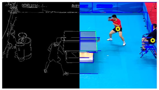 Figure 1. The transformation to edges for the Hough transform on the left side and detection of player and table position on the right side.
 - Next, the table was detected in each of the remaining frames. The lines computed in the previous step were used again to find the potential pairs of lines that could indicate the table. In Figure 1, all of the horizontal and vertical lines are specified. Green lines were the likely options for the table, whereas the blue lines were ignored. For each pair of potential lines, we finally computed whether they surrounded an area that was mainly uniform in color (e.g., green/blue as a table tennis table).
- From all valid frames, the system detected all of the people using the publicly available state-of-the-art library Detectron2, developed by Facebook Research [35]. As can be seen in Figure 1, the players, as well as the referee (or many viewers in other videos) around them, were detected (yellow circles). Simple heuristics and tracking were applied to select just the two players out of all of the detected people.
- Using the position of the table in each frame, the 2D image plane position of the players could be transformed into a 2D top view plane. We created this by projecting the 2D hip position in the image onto the detected 3D table plane, with the assumption being that players’ hips were roughly at table height. To define the positions of the players, a coordinate system was established which was relative to the table. Here, the zero point represented the exact center of the table tennis table. Since the camera was in constant motion in these videos, tracking the position of the table was crucial.
- The entire video was then split into segments, i.e., single rallies that were used to create heatmaps, such as in the example below (Figure 2). The four frames represented a rally that was around five seconds long and resulted in the player positions depicted on the right:
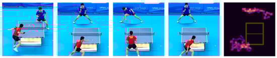 Figure 2. Four frames and their resultant player positions (https://www.youtube.com/watch?v=yRI2Y6ytdPI) (accessed on 7 June 2022).
 - To create the heatmap in Figure 2, the sequence of positions of each segment was converted into a probability map. For this purpose, we created an empty occurrence map of size 3.5 × 4 m. Each of the athletes’ (x, y) positions then incremented the count of occurrences around an area of 4.5 cm2 around (x, y) by 1. The occurrence map was then normalized by dividing it by the overall sum of all the counts in the map, resulting in the probability map.
- To combine the heatmaps from multiple rallies, time stamps were manually collected for the sets of each of the games. A set started when the ball was thrown up during the first serve and ended when the ball was terminated by losing or winning the last point of the set (e.g., bouncing on the floor, landing in the net). Variations in annotating the exact start and end frame of each set could be neglected to the millisecond because each heatmap consisted of positions over an average of 48 min per player. Each game of over 100 segments per set (interrupted by breaks, replays, viewpoint variations) was thus combined into the game sets for each player (5 sets for 1 player each). These heatmaps could be used to compare players with different playing styles. As dependent variables, we established the mean value of the x and y coordinates of a player per set, as well as the area in which the players moved. Therefore, values on the x coordinate meant positions sideways to the short side of the table. Values on the y coordinate were orthogonal to the table and indicated back and forth movements. These variables were calculated only for sets that contained at least 50 valid data points. This led to the initially mentioned filtering from 62 to 45 games.
2.2. Heatmaps
To compare the positions of the players to the table from different videos, a coordinate system was placed over the table. The zero point represented the center of the table. Up to several thousand positions were recorded per set. This resulted in a mean value for each set for both the x and the y coordinate.
For each player, we created an individual location heatmap of all of their positions during the game; each occupied an x–y position with a 4.5 cm2 area around that point. This resulted in an occurrence count over all possible locations. Normalizing this occurrence map, such that the sum over all locations equaled 1, created a probability density function of the location for each specific player. We combined the player-specific heatmaps (=probability maps) into six heatmaps for each expression (cf. Figure 3). Each expression pair (right/left, offensive/defensive, shakehand/penholder) contained information from all 45 videos (e.g., 31 videos right-handed, 14 videos left-handed). To avoid over-representation of a single expression, as well as their effects on other expressions, we performed the following normalization steps. With three attributes (handedness, playing system and racket holding) and two expressions each (right/left, offensive/defensive, shakehand/penholder), there were a total of eight possible player–type combinations. We assumed that most penholder players were right-handed. If we weighted each player equally, the heatmap for penholders would consist of mainly right-handed players and show the same effects as the right-handed heatmap. Instead, we first collected and normalized heatmaps for the eight player–type combinations and then combined these again to arrive at the six per-expression heatmaps shown in Figure 3.
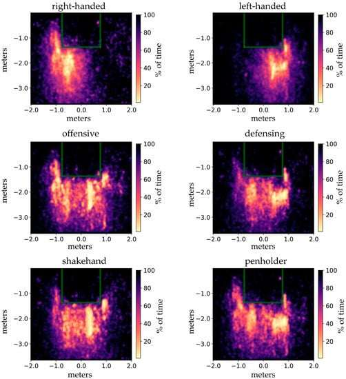
Figure 3.
Heatmap comparison for the player types differentiated for right- vs. left-handed players, offensive vs. defensive players and shakehand vs. penholder grip players. For example, a purple color (purple = 60%) indicates that the player had been in the area (purple or lighter) 60% of the time. The lighter the color (light yellow), the more often the players had been in that area.
2.3. Data Analysis
Each heatmap could be interpreted as a two-dimensional probability function, which mapped an (x, y) pair to the likelihood that a player with this expression was positioned here during a match.
We compared these 2D distributions using a variant of the Kolmogorov–Smirnov test adapted to higher dimensions, as previously used in astronomy and climate research [36,37]. Additionally, we projected the probability map to just x or y portions, respectively, and performed a conventional KS analysis (cf. Figure 4).
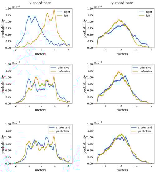
Figure 4.
The probability rate of player positions on the x and y coordinates differentiated by right-handed vs. left-handed, offensive vs. defensive and shakehand vs. penholder grip players. Kolmogorov–Smirnov test analysis for the projected x and y distributions.
Using the interpretation of each heatmap as a probability distribution, we could determine confidence intervals for the locations, i.e., the portion of the area around the table that the players spent 95% of the overall playtime in. The confidence interval was set to 95%. The displayed values were averages of overall position data.
A heatmap was created for each player expression (cf. Figure 3). The heatmap represented the density function of the different positions in the table tennis match. In each heatmap, the table tennis half was marked with a green line. The coordinate system could also be seen here. The zero point (0, 0) was exactly in the middle of the table, so a value of y = 0 m meant at the height of the net. Because the total length of a table tennis table is 2.74m, and thus the baseline of the table has a value of y = −1.37m on the y-coordinate, a value of y = −1.90m meant that a player positioned himself 53cm from the baseline. The center line of the table represented the zero point on the x coordinate. If an x value was positive, it meant that the player was positioned to the right of the center line, and if the x value was negative, it meant that the player was positioned to the left of the center line. The colors used in the heatmap represented the frequency of a position and were labeled by percentiles. For example, a color in the middle of the spectrum, purple = 60%, meant that the players spent 60% of the overall time at a location that was purple or brighter. The lighter the color (light yellow), the more often that players were in that area.
To determine the significant differences, the two-dimensional Kolmogorov–Smirnov test was calculated and implemented in Python programming language syntactically equivalent to the nature paper by Chiang et al. (2021) [36]. Significant differences in 2D distributions were found for the right/left pair (D = 0.5712, p = 0.005). The analyses for the projected x and y distributions of the player types are shown in Figure 4. Comparisons were shown between the expressions of the three attributes (right/left, offensive/defensive, shakehand/penholder). Whereas the heatmaps in Figure 3 display the probability as the color at a certain 2D location, these plots showed the x (left) and y (right) coordinates on the abscissa and the probability that a player was at this point on the ordinate.
The 1-dimensional KS test yielded significant differences for the x coordinate of the right/left (D = 0.5663, p < 0.001).
3. Results
3.1. Handedness (Right- vs. Left-Handed)
The size of the area of right-handed players was larger than that of left-handed players (right-handers’ area: 8.66 m2; left-handers’ area: 7.08 m2). For right-handers, the area was distributed more to the left side of the table, i.e., in their own backhand table half (Figure 3 and Figure 4). The other way around, the heatmap for left-handed players showed that they were positioned more in the right half of the table, i.e., also in their own backhand half (Figure 3 and Figure 4). Right-handed players were positioned in the mean value on the x coordinate of x = −0.22 m from the center line of the table to the left (their backhand side). The left-handed players had a distance of x = 0.39 m (mean values on the x coordinate) from the center line of the table to the right (own backhand side). There was a significant difference between right-handed and left-handed players in terms of positioning on the x coordinate (p = 0.005, two-dimensional Kolmogorov–Smirnov test). The mean values on the y coordinate were similar for both player types (right-handed/left-handed), so both player types moved back and forth with the similar distance to the table (right-handed: y = 2.07 m; left-handed: y = 2.25 m).
3.2. Playing Style (Offensive vs. Defensive)
The area of offensive players was larger than that of defensive players, so offensive players took up more area/space (offensive: 9.27 m2; defensive: 7.64 m2) (Figure 3). Offensive players were, on average, oriented further to the right on the x coordinate or from the center line of the table (offensive: x = 0.08 m) and defensive players, on average, oriented further to the left on the x coordinate or from the center line of the table (defensive: x = −0.03 m). There was no tendency to see whether offensive or defensive players stood further away from the table (y coordinate). Both types of players were about a similar distance from the table (offensive: y = 2.14 m; defensive: y = 2.17 m).
3.3. Racket Holding (Shakehand vs. Penholder Grip)
The area for penholder players had a higher mean value than for shakehand players (penholder: 8.79 m2; shakehand: 8.41 m2) (Figure 3). It meant that penholder players used more area/space. However, shakehand players were oriented more to the right (x coordinate: x = 0.08 m) than penholder players (x coordinate: x = −0.02 m). There was no difference between shakehand and penholder players in forward and backward positions to the table (y coordinate for both racket holdings: y = 2.15 m).
4. Discussion
Finally, we presented a method for the automatic detection of table tennis players’ positions. The parameters used to classify the players (handedness, playing style and racket holding) were chosen based on the study by Yuza et al. (1992) [28]. The primary objective was to show the feasibility of an automated way using software to distinguish handedness for the same three categories of players. There is, of course, still a need for optimization in the selection of the variables recorded.
Overall, it could be indicated that the left-handed and the right-handed players differed significantly with respect to their position data. Therefore, it can be assumed that table tennis players play not only backhand, but also with the often strong forehand side from the backhand half of the table to go around. As the stroke techniques were not analyzed in the current study, they should be investigated in follow-up studies. Due to the more frequent positioning in the backhand half of the table, balls with a side cut, for example, can be played in such a way that they are bounced in the direction of the backhand half of the table on the changing point of the opponent or bounced out sideways in the direction of the forehand half of the table. Through this, the distance between the player and ball is removed even further after bouncing. Our data suggest that offensive players are slightly more often positioned on the right half of the table. From this, it could be deduced that with many right-handed players, the game is predominantly played over the forehand half of the table. Often in offensive play, forehand topspin is played against forehand topspin. On the other hand, defensive players are more often played on their own backhand side, so that they can play the ball back with undercut defense [38,39]. Contrary to the assumption that defensive players take up more space, the results showed that defensive players position themselves in a smaller area. Reasons for this could be that defensive players tend to position themselves more on the backhand side and are played there more often [40]. Penholder players have a shorter reach purely through the technical change in the posture of the handle. This is also reflected in the results that these types of players use more area with the penholder racket holding position and thus position themselves more in this area. The shorter reaching distance of the penholder players can be used by placing the balls on the outermost sides of the table. With an appropriate side cut, the ball could be played further into the outer sides after bouncing on the table.
Regarding specific games in a match, the playing behavior can change significantly within a single set [10]. This can be a consequence of the tactical decisions made by a player, or it can happen due to certain psychological conditions. This leads to the inference that tactical measurements in team and racket sports tend to show a wide range of intra-individual fluctuations. In contrast, the types of sports that do not involve direct contact with the opponent tend to place much less weight on the tactical considerations and, thus, bring about a framework and examination conditions which are more stable [41,42]. Therefore, the process of identifying consistent behavioral traits across different matches has proven to be difficult [43]. In addition, it is important to be as variable as possible in the match, so that the opponent can hardly predict with which speed, rotation, flight altitude and positioning the ball will be played.
The position analysis always includes a total rally. Therefore, the analysis starts with the first touch of the ball, i.e., the serve. The serve is almost always executed at the corner point of the backhand half (for right-handers at the left corner of the table). This start situation can distort the position data because this position appears relatively very often (every other rally). It could be the same with the backstroke. The starting position is often the middle or the position in the own backhand table half. In further studies, the position analysis could start only with the third touch of the ball (without server and backstroke) to check if the positions during the serve or in the starting position change the general view of the positions.
Automatic position/placement detection of the ball via image recognition could lead to a breakthrough in game analyses in table tennis, just like in other games such as tennis. Consequently, match analysis could have an enormous quantity of data that are automatically collected and can be used to identify strengths and weaknesses of an opponent, to make (position-specific) self-tactical analyses or to draw conclusions for daily training (e.g., footwork; [11]).
A major shortcoming of this study is that the capturing of each player’s movement data was independent of the type of player on the opposite side. It is obvious that the players’ position and move are generally adapted to their opponent [12]. Of course, a left-handed player will play differently when facing a left-handed player resulting from a change in positioning and a defensive player will play differently against another defensive player [44]. We also did not consider the relationship between certain playing positions. However, this step was deliberately omitted in the context of this first, more methodologically oriented study, because the initial aim was to detect a basic, global, positional behavior, independent of the score. Again, it is not easy to clearly define success and failure during a table tennis match. In some cases, a player can be in the perfect position to the ball, the table and the opponent and yet fail due to a technical error or bad luck (e.g., a net roller or edge ball). Similarly, for such an accurate comparison, it would have to be ensured that the players are playing at a uniform level and the points won are due to their strategy and positioning alone and not external factors [45,46]. Both of these requirements are quite difficult to fulfil while post hoc analyzing real match situations. Although there are no significant differences, there seems to be a minor difference in the heatmaps of attacking and defending players in the left–right direction. This is due to the style of play, but not to the uneven distribution of player types. In order to counteract a dissimilar number of player types (e.g., more right-handed than left-handed defenders), the data were previously normalized and weighted. However, as already discussed, the constellation of player types in a match was not considered. Thus, there was no examination of the interaction between the two players. To find out the player positions, the hip was used as a marker to find out the table height. The players were not only of different heights and stood at different heights at the table, but also had different arm lengths with a resulting different reach. The hip marker is therefore not an exact measurement and there is an estimation error. Nevertheless, in the first methodological approach, the hip is an easily identifiable marker given in each video. It should be noted that the cameras never record the matches in exactly the same position and must therefore be recalibrated for each video.
5. Conclusions
In summary, there is an urgent need to develop largely automated analysis software in table tennis; with the help of which, matches can be analyzed in real-time in a timely, efficient and economical manner for the coaches and the players [14]. To be able to make comprehensive conclusions and recommendations, the tracking of the ball and the game situation should be included in further studies. For this purpose, the positional behavior in connection with winning points should be differentiated by handedness, playing strategy and racket holding. In addition, the position of the players in relation to each other should be compared, because another essential point in game analysis—innate to all sports—is the interaction between opposing and team players [10]. Therefore, rallies of male and female professional table tennis players in different high-class tournaments should be analyzed. The focus should be on winning and losing points. It should be investigated whether a pattern can be identified for the winning points (e.g., based on footwork, stroke technique, positioning, tempo, rotation, flight altitude and specific combinations of player types). Analysis software that can collect and process data as automatically as possible should be used.
This study can pave the way for a much more detailed analysis, which could have far-reaching practical implications for an overall improvement in the quality of the game.
Author Contributions
Conceptualization, F.H., T.B., T.K.-S., F.S. and S.K.; methodology, F.H., T.B., T.K.-S., F.S. and S.K.; software, T.B. and F.S.; validation, F.H., T.B., T.K.-S. and F.S.; formal analysis, F.H., T.B., T.K.-S. and F.S.; investigation, F.H., T.B. and T.K.-S.; resources, T.B.; data curation, F.H., T.B. and T.K.-S.; writing—original draft preparation, F.H., T.B. and T.K.-S.; writing—review and editing, F.H., T.B., T.K.-S., F.S. and S.K.; visualization, F.H. and S.K.; supervision, T.K.-S. and S.K.; project administration, S.K. All authors have read and agreed to the published version of the manuscript.
Funding
This research received no external funding.
Institutional Review Board Statement
Not applicable.
Informed Consent Statement
Not applicable.
Data Availability Statement
Publicly available videos of table tennis matches in official competitions were used to analyze the data. For this purpose, we used common video platforms (e.g., youtube.com) (accessed on 25 February 2021).
Conflicts of Interest
The authors declare no conflict of interest.
References
- Chow, J.Y.; Tan, C.W.K.; Lee, M.C.Y.; Button, C. Possibilities and implications of using a motion-tracking system in physical education. Eur. Phys. Educ. Rev. 2014, 20, 444–464. [Google Scholar] [CrossRef]
- Renò, V.; Mosca, N.; Nitti, M.; D’Orazio, T.; Guaragnella, C.; Campagnoli, D.; Prati, A.; Stella, E. A technology platform for automatic high-level tennis game analysis. Comput. Vis. Image Underst. 2017, 159, 164–175. [Google Scholar] [CrossRef]
- Jiang, Y.-C.; Lai, K.-T.; Hsieh, C.-H.; Lai, M.-F. Player Detection and Tracking in Broadcast Tennis Video. In Advances in Image and Video Technology; Wada, T., Huang, F., Lin, S., Eds.; Springer: Berlin/Heidelberg, Germany, 2009; pp. 759–770. ISBN 978-3-540-92956-7. [Google Scholar]
- Bloom, T.; Bradley, A.P. Player tracking and stroke recognition in tennis video. APRS Workshop on Digital Image Computing (WDIC’03); The University of Queensland: Brisbane, Australia, 2003; pp. 93–97. [Google Scholar]
- Wheat, J.; Lane, B.D.; Choppin, S. The accuracy of badminton player tracking using a depth camera. Depth Biomech. 2014, 3, 1–21. [Google Scholar]
- Kamiyama, T.; Kameda, Y.; Ohta, Y.; Kitahara, I. [Paper] Improvement of Badminton-Player Tracking Applying Image Pixel Compensation. MTA 2017, 5, 36–41. [Google Scholar] [CrossRef]
- Brumann, C.; Kukuk, M. Towards a better understanding of the overall health impact of the game of squash: Automatic and high-resolution motion analysis from a single camera view. Curr. Dir. Biomed. Eng. 2017, 3, 819–823. [Google Scholar] [CrossRef]
- Czwalina, C. Systematische Spielerbeobachtung in den Sportspielen [Systematic Observation of Players in Team and Racket Sport]: Zur Beobachtung Sportspielspezifischer Motorischer Qualifikationen in Basketball, Hallenhandball, Fußball und Volleyball Sowie Tennis und Tischtennis [The Observation of Team and Racket Sport Specific Motor Qualifications in Basketball, Indoor Handball, Soccer and Volleyball, As Well As Tennis and Table Tennis]; Hofmann: Schorndorf, Germany, 1976. [Google Scholar]
- Hughes, M. (Ed.) Notational Analysis of Sport: Systems for Better Coaching and Performance in Sport, 2nd ed.; Routledge: London, UK, 2004; ISBN 9780415290050. [Google Scholar]
- Straub, G.; Klein-Soetebier, T. Analytic and descriptive approaches to systematic match analysis in table tennis. Ger. J. Exerc. Sport. Res. 2017, 47, 95–102. [Google Scholar] [CrossRef]
- Malagoli Lanzoni, I.; Di Michele, R.; Merni, F. A notational analysis of shot characteristics in top-level table tennis players. Eur. J. Sport. Sci. 2014, 14, 309–317. [Google Scholar] [CrossRef]
- Muster, M. Zur Bedeutung des „situativen Trainings“ im Hochleistungstischtennis–Empirische Untersuchung zur Identifikation von „Spielsituationen“. [The Significance of „Situational Training“ in High-Performance Table Tennis–An Empirical Study for the Identification of “Game-Play Situations”]; Shaker: Aachen, Germany, 1999. [Google Scholar]
- Wu, X.-Z.; Escobar-Vargas, J. Notational analysis for competition in table tennis (part I): Based format analysis. In Proceedings of the 10th International Table Tennis Sports Science Congress; Springer: Berlin/Heidelberg, Germany, 2007; pp. 104–108. [Google Scholar]
- Fuchs, M.; Liu, R.; Malagoli Lanzoni, I.; Munivrana, G.; Straub, G.; Tamaki, S.; Yoshida, K.; Zhang, H.; Lames, M. Table tennis match analysis: A review. J. Sport. Sci. 2018, 36, 2653–2662. [Google Scholar] [CrossRef] [PubMed]
- 2006 IMACS Multiconference on Computational Engineering in Systems Applications (CESA’2006): Beijing, P.R. China, October 4–6 2006; International Association for Mathematics and Computers in Simulation; IEEE Systems, Man, and Cybernetics Society; IEEE Operations Center: Piscataway, NJ, USA, 2006; ISBN 7-302-13922-9.
- Hutchison, D.; Kanade, T.; Kittler, J.; Kleinberg, J.M.; Mattern, F.; Mitchell, J.C.; Naor, M.; Nierstrasz, O.; Pandu Rangan, C.; Steffen, B.; et al. (Eds.) Pattern Recognition and Machine Intelligence; Springer: Berlin/Heidelberg, Germany, 2005; ISBN 978-3-540-30506-4. [Google Scholar]
- Voeikov, R.; Falaleev, N.; Baikulov, R. TTNet: Real-Time Temporal and Spatial Video Analysis of Table Tennis. 2020. Available online: http://arxiv.org/pdf/2004.09927v1 (accessed on 13 June 2022).
- Wong, K. Tracking Table Tennis Balls in Real Match Scenes for Umpiring Applications. BJMCS 2011, 1, 228–241. [Google Scholar] [CrossRef] [PubMed]
- Qun, W.H.; Zhifeng, Q.; Shaofa, X.; Enting, X. Experimental research in table tennis spin. Int. J. Table Tennis Sci. 1992, 1, 73–78. [Google Scholar]
- Wong, K.C.P. Identifying table tennis balls from real match scenes using image processing and artificial intelligence techniques. Int. J. Simul. Syst. Sci. Technol. 2009, 10, 6–14. [Google Scholar]
- Djokic, Z.; Malagoli Lanzoni, I.; Katsikadelis, M.; Straub, G. Serve analyses of elite European table tennis matches. Int. J. Racket Sport. Sci. 2020, 2, 1–8. [Google Scholar] [CrossRef]
- Chiu, C.; Hung, C.; Ho, Y.; Li, T. Prediction of Ball Placement Using Computer Simulation for Wheelchair Players in Table Tennis Singles. Int. J. Sport Exerc. Sci. 2010, 2, 1–6. [Google Scholar]
- Wang, J.; Yu, L. Use the combination of the decision tree and the artificial neural networks to predict the outcome of table tennis matches. Inst. Electr. Electron. Eng. 2010, 4, 1929–1933. [Google Scholar]
- Zhang, H.; Yu, L.; Hu, J. Computer-aided game analysis of net sports in preparation of Chinese teams for Beijing Olympics. Int. J. Comput. Sci. Sport 2010, 9, 53–69. [Google Scholar]
- Pfeiffer, M.; Zhang, H.; Hohmann, A. A Markov Chain Model of Elite Table Tennis Competition. Int. J. Sport. Sci. Coach. 2010, 5, 205–222. [Google Scholar] [CrossRef]
- Tamaki, S.; Saito, H. Reconstructing the 3D trajectory of a ball with unsynchronized cameras. Int. J. Comput. Sci. Sport. 2015, 14, 3. [Google Scholar]
- Oku, H.; Iida, K. Automatic omni-directional, high-speed, pan-tilt platform. 2017. Available online: https://spie.org/news/6748-automatic-omni-directional-high-speed-pan-tilt-platform (accessed on 17 March 2021).
- Yuza, N.; Sasaoka, K.; Nishioka, N.; Matsui, Y.; Yamanaka, N.; Ogimura, I.; Takashima, N.; Miyashita, M. Game Analysis of Table Tennis in Top Japanese Players of Different Playing Styles. Int. J. Table Tennis Sci. 1992, 1, 79–89. [Google Scholar]
- Hughes, M.D.; Bartlett, R.M. The use of performance indicators in performance analysis. J. Sport. Sci. 2002, 20, 739–754. [Google Scholar] [CrossRef]
- Lames, M.; McGarry, T. On the search for reliable performance indicators in game sports. Int. J. Perform. Anal. Sport. 2007, 7, 62–79. [Google Scholar] [CrossRef]
- Aiyegbusi, A.; Oduntan, M. The relationship between grip styles and musculoskeletal injuries in table tennis players in Lagos, Nigeria: A cross-sectional study. J. Clin. Sci. 2020, 17, 52. [Google Scholar] [CrossRef]
- Peters, D.; O’Donoghue, P. (Eds.) Distribution of Stroke and Footwork Types in Top-Level Men’s and Women’s Table Tennis. Routledge: New York, NY, USA, 2013; ISBN 9780203080443. [Google Scholar]
- Safari, I.; Suherman, A.; Ali, M. The Effect of Exercise Method and Hand-Eye Coordination Towards the Accuracy of Forehand Topspin in Table Tennis. IOP Conf. Ser. Mater. Sci. Eng. 2017, 180, 12207. [Google Scholar] [CrossRef]
- Forsyth, D.A.; Ponce, J. Computer Vision: A Modern Approach, 2nd ed.; Pearson: London, UK, 2012. [Google Scholar]
- Wu, Y.; Kirillov, A.; Massa, F.; Lo, W.-Y.; Girshick, R. Detectron2. Available online: https://github.com/facebookresearch/detectron2 (accessed on 1 June 2021).
- Chiang, F.; Mazdiyasni, O.; AghaKouchak, A. Evidence of anthropogenic impacts on global drought frequency, duration, and intensity. Nat. Commun. 2021, 12, 763. [Google Scholar] [CrossRef] [PubMed]
- Peacock, J.A. Two-dimensional goodness-of-fit testing in astronomy. Mon. Not. R. Astron. Soc. 1983, 202, 615–627. [Google Scholar] [CrossRef]
- Martin, C.; Favier-Ambrosini, B.; Mousset, K.; Brault, S.; Zouhal, H.; Prioux, J. Influence of playing style on the physiological responses of offensive players in table tennis. J. Sport. Med. Phys. Fit. 2015, 55, 1517–1523. [Google Scholar]
- Straub, G. The spreading and playing ability of defensive players in competitive table tennis. Int. J. Table Tennis Sci. 2013, 8, 179–183. [Google Scholar]
- Geske, K.M.; Mueller, J. Table Tennis Tactics: Your Path to Success; Meyer & Meyer: Aachen, Germany, 2009. [Google Scholar]
- Lames, M. Methodologische Probleme der messtheoretischen Leistungsdiagnose in den Sportspielen und ein modelltheoretischer Lösungsvorschlag [Methodological problems of the measurement-based performance diagnosis and a model-theoretical proposal for solution]. Mot. Aktuell 1989, 34, 156–164. [Google Scholar]
- Lames, M. Systematische Spielbeobachtung [Systematic Game Analysis]; Philippka: Münster, Germany, 1994. [Google Scholar]
- McGarry, T.; Franks, I.M. A stochastic approach to predicting competition squash match-play. J. Sport. Sci. 1994, 12, 573–584. [Google Scholar] [CrossRef]
- Malagoli Lanzoni, I. Do left-handed players have a strategic advantage in table tennis? Int. J. Racket Sport. Sci. 2019, 1, 61–69. [Google Scholar] [CrossRef]
- Djokic, Z. Structure of competitors’ activities of top table tennis players. Int. J. Table Tennis Sci. 2002, 5, 74–90. [Google Scholar]
- International Table Tennis Federation (Ed.) Differences in Tactics in Game of Top Players and Other Factors of Success in Top Table Tennis. In Proceedings of the 9th ITTF Sports Science; ITTF: Lausanne, Switzerland, 2006. [Google Scholar]
Disclaimer/Publisher’s Note: The statements, opinions and data contained in all publications are solely those of the individual author(s) and contributor(s) and not of MDPI and/or the editor(s). MDPI and/or the editor(s) disclaim responsibility for any injury to people or property resulting from any ideas, methods, instructions or products referred to in the content. |
© 2023 by the authors. Licensee MDPI, Basel, Switzerland. This article is an open access article distributed under the terms and conditions of the Creative Commons Attribution (CC BY) license (https://creativecommons.org/licenses/by/4.0/).