Spatiotemporal Patterns of Risk Propagation in Complex Financial Networks

Abstract

The methods of complex networks have been extensively used to characterize information flow in complex systems, such as risk propagation in complex financial networks. However, network dynamics are ignored in most cases despite systems with similar topological structures exhibiting profoundly different dynamic behaviors. To observe the spatiotemporal patterns of risk propagation in complex financial networks, we combined a dynamic model with empirical networks. Our analysis revealed that hub nodes play a dominant role in risk propagation across the network and respond rapidly, thus exhibiting a degree-driven effect. The influence of key dynamic parameters, i.e., infection rate and recovery rate, was also investigated. Furthermore, the impacts of two typical characteristics of complex financial systems—the existence of community structures and frequent large fluctuations—on the spatiotemporal patterns of risk propagation were explored. About $30\%$ of the total risk propagation flow of each community can be explained by the top $10\%$ nodes. Thus, we can control the risk propagation flow of each community by controlling a few influential nodes in the community and, in turn, control the whole network. In extreme market states, hub nodes become more dominant, indicating better risk control.

1. Introduction

Unlike simple networks such as lattices and random graphs, complex networks are networks with nontrivial topological properties, which generally correspond to networks representing real systems [1,2,3,4,5]. The methods of complex networks are widely applied in different disciplines [6,7,8,9,10,11]. Early research on complex networks often focused on the extraction of topological structures [12,13,14,15,16,17,18]. For example, the visualization of information flow in complex networks has received much attention from scholars in different fields [19,20,21,22,23,24,25]. The complex networks of diverse systems exhibit universal topological characteristics, while the nonlinear interactions of systems with similar structures can produce completely different dynamic properties [26,27,28,29]. However, in most cases, network dynamics are usually ignored due to the limitations of the method; thus, functional predictions based on information flow are difficult to make. One reason is that the previous complex network methods are not sufficient to discuss the problems of network dynamics. This situation has been improved in recent years. One of the study focuses of complex networks has shifted to the problem of combining structure and dynamics, due to the development of complex network methods [30,31,32,33,34,35,36,37]. Specifically, a perturbative approach to linking network dynamics and their topology was proposed, allowing for the spatiotemporal spread of perturbative signals across networks to be tracked and the network’s role in information propagation to be determined [29,38].

A financial system is a typical complex system. Many attempts have been made to uncover the information flow of risk propagation in this field [21,22,24,25]. From the perspective of the network topology, a typical characteristic of complex financial systems is the existence of community structures [39,40,41,42,43,44]. Stocks in the same community share common economic properties and information; thus, the stock prices in a community tend to move simultaneously. Based on the random matrix decomposition (RMD) method, the cross-correlation matrix can be decomposed into three categories of modes: market mode, sector mode, and random mode [43,44,45,46,47]. In particular, local interactions among the communities are mainly included in sector mode [43,44]. In terms of dynamics, frequent large fluctuations, such as a financial crisis and a financial bubble, are another distinctive feature of complex financial systems [48,49,50]. Additionally, investigating the non-stationary dynamic properties is very important in understanding financial systems comprehensively [50,51,52,53,54,55,56].

On the one hand, the research on complex financial systems is still focused on a pure structure [21,22,23,24] or a pure model [25,57,58,59,60,61,62,63]. The new method of complex networks combining structure and dynamics has not been applied to complex financial systems [29,38]. On the other hand, we still do not know exactly what role each node and link in the network plays in the risk propagation processes and how much time each node takes to respond. In this paper, we are mainly committed to solving these two problems. Due to the similarity between the spread of financial risk and infectious disease, epidemic models are widely applied to financial systems [58,62,63]. Therefore, we combined the susceptible–infected–susceptible (SIS) infectious disease model with the empirical networks to explore the spatiotemporal patterns of risk propagation flow in complex financial networks.

In Section 2, we review the literature. Section 3 presents the data and methods. In Section 4, we conduct the empirical analysis: First, we obtain the risk propagation flow of complex financial networks, and then, we investigate the influence of two key dynamic parameters. Next, we detect the communities in the sector mode and further characterize the risk propagation flow between and within different communities. Lastly, we classify different categories of large fluctuations with the threshold method and explore the risk propagation flow in extreme market states. The conclusions are stated in Section 5.

2. Literature Review

Complex financial systems are made up of multiple components (nodes), which is a typical example of complex networks. In a complex financial network, the allocation of resources and the interaction between elements imply the flow of information. The study of information flow such as risk propagation flow in the financial system is very important, attracting researchers from various fields. In the past, the research mainly focused on two aspects: either the topological structure or modeling.

The research methods of the topological structure are mainly divided into three categories: correlation coefficient, Granger causality test, and entropy-like method. The correlation coefficient method is the main method used in early research. For example, the information flow between stock markets and future markets were explored in [64]. The correlation coefficient method is useful and easy to implement, whereas it cannot capture the causal relationship between different components. Therefore, the Granger causality test is introduced to describe the information flow in the financial system. For example, Reference [65] utilized this method to characterize information flow for global markets, analyzing the influence of the time scale and efficiency on the flow. In the past decade, physicists have introduced the concept of information entropy into the financial system. A stream of research utilizes entropy-like methods such as the transfer entropy (TE) to characterize information flow in financial systems. The TE can estimate the impact of the history for one time series on another time series, quantifying the direction of information flow. The strengths and directions of information flow between worldwide stock indices has been investigated [21]. Likewise, global information transfer networks (GITN) for different time periods or market states have been constructed with the TE [66,67]. The information flow between bitcoin and other financial assets was studied by [68]. Reference [69] proposed the transfer entropy coefficient to quantify multi-scale information flow in financial systems. The Rényi transfer entropy (RTE) is applicable to asymmetric and nonlinear data, which can emphasize a special part of the distributions for observations, with wide applicability to various distributions such as fat-tailed distribution. This method is employed to analyze the information flow between different stock markets based on intraday stock data, considering the impact of a crisis [70]. Although the last few decades have witnessed a deeper understanding of topological structures, topological structure analysis cannot identify the specific role of nodes and edges in information flow networks, as well as the dynamic characteristics such as the response time of nodes, due to the financial system evolving with time and being full of random disturbance and complexity.

On the other hand, researchers in different fields have adopted different models to study information flow in the financial system. Statistical models are utilized to describe the information flow between various elements. For example, a multi-period continuous information diffusion model was proposed to reveal the term structure of information flow [71]. Besides, agent-based models act as a powerful simulation technique to explore the microscopic mechanism of financial systems [57,59,60,61]. To unveil the microscopic mechanism behind information flow in financial systems, an artificial stock market comprised of agents with limited information has been presented [72]. Epidemic models are also widely applied in the investigation of financial information flow, especially the financial risk propagation information flow [58,62,63]. Reference [58] explored how social influence affects individual investors’ trading and stock returns with epidemic models [58]. A modeling framework based on epidemic models was proposed to analyze financial contagion during financial crises in [62]. An epidemic model was presented to characterize the globally operating stock markets in [63]. From the model perspective, we can understand the dynamic nature of the financial system more deeply. However, the model is generally simulated on a simple network or some random networks, which is inconsistent with real financial systems.

3. Data and Methods

3.1. Data

We collected the daily closing prices of components from the S&P500 and HS300 Indices from January 2016 to December 2020. Stocks with data missing for more than 100 consecutive trading days in the corresponding time period were deleted. Finally, 483 individual stocks were left for the S&P500 market, and 240 were left for the HS300 market. The stock names and stock tick names are summarized in Supplementary Material S2. All of the data were retrieved from the WIND terminal. If the stock price was missing for a particular day, we set the stock price to be the same as the previous day. The previous study showed that these missing data did not result in artifacts [47].

Here, we use $P_i\left(t^{\prime }\right)$ to denote the closing price of the i-th stock on day t. To avoid long-term trends, we define the logarithmic price return as

$$\begin{array}{c}\hfill R_i\left(t^{\prime }\right)=ln[P_i\left(t^{\prime }\right)/P_i(t^{\prime }-1)].\end{array}$$

(1)

To compare different time series, we introduce the normalized returns:

$$r\left(t^{\prime }\right)=\left[R\left(t^{\prime }\right)-〈R\left(t^{\prime }\right)〉\right]/\sigma .$$

(2)

where $〈\cdots 〉$ represents calculating the mean value over time $t^{\prime }$ and $\sigma$ is the standard deviation of $R\left(t^{\prime }\right)$. For simplicity, the volatility is defined as $\left|r\right(t^{\prime }\left)\right|$.

3.2. Method and Basics

In this section, we combine the dynamic differential equations of the SIS infectious disease model with the empirical networks of financial systems and use Monte Carlo simulation to reveal the spatiotemporal patterns of risk propagation in complex financial networks [29,38].

First, we constructed an empirical financial network with N components (nodes), linked via the cross-correlation matrix $C_{ij}$ of returns [73,74,75,76], which is defined by

$$C_{ij}=<r_i\left(t^{\prime }\right)r_j\left(t^{\prime }\right)>.$$

(3)

where $C_{ij}$ measures the equal-time correlation between the i-th stock and the j-th stock. The Planar Maximally Filtered Graph (PMFG) tool is often implemented to filter redundant information in complex networks [77]. Taking the absolute values of the negative matrix elements, we pruned the modified cross-correlation matrix $|C_{ij}|$ with the PMFG method and generated the PMFG graph $A_{ij}$ [44].

Epidemic models are widely applied to financial systems [58,62,63] due to the similarity between the spread of financial risk and infectious diseases. Thus, we combined the susceptible–infected–susceptible (SIS) infectious disease model with empirical networks to obtain the risk propagation flow of complex financial networks. In the SIS infectious disease model, each node exhibits two distinct states: susceptible (S) and infected (I) [78,79,80,81]. Analogically, a stock is infected if the stock is exposed to risk, and the remaining stocks that have not been exposed to risk yet are susceptible. Two key parameters exist in this model, i.e., the infection rate R and recovery rate B. A susceptible node may become infected through interaction with an infected individual at an infection rate R.

$$I\left(j\right)+S\left(i\right)\stackrel{R}{⟶}I\left(j\right)+I\left(i\right).$$

(4)

An infected node recovers at a recovery rate B, becoming susceptible again:

$$I\left(i\right)\stackrel{B}{⟶}S\left(i\right)$$

(5)

Here we introduce the dynamic differential equations for the SIS model [38]:

$$\frac{d{x}_i\left(t\right)}{dt}=-B{x}_i\left(t\right)+{\Sigma }_{j=1}^N{A}_{ij}R(1-x_i\left(t\right))x_j\left(t\right).$$

(6)

where $x_i\left(t\right)$ is the probability of infection for stock i, i.e., the probability of the stock i being exposed to a risk. $-B{x}_i\left(t\right)$ represents the recovery process of stock i, proportional to the ratio of infected (exposed) $x_i\left(t\right)$. The second term describes the process of infection, which depends on i’s neighbor j being infected (probability $x_i\left(t\right)$) and on i being susceptible (probability $1-x_i\left(t\right)$). The weighted link of the PMFG graph $A_{ij}$ represents the rate of influence between $x_i$ and $x_j$.

Once stock i is exposed to a risk, the risk spreads to stocks adjacent to stock i in the network. Increasingly more stocks will progressively become exposed to the risk. Hence, we introduce a perturbation (risk) $\Delta x_j$ to the j-th stock and, then, track its propagation across the network. To explore the temporal patterns of risk propagation in complex financial networks, the individual response time is defined as ${\tau }_i$:

$$\Delta x_i(t={\tau }_i)=\eta \Delta x_i(t\to \infty ),$$

(7)

where ${\tau }_i$ represents the time when stock i reaches an $\eta$-fraction of its final response to the perturbation (risk) from i’s neighbor j [29]. For the simplicity of notation, we use $t\to \infty$ to represent the time when stock i has reached its final response to the perturbation (risk) from stock j. Typically, the half-life of i’s response corresponds to $\eta =0.5$.

Over time, the perturbation (risk) $\Delta x_j$ leads to a cascade of responses; then, the whole network reaches a steady-state. To capture the spatial patterns of risk propagation, we introduce the linear response matrix [26,82]:

$$G_{mn}=|\frac{d{x}_m/x_m}{d{x}_n/x_n}|=|\frac{dlog{x}_m}{dlog{x}_n}|.$$

(8)

where $G_{mn}$ represents how a local perturbation from the source n in the stationary state impacts a specific target node m.

To quantify the influence of path $\mathsf{\Pi }$ to the risk propagation from the source n, we can freeze the risk propagation flow through a node $\mathsf{\Pi }=i$ or a link $\mathsf{\Pi }=A_{ij}$:

$$F_n^{\mathsf{\Pi }}=\frac{{\sum }_{m=1}^N{G}_{mn}-{\sum }_{m=1,\mathsf{\Pi }}^N{G}_{mn}}{{\sum }_{m=1}^N{G}_{mn}},$$

(9)

which represents the fraction of risk propagation that was mediated through the $\mathsf{\Pi }$ pathway [38]. Averaging over different n, we obtain $\mathsf{\Pi }$’s overall risk propagation flow [38]:

$$F^{\mathsf{\Pi }}=\frac{1}{N}\sum _{n=1}^N{F}_n^{\mathsf{\Pi }}.$$

(10)

Specifically, $F_i$ is the risk propagation flow through the i-th stock, and $F_{ij}$ is the risk propagation flow between the i-th stock and the j-th stock.

4. Results

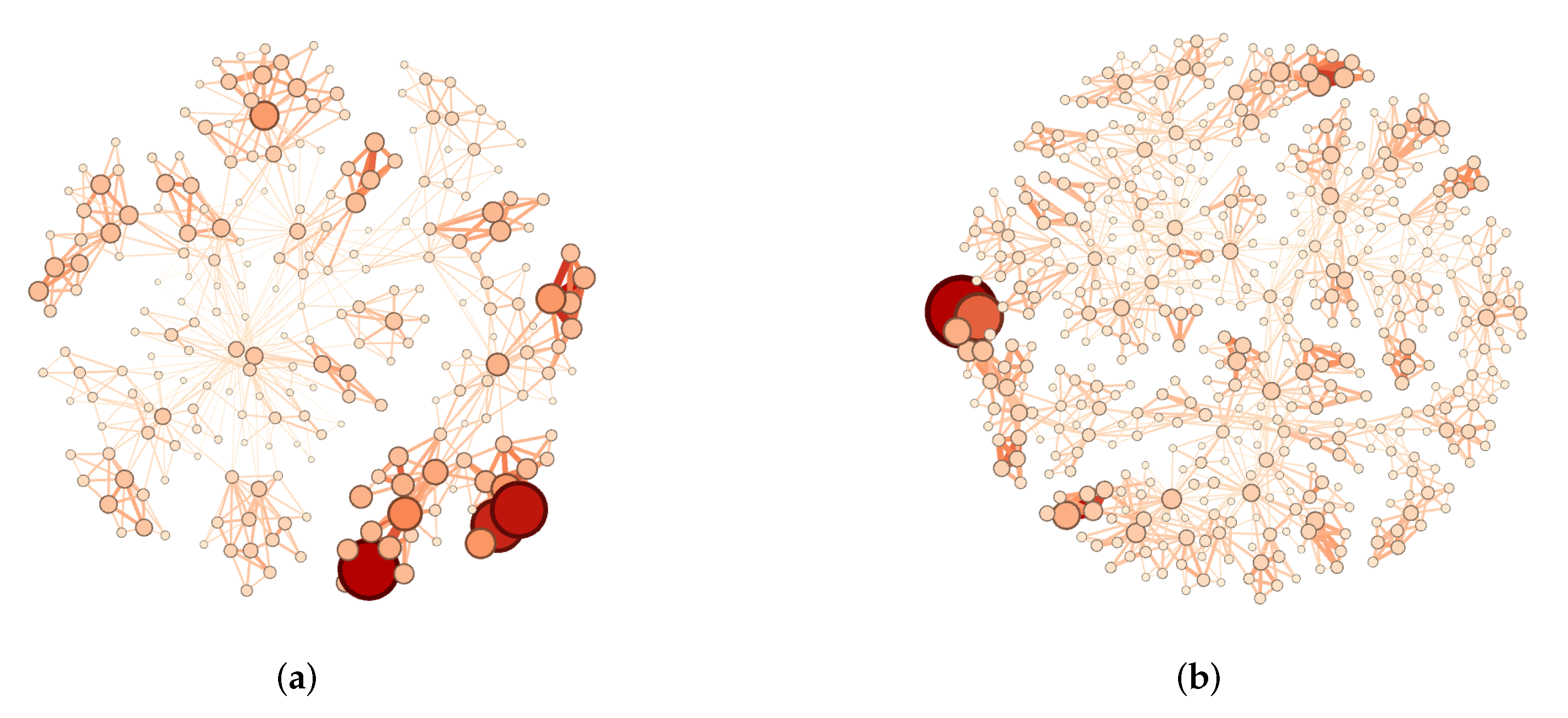
4.1. Quantifying Risk Propagation Flow

As the representatives of emerging and mature markets, Chinese and American stock markets are two typical complex financial networks. Based on the historical data of the components of the S&P500 and HS300 Indices, we calculated the risk propagation flow through all nodes and links, i.e., $F_i$ and $F_{ij}$, for each market. For simplicity, here, we take $B=1$ and $R=1$. The larger the risk propagation flow of a node (link), the more important the corresponding individual stock (interaction between the two stocks) in the information dissemination of the entire market. Thus, we can identify the influential nodes and links in the propagation of information, which may be applicable to portfolio optimization and risk management.

The results for the HS300 market and the S&P500 market are displayed in the Figure 1. There are 483 nodes and 1443 links in the S&P500 risk propagation flow network and 240 nodes and 714 links in the HS300 network. The nodes correspond to individual stocks, and the links represent the risk propagation flow between two stocks. In both markets, a few influential nodes play dominant roles in the risk propagation flow networks.

We sorted the nodes and links of different networks according to the size of risk propagation flow and list the top 10 nodes and links in

Table 1. This table lists the stock tick names corresponding to the top 10 nodes (links) of risk propagation flow networks, ranked by the size of $F_i$($F_{ij}$) for the S&P500 market and HS300 market. For simplicity, here, we take $B=1$ and $R=1$.

Market	Top 10 Nodes	Top 10 Links
S&P500	CAG.N CPB.N DG.N MNST.O AMGN.O GIS.N K.N REGN.O MSFT.O ABT.N	CZR.O ↔ VFC.N CZR.O ↔ SPGI.N CNP.N ↔ CZR.O AME.N ↔ PM.N FITB.O ↔ IQV.N PM.N ↔ TXT.N CNP.N ↔ VFC.N BXP.N ↔ FITB.O CZR.O ↔ DHR.N BXP.N ↔ IQV.N
HS300	002773.SZ 600521.SH 002555.SZ 600763.SH 002624.SZ 600196.SH 300498.SZ 002008.SZ 600436.SH 603939.SH	002714.SZ ↔ 300498.SZ 000876.SZ ↔ 300498.SZ 002311.SZ ↔ 300498.SZ 002157.SZ ↔ 300498.SZ 600196.SH ↔ 600521.SH 600196.SH ↔ 601607.SH 002773.SZ ↔ 600079.SH 600763.SH ↔ 603939.SH 000876.SZ ↔ 002714.SZ 002773.SZ ↔ 600763.SH

. For the HS300 market, the top 10 nodes mainly came from the business sectors—healthcare, information technology, and consumer staples—and most of the top 10 links were found within or between the healthcare and consumer staples sectors. For the S&P500 market, the top 10 nodes were mainly distributed in the business sectors—consumer staples, healthcare, consumer discretionary, and information technology—and most of the top 10 links were found within the business sectors—consumer discretionary, finance, utilities, consumer staples, etc. The distribution of the top 10 nodes for the two markets was similar, while the top 10 links in the S&P500 market were much more dispersed than those in the HS300 market because the American market, as a mature market, has better risk diversification.

To understand the spatiotemporal patterns of risk propagation in complex financial networks, we first investigated the dependence of $F_i$ on the degree distribution of the network by linking it with the weighted degrees of all nodes $S_i={\sum }_{j=1}^{N}Aij$. Next, we focused on the dependence of the individual response time ${\tau }_i$ on the weighted degree $S_i$. As displayed as triangles in Figure 2a,c, $F_i$ positively scales with $S_i$, and as shown as triangles in Figure 2b,d, ${\tau }_i$ negatively scales with $S_i$. In brief, hub nodes (high-degree nodes) played a more important role in risk propagation across the network and respond rapidly, indicating a degree-driven effect. We also linked $F_{ij}$ with the product of i and j’s weighted degree, and the results are listed in Supplementary Material S1. The links first exhibited a link-driven effect and, then, an anti-link-driven effect as $S_i{S}_j$ increased.

As mentioned above, a susceptible node may become infected through interaction with an infected node at a rate R. An infected node recovers at a rate B, becoming susceptible again. Analogically, a stock is infected if the stock is exposed to a risk, and the remaining stocks that have not yet been exposed to a risk are considered susceptible. We further investigated how the infection rate R and the recovery rate B influence the risk propagation flow of complex financial networks. Varying the dynamic parameters R and B from 0 to 1, we investigated the spatiotemporal patterns of the risk propagation flow for the S&P500 and HS300 markets. As displayed in Figure 2, the spatiotemporal patterns remained qualitatively consistent for different R and B, i.e., the nodes exhibit a degree-driven effect. In contrast, spatiotemporal patterns were quantitatively inconsistent for different R and B. As shown in Figure 2a–d, when the recovery rate R decreased, two effects occurred: (i) $F_i$ of the hubs increased, indicating that the nodes tended to be more degree-driven as R decreased; (ii) ${\tau }_i$ of the hubs also increased as R decreased, weakening the degree-driven effect of nodes. Figure 2e–h demonstrate that $F_i$ and ${\tau }_i$ of the hubs both increased, meaning that the degree-driven effect also had two effects as the recovery rate B increased. The impacts of these two dynamic parameters on the degree-driven effect of the nodes were almost opposite.

As reported in [38], on average, risk propagation flow and the node degree obey the relationship $F_i\sim S_i^{\omega }$, and the contribution of $A_{ij}$ link to $Fij$ follows $Fij\sim A_{ij}{S}_i^{\omega -1}{S}_j^{\omega -1}$. For the SIS model of epidemic spread, $\omega =0$ [38]. In this case, $F_i$ is independent of $S_i$, which represents homogeneous flow. Based on linear response theory, ${\tau }_i$ is linked with $S_i$ through the relationship ${\tau }_i\sim S_i^{\theta }$[29]. In other words, ${\tau }_i$ is determined by the interaction between topology $S_i$ and dynamics $\theta$. $\theta$ was determined to be −1 for the SIS model here [29]. However, our empirical results for financial networks were slightly different from the theoretical derivation in References [29,38], which may arise from the complexity of financial networks, such as an obvious community structure and frequent large fluctuations. In future research, we can determine the values of these two parameters based on data from the real market to describe the risk propagation flow of complex financial networks more accurately.

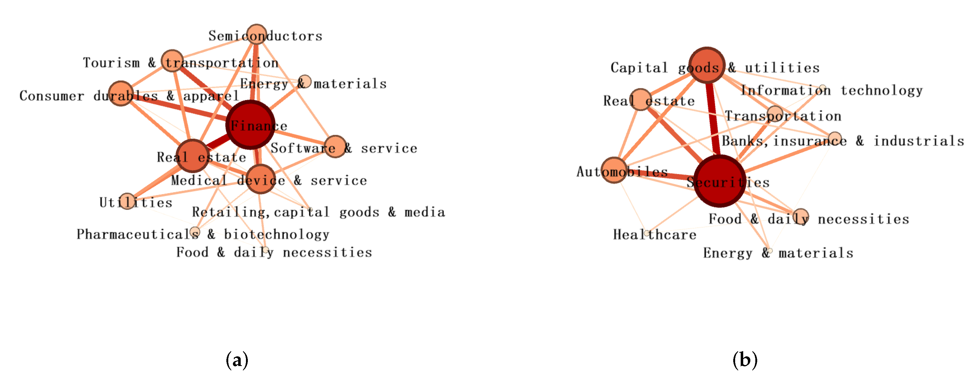
4.2. Risk Propagation Flow of Communities

A distinctive feature of complex financial networks is the existence of community structures. A community is a group of nodes linked with high-density internal edges, which often corresponds to different business sectors in financial markets. Therefore, when calculating risk propagation flow, we need to consider the influence of community structure. We first detected the communities in the sector mode and, then, characterized the risk propagation flow between and within different communities of the complex financial networks.

The Wishart matrix is $C_{ij}$ of N non-correlated time series with length L [83,84]. In the constraints of $N>>1$, $L>>1$, and $Q=L/N\ge 1$, the probability distribution of the eigenvalue $\lambda$ is given by

$$P_{rm}\left(\lambda \right)=\frac{Q}{2\pi }\frac{\sqrt{({\lambda }_{max}^{ran}-\lambda )({\lambda }_{min}^{ran}-\lambda )}}{\lambda }.$$

(11)

The upper and lower bounds of $\lambda$ are

$${\lambda }_{max\left(min\right)}^{ran}={[1\pm 1/\sqrt{Q}]}^2,$$

(12)

Based on the RMD method, we decompose $C_{ij}$ into N-dimensional orthogonal eigenmodes:

$$C_{ij}={\Sigma }_{\alpha =1}^N{\lambda }_{\alpha }{C}_{ij}^{\alpha },C_{ij}^{\alpha }=u_i^{\alpha }{u}_j^{\alpha },$$

(13)

where ${\lambda }_{\alpha }$ is the $\alpha$-th largest eigenvalue, $u_i^{\alpha }$ is the i-th component in the eigenvector of ${\lambda }_{\alpha }$, and $C_{ij}^{\alpha }$ represents the cross-correlation in the $\alpha$-th eigenmode [45,46,47]. According to the size of the eigenvalue ${\lambda }_{\alpha }$, the eigenmodes of real financial markets can be divided into three categories: market mode, sector mode, and random mode [43,44]. For the market mode, $C_{ij}^{mar}={\Sigma }_{\alpha =1}^{mode}{C}_{ij}^{\alpha }{\lambda }_{\alpha }$, which represents the global price movement of the entire market. The sector mode corresponds to the local price motion of business sectors, $C_{ij}^{sec}={\Sigma }_{\alpha =1}^{n-1}{C}_{ij}^{\alpha }{\lambda }_{\alpha }$. Here, ${\lambda }_{\alpha }>{\lambda }_{max}^{ran}$, where ${\lambda }_{max}^{ran}$ is the upper bound of the Wishart matrix [83,84]. n is the number of large eigenvalues exceeding ${\lambda }_{max}^{ran}$. For the random mode, we take $C_{ij}^{ranc}={\Sigma }_{\alpha =n}^{N-1}{C}_{ij}^{\alpha }{\lambda }_{\alpha }$. The random mode contains the non-stationary random background of complex financial systems.

Taking the absolute values of the negative matrix elements, we then generated the PMFG graph $A_{sector,ij}$ from $|C_{sector,ij}|$ [44,77,85]. Next, the community structure was extracted in the Gephi software [86]. After removing the non-stationary random background, we can see the community structure more clearly, and the sector mode further removed the influence of the macro changes of the entire market on the network, allowing us to see the local interactions of communities. Lastly, we characterized the risk propagation flow between and within different communities of the complex financial networks.

The risk propagation flow within communities for the S&P500 market and the HS300 market is displayed in Figure 3. Additionally, the risk propagation flow in each community for the two markets are is displayed in Supplementary Material S1. There are 12 communities and 10 communities for the S&P500 network and the HS300 network. The larger the risk propagation flow of a node (link), the more important the corresponding community (interaction between the two communities) in the information dissemination of the entire market is. For the S&P500 market, the finance community plays a dominant role and the real estate, medical device and service, software and service, and consumer durables and apparel communities play relatively important roles. In contrast, for the HS300 market, the securities community plays a dominant role, followed by the capital goods and utilities, real estate, and automobile communities.

As shown in

Table 2. This table lists the community name, the stock tick name corresponding to the top 1 node, the node/stock number, and the weight of the top 10% stocks’ $F_i$ in each community for the S&P500 market and the HS300 market.

Market	Community Name	Top 1 Node	Nodes No.	Weight
S&P500	Medical device and service	BXP.N	59	27.75%
	Finance	LNC.N	40	22.81%
	Food and daily necessities	CAG.N	37	29.42%
	Consumer durables and apparel	GPS.N	14	25.18%
	Pharmaceuticals and biotechnology	LLY.N	28	23.84%
	Energy and materials	CTSH.O	27	21.30%
	Retailing, capital goods, and media	DLTR.O	27	25.02%
	Software and service	AJG.N	63	30.42%
	Tourism and transportation	PENN.O	44	28.43%
	Utilities	AEE.N	75	32.52%
	Real estate	ITW.N	48	25.74%
	Semiconductors	AMAT.O	21	25.51%
HS300	Securities	601211.SH	22	26.39%
	Food and daily necessities	600050.SH	25	24.35%
	Healthcare	600763.SH	28	27.90%
	Energy and materials	000876.SZ	29	33.58%
	Real estate	002271.SZ	14	24.43%
	Information technology	600584.SH	35	27.40%
	Transportation	601021.SH	15	37.20%
	Capital goods	601618.SH	15	21.82%
	Automobiles	000625.SZ	11	24.43%
	Banks, insurance, and industrials	601818.SH	46	27.07%

, the weight of $F_i$ for the top $10\%$ nodes in each community ranges from $21.30\%$ to $32.52\%$ and from $21.82\%$ to $37.20\%$ for the S&P500 market and the HS300 market, respectively, and the average weights of $F_i$ for the top $10\%$ nodes were $26.49\%$ and $27.46\%$ for the S&P500 market and the HS300 market, respectively. Overall, about $30\%$ of the total risk propagation flow $F_i$ can be explained by the top $10\%$ nodes. The high proportions indicate that the influential nodes in each community play very important roles for both the HS300 market and the S&P500 market. Hence, we may control the risk propagation flow of each community by controlling a few influential nodes of the community and, in turn, the whole network. Potentially, the results can help us build a diversified portfolio in order to manage financial risk.

4.3. Risk Propagation Flow in Extreme Market States

Frequent large fluctuations are another typical characteristic of complex financial network dynamics. A large fluctuation is identified when the volatility is sufficiently large compared with the average one [51].

First, we filtered out large fluctuations in extreme market states by taking different thresholds. For two tails, we assigned $r\left(t^{\prime }\right)=0$ for $\left|r\right(t^{\prime }\left)\right|<\sigma$, where $\sigma$ is the threshold. For the negative (positive) tail, we used $r\left(t^{\prime }\right)=0$ for $r\left(t^{\prime }\right)>-\sigma$ ($r\left(t^{\prime }\right)<\sigma$). Then, we calculated the cross-correlation matrix $C_{ij}$ of $r\left(t^{\prime }\right)$[73,74,75,76]. Then, we pruned the modified cross-correlation matrix $|C_{ij}^{\sigma ,tail}|$ with the PMFG method and generated the threshold PMFG graph $A_{ij}^{\sigma ,tail}$.

Thus, threshold risk propagation flow networks were constructed from the threshold PMFG graph $A_{ij}^{\sigma ,T}$. As shown in Figure 4a–d, $F_i$ positively scaled with $S_i$, and ${\tau }_i$ negatively scaled with $S_i$, i.e., the nodes exhibited a degree-driven effect. When the threshold $\sigma$ increased, two effects were observed: (i) the $F_i$ of the hubs increased, indicating that the nodes tended to be more degree-driven; (ii) the ${\tau }_i$ of the hubs also increased, weakening the degree-driven effect of the nodes. The former effect was stronger by comparison. Therefore, hub nodes were more dominant in extreme market states, indicating that we may achieve better control using hub nodes in these cases.

Furthermore, we distinguished between crashes and bubbles and calculated the risk propagation flow with the threshold PMFG graph $A_{ij}^{\sigma ,N}$ and $A_{ij}^{\sigma ,P}$. As shown in Figure 4e–h, $F_i$ and ${\tau }_i$ of the hubs both increased in the order of two tails, the negative tail, and then, the positive tail. The hub nodes were more dominant, on the one hand, but responded more slowly, on the other hand, during bubbles than during crashes. The dependence of the link $F_{ij}$ on the product of i and j’s weighted degree is listed in Supplementary Material S1.

5. Conclusions

To explore the spatiotemporal patterns of risk propagation in complex financial networks, we combined the SIS infectious disease model with empirical networks. We revealed that hub nodes (high-degree nodes) play important roles in risk propagation across the network and respond rapidly, exhibiting a degree-driven effect. Moreover, we investigated the influence of two key dynamic parameters. The impacts of the two dynamic parameters on the degree-driven effect of the nodes were almost opposite.

Furthermore, we explored the impacts of two typical characteristics of complex financial systems—the existence of community structures and frequent large fluctuations—on risk propagation flow. First, we characterized the risk propagation flow between and within different communities of the complex financial networks. About $30\%$ of the total risk propagation flow of each community can be explained by the top $10\%$ nodes. Thus, we can control the risk propagation flow of each community by controlling a few influential nodes in each community and, in turn, control the whole network. Then, we classified different categories of large fluctuations with the threshold method and explored the risk propagation flow in extreme market states. As the threshold increased, the degree-driven effect of the nodes became greater. In other words, hub nodes become more dominant in extreme market states, indicating that better control may be achieved by hub nodes in these cases.

The results shed light on the underlying mechanisms of risk propagation flow in complex financial networks, answering the questions about which nodes are more important in the risk propagation process and which nodes have a shorter response time. One limitation of our work is that, although the SIS model is an appropriate approximation to describe the risk propagation process of the financial system for now, it is not very accurate. In the future, we can replace it with a more accurate dynamic equation of the financial system. Moreover, we can design a risk management scheme based on our results and control the influential nodes to slow down or curb the spread of financial risk in the whole network. New methods may also be developed and applied to portfolio optimization based on our results.

References

1. Strogatz, S.H. Exploring complex networks. Nature 2001, 410, 268–276. [Google Scholar] [CrossRef] [Green Version]
2. Albert, R.; Barabási, A.L. Statistical mechanics of complex networks. Rev. Mod. Phys. 2002, 74, 47–97. [Google Scholar] [CrossRef] [Green Version]
3. Drogovtsev, S.N.; Mendez, J.F.F. Evolution of Networks: From Biological Nets to the Internet and WWW; Oxfrod University Press: New York, NY, USA, 2003. [Google Scholar]
4. Caldarelli, G. Scale-Free Networks: Complex Webs in Nature and Technology; Oxfrod University Press: New York, NY, USA, 2007. [Google Scholar]
5. Newman, M.E.J. Networks: An Introduction; Oxford University Press: New York, NY, USA, 2010. [Google Scholar]
6. Girvan, M.; Newman, M.E.J. Community structure in social and biological networks. Proc. Natl. Acad. Sci. USA 2002, 99, 7821–7826. [Google Scholar] [CrossRef] [Green Version]
7. Palla, G.; Derenyi, I.; Farkas, I.; Vicsek, T. Uncovering the overlapping community structure of complex networks in nature and society. Nature 2005, 435, 814–818. [Google Scholar] [CrossRef] [Green Version]
8. Zhang, J.; Cao, X.B.; Du, W.B.; Cai, K.Q. Evolution of Chinese airport network. Phys. A 2010, 389, 3922–3931. [Google Scholar] [CrossRef]
9. Du, W.B.; Zhou, X.L.; Lordand, O.; Wang, Z.; Zhao, C.; Zhu, Y.B. Analysis of the chinese airline network as multi-layer networks. Transp. Res. E Logist. Transp. Rev. 2016, 89, 108–116. [Google Scholar] [CrossRef] [Green Version]
10. Lu, L.Y.; Chen, D.B.; Ren, X.L.; Zhang, Q.M.; Zhou, T. Vital nodes identification in complex networks. Phys. Rev. 2016, 650, 1–63. [Google Scholar]
11. Jiang, X.F.; Xiong, L.; Bai, L.; Zhao, N.; Zhang, J.; Xia, K.; Deng, K.; Zheng, B. Quantifying the social structure of elites in ancient China. Phys. A 2021, 573, 125976. [Google Scholar] [CrossRef]
12. Newman, M.E.J.; Girvan, M. Finding and evaluating community structure in networks. Phys. Rev. E 2003, 69, 026113. [Google Scholar] [CrossRef] [PubMed] [Green Version]
13. Fortunato, S. Community detection in graphs. Phys. Rep. 2010, 486, 75–174. [Google Scholar] [CrossRef] [Green Version]
14. Fortunato, S.; Latora, V.; Marchiori, M. Method to find community structures based on information centrality. Phys. Rev. E 2004, 70, 056104. [Google Scholar] [CrossRef] [PubMed]
15. Sun, P.G.; Gao, L.; Yang, Y. Maximizing modularity intensity for community partition and evolution. Inf. Sci. 2013, 236, 83–92. [Google Scholar] [CrossRef]
16. Rosvall, M.; Bergstrom, C.T. Maps of random wakls on complex networks reveal community structure. Proc. Natl. Acad. Sci. USA 2007, 105, 1118–1123. [Google Scholar] [CrossRef] [PubMed] [Green Version]
17. Radicchi, F.; Castellano, C.; Cecconi, F.; Loreto, V.; Parisi, D. Defining and identifying communities in networks. Proc. Natl. Acad. Sci. USA 2004, 101, 2658–2663. [Google Scholar] [CrossRef] [Green Version]
18. Sun, P.G.; Gao, L.; Han, S. Identification of overlapping and non-overlapping community structure by fuzzy clustering. Inf. Sci. 2011, 181, 1060–1071. [Google Scholar] [CrossRef]
19. Lizier, J.T.; Prokopenko, M.; Zomaya, A.Y. Local information transfer as a spatiotemporal filter for complex systems. Phys. Rev. E 2008, 77, 026110. [Google Scholar] [CrossRef] [Green Version]
20. Telesford, Q.K.; Simpson, S.L.; Burdette, J.H.; Hayasaka, S.; Laurienti, P.J. The brain as a complex system: Using network science as a tool for understanding the brain. Brain Connect. 2011, 1, 295–308. [Google Scholar] [CrossRef] [Green Version]
21. Kwon, O.; Yang, J.S. Information flow between stock indices. Europhys. Lett. 2008, 82, 68003. [Google Scholar] [CrossRef] [Green Version]
22. Allali, A.; Oueslati, A.; Trabelsi, A. Detection of Information Flow in Major International Financial Markets by Interactivity Network Analysis. Asia-Pac. Financ. Markets 2011, 18, 319–344. [Google Scholar] [CrossRef]
23. Saito, K.; Kimura, M.; Ohara, K.; Motoda, H. Detecting critical links in complex network to maintain information flow/reachability. In Proceedings of the Pacific Rim International Conference on Artificial Intelligence, Phuket, Thailand, 22–26 August 2016; Springer: Cham, Switzerland, 2016; p. 419. [Google Scholar]
24. Korbel, J.; Jiang, X.F.; Zheng, B. Transfer Entropy between Communities in Complex Financial Networks. Entropy 2019, 21, 1124. [Google Scholar] [CrossRef] [Green Version]
25. Min, J.; Zhu, J.J.; Yang, J.B. The Risk Monitoring of the Financial Ecological Environment in Chinese Outward Foreign Direct Investment Based on a Complex Network. Sustainability 2020, 12, 9456. [Google Scholar] [CrossRef]
26. Barzel, B.; Barabási, A.L. Universality in network dynamics. Nat. Phys. 2013, 9, 673–681. [Google Scholar] [CrossRef] [Green Version]
27. Gao, J.; Barzel, B.; Barabási, A.L. Universal resilience patterns in complex networks. Nature 2016, 530, 307312. [Google Scholar] [CrossRef] [PubMed]
28. Bai, L.; Xiong, L.; Zhao, N.; Xia, K.; Jiang, X.F. Dynamical structure of social map in ancient China. Phys. A 2022, 607, 128209. [Google Scholar] [CrossRef]
29. Hens, C.; Harush, U.; Haber, S.; Cohen, R.; Barzel, B. Spatiotemporal signal propagation in complex networks. Nat. Phys. 2019, 15, 403–412. [Google Scholar] [CrossRef]
30. Liu, Y.Y.; Slotine, J.J.; Barabási, A.L. Controllability of complex networks. Nature 2011, 473, 167–173. [Google Scholar] [CrossRef] [PubMed]
31. Yan, G.; Ren, J.; Lai, Y.C.; Lai, C.H.; Li, B. Controlling complex networks: How much energy is needed? Phys. Rev. Lett. 2012, 108, 218703. [Google Scholar] [CrossRef] [Green Version]
32. Wang, W.X.; Ni, X.; Lai, Y.C.; Grebogi, C. Optimizing controllability of complex networks by small structural perturbations. Phys. Rev. E 2012, 85, 026115. [Google Scholar] [CrossRef] [PubMed] [Green Version]
33. Cornelius, S.P.; Kath, W.L.; Motter, A.E. Realistic control of network dynamics. Nat. Commun. 2013, 4, 1942. [Google Scholar] [CrossRef] [Green Version]
34. Nacher, J.C.; Akutsu, T. Structurally robust control of complex networks. Phys. Rev. E 2015, 91, 012826. [Google Scholar] [CrossRef] [Green Version]
35. Onnela, J.P. Flow of control in networks. Science 2014, 343, 1325. [Google Scholar] [CrossRef]
36. Ruths, J.; Ruths, D. Control profiles of complex networks. Science 2014, 343, 1373–1376. [Google Scholar] [CrossRef]
37. Sun, P.G. Controllability and modularity of complex networks. Inf. Sci. 2015, 325, 20–32. [Google Scholar] [CrossRef]
38. Harush, U.; Barzel, B. Dynamic patterns of information flow in complex networks. Nat. Commun. 2017, 8, 2181. [Google Scholar] [CrossRef] [PubMed] [Green Version]
39. Reichardt, J.; Bornholdt, S. Statistical mechanics of community detection. Phys. Rev. E 2006, 74, 016110. [Google Scholar] [CrossRef] [PubMed] [Green Version]
40. Newman, M.E.J. Modularity and community structure in networks. Proc. Natl. Acad. Sci. USA 2006, 103, 8577–8582. [Google Scholar] [CrossRef] [PubMed] [Green Version]
41. Li, H.J.; Wang, Y.; Wu, L.Y.; Liu, Z.P.; Chen, L.N.; Zhang, X.S. Community structure detection based on Potts model and network’s spectral characterization. Europhys. Lett. 2012, 97, 48005. [Google Scholar] [CrossRef]
42. Pan, R.K.; Sinha, S. Collective behavior of stock price movements in an emerging market. Phys. Rev. E 2007, 76, 046116. [Google Scholar] [CrossRef] [Green Version]
43. Jiang, X.F.; Zheng, B. Anti-correlation and subsector structure in financial systems. Europhys. Lett. 2012, 97, 48006. [Google Scholar] [CrossRef] [Green Version]
44. Jiang, X.F.; Chen, T.T.; Zheng, B. Structure of local interactions in complex financial dynamics. Sci. Rep. 2014, 4, 5321. [Google Scholar] [CrossRef] [PubMed] [Green Version]
45. Plerou, V.; Gopikrishnan, P.; Rosenow, B.; Amaral, L.A.N.; Guhr, T.; Stanley, H.E. Random matrix approach to cross-correlations in financial data. Phys. Rev. E 2002, 65, 066126. [Google Scholar] [CrossRef] [PubMed]
46. Utsugi, A.; Ino, K.; Oshikawa, M. Random matrix theory analysis of cross-correlations in financial markets. Phys. Rev. E 2004, 70, 026110. [Google Scholar] [CrossRef] [PubMed] [Green Version]
47. Pan, R.K.; Sinha, S. Self-organization of price fluctuation distribution in evolving markets. Europhys. Lett. 2007, 77, 58004. [Google Scholar] [CrossRef] [Green Version]
48. Sornette, D. Critical market crashes. Phys. Rep. 2003, 378, 1. [Google Scholar] [CrossRef] [Green Version]
49. Mu, G.H.; Zhou, W.X. Relaxation dynamics of aftershocks after large volatility shocks in the ssec index. Phys. A 2008, 387, 5211. [Google Scholar] [CrossRef] [Green Version]
50. Sornette, D.; Woodard, R.; Zhou, W.X. The 2006–2008 oil bubble: Evidence of speculation, and prediction. Phys. A 2009, 388, 1571–1576. [Google Scholar] [CrossRef] [Green Version]
51. Jiang, X.F.; Chen, T.T.; Zheng, B. Time-reversal asymmetry in financial systems. Phys. A 2013, 392, 5369. [Google Scholar] [CrossRef] [Green Version]
52. Nobi, A.; Maeng, S.E.; Ha, G.G.; Lee, J.W. Effects of global financial crisis on network structure in a local stock market. Phys. A 2014, 03, 083. [Google Scholar] [CrossRef]
53. Daron, A.; Asuma, O.; Alireza, T.S. Systemic risk and stability in financial networks. Am. Econ. Rev. 2015, 105, 564. [Google Scholar]
54. Bardoscia, M.; Battiston, S.; Caccioli, F.; Caldarelli, G. Pathways towards instability in financial networks. Nat. Commun. 2017, 8, 14416. [Google Scholar] [CrossRef] [Green Version]
55. Battiston, S.; Caldarelli, G.; May, R.; Roukny, T.; Stiglitz, J.E. The price of complexity in financial networks. Proc. Natl. Acad. Sci. USA 2016, 113, 10031. [Google Scholar] [CrossRef] [PubMed]
56. Chen, T.T.; Zheng, B.; Li, Y.; Jiang, X.F. Temporal correlation functions of dynamic systems in non-stationary states. New J. Phys. 2018, 20, 073005. [Google Scholar] [CrossRef]
57. Samanidou, E.; Zschischang, E.; Stauffer, D.; Lux, T. Agent-based models of financial markets. Rep. Prog. Phys. 2007, 70, 409. [Google Scholar] [CrossRef] [Green Version]
58. Shive, S. An Epidemic Model of Investor Behavior. J. Financ. Quant. Anal. 2010, 45, 169. [Google Scholar] [CrossRef] [Green Version]
59. Mantegna, R.N.; Kertész, J. Focus on statistical physics modeling in economics and finance. New J. Phys. 2011, 13, 25011. [Google Scholar] [CrossRef]
60. Chakraborti, A.; Toke, I.M.; Patriarca, M.; Abergel, F. Econophysics review: II. Agent-based models. Quant. Financ. 2011, 11, 1013. [Google Scholar] [CrossRef] [Green Version]
61. Sornette, D. Physics and financial economics (1776–2014): Puzzles, Ising and agent-based models. Rep. Prog. Phys. 2014, 77, 62001. [Google Scholar] [CrossRef]
62. Demiris, N.; Kypraios, T.; Smith, L.V. On the epidemic of financial crises. J. R. Statist. Soc. A 2014, 177, 697. [Google Scholar] [CrossRef] [Green Version]
63. Balci, M.A. Fractional virus epidemic model on financial networks. Open Math. 2016, 14, 1074. [Google Scholar] [CrossRef] [Green Version]
64. Martikainen, T.; Puttonen, V. On the informational flow between financial markets: International evidence from thin stock and stock index futures markets. Econ. Lett. 1992, 38, 213–216. [Google Scholar] [CrossRef]
65. Eom, C.; Jung, W.S.; Choi, S.; Oh, G.; Kim, S. Effects of time dependency and efficiency on information flow in financial markets. Phys. A Stat. Mech. Its Appl. 2008, 387, 5219–5224. [Google Scholar] [CrossRef] [Green Version]
66. Kim, Y.; Kim, J.; Yook, S.H. Information transfer network of global market indices. Phys. A Stat. Mech. Its Appl. 2015, 430, 39–45. [Google Scholar] [CrossRef]
67. Xie, W.J.; Yong, Y.; Wei, N.; Yue, P.; Zhou, W.X. Identifying states of global financial market based on information flow network motifs. N. Am. J. Econ. Financ. 2021, 58, 101459. [Google Scholar] [CrossRef]
68. Park, S.; Jang, K.; Yang, J.S. Information flow between bitcoin and other financial assets. Phys. A Stat. Mech. Its Appl. 2021, 566, 125604. [Google Scholar] [CrossRef]
69. Teng, Y.; Shang, P. Transfer entropy coefficient: Quantifying level of information flow between financial time series. Phys. A Stat. Mech. Its Appl. 2017, 469, 60–70. [Google Scholar] [CrossRef]
70. Dimpfl, T.; Peter, F.J. The impact of the financial crisis on transatlantic information flows: An intraday analysis. J. Int. Financ. Mark. Institutions Money 2014, 31, 1–13. [Google Scholar] [CrossRef] [Green Version]
71. Yang, H.; Qi, S.; Zhang, Z.; Koslowsky, D. A model of information diffusion with asymmetry and confidence effects in financial markets. N. Am. J. Econ. Financ. 2021, 57, 101404. [Google Scholar] [CrossRef]
72. Lu, J.; Chen, X.; Liu, X. Stock market information flow: Explanations from market status and information-related behavior. Phys. A Stat. Mech. Its Appl. 2018, 512, 837–848. [Google Scholar] [CrossRef]
73. Shen, J.; Zheng, B. Cross-correlation in financial dynamics. Europhys. Lett. 2009, 86, 48005. [Google Scholar] [CrossRef] [Green Version]
74. Podobnik, B.; Wang, D.; Horvatic, D.; Grosse, I.; Stanley, H.E. Time-lag cross-correlations in collective phenomena. Europhys. Lett. 2010, 90, 68001. [Google Scholar] [CrossRef] [Green Version]
75. Laloux, L.; Cizeau, P.; Bouchaud, J.P.; Potters, M. Noise dressing of financial correlation matrices. Phys. Rev. Lett. 1999, 83, 1467. [Google Scholar] [CrossRef] [Green Version]
76. Gopikrishnan, P.; Rosenow, B.; Plerou, V.; Stanley, H.E. Quantifying and interpreting collective behavior in financial markets. Phys. Rev. E 2001, 64, 035106. [Google Scholar] [CrossRef]
77. Tumminello, M.; Aste, T.; Matteo, T.D.; Mantegna, R.N. A tool for filtering information in complex systems. Proc. Natl. Acad. Sci. USA 2005, 102, 10421. [Google Scholar] [CrossRef] [Green Version]
78. Dodds, P.S.; Watts, D.J. A generalized model of social and biological contagion. J. Theor. Biol. 2005, 232, 587–604. [Google Scholar] [CrossRef] [PubMed] [Green Version]
79. Pastor-Satorras, R.; Vespignani, A. Epidemic spreading in scale-free networks. Phys. Rev. Lett. 2001, 86, 3200. [Google Scholar] [CrossRef] [Green Version]
80. Hufnagel, L.; Brockmann, D.; Geisel, T. Forecast and control of epidemics in a globalized world. Proc. Natl. Acad. Sci. USA 2004, 101, 15124. [Google Scholar] [CrossRef] [PubMed] [Green Version]
81. Matthew, E.; Benjamin, G.; Matthew, O.J. Financial networks and contagion. Am. Econ. Rev. 2014, 104, 3115–3153. [Google Scholar]
82. Barzel, B.; Biham, O. Quantifying the connectivity of a network: The network correlation function method. Phys. Rev. E 2009, 80, 046104. [Google Scholar] [CrossRef] [Green Version]
83. Dyson, F.J. Distribution of eigenvalues for a class of real symmetric matrices. Rev. Mex. Fis. 1971, 20, 231. [Google Scholar]
84. Sengupta, A.M.; Mitra, P.P. Distributions of singular values for some random matrices. Phys. Rev. E 1999, 60, 3389. [Google Scholar] [CrossRef] [Green Version]
85. Rosvall, M.; Bergstrom, C.T. Mapping change in large networks. PLoS ONE 2010, 5, e8694. [Google Scholar] [CrossRef] [PubMed]
86. Bastian, M.; Heymann, S.; Jacomy, M. Gephi: An open source software for exploring and manipulating networks. In Proceedings of the International AAAI Conference on Weblogs and Social Media, San Jose, CA, USA, 17–20 May 2009; Volume 3, p. 361. [Google Scholar]
Figure 1. (a) Risk propagation flow network of the HS300 market. (b) Risk propagation flow network of the S&P500 market. The size of nodes and the width of links represent the F i of a stock and the F i j between two stocks, respectively. For simplicity, here, we take B = 1 and R = 1 .
Applsci 13 01129 g001
Figure 2. Spatiotemporal patterns of risk propagation with different dynamic parameters. We measured the risk propagation flow F i and the local response times τ i of all nodes/links with different dynamic parameters for the S&P500 market and the HS300 market. (a) F i vs. the weighted degree S i for the S&P500 market with different infection rates R. (b) τ i vs. S i for the S&P500 market with different infection rates R. (c) F i vs. S i for the HS300 market with different infection rates R. (d) τ i vs. S i for the HS300 market with different infection rates R. (e) F i vs. S i for the S&P500 market with different recovery rates B. (f) τ i vs. S i for the S&P500 market with different recovery rates B. (g) F i vs. S i for the HS300 market with different recovery rates B. (h) τ i vs. S i for the HS300 market with different recovery rates B.
Applsci 13 01129 g002
Figure 3. (a) Risk propagation flow within communities for the S&P500 market. (b) Risk propagation flow within communities for the HS300 market. The size of the nodes and the width of links denote the F i of a community and the F i j between two communities, respectively.
Applsci 13 01129 g003
Figure 4. Spatiotemporal patterns of risk propagation in extreme market states. We measured the risk propagation flow F i and the local response times τ i of all nodes for the S&P500 market and the HS300 market in extreme market states. For comparison, the results of the original network are displayed in triangles. (a) F i vs. the weighted degree S i for the S&P500 market with different threshold σ for two tails, T. (b) τ i vs. S i for the S&P500 market with different threshold σ for two tails, T. (c) F i vs. S i for the HS300 market with different threshold σ for two tails, T. (d) τ i vs. S i for the HS300 market with different threshold σ for two tails, T. (e) F i vs. S i for the S&P500 market for two tails, T; the negative tail, N; and the positive tail, P. (f) τ i vs. S i for the S&P500 market for two tails, T; the negative tail, N; and the positive tail, P. (g) F i vs. S i for the HS300 market for two tails, T; the negative tail, N; and the positive tail, P. (h) τ i vs. S i for the HS300 market for two tails, T; the negative tail, N; and the positive tail, P. For (ad), σ [ 0.5 , 2 ] , while for (eh), σ = 1.5 .
Applsci 13 01129 g004