Research on Characteristics of Flow Noise and Flow-Induced Noise

Abstract

The noise control of flank array sonar is a primary approach to enhance the sonar detection range. During submarine navigation, hydrodynamic noise is the main noise source in the platform region of the flank array sonar, which includes flow noise and flow-induced noise. Therefore, an in-depth investigation of hydrodynamic noise is necessary. In this paper, we firstly take the teardrop submarine as a computational model to validate the computational method. Afterwards, we numerically simulate the flow and flow-induced noise characteristics for the cylindrical shell model, and investigate differences in noise at different detection points along the X, Y, and Z axes. Finally, experiments are conducted to confirm the accuracy of the simulation results. The research findings reveal that, at the same frequency, flow-induced noise exceeds flow noise, and the noise decreases as the distance between the walls of the cylindrical shell increases. The experimental and simulation results are consistent, suggesting that the selected computational method can precisely simulate the submarine’s noise.

1. Introduction

The flank array sonar is a passive sonar with a large-scale hydrophone base array mounted on the side of a submarine, which can provide remote passive detection, classification, and localization [1]. However, when the submarine is in motion, the noise generated by the interaction between the flow field and the hull can interfere with sonar detection. Consequently, it is of vital significance to investigate the noise characteristics of submarines, mitigate the impact of submarine-generated noise on flank array sonar, and optimize the arrangement of flank array sonar to enhance its anti-noise performance [2].

The noise of the flank array sonar platform is mainly divided into three parts: mechanical noise, propeller noise, and hydrodynamic noise [3]. As a result of the high speed of underwater navigation, as the navigation speed increases, the proportion of hydrodynamic noise gradually increases. Therefore, we focused our research and analysis on hydrodynamic noise. Hydrodynamic noise, as the dominant noise at relatively high navigation speeds, can be divided into flow noise and flow-induced noise [4]. Among them, flow noise is mainly caused by the combination of turbulent boundary layer disturbance outside the structural shell and wall pulsating pressure. On this basis, flow-induced noise is the superposition of structural vibration and noise generated by the interaction between the shell and fluid [5].

In order to achieve a credible study of its underwater performance, a clear understanding of its surrounding flow field must be obtained. The study of flow field in the past was to directly obtain relevant data through underwater experiments, and then to calculate and analyze its structural parameters; however, obtaining data directly through experiments will consume relatively high resources. In recent years, with the development of computational fluid dynamics (CFD) and computational acoustics, it has become possible to study the noise of underwater targets using numerical simulation methods.

Lu et al. [6] computed the flow field of the SUBOFF submarine using Fluent software and then utilized Fluent’s acoustic module to calculate the flow noise. However, due to the inclusion of compact source assumptions, although it accurately calculated far-field acoustic information, it introduced significant errors into the calculations near the submarine’s surface. Zeng [7] employed a combination of computational fluid dynamics and the boundary element method to calculate the flow noise of a fully appended submarine, obtaining the total sound pressure level at characteristic points. Kellett et al. [8] used the k-ε model in conjunction with the FW-H equation to numerically predict the underwater radiated noise of LNG ships. Wang et al. [9] combined Large Eddy Simulation (LES) with the Infinite Element Method (I-FEM) to perform frequency-domain numerical predictions of the flow noise from propellers in uniform flow and the flow noise from submarines. Shi [10] used the SUBOFF scaled model to simulate and model the hull command deck line shape and hull shell thickness. He studied the acoustic radiation characteristics of the hull flow-excited structural vibration under the action of pulsating pressure, but did not conduct a comparison with the flow noise.

While many scholars have conducted research on submarine noise, previous studies on flow-induced noise assumed that structural deformations of the hull during underwater movement could be neglected [11]. However, under the effect of pulsating pressure, the shell still undergoes certain structural displacement changes resulting in vibration noise [12,13]. Therefore, analyzing the flow-induced noise generated during the underwater shell motion based on one-way fluid−structure interaction has significant research value [14,15].

In this study, we not only calculated flow noise, but also computed flow-induced noise, comparing it with flow noise. For submarines, the proportion of sonar array size is small. In the experiment, we need to consider the array size of the hydrophone in combination with the size of the carrier. As the hydrophone is approximated as a straight line in the array direction, we used the cylindrical shell as the model for simulation and experiment. Firstly, we validated the computational methods using a teardrop submarine model. Subsequently, we established a cylindrical shell model to conduct numerical simulations of flow noise and flow-induced noise characteristics. We investigated the differences in noise at various detection points along the X, Y, and Z axes. Lastly, we designed a towing experiment to verify the accuracy of the simulations.

This provides a reference for analyzing the noise characteristics of military vessels and optimizing the arrangement of the flank array sonar. In the next step, a more realistic ship model can be established to calculate the noise distribution in key areas and for verification with the experimental results. Additionally, adjustments to the installation angles and positions of the sonar could be made specifically for noise-prone regions, thereby enhancing the signal-to-noise ratio of the sonar system.

2. Computational Theory

2.1. Flow Noise Calculation Theory

The study of flow noise started with Lighthill’s acoustic analogy theory, which combines acoustic field and flow field calculations to solve flow noise by solving flow field information [16]. Lighthill’s basic equation is as follows:

$$\frac{{\partial }^2{\rho }^{\prime }}{\partial t^2}-c_0^2{\nabla }^2{\rho }^{\prime }=\frac{{\partial }^2{T}_{ij}}{\partial x_i\partial x_j}$$

(1)

where $c_0^{}$ is the speed of sound under isentropic conditions; ${\rho }^{\prime }=\rho -{\rho }_0$, where $\rho$ and ${\rho }^{\prime }$ are the densities of the fluid under disturbed and undisturbed conditions, respectively; $T_{ij}$ is the Lighthill’s stress tensor.

The boundary element method is capable of accurately computing and solving flow noise for complex structures at low frequencies. By utilizing Helmholtz equation in conjunction with the acoustic control equation, the differential equations within the solution domain are transformed into integral equations over the boundary. These integral equations are then discretized into simpler weighted forms using numerical methods [17].

Let ${\widehat{p}}^{\prime }{e}^{i\omega t}=c^2\widehat{\rho }{e}^{i\omega t}=c_0^2{\rho }^{\prime }$, $\widehat{q}=\frac{{\partial }^2{\widehat{T}}_{ij}}{\partial x_i\partial x_j}$, $T_{ij}={\widehat{T}}_{ij}{e}^{i\omega t}$, where $k=\omega /c_0$ is the wave number, the symbol above ${\widehat{p}}^{\prime }$, ${\widehat{\rho }}^{\prime }$ and ${\widehat{T}}_{ij}$ indicates that they are frequency domain variables.

Taking the Fourier transform of Equation (1), we arrive at the following expression:

$${\nabla }^2{p}^{\prime }+k^2{p}^{\prime }=q$$

(2)

For the sake of simplicity, the symbols denoting frequency domain variables have been omitted. In the subsequent text, unless otherwise specified, all variables represent frequency domain quantities. Reference [18] applies a specific treatment to Equation (2), indicating that the sound pressure at the receiving point in the acoustic field needs to satisfy the following formula:

$$C{p}^{\prime }={{\displaystyle \int }}_V{T}_{ij}\frac{{\partial }^{2}G}{\partial y_i\partial y_j}\mathrm{d}V-{{\displaystyle \int }}_{{\mathsf{\Omega }}_a}{p}^{\prime }\frac{\partial G}{\partial n}\mathrm{d}{\mathsf{\Omega }}_a$$

(3)

where $V$ is the volume domain to be solved; ${\mathsf{\Omega }}_a$ is the solid wall surface; $C$ is the surface shape function, taking 0.5 when the receiving point is on the solid surface and 1. when the receiving point is inside the solution domain; $G$ is the Green’s function satisfying $G(\overrightarrow{r},{\overrightarrow{r}}_a)=\frac{e^{-jk\mid \overrightarrow{r}-{\overrightarrow{r}}_a\mid }}{4\pi \mid \overrightarrow{r}-{\overrightarrow{r}}_a\mid }$, where $r_a$ is the sound source point.

In Equation (2), the flow noise $p^{\prime }$ can be decomposed into the sum of hydrodynamic fluctuating pressure $p_h$ and acoustic fluctuating pressure $p_a$, i.e.,

$$p^{\prime }=p_h+p_a$$

(4)

where $p_h$ can be obtained by calculating the flow field, but $p_a$ is unknown. To solve for $p_a$, the integral domain needs to be decomposed. The volume domain is decomposed into $V_1$ and $V_2$, with corresponding boundaries of ${\mathsf{\Omega }}_1$ and ${\mathsf{\Omega }}_2$, respectively. $V_1$ is the volume close to the receiving point $r$, which is only affected by $p_a$; ${\mathsf{\Omega }}_2$ is the remaining volume of the integral domain, where the receiving point $r$ is affected by both $p_a$ and $p_h$. Substituting Equation (4) into (3) and using the approximate formula of Lighthill stress tensor $T_{ij}\approx {\rho }_0{u}_i{u}_j$, we can obtain:

$$C{p}_a=-{{\displaystyle \int }}_{\mathsf{\Omega }}{p}_a\frac{\partial G}{\partial n}\mathrm{d}\mathsf{\Omega }+{{\displaystyle \int }}_{V_2}{\rho }_0{u}_i{u}_j\frac{{\partial }^{2}G}{\partial y_i\partial y_j}\mathrm{d}{V}_1-{{\displaystyle \int }}_{{\mathsf{\Omega }}_2}{p}_h\frac{\partial G}{\partial n}{\mathrm{d}\mathsf{\Omega }}_2$$

(5)

Before solving using the boundary element method, discretization is first performed. For any point $r_a$ on the mesh cell $\mathsf{\Omega }e$, assuming the acoustic pressure satisfies the discrete function:

$$p^{\prime }(r_a)={\displaystyle \sum _{i=1}^{n_e}{N}_i^e(r_a)p_i^{\prime }}$$

(6)

where the local shape function $N_i^e$ takes the value 1 at node $i$ and 0 at other positions; $n_e$ is the number of nodes on mesh cell $\mathsf{\Omega }e$.

Expanding the local shape function $N_i^e$ in Equation (6) to the entire mesh surface $\mathsf{\Omega }$ yields the global shape function $N_i$, which takes the value $N_i^e$ on cell $\mathsf{\Omega }e$ and 0 at other positions, i.e.,

$$p^{\prime }(r_a)=[N_i]\{p_i^{\prime }\}$$

(7)

Equation (5) can be solved using the boundary element method. Substituting (7) into (5) yields the following:

$$C{p}_a=-\{p_{aj}\}{{\displaystyle \int }}_{\mathsf{\Omega }}[N_j]\frac{\partial G}{\partial n}\mathrm{d}\mathsf{\Omega }-\{p_{hk}\}{{\displaystyle \int }}_{{\mathsf{\Omega }}_2}[N_k]\frac{\partial G}{\partial n}{\mathrm{d}\mathsf{\Omega }}_2+Q$$

(8)

where $Q$ represents the volume integral over $T_{ij}$, which can be ignored at low Mach numbers as $T_{ij}$ is small.

Applying Equation (8) to all nodes on the surface mesh $\mathsf{\Omega }$, the final equation for solving flow noise can be obtained as follows:

$$C{p}_{ai}=-[A_{ij}]\{p_{aj}\}-[A_{ik}]\{p_{hk}\}$$

(9)

where:

$$[A_{ij}]={{\displaystyle \int }}_{\mathsf{\Omega }}[N_j]\frac{\partial G(\mathit{r},{\mathit{r}}_j)}{\partial n}\mathrm{d}\mathsf{\Omega }$$

(10)

$$\left[A_{ik}\right]={{\displaystyle \int }}_{{\mathsf{\Omega }}_2}[N_k]\frac{\partial G(\mathit{r},{\mathit{r}}_k)}{\partial n}{\mathrm{d}\mathsf{\Omega }}_2$$

(11)

The original integral equation has now been simplified to an algebraic weighted form. Substituting $p_a$ into Equation (4) gives the flow noise at any point.

2.2. Flow-Induced Noise Calculation Theory

As a result of the flow-induced vibration of the hull surface, the velocity boundary condition needs to be satisfied:

$$v_n=\frac{j}{{\rho }_0\omega }\frac{\partial p}{\partial n}={\overline{v}}_n$$

(12)

Equation (2) is an inhomogeneous Helmholtz equation. According to the superposition principle, its solution can be considered as the superposition of the solution $p_a$ to the homogeneous Helmholtz equation and the solution $p_b$ to the inhomogeneous Helmholtz equation, i.e.,

$$p^{\prime }=p_a+p_b$$

(13)

where $p_b$ is the flow noise without considering fluid−structure coupling, which was solved in the previous section. $p_a$ is the solution to the homogeneous Helmholtz equation satisfying: the following

$${\nabla }^2{p}_a+k^2{p}_a=0$$

(14)

The velocity boundary condition to be satisfied for Equation (14) is as follows:

$$\frac{j}{{\rho }_0\omega }\frac{\partial p_a}{\partial n}=\overline{v_n}-\frac{j}{{\rho }_0\omega }\frac{\partial p_b}{\partial n}$$

(15)

Now, we just need to solve the homogeneous Helmholtz equation. Discretization is first performed. For any point on mesh cell ${\mathsf{\Omega }}_{ae}$, assuming the acoustic pressure and velocity have the following discrete functions, respectively:

$$p({\overrightarrow{r}}_a)={\displaystyle \sum }_{i=1}^{n_e}{N}_i^e({\overrightarrow{r}}_a)p_i$$

(16)

$${\nu }_n({\overrightarrow{r}}_a)={\displaystyle \sum }_{i=1}^{n_e}{N}_i^e({\overrightarrow{r}}_a){\nu }_{ni}$$

(17)

where the shape function $N_i^e$ takes the value 1 at node $i$ and 0 at other positions; $n_e$ is the number of nodes on cell ${\mathsf{\Omega }}_{ae}$. The shape functions $N_i^e$ in Equations (16) and (17) are only the local shape functions defined on cell ${\mathsf{\Omega }}_{ae}$. Expanding them to the entire mesh surface ${\mathsf{\Omega }}_a$ yields the global shape functions $N_i$, which takes the value $N_i^e$ on cell ${\mathsf{\Omega }}_{ae}$ and 0 at other positions, i.e.,

$$p({\overrightarrow{r}}_a)=[N_i]\{p_i\}$$

(18)

$${\nu }_n({\overrightarrow{r}}_a)=[N_i]\{{\nu }_{ni}\}$$

(19)

According to the theory of boundary elements, the solution satisfying Equation (14), velocity boundary condition (15), and the Sommerfeld radiation condition is as follows:

$$C{p}_a(\overrightarrow{r})={{\displaystyle \int }}_{\mathsf{\Omega }}(p({\overrightarrow{r}}_a)\frac{\partial G(\overrightarrow{r},{\overrightarrow{r}}_a)}{\partial n}-G(\overrightarrow{r},{\overrightarrow{r}}_a)\frac{\partial p({\overrightarrow{r}}_a)}{\partial n})\mathrm{d}\mathsf{\Omega }$$

(20)

where the coefficients $C$ take the following values:

$$C=\left\{\begin{array}{l}0.5\\ 1\\ 0\end{array}\right.\begin{array}{cc}& \overrightarrow{r}\in \mathsf{\Omega }\\ & \overrightarrow{r}\in V\mid \mathsf{\Omega }\\ & \overrightarrow{r}\notin V\end{array}$$

(21)

In Equation (20), letting an arbitrary point $\overrightarrow{r}$ in the acoustic field be at node ${\overrightarrow{r}}_b$, then

$$[A_b]\{p_{ai}\}=[B_b]\{\frac{\partial p_{ai}}{\partial n}\}$$

(22)

where the elements of column $i$ of the coefficient matrices $A_b$, $B_b$ are, respectively,

$$A_{bi}={\delta }_{bi}\left(1+\frac{1}{4\pi }{{\displaystyle \int }}_{\mathsf{\Omega }}\frac{\partial }{\partial \eta }(\frac{1}{\mid {\overrightarrow{r}}_b-{\overrightarrow{r}}_a\mid })\mathrm{d}\mathsf{\Omega }\right)-\left({{\displaystyle \int }}_{\mathsf{\Omega }}{N}_i({\overrightarrow{r}}_a)\frac{\partial G({\overrightarrow{r}}_b,{\overrightarrow{r}}_a)}{\partial \eta }\mathrm{d}\mathsf{\Omega }\right)$$

(23)

$$B_{\dot{b}i}=-{{\displaystyle \int }}_{\mathsf{\Omega }}{N}_i({\overrightarrow{r}}_a)G({\overrightarrow{r}}_{\dot{b}},{\overrightarrow{r}}_a)\mathrm{d}\mathsf{\Omega }$$

(24)

Applying Equation (22) to all the $n_a$ nodes on the boundary $\mathsf{\Omega }$ yields the boundary solution equation:

$$[A]\{p_{ai}\}=[B]\{\frac{\partial p_{ai}}{\partial n}\}$$

(25)

where $A$, $B$ are $n_a\times n_a$ matrices whose $\mathit{i}$ row vectors are $A_{bi}$ and $B_{bi}$, respectively.

Upon solving for $p_a$ using Equation (25), their summation with $p_b$ constitutes the total fluctuating pressure. As the velocity at each node on the boundary mesh is known, the acoustic pressure at any point in the acoustic field is then as:

$$p(\overrightarrow{r})=[C]\{p_i^{\prime }\}+[D]\{{\nu }_{ni}\}$$

(26)

where $C$ and $D$ are vectors of $1\times n_a$ and the elements of their $i$ columns are, respectively:

$$C_i={{\displaystyle \int }}_{\mathsf{\Omega }}{N}_i\frac{\partial G(\overrightarrow{r},{\overrightarrow{r}}_a)}{\partial n}\mathrm{d}\mathsf{\Omega }$$

(27)

$$D_i=j{\rho }_0\omega \hspace{0.17em}{{\displaystyle \int }}_{\mathsf{\Omega }}{N}_{i}G(\overrightarrow{r},{\overrightarrow{r}}_a)\mathrm{d}\mathsf{\Omega }$$

(28)

3. Validation of Calculation Method

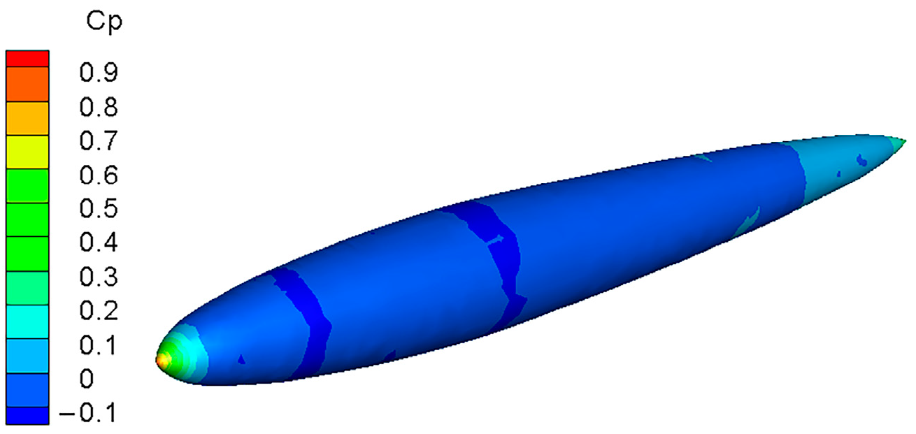
3.1. Computational Model and Boundary Conditions

This paper utilizes numerical simulation method verification based on the simplified model of the teardrop submarine “Albacore Submarine” [19]. The geometric data of this teardrop submarine model came from [20]. We used the same scaling as in reference [21], using a size scale of 1:25, model length of 3.2 m, and width of 0.4 m. The entire flow field computational domain was a cuboid, with a length 4 times the submarine length in the incoming flow direction, and 2 submarine lengths in the wake flow direction. The cross-section of the computational domain was a square with a side length 10 times the maximum width of the model. To accurately simulate the flow field flow details, $y^{+}=50$ was taken and the mesh was 127 w. The computational domain mesh is shown in Figure 1.

The boundary conditions of the flow field computational domain consist of the velocity inlet, pressure outlet, hull surface, and outer boundary. The boundary conditions were set as follows:

• Velocity inlet: The left end face (blue) of the fluid domain, with a Dirichlet boundary condition of 5 m/s velocity.
• Outflow: The right end face (yellow) of the fluid domain, located 2 submarine lengths behind the stern, so a free outflow boundary condition was used.
• Symmetry boundary condition: The upper, lower, left, and right four end faces of the fluid domain. These positions were far away from the submarine surface, so the normal velocity components on these end faces could be considered zero, thus a symmetry boundary condition was used.
• Wall boundary condition: The outer surface (green) of the model, with a no-slip boundary condition.

3.2. Computational Method

Reference [21] compared several turbulence models and concluded that better simulation accuracy could be obtained by using the RNG k-ε turbulence model. The authors did not use the LES model due to its high computer hardware requirements. In this paper, the steady flow computation used the RNG k-ε turbulence model; pressure−velocity coupling used the SIMPLE algorithm; and momentum, turbulent kinetic energy, and turbulent diffusivity used second-order upwind spatial discretization to improve the computational accuracy. After the residuals stabilized, the relevant physical variables could be observed and analyzed. With the stable steady flow results, non-steady flow calculations could begin. The LES turbulence model was chosen for the non-steady flow calculations and the FW-H acoustic model was turned on, while the export corresponded to the acoustic “CGNS” file (CGNS stands for CFD General Notation System [22]; it contains mesh data, physical variables, and storage structures in CFD calculations). The solid model material was aluminum and the fluid was water. The time step was 0.00005 s, with 1000 iterations and 50 iterations per time step to ensure convergence. The reference pressure used to calculate the sound pressure level in the water was 1 × 10⁻⁶ Pa.

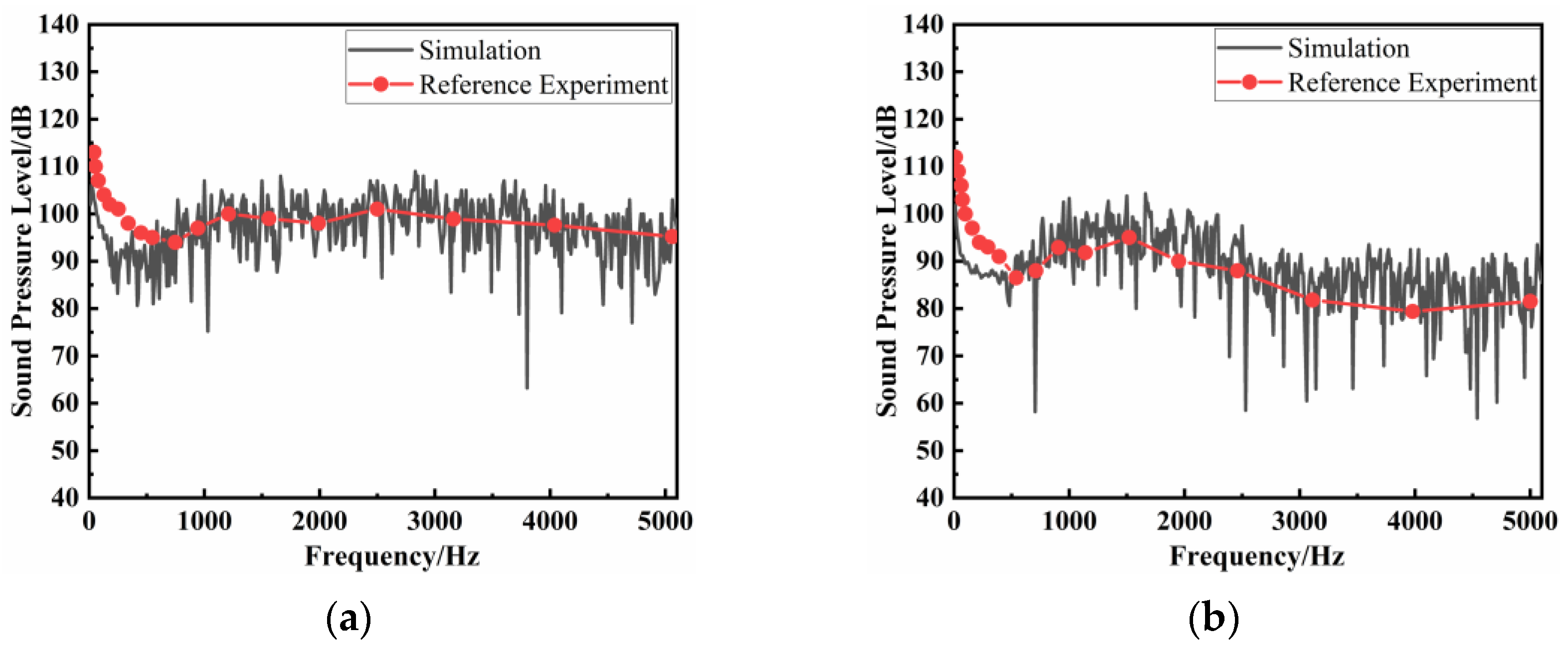
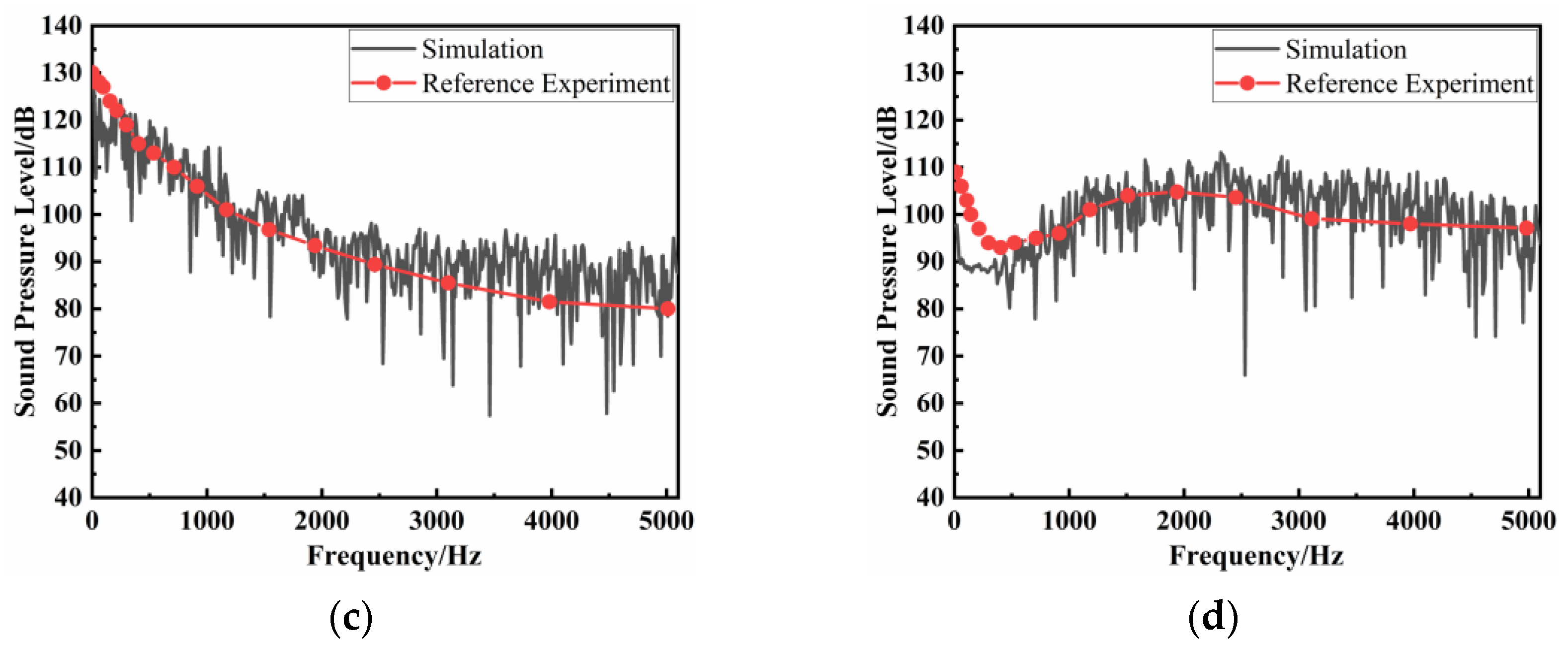
3.3. Computational Results and Analysis

The pressure coefficient distribution of the computational model is shown in Figure 2. The pressure coefficients at the front and rear ends of the model surface were large. Because the water flow collides with the submarine hull at these positions, there was a sharp decrease in fluid velocity. According to the Bernoulli equation, the pressure at these positions will increase, thus generating a higher-pressure coefficient. The velocity in the middle section was larger, so the pressure coefficient was smaller.

As shown in Figure 3, the velocity on the wall surface was zero due to the wall boundary condition. We can observe the influence of the model’s stagnation point on the velocity field, as well as the impact of the wake and trailing vortices on the flow field, which is consistent with the theory. The teardrop shape minimized shape drag to the maximum extent. Towards the rear, the streamlined design gradually narrowed, making it easier for the fluid to re-converge. This allowed water to flow more smoothly around the submarine, reducing turbulence and vortices in the water, resulting in a smaller wake. An increase in fluid velocity caused the wake to elongate and narrow. High-speed fluid would produce a longer wake, while low-speed fluid would generate a shorter wake.

Compare the numerical simulation results with the experimental data. According to the experimental data provided in reference [23], the layout of the hydrophones in the experiment is shown in

Table 1. Experimental hydrophone layout.

Hydrophone	Axial (m)	Circumferential (°)
A1	0.48	180
A2	1.28	180
A3	1.6	180
A4	2.08	180
A5	2.72	180
A6	1.6	95
A7	1.6	120
A8	1.6	150

The circumferential position refers to the angle between the hydrophone and the positive Y axis.

.

As shown in Figure 4, we compared the simulation results of hydrophones numbered 1, 3, 5, and 8 with the experimental results of the submarine’s sound pressure level.

When the frequency was less than 1000 Hz, the simulation results were slightly smaller than the experimental values, with an error of about 8%, and the variation trend was consistent with the experiment. When the frequency was greater than 1000 Hz, the simulation results were basically the same as the experimental results with the same trend. This also validated the accuracy of the numerical simulations in this study, confirming the viability of using this method for flow field calculations.

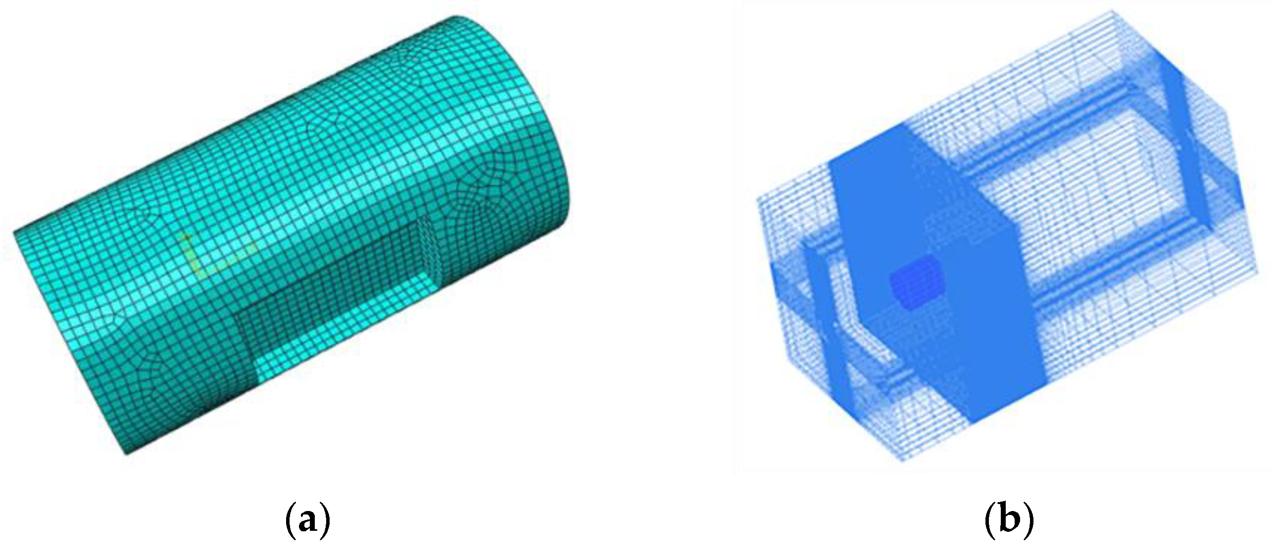
4. Noise Calculation of Cylindrical Shell Model

4.1. Computational Model

The simulation model used in this study is a simplified cylindrical shell of the experimental model. The experimental model is illustrated in Figure 5. To minimize computational resources, the experimental model underwent simplification. The hull was approximated as a cylindrical shell with a diameter of 250 mm, a length of 500 mm, and a thickness of 2 mm. Flanges with a diameter of 270 mm and a thickness of 5 mm were secured on both ends of the cylindrical shell using bolts to enclose it.

The dimensions of the flow field model for the simulation and the flow field boundary conditions were the same as those in Chapter 3. The solid model material was aluminum and the fluid was water. The flow field model mesh was generated using ICEM CFD software and the mesh was 325 w. To better obtain the flow field information and details on the shell surface, boundary layer mesh refinement was performed at the interface between the flow field and the shell. The flow field was divided into 3 blocks, with appropriate sparse mesh processing in areas not directly involved in the fluid−structure interaction. The simulation model and computational domain mesh are shown in Figure 6.

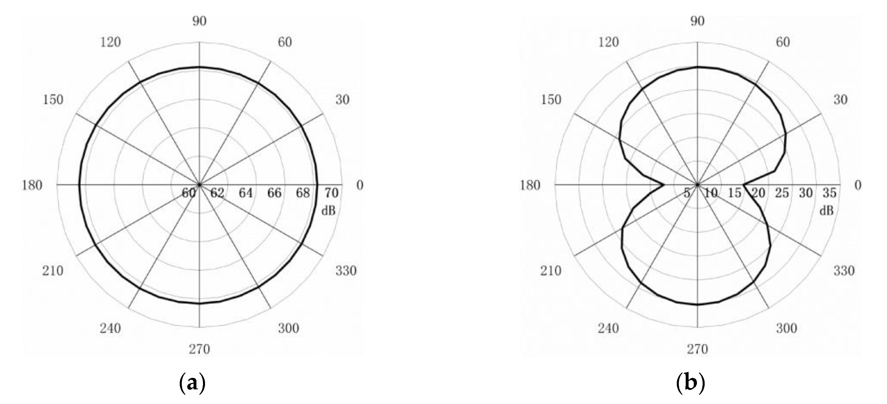
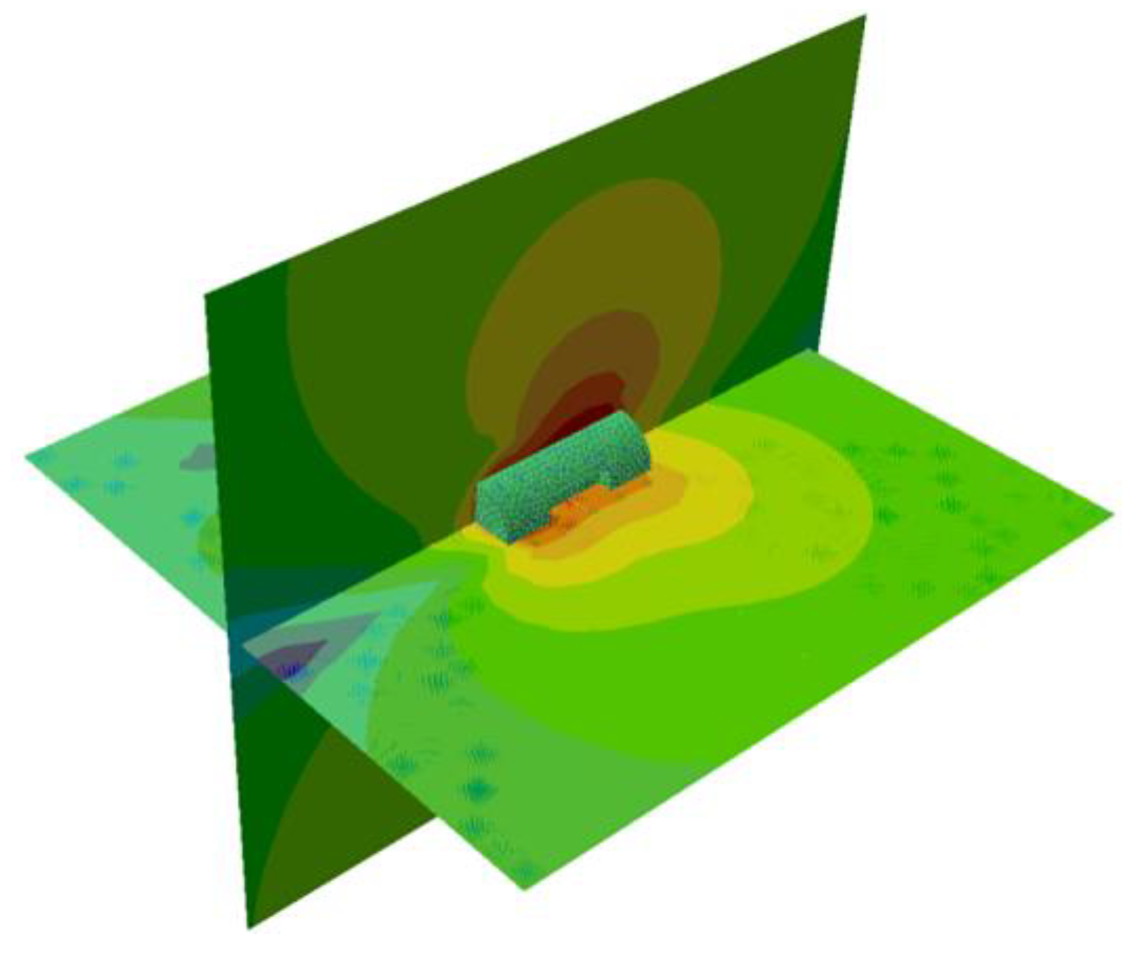
4.2. Flow Noise Calculation

The acoustic field calculation was built on the foundation of the flow field computation, and in this study, Virtual Lab acoustic simulation software was employed for the analysis. The calculated CGNS files were imported into the acoustic simulation software. The boundary element method transformed the 3D volume mesh into 2D surface integral solution by combining the Helmholtz equation with the acoustic field control equation, and acoustic analysis could be performed at any point in the acoustic field.

The acoustic directivity analysis referred to selecting points at a certain distance on the required solution surface, solving the acoustic pressure values at these points, and finally plotting the relationship between the acoustic pressure values and the angles relative to the reference axis in a polar coordinate system. This could effectively obtain the spatial distribution characteristics of flow noise.

We first analyzed the flow noise directivity of the shell. By taking the center of the shell (0, 0, 0.105 m) as the center, a circle with radius of 4 m was made on the vertical section, and an acoustic signal detection point was placed every 10° to obtain the spatial distribution characteristics of flow noise in the vertical section. Taking 2 m away from the aft shell, i.e., (0, 0, 0.355 m) as the center, a circle with radius of 4 m was made on the horizontal section, and an acoustic signal detection point was placed every 10° to obtain the spatial distribution characteristics of flow noise in the horizontal section.

From Figure 7a, it can be observed that the spatial distribution of flow noise on the vertical section was circular in shape. Because the shell was simplified as a cylinder, it had very good spatial symmetry. In the far-field, the flow noise that radiated from the shell was evenly distributed. On the horizontal section, it was difficult to directly observe the distribution characteristics of flow noise. Therefore, the flow noise values were reduced by 40 dB for observation. It can be seen from Figure 7b that the flow noise at the bow and stern decreased significantly. Because of the influence of the incoming flow and wake flow, the flow velocity at the bow and stern was lower. Hence, the noise is relatively reduced. The flow velocity in the middle part of the shell was faster, so the noise was relatively large. Because the shell structure was symmetrical on the left and right, the flow noise showed a symmetrical distribution.

4.3. Flow-Induced Noise Calculation

The calculation of flow noise regards the shell as a rigid body, but in actual situations, the shell will vibrate when subjected to surface pressure. Flow-induced noise takes structural vibrations into consideration, and it can be regarded as a composite of vibration noise generated by fluctuating pressures from the flow field and vibration-induced noise from the shell surface.

When calculating flow-induced noise, the vibration displacement of the shell surface must be considered, so fluid−structure interaction analysis is required. Because of the very small deformation in the shell structure, the volume change in the fluid domain could be neglected. So, we adopted a one-way fluid−structure interaction, considering only the influence of the fluid on the structure. The CGNS file containing flow field fluctuation information solved by Fluent was imported as the initial condition for the acoustic solution into the acoustic simulation software. The fluctuating pressure at each time step was applied as an external load to the shell structure to solve the structural dynamics equation and to obtain the displacement at each time step. Taking the derivative of displacement with respect to time could obtain the vibration velocity of the shell structure under the action of fluctuating pressure. The vibration velocities at each time node were the velocity boundary conditions when using the boundary element method to solve for flow-induced noise.

After completing the acoustic field simulation, we analyze the sound pressure nephogram at various cross-sections. The sound pressure nephogram provided us with an intuitive understanding of the spatial distribution of the acoustic field, enabling us to analyze the distribution of sound pressure at corresponding frequencies. The variations of the acoustic field around the shell are shown in Figure 8.

We conducted a comparative analysis of the longitudinal sectional sound pressure nephogram of flow-induced noise at 200 Hz, 244 Hz, 300 Hz, and 450 Hz, with results as follows:

From Figure 9, it can be observed that at frequencies of 201 Hz, 244 Hz, 302 Hz, and 450 Hz, the maximum sound pressure levels of flow-induced noise were 137 dB, 165 dB, 108 dB, and 89.2 dB, respectively. Notably, at a frequency of 244 Hz, the vibration displacement of the shell structure was significantly higher than at other frequencies. This was attributed to resonance between the shell structure and the fluid at this frequency. In comparison with other frequencies, changes in the sound pressure nephogram were observed in the near-field region. Except for 244 Hz, the sound pressure distribution near the wall was lower at the bow and stern due to the “masking effects” of the incoming flow, while the numerical values were smaller at the bow and stern than in the middle section. Overall, the sound pressure nephogram exhibited a symmetric “butterfly” pattern. As the frequency increased from 201 Hz to 302 Hz, the flow-induced noise decreased by 29 dB, and as the frequency increased from 302 Hz to 450 Hz, the flow-induced noise decreased by 19 dB. Evidently, with increasing frequency, the rate of flow-induced noise attenuation gradually decreased, and the reduction became less pronounced as the distance from the shell surface increased.

The spatial distribution characteristics of flow-induced noise are illustrated in Figure 10, with the detection points positioned in alignment with the flow noise locations.

From Figure 10, it is evident that the spatial directivity of flow-induced noise in the vertical section was consistent with that of the flow noise—both were circular in shape. It can be seen from the horizontal section that the flow-induced noise was smaller at both ends of the shell, and because there were two slots on both sides of the shell, it presented a “butterfly” shape. The sound pressure levels of flow-induced noise in horizontal and vertical sections are both greater than those of the flow noise.

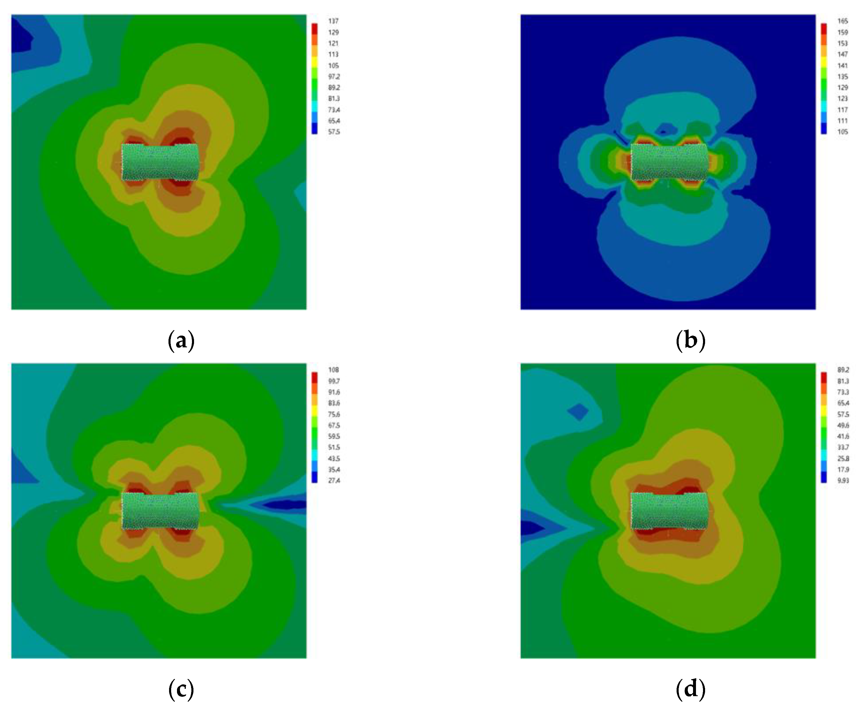
4.4. Comparison of Flow Noise and Flow-Induced Noise

The spatial distribution of the flow-induced noise can be roughly understood through the above acoustic directivity. Next, we analyzed and compared the flow-induced noise at different detection points along the X, Y, and Z axes with the flow noise.

We arranged 12 detection points along the X, Y, and Z axes, with a gradual transition from dense to sparse spacing.

Firstly, we selected detection points at both the near-field and far-field along the three axes. We conducted a comparative analysis of the spectral characteristics of flow noise and flow-induced noise, as well as the differences between the near-field and the far-field.

As shown in Figure 11, the variations in flow noise and flow-induced noise were consistent in different directions. Along the x axis, when the frequency was below 200 Hz, the flow noise and flow-induced noise were nearly equal. For frequencies above 200 Hz, both near and far-field conditions exhibited higher flow-induced noise compared with flow noise. Moreover, as the distance increased, both values gradually decreased. Beyond 400 Hz, both values tended to stabilize. It is noteworthy that at a frequency of 240 Hz, the flow-induced noise reached its maximum value, approximately 130 dB, while the corresponding flow noise levels were around 60 dB, resulting in a difference of approximately 70 dB. The noise variation trend along the y axis was similar to that along the x axis. Along the z axis, the overall noise levels were slightly lower than those along the x and y axes, but the first peak of flow-induced noise was larger. Because of the noise generated by the vibration of the shell structure, peaks in the flow-induced noise were observed at frequencies of 240 Hz, 520 Hz, and 620 Hz. These frequencies were associated with the inherent frequencies of the wet modes, indicating that resonance had a significant impact on flow-induced noise.

As shown in Figure 12, at the 12 detection points, the flow noise was consistently lower than the flow-induced noise. Along the x axis, with the increase in distance from the shell surface, the value of flow noise decreased from 117 dB to 65 dB, while the flow-induced noise decreased from 153 dB to 107 dB. The difference between the two remained around 40 dB. When the distance from the shell surface was less than 0.25 m, the reduction in flow noise was more significant than that in the flow-induced noise, and stabilized as the distance increased. For each of the detection points along the y axis, the value of flow-induced noise decreased from 150 dB to 102 dB, while the flow noise decreased from 125 dB to 57 dB, as the distance from the shell surface increased. The trend along the z axis was consistent with that of the x and y axes, with a difference of about 48 dB between the flow noise and flow-induced noise. As the distance between the detection points and the shell surface increased, flow noise decreased from 103 dB to 37 dB, while the flow-induced noise decreased from 138 dB to 80 dB, with a greater variation in flow noise. It is noteworthy that along the z axis, at the same distance, both flow noise and flow-induced noise were lower compared with the X and Y directions. This is attributed to significant variations in the flow field around the bow and stern of the shell, which reduced noise propagation.

5. Experiments

Finally, we designed towing experiments to verify the accuracy of the simulation results.

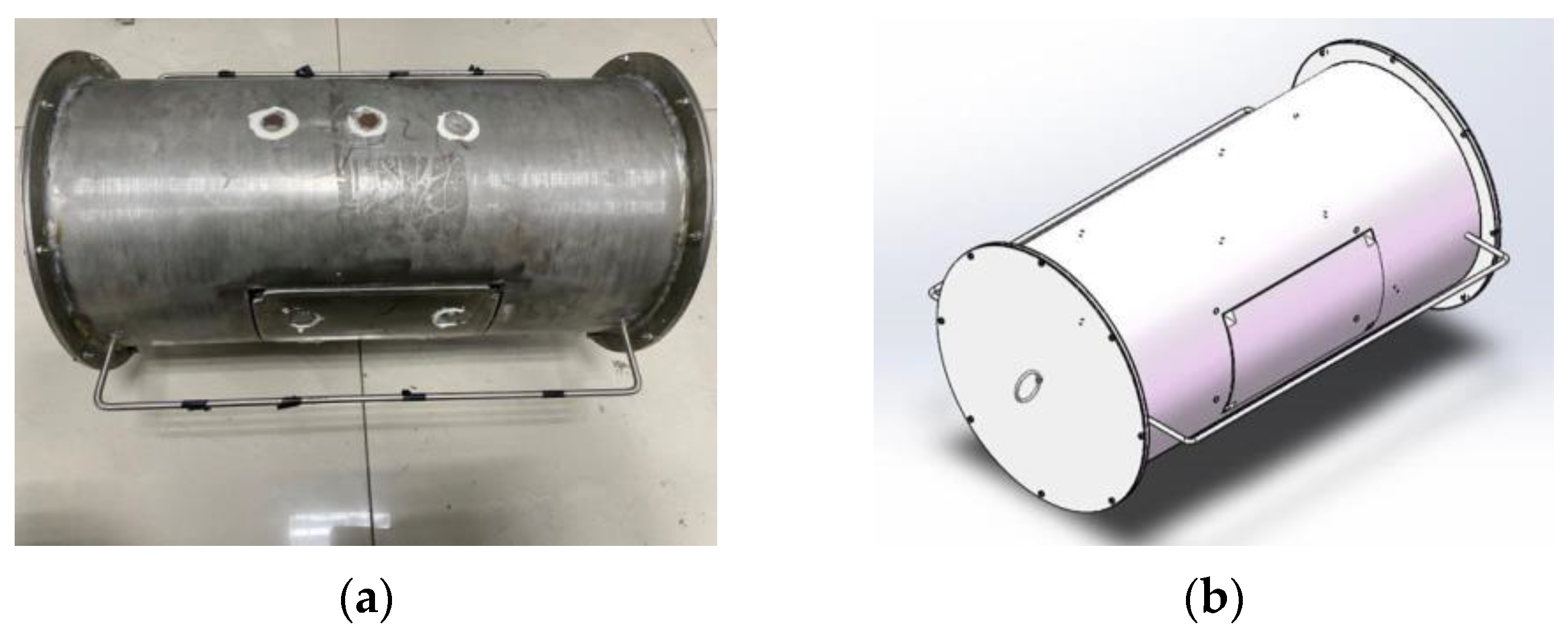
5.1. Experimental Model

The experimental model is shown in Figure 13a. Sealing rings were used at the end caps of the cylindrical shell and silicone was applied to ensure sealing of the shell. The end caps were connected to the shell body by bolts. As the cylindrical shell was hollow, the ballast body shown in Figure 13b was used for ballasting to sink the shell underwater. The ballast body was streamlined to reduce the noise generated during motion and to minimize experimental errors.

5.2. Arrangement of Experimental Instruments

As shown in Figure 14, the experimental vessel was connected to the cylindrical shell through a cable and towed by a vessel at a speed of 3 knots to capture waterborne noise signals at the vicinity of the shell. In order to ensure the stability of the underwater posture of the cylindrical shell, the ballast was placed directly under the cylindrical shell through the cable connection, and a tail rope was fixed at the tail to ensure balance.

The hydrophones were arranged on a column 40 mm away from the surface of the shell. There were 8 hydrophones in total, and the distance between them was 100 mm. The arrangement of the hydrophones on the cylindrical shell is shown in Figure 15a and the layout of the experimental detection points is shown in Figure 15b.

5.3. Signal Processing Results

The time-domain signals of each detection points acquired during the experiment underwent Fourier transform and were subsequently compared with the noise signals obtained through the simulation. This paper focuses on comparative analysis of underwater acoustic signals of detection point No. 1 and No. 4, with the results presented in Figure 16.

As shown in Figure 16, the overall variation trends in the simulation results and experimental results were basically the same. The first peak values of the two hydrophones appeared around 264 Hz and 240 Hz, with magnitudes of 110 dB and 106 dB. The first peak values in the two simulations appeared around 244 Hz, with magnitudes of 102 dB and 98 dB. The peak error was within 8%. There were certain errors between the overall simulation and experimental data, with the simulation data being smaller than the experimental data. This was because the numerical simulation was carried out under ideal conditions. In the experimental environment, environmental noise, sensor installation position, structural errors, underwater motion attitude, etc., will result in greater experimental values. Judging from the peak values in the sound pressure spectrogram, using fluid−structure coupling to solve the flow field can reflect the real underwater acoustic environment, providing experimental support for the simulation results in this study.

6. Conclusions

In this paper, we conducted research on flow noise and flow-induced noise, and validated the numerical simulation methods used. Based on this, an acoustic comparative analysis of flow noise and flow-induced noise in a cylindrical shell was performed. The following conclusions were drawn:

(1)

The validation of the computational method was performed using a teardrop submarine model, and the pressure curves at various detection points exhibited consistency with experimental trends.

(2)

According to the result of detection points at different distances in the X, Y, and Z axes, the spatial characteristics of flow noise and flow-induced noise were compared and analyzed. The results indicate that, at the same frequency, flow-induced noise was greater than flow noise. In the near-field region, both flow noise and flow-induced noise exhibited a significant decay rate, which stabilized as the distance increased.

(3)

The experimental results demonstrate that the simulated sound pressure values at the detection points exhibited a consistent trend with the experimental values, with an error of 8% at the peak. Therefore, the simulation results can effectively reflect the characteristics of the actual underwater acoustic environment.

References

1. Audoly, C. Sonar array self-noise analysis using hydrophone cross-correlation functions. J. Acoust. Soc. Am. 1995, 97, 3294. [Google Scholar] [CrossRef]
2. Cao, H.; Wen, L. High-Precision Numerical Research on Flow and Structure Noise of Underwater Vehicle. Appl. Sci. 2022, 12, 12723. [Google Scholar] [CrossRef]
3. Yu, M.; Wu, Y.; Pang, Y. A review of progress for hydrodynamic noise of ships. J. Ship Mech. 2007, 11, 152–158. [Google Scholar]
4. Liu, Y.; Li, Y.; Shang, D. The generation mechanism of the flow-induced noise from a sail hull on the scaled submarine model. Appl. Sci. 2018, 9, 106. [Google Scholar] [CrossRef]
5. Liu, Y.; Jiang, H.; Li, Y.; Shang, D. Suppression of the Hydrodynamic Noise Induced by the Horseshoe Vortex through Mechanical Vortex Generators. Appl. Sci. 2019, 9, 737. [Google Scholar] [CrossRef]
6. Lu, Y.T.; Zhang, H.X.; Pan, X.J. Numerical simulation of flow-field and flow-noise of a fully appendage submarine. J. Vib. Shock. 2008, 27, 142–146. [Google Scholar]
7. Zen, W.D.; Wang, Y.S.; Yang, Q.F. Numerical calculation of flow noise of submarine with full appendages. Acta Armamentarii 2010, 31, 1024. [Google Scholar]
8. Kellett, P.; Turan, O.; Incecik, A. A study of numerical ship underwater noise prediction. Ocean. Eng. 2013, 66, 113–120. [Google Scholar] [CrossRef]
9. Wang, C.; Deng, X.L.; Zhang, L.X. Prediction of submarine noise based on LES and infinite element method. Noise Vib. Control 2015, 35, 1–6. [Google Scholar]
10. Shi, J.D. Research on acoustic radiation characteristics of submarine current excitation based on SUBOFF mode. In Proceedings of the 17th National Academic Conference on Noise and Vibration Control, Beijing, China, 11 April 2023. [Google Scholar]
11. Jun, F.; Zhang, Z.; Wei, C.; Hong, M.; Li, J. Computational Fluid Dynamics Simulations of the Flow Field Characteristics in a Novel Exhaust Purification Muffler of Diesel Engine. J. Low Freq. Noise Vib. Act. Control 2018, 37, 816–833. [Google Scholar] [CrossRef]
12. Wahono, B.; Setiawan, A.; Lim, O. Effect of the Intake Port Flow Direction on the Stability and Characteristics of the In-Cylinder Flow Field of a Small Motorcycle Engine. Appl. Energy 2021, 288, 116659. [Google Scholar] [CrossRef]
13. Plattenburg, J.; Dreyer, J.T.; Singh, R. Vibration Control of a Cylindrical Shell with Concurrent Active Piezoelectric Patches and Passive Cardboard Liner. Mech. Syst. Signal Process. 2017, 91, 422–437. [Google Scholar] [CrossRef]
14. De Santis, D.; Shams, A. Numerical Study of Flow-Induced Vibration of Fuel Rods. Nucl. Eng. Des. 2020, 361, 110547. [Google Scholar] [CrossRef]
15. Zhu, J.; Lv, Z.; Liu, H. Thermo-Electro-Mechanical Vibration Analysis of Nonlocal Piezoelectric Nanoplates Involving Material Uncertainties. Compos. Struct. 2019, 208, 771–783. [Google Scholar] [CrossRef]
16. Lighthill, M.J. On Sound Generated Aerodynamically I. General Theory. Proc. R. Soc. Lond. Ser. A 1952, 211, 564–587. [Google Scholar]
17. Allen, M.J.; Vlahopoulos, N. Integration of finite element and boundary element methods for calculating the radiated sound from a randomly excited structure. Comput. Struct. 2000, 77, 155–169. [Google Scholar] [CrossRef]
18. Schram, C. A boundary element extension of Curle’s analogy for non-compact geometries at low-Mach numbers. J. Sound Vib. 2009, 322, 264–281. [Google Scholar] [CrossRef]
19. Shen, G.J. Submarine Design Principles, 1st ed.; Shanghai Jiao Tong University Press: Shanghai, China, 1988; pp. 14–31. [Google Scholar]
20. Moonesun, M.; Korol, Y.M. A review study on the bare hull form equations of submarine. Studies 2014, 2, 3. [Google Scholar]
21. Lu, Y.T.; Zhang, H.X.; Pan, X.J. Comparison betweenthe simulations of flow-noise of a submarine-likebody with four different turbulent models. J. Hydrodyn. 2008, 23, 348–355. [Google Scholar]
22. Legensky, S.; Edwards, D.; Bush, R.; Poirier, D.; Rumsey, C.; Cosner, R.; Towne, C. CFD general notation system (CGNS)-status and future directions. In Proceedings of the 40th AIAA Aerospace Sciences Meeting & Exhibit, Reno, NV, USA, 14–17 January 2002; p. 752. [Google Scholar]
23. Lu, Y.T. Numerical Simulation of Flow-Field and Flow-Noise of a Fully Appendage Submarine. Master’s Thesis, Shanghai Jiao Tong University, Shanghai, China, 2008. [Google Scholar]
Figure 1. Mesh of the computational domain.
Applsci 13 11095 g001
Figure 2. Pressure coefficient distribution of the computational model.
Applsci 13 11095 g002
Figure 3. Cross-sectional velocity distribution of the computational model.
Applsci 13 11095 g003
Figure 4. Sound pressure level comparison: (a) no. 1; (b) no. 3; (c) no. 5; (d) no. 8.
Applsci 13 11095 g004aApplsci 13 11095 g004b
Figure 5. Experimental and simulation models: (a) experimental model and (b) simulation model.
Applsci 13 11095 g005
Figure 6. Simulation model and computational domain mesh: (a) simulation model mesh and (b) computational domain mesh.
Applsci 13 11095 g006
Figure 7. Flow noise acoustic directivity diagram: (a) vertical section and (b) horizontal section.
Applsci 13 11095 g007
Figure 8. Acoustic field around the shell.
Applsci 13 11095 g008
Figure 9. Flow-induced noise sound pressure nephogram: (a) 201 Hz; (b) 244 Hz; (c) 302 Hz; (d) 450 Hz.
Applsci 13 11095 g009
Figure 10. Flow-induced noise acoustic directivity diagram: (a) vertical section; (b) horizontal section.
Applsci 13 11095 g010
Figure 11. Noise comparison diagram: (a) detection point X1; (b) detection point X11; (c) detection point Y1; (d) detection point Y11; (e) detection point Z1; (f) detection point Z11.
Applsci 13 11095 g011
Figure 12. Comparison of sound pressure level: (a) X axis; (b) Y axis; (c) Z axis.
Applsci 13 11095 g012
Figure 13. Experimental model: (a) cylindrical shell and (b) ballast body.
Applsci 13 11095 g013
Figure 14. Schematic diagram of the experimental dragging.
Applsci 13 11095 g014
Figure 15. Experimental arrangement: (a) experiment equipment; (b) schematic diagram of detection point layout. #1–#8 in (b) represent the location of the hydrophone detection points.
Applsci 13 11095 g015
Figure 16. Frequency spectrum diagram: (a) no. 1 detection point; (b) no. 4 detection point.
Applsci 13 11095 g016