Abstract
Rotary shaft seals prevent the exchange of fluid at shaft passages. Their function and service life depend decisively on the temperature in the contact area between the sealing edge and the shaft. Since the temperature depends on both the generation of frictional heat in the contact area and the heat transfer to the surrounding sealing system, the design of the sealing system is crucial. Within the scope of this work, multiphase conjugate heat-transfer analyses were performed considering different assembly situations. The computed results were presented and contrasted to experimental data. This resulted in a valid model for predicting the temperature in the sealing system, which provided insight into the influence of the sealing surroundings on the contact temperature.
1. Introduction
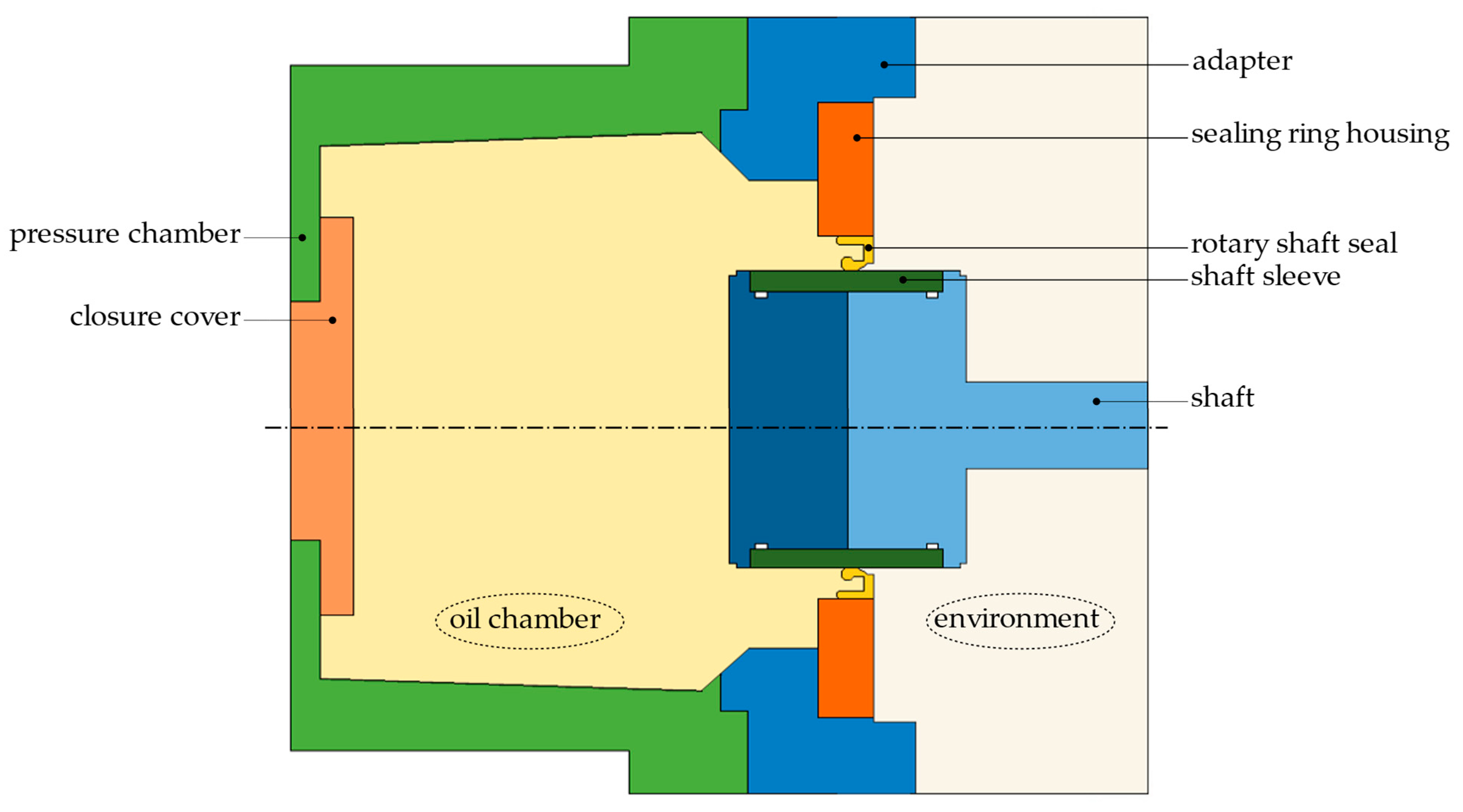
In many technical applications, seals are required to keep lubricants and operating fluids within a system as well as to keep contaminants out of this system. Rotary shaft seals (RSS) are mainly used to seal pressureless shaft passages that are splashed or flooded, e.g., in automotive and mechanical engineering [1,2]. The rotary shaft seal is a complex tribological system that includes not only the sealing ring, but also its counterface, i.e., the shaft surface, and the fluid to be sealed [1]. The sectional view of a rotary shaft seal made of elastomer according to DIN 3760 [3] or ISO 6194 [2] is shown in Figure 1.
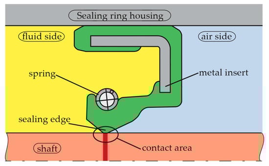
Figure 1.
Sectional view of a rotary shaft sealing ring made of elastomer.
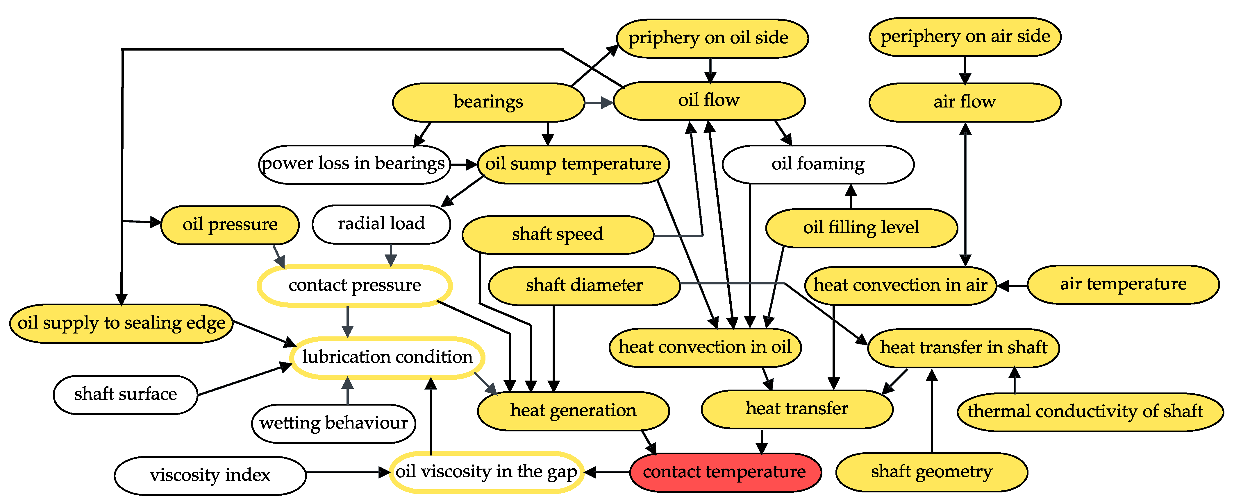
In the assembled state, the sealing lip is pressed against the shaft surface with the aid of a garter spring. This results in a narrow contact area between the sealing edge and the shaft surface, with a contact width of about 0.1 mm [1]. The static sealing mechanism, i.e., when the shaft is not rotating, is additionally ensured by the interference of the shaft outer diameter and the sealing ring inner diameter [1]. When the shaft rotates, the lubricant to be sealed is dragged into the contact area between the sealing edge and the shaft. Due to the active sealing mechanism, this fluid entering the sealing gap is pumped back from the air side to the oil side. Various models have been suggested to explain this dynamic sealing mechanism of rotary shaft seals [4,5,6]. During operation, the contact area is subjected to friction. The more frictional heat is generated in the contact area and the less of this heat can be dissipated from the contact area, the greater the temperature in the contact area. The generation and dissipation of heat and, thus, the contact temperature is affected by numerous interacting factors, some of which are illustrated in Figure 2.
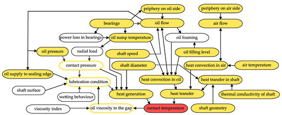
Figure 2.
Factors affecting the contact temperature, according to [7].
Failures of rotary shaft seals and, thus, of the entire system are often caused by the overheating of the contact area. An increase in temperature in the sealing contact of about 10 K can already lead to a significantly reduced service life of a rotary shaft seal [8]. Therefore, in order to better assess the risk of a temperature-induced failure and to achieve a long service life, the temperatures in the contact area must be below the operating temperature limit of the sealing ring and the fluid. The contact temperature to be expected during operation must, thus, be known as accurately as possible. In general, it can be distinguished between three different ways of determining the contact temperature. The first option is to measure directly on a real component [9]. This is usually the most accurate method for determining the contact temperature, but these measurements can be extremely difficult or even impossible due to the very small gap heights between the sealing edge and the shaft. Furthermore, a prototype must already have been manufactured. For an initial design, before a prototype is manufactured, these measurements, therefore, cannot be performed. The second option is the possibility of estimating the temperature in the contact area without a prototype by using an approximation equation [7,10,11]. This can be conducted, for example, with the InsECT beta-18.10.08 [12,13] calculation tool developed at the Institute of Machine Components of the University of Stuttgart. In the current state of development, this tool is not applicable to sealing systems with certain configurations, such as rotary shaft seals with a protective lip or coated shafts, hollow shafts or shafts with sleeves. The third option is to simulate the entire system. Through simulations, the expected contact temperature can already be developed for the first design without the need to build a prototype. This offers the possibility to simulate different variants and compare them with each other. Moreover, the results are more accurate than when using approximation equations. Depending on the complexity of the simulation model, i.e., how many influencing factors are considered, the development of the simulation model can be extensive and, thus, require a great amount of time.
As the shaft rotates, the sealing edge lifts up, resulting in the formation of a thin lubricating film in the sealing gap. Thus, there is no fixed boundary between the fluid to be sealed, the oil, and the surrounding fluid, the air. For the prediction of, for example, cavitation zones in the sealing gap, this multiphase flow has already been successfully simulated in the past [14,15]. Finite element analysis (FEA) of a rotary shaft seal has already been used to analyze the radial deformation and contact pressure distribution [16,17,18]. In addition, elastohydrodynamic lubrication (EHL) simulations have also been performed [19]. In general, the focus of the EHL simulations was mainly the investigation of the flow in the sealing gap [15]. By focusing on the lubricant film in the sealing gap, many of the influencing factors, shown in Figure 2, could not be considered. A simulation of the whole test bench, as it was performed in this work, has been performed in the past [20]. However, the focus was not on the design of the surroundings of the sealing ring either. Therefore, it has not yet been possible to predict what impact the surroundings of the sealing ring have on the contact temperature. The work described in this paper is intended to enable an understanding of the influence of the sealing surroundings on the contact temperature.
In this study, the temperature in the contact area between the sealing edge and shaft was determined for different geometric variants by measurements on the test bench and additionally by simulations. An only-slightly simplified geometry of the test bench was used for the simulations. Since the development of different simulation models is time-consuming and, therefore, it is usually not possible to develop many different models within the given time, parameterized simulation models were used. The interacting factors, highlighted with a yellow background in Figure 2, were all considered in the simulations. The factors indicated by a yellow frame were included only partially, e.g., as a boundary condition. As far as possible, we tried to reproduce reality in the simulations. However, due to limited computing power, some simplifications had to be made. The temperatures in the contact area resulting from the simulations were compared with the temperatures measured in the experiments on the test bench. In this way, it was possible to evaluate which of the simplifications made still led to accurate simulation results.
2. Materials and Methods
A total of 17 different simulations were performed in the computational-fluid-dynamics (CFD) software Ansys CFX 2021 R2. One reference configuration and 16 geometric variations were used. Due to the heat transfer between the solid domains and fluid domains in the model, the conjugate heat-transfer (CHT) method was used. This method calculates the temperature distributions in both the fluids and the solids. The flow in the sealing gap was neglected. Due to the interaction between the oil and air in the oil chamber, a multiphase flow was considered. To validate the results obtained from the simulations, experiments were performed on a test bench at the institute.
2.1. Governing Equations
The convective heat transfer in the fluids around the sealing system was described using the Navier–Stokes equations in their conservation form. The heat conduction in the solids of the sealing system and its surroundings was described with the help of the energy equation. Therefore, the following conservation equations of mass, momentum and energy had to be satisfied.
The continuity equation
with the flow velocity vector field U, the time t and the fluid density describe the conservation of mass. This equation ensures that the mass entering a system is equal to the mass leaving the system and the accumulation of mass within the system. The first part, the time derivative, describes the loss of mass in the system and the second part, the divergence term, describes the difference between the mass entering and the mass leaving the system. Since the air is assumed to be incompressible, the density is constant and the continuity equation can be simplified to [21]:
The momentum equation
where the shear-stress tensor for Newtonian fluids and the pressure are an expression of Newton’s second law of motion and describes the conservation of momentum for moving fluid [22]. The optional source terms depend on the application. For example, if buoyancy is considered, the source term
is added to the momentum equations, where = 9.81 m/s2 is the gravitational acceleration [23].
The total energy equation is
where the thermal conductivity is and the total enthalpy is
This states that the total energy of the system is equal to the total work and heat added to the system. The viscous work term represents the work due to viscous stresses, and the term describes the work due to an external momentum source. The volumetric heat source is optional [23].
In addition to the conservation equations, equations for the determination of the heat transfer must be solved. Heat transfer refers to all processes of transporting energy in the form of heat. The “internal energy”, i.e., the energy contained in a system, is a state variable. In addition, the energy exists as a conservation variable, as it cannot be created or destroyed, but transformed into another form. This is described by the first law of thermodynamics:
where describes the heat flow across the system boundary and the working current across the system boundary. For a stationary system, the mass flow is equal to the incoming mass flow and equal to the outgoing mass flow. The specific enthalpy is divided into the incoming enthalpy and outgoing enthalpy . As two systems of different temperatures come into contact with each other, heat is exchanged along the negative temperature gradient. The first law of thermodynamics described in Equation (7) does not affect how heat is transferred between multiple systems. Heat can be transferred by conduction, convection or radiation. Thermal radiation is neglected in this work.
When several systems do not move relative to each other, have different temperatures and are in contact with each other via their surfaces, heat conduction occurs [24]. During heat conduction, no mass is transferred; the heat exchange takes place due to atomic interactions. Fourier’s law,
describes the heat-flux density transported by heat conduction within the same phase [21]. The heat flux in Equation (7) is defined as the amount of thermal energy leaving/entering the system in a given time across the system boundary. The heat-flux density is defined as the amount of thermal energy leaving/entering within a certain time, but related to a cross-section .
The convective heat transfer is the transfer of heat between a solid and a moving fluid or between two fluids [24]. The amount of heat transferred is strongly dependent on the fluid layer close to the wall, the so-called boundary layer. In this boundary layer, the temperature changes from the wall temperature to the temperature of the fluid within a short distance. In addition, the velocity of the fluid increases from the value zero at the wall to the mean fluid velocity. Since the temperature and velocity profile in the boundary layer are usually unknown, the heat transfer coefficient is introduced. Using this heat transfer coefficient, the heat flux density can be calculated by
In the solid domains, the equation for the heat transfer is solved without any flow. Within these domains, the equation for the conservation of energy, Equation (5), can be modified to
To model the two-phase flow in a domain containing air and oil, the VOF (volume of fluid) model with completely homogeneous equations for two fluids was used. The free-surface model was used for the interface description. In the VOF model, the volume fraction of a phase within a calculation cell is stored as an additional variable . This variable is transported convectively with the velocity through the domain, which is described by the transport equation:
where for a two-phase domain with air and oil [25,26]. The constraint
has to be fulfilled in each calculation cell. In the cells that contain both fluids, the properties are calculated using a volume fraction average of the fluids. Thus, for example the density in a cell, can be described by
These averaged properties are then used to solve the momentum equation stated in Equation (3).
2.2. Modeling
In the following, the setup of the 3-dimensional simulation model in the Ansys CFX 2021 R2 software is explained. This includes the computational domain, the computational grid, the definition of the material parameters and boundary conditions, and the solver settings.
2.2.1. Computational Domain
The tests used to validate the simulation model were performed on a high-speed friction torque test bench. The rotationally symmetrical geometry model used in the simulations was based on this test bench and consisted of a total of nine domains, which are illustrated in Figure 3. The domains pressure chamber, closure cover, adapter, sealing ring housing, rotary shaft seal, shaft sleeve and shaft were considered as solid bodies. The geometry of the sealing ring used on the test bench was simplified in the simulations: neither the spring nor the metal insert of the sealing ring were considered, and the entire volume of the sealing ring was assumed to be made of elastomer. Both the sealing edge and the shaft as the counterface were assumed to be ideally smooth. The sealing gap itself was not simulated, but the direct contact of the sealing edge to the shaft was assumed. The fluid domain oil chamber contained both oil and air, which is why a multiphase model was necessary to describe the two-phase flow. The fluid domain environment contained only the air.

Figure 3.
Geometry of the reference variant: A sectional view of the 3-dimensional model.
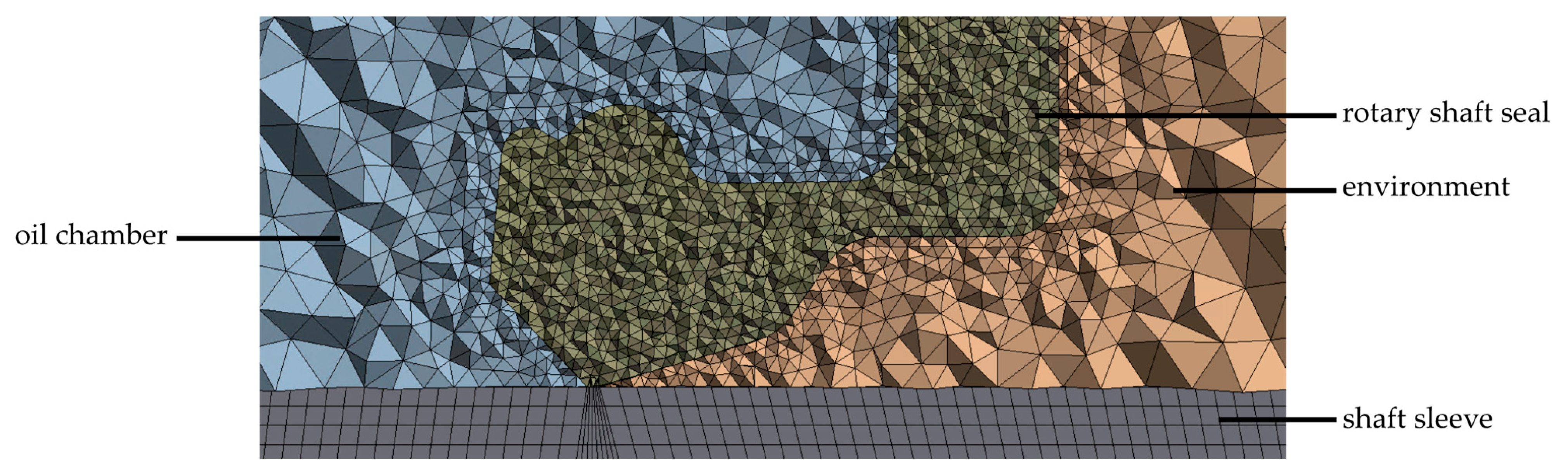
The geometry was meshed in the Ansys Workbench meshing software, Ansys CFX 2021 R2. An element size was specified for each domain. The sealing ring was meshed with the finest element size of 0.2 mm. To ensure a smooth transition to the surrounding domains and, thus, to other element sizes, the mesh size at the interfaces of the sealing ring was also set to 0.2 mm. Over the 0.2 mm wide contact width between the sealing edge and the shaft sleeve, the number of elements was set to 8 elements. The domains environment and oil chamber were meshed with an element size of 1 mm. The largest mesh size of 4 mm was defined for the domains pressure chamber, adapter and closure cover. The used mesh contained 60.5 million elements and 13.7 million nodes. Due to the limited computing power available, the mesh was not further refined. Figure 4 shows the mesh in the area of the sealing edge. The domains rotary shaft seal, oil chamber and environment were meshed with tetrahedrons; all other domains were meshed with hexahedrons.
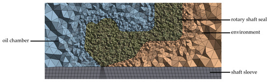
Figure 4.
Mesh in the area of the sealing edge: Sectional view of the 3-dimensional model.
2.2.2. Material Data
A total of three solid materials were defined: elastomer, aluminum and steel. For each of these materials, the density, specific heat capacity and thermal conductivity were defined. The material data used are listed in Table 1. The values given in the table are constant material parameters, independent of temperature and pressure. Only the density and thermal conductivity of the air (ideal gas), as well as the dynamic viscosity of the oil, were assumed to be non-constant. The constant material data were defined as expressions. This way of parameterizing the simulation model allowed the individual parameters to be changed easily and in a fast way. Rotary shaft seals from Freudenberg made of the fluororubber compound 75FKM585 [27] were used for the experiments on the test bench. The material data of the elastomer used in the simulations were based on this fluororubber compound. As material data of the steel, the data of the steel 100Cr6 [28] were used, since this steel was used in the experiments. The aluminum was the aluminum–copper alloy EN AW 2007. The fluid domain environment was filled with air (ideal gas). The default values of Ansys were used as material data of the air. The fluid domain oil chamber was filled with oil up to a defined oil fill level; everything above this level was initially assumed to be air (ideal gas). The oil Fuchs Titan Supersyn Longlife 0W-30 was used for the experiments. The density of the oil was measured with a pycnometer according to EN ISO 3838 [29]. The values of the specific heat capacity and the thermal conductivity of the oil were estimated based on experiments [30] and other oils [31].

Table 1.
Material data of the solid and fluid materials used in the simulation.
Since the density of air is affected by the current temperature and the pressure , the air density was not assumed to be constant and was defined as
where is the molar mass of the air and is the universal gas constant. Below the boiling point, the thermal conductivity of gases increases linearly with temperature, allowing a 1st-degree polynomial to be sufficient to correlate measured values [24]. The thermal-conductivity data of dry air at 20 °C and 120 °C from [24] was used to define the thermal conductivity of air as
as a function of the current air temperature . Since no temperature-dependent data of the thermal conductivity of the oil were available, the conductivity of the oil was assumed to be constant.
The dynamic viscosity of the air was defined as kg/(m·s). To describe the temperature-dependent viscosity of the oil, the Vogel equation
with the temperature-independent material parameters and and the Vogel temperature was used [32,33]. To determine these parameters, measurements with a MCR302 rheometer manufactured by Anton Paar Germany GmbH (Ostfildern, Germany) were made. Both the dynamic viscosity of the air and the dynamic viscosity of the oil were defined as expressions.
2.2.3. Boundary and Initial Conditions
The shaft and shaft sleeve were defined as rotating. The rotational speed was specified as an expression and could, thus, be easily varied. All other solid domains were stationary. Due to the rotation of the shaft sleeve, frictional heat was generated in the contact area between the shaft sleeve and the sealing ring. The frictional heat model
describes the frictional heat flux generated in the contact area [7]. This frictional heat flux was introduced to the simulation model via a boundary condition. Therefore, the frictional torque was measured on the test bench for different shaft speeds and approximated by the rational function
according to [15]. The measured values were then fitted to the curve described by Equation (18) in order to determine the parameters , , and . With the help of this fitted curve, the values of the frictional torque can then be approximated for various shaft speeds, which may not have been measured. The parameters in Equation (18) were only valid for the tribological system with which the measurements were performed. For other materials or different geometries, the parameters had to be redetermined.
In reality, the heat calculated by Equation (17) is generated in the sealing gap between the sealing ring and the shaft surface. Since the thermal conductivity of the sealing ring is extremely low compared to the thermal conductivity of the shaft, more heat is transferred from the sealing gap to the shaft than to the sealing ring. In the simulation model, the sealing gap was not considered; instead, the direct contact between the shaft surface and the sealing edge was assumed. In order to realize the uneven heat transfer to the sealing ring and the shaft in the simulation model, the frictional heat flux calculated by Equation (17) was divided into two parts. A larger part of the heat flux was specified as a heat source at the shaft surface. A much smaller heat source was specified at the sealing edge. Thus, the frictional heat flux determined by Equation (17) was divided using a heat partition factor which is defined as
By inserting the frictional torque into Equation (17) and then multiplying the resulting frictional heat flux with the heat partition factor, the frictional heat applied to the sealing ring could be determined by
and the frictional heat applied to the shaft sleeve analogously by
The frictional heat of the shaft was added as a heat source in the contact area between the shaft sleeve and sealing ring, but only to the shaft sleeve. The frictional heat of the sealing ring was also added in the contact area, but only on the side of the sealing ring.
Except for the fluid domain environment, each domain was initialized with the initial temperature = 80 °C. This corresponds to the oil sump temperature at the test bench, to which the oil was heated during the experiments. The domain environment was initialized with the ambient temperature = 20 °C. For the boundary condition on the outer side of the domains pressure chamber and adapter/bearing housing, the heat transfer coefficient = 42.5 W/(m·K) was specified as the boundary transition to the ambient temperature . A subsonic opening boundary condition was defined at the system boundary of the domain environment. Thus, the fluid in this domain, the air, was allowed to cross the boundary surface in either direction. The flow over the boundary did not have to be normal to the surface. The static pressure was specified as 0 Pa over this boundary. To represent the holder of the spindle and, thus, a wall, the axial system boundary of the domain environment was defined as a no-slip wall. This meant that the velocity of the air at this boundary was set to zero. Due to the adiabatic option, this wall allowed no heat transfer across the wall boundary.
At high Reynolds numbers, when the inertial forces in the fluid become much larger than the viscous forces, turbulence occurs [23]. For this reason, a turbulence model was used in the domain oil chamber. This allowed the effect of turbulence to be considered without having to use an extremely fine mesh or direct numerical simulations. An Eddy Viscosity Turbulence Model, Menter’s two-equation Shear Stress Transport model of [34,35] was used to model the turbulence. It was assumed that the turbulence in the model consisted of small vortices, which built up and dissipated continuously [36]. This turbulence model provided good computational accuracy with a relatively low numerical effort, and has been used successfully in the past [20].
2.2.4. Solver Settings
The advection scheme “High resolutions” was used. This defines how the advection term in the transport equation is modeled numerically. The “High resolution” scheme keeps the solution as close to the second order as possible. To under-relax the equations of the steady-state simulation as they iterated towards the final solution, a false time step was applied [37]. As a fluid timescale control, the option “Auto timescale” was defined. With this option, the solver calculates the timescale based on the defined boundary conditions, initial conditions or the current solution. The same option was used for the solid timescale. This automatically calculates the solid time scale based on the length scale, thermal conductivity, density and specific heat capacity. The timescale in the solid domains, without any flow, was defined separately, because these timescales can usually be much longer.
The convergence criteria define when a solution is considered converged and, thus, when the solver will stop. The maximum residual (root mean square) was set to 0.0001. The maximum number of outer loop iterations was set to 100. Thus, the solver terminated after 100 iterations, regardless of whether the specified convergence criterion was reached or not. By monitoring the residual and different temperatures per monitor points, it was confirmed that this limit was sufficient.
2.3. Case Studies
In addition to the reference configuration explained in Section 2.2, 16 other configurations were simulated. All 16 variants could be divided into the two subgroups variants with additional elements and variants of the shaft design. In total, only two simulation models, one for each subgroup, had to be created. Due to the possibility of defining various parameters in the simulation software, new variants could be simulated quickly and without great effort. Thus, all these variants could not only be tested on the test bench, but also simulated for different shaft speeds.
2.3.1. Variants with Additional Elements
To protect the sealing edge from penetrating liquids or contamination, an additional slinger disc can be installed. Baffle plates are used to intercept and control large volumes of oil or dirt and thereby prevent damage to the sealing lip. Studies by Kunstfeld [38] have shown that components surrounding the sealing system, for example, bearings, slinger discs or baffle plates, have an influence on the temperature in the sealing contact. Therefore, different combinations with additional elements close to the sealing edge were simulated. These configurations with additional elements are listed in Table 2.
Table 2.
Simulated variants with additional elements.
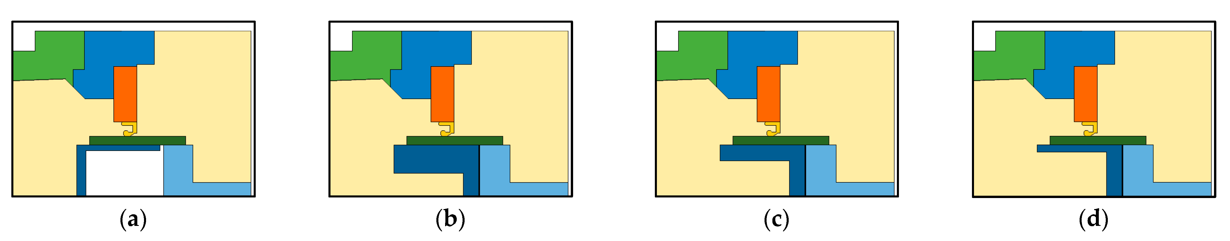
The computer-aided designs (CAD) of the first four variants in Table 2 are shown in Figure 5. For the variants with a baffle plate, seen in Figure 5c,d, the volume between the baffle plate and the cover was not considered in the simulations. The boundaries to this volume are adiabat. Two different arrangements of tapered roller bearings, the X-arrangement and the O-arrangement, ball bearings and cylindrical roller bearings were tested on the test bench. The sectional views of the geometries of the four-bearing arrangements are shown in Figure 6. The diameter of the bearings was the same for all four.
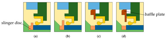
Figure 5.
Simulated configurations with slinger disc and baffle plate. (a) SD_small. (b) SD_large. (c) BP_small. (d) BP_large.
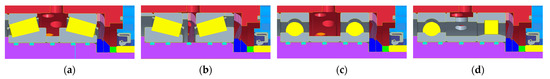
Figure 6.
Geometry of the bearing arrangements. (a) X-arrangement. (b) O-arrangement. (c) ball bearing. (d) cylindrical roller.
The maximum temperatures, which are the main focus of the simulation, were found in the contact area between the sealing ring and the shaft. Due to the distance to the contact area, the geometry of the bearings was assumed to have no great influence on the contact temperature. Thus, to keep the simulation setup as simple as possible, the same geometry model was used for the simulations of the four variants with bearings, as shown in Figure 7.
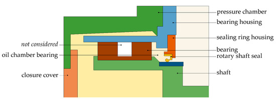
Figure 7.
Sectional view of the 3-dimensional simulation model for the variants with bearings.
Different pumping effects could be observed for different bearings. In the case of the tapered roller bearings, the fluid was pumped towards the larger diameter of the taper [39]. In the X-arrangement, the fluid located between the sealing ring and the bearings was pumped away from the sealing ring. In the O-arrangement, the fluid was pumped towards the sealing ring. For the variants with bearings, there were two fluid domains filled with oil and air: the domain oil chamber and the domain oil chamber bearing. Depending on the bearing and its pumping effect, a different amount of oil reached the domain oil chamber bearing. Thus, the only differences between the variants with bearings were the following:
- The oil fill level in the domain oil chamber bearing;
- The frictional torque between the bearing and the shaft.
The fluid domain oil chamber bearing was filled with oil up to the oil fill level ; everything above this level was initially assumed to be air.
2.3.2. Variants of the Shaft Design
The shaft was modeled as the following:
- An air-filled hollow shaft, illustrated in Figure 8a;
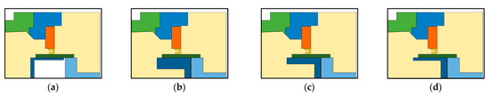 Figure 8. Simulated configurations, hollow shaft designs. (a) air_filled. (b) oil_filled_35. (c) oil_filled_50. (d) oil_filled_60.
 - An oil-filled hollow shaft, illustrated in Figure 8b–d;
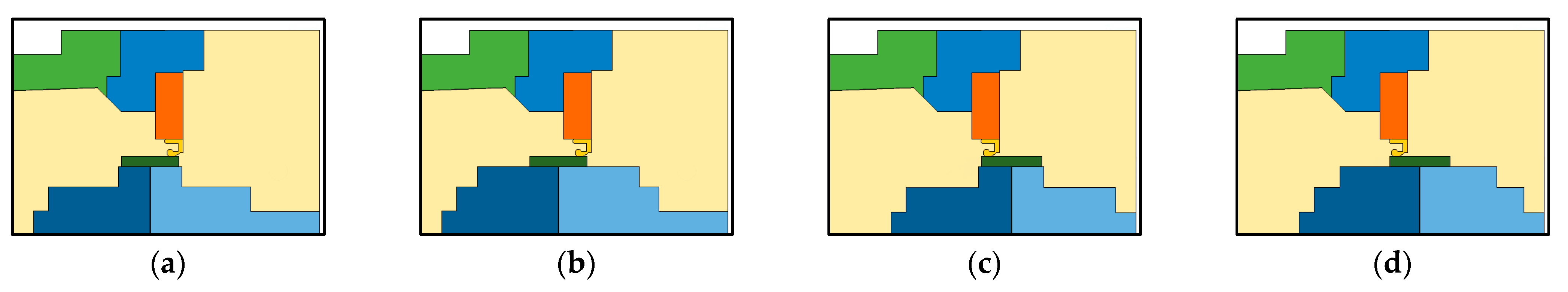
- A solid shaft with various shaft shoulders, illustrated in Figure 9.
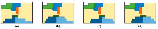 Figure 9. Simulated configurations: shaft shoulder designs. (a) shoulder_air_short. (b) shoulder_air_long. (c) shoulder_oil_short. (d) shoulder_oil_long.
The simulated combinations with these additional elements are listed in Table 3.
Table 3.
Simulated variants of the shaft design.
The four variants with a hollow shaft differ in the fluid inside the shaft and in the inner diameter of shaft, as seen in Figure 8. The inside of the air-filled shaft was not considered in the simulation model, and the boundaries to this volume were assumed to be adiabat.
Two different geometries were used for the variants with shoulders, one with a wide shaft, i.e., with a long shoulder, and one with a narrow shaft, i.e., with a short shoulder. The shaft sleeve was simulated on two different positions for each shoulder width and was either on the air-side or on the oil-side of the sealing ring, as shown in Figure 9.
2.4. Experiments
The high-speed friction torque test bench shown in Figure 10 was used for the experiments [30]. The basic design of the test bench consists of a spindle driven by a motor, on which the shaft is mounted, and an aerostatic bearing into which the test chamber is mounted. The motor can realize speeds of up to 24,000 rev/min. The entire test chamber can be moved along linear guides. By adjusting the trapezoidal spindle, different positions of the shaft can be set, for example to test the variants with shoulder design. The aerostatic bearing allows the chamber to rotate around the center axis with minimal friction, which is required to prevent the measurement of a falsified frictional torque. The chamber is supported by a lever arm acting on a load cell. The friction generated at the seal is, thus, passed on to the chamber and measured via the load cell. Before starting the test, the oil chamber was filled with oil up to the center of the shaft and then closed with a vent valve. The temperature of the oil inside the oil chamber was monitored with a temperature sensor PT 100. The test-bench control regulated heating cartridges to keep the oil temperature at the desired temperature. For the experiments in the scope of this study, the temperature of the oil was heated to = 80 °C. In order to obtain measurement results at different shaft speeds, a speed duty cycle, in which the speed was increased in predefined steps, was run after a twelve-hour run-in phase. Both the frictional torque and the temperature in the contact area were measured at each speed level in the last few minutes of a 30 min speed step in the speed duty cycle.
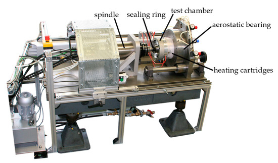
Figure 10.
High-speed friction torque test bench.
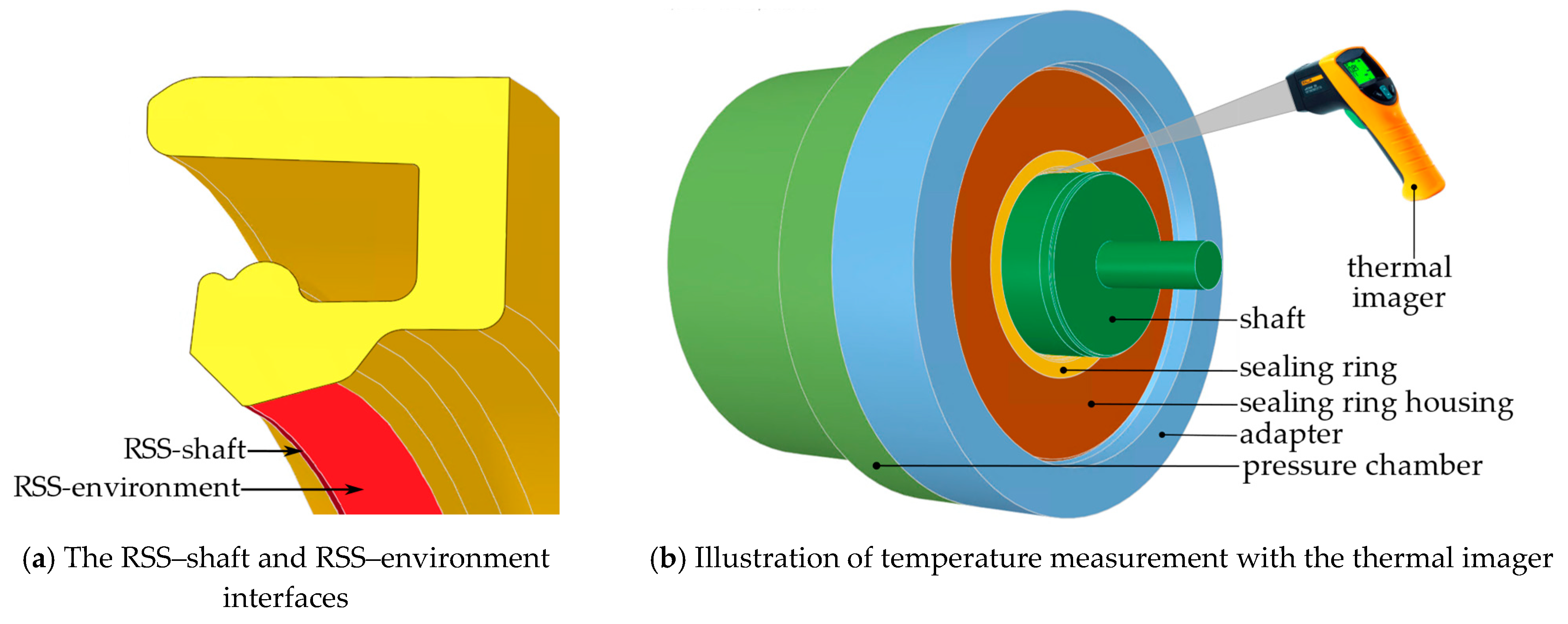
A thermal imager (Ti480 PRO from Fluke) was used to measure the temperature near the air-side contact surface of the sealing edge with the shaft. All objects emit an electromagnetic radiation depending on their temperature; the hotter, the more intense. With the thermographic camera, the intensity of this radiation can be observed in the infrared range. The intensity of this radiation depends on the surface condition of the measured object or its emissivity. This influencing factor was set beforehand by calibrating the device. An emission coefficient of ε = 0.95, a transmissivity of 100%, and a background temperature of 22 °C were set for all measurements. The maximum temperature displayed on the thermographic camera was used as the measured value.
3. Results
In the following, the oil distribution in the oil chamber and the initial condition of the oil are shown first. The temperature distribution in the cross-section resulting from the simulation for different rotational shaft speeds is shown next. The simulations were performed on a workstation with an Intel Xeon W-2155 (Intel, Neubiberg, Germany) with a clock speed of 3.30 GHz and 128 GB of RAM. When running on 10 cores, the simulation finished 100 iterations, which was the maximum number of iterations due to the predefined solver settings, after about 40 min.
3.1. Phase Interaction
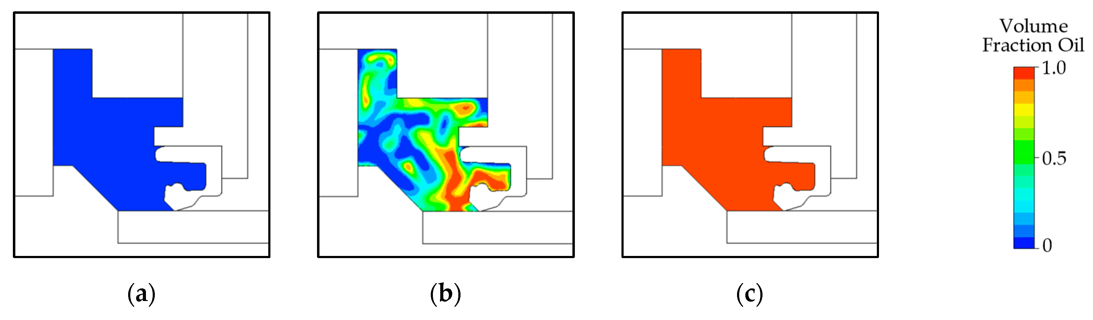
For different rotational shaft speeds , the frictional torque and, thus, the heat source in the sealing contact changed, as demonstrated by Equation (17). The higher the shaft speed, the more heat was generated. In addition, the distribution of the oil in the oil chamber changed for different shaft speeds, as shown in Figure 11. The higher the speed, the more oil was dragged against the outer wall of the oil chamber. This has been confirmed by observations from various tests [40].
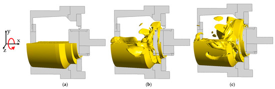
Figure 11.
Oil distribution in the oil chamber for different rotational shaft speeds, reference variant. (a) = 0 rev/min. (b) = 2000 rev/min. (c) = 8000 rev/min.
Initially, the oil in the oil chamber was assumed to be everywhere below the height of the center of the shaft, as shown in Figure 11a. Due to the rotating shaft and the resulting centrifugal force, the oil was distributed in the oil chamber. In addition, the gravitational force acted on the oil, which is why there was still more oil in the lower half of the oil chamber (negative y-direction); see Figure 11b,c. The arrow in the coordinate system indicates the direction of shaft rotation.
Figure 12 shows the streamlines of the oil in the domain oil chamber from two different perspectives. Close to the rotating shaft, the velocity of the oil was highest. The rotational speed of the shaft was = 2000 rev/min. The oil directly at the shaft was dragged forward with this velocity and, therefore, had a velocity of approximately 2000 rev/min = 8.38 m/s.
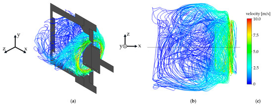
Figure 12.
Streamlines of the oil in the domain oil chamber for = 2000 rev/min, reference variant. (a) Streamlines of oil, with sectional view of the model. (b) Streamlines of oil, top view. (c) velocity scale.
3.2. Temperature Contour Plot
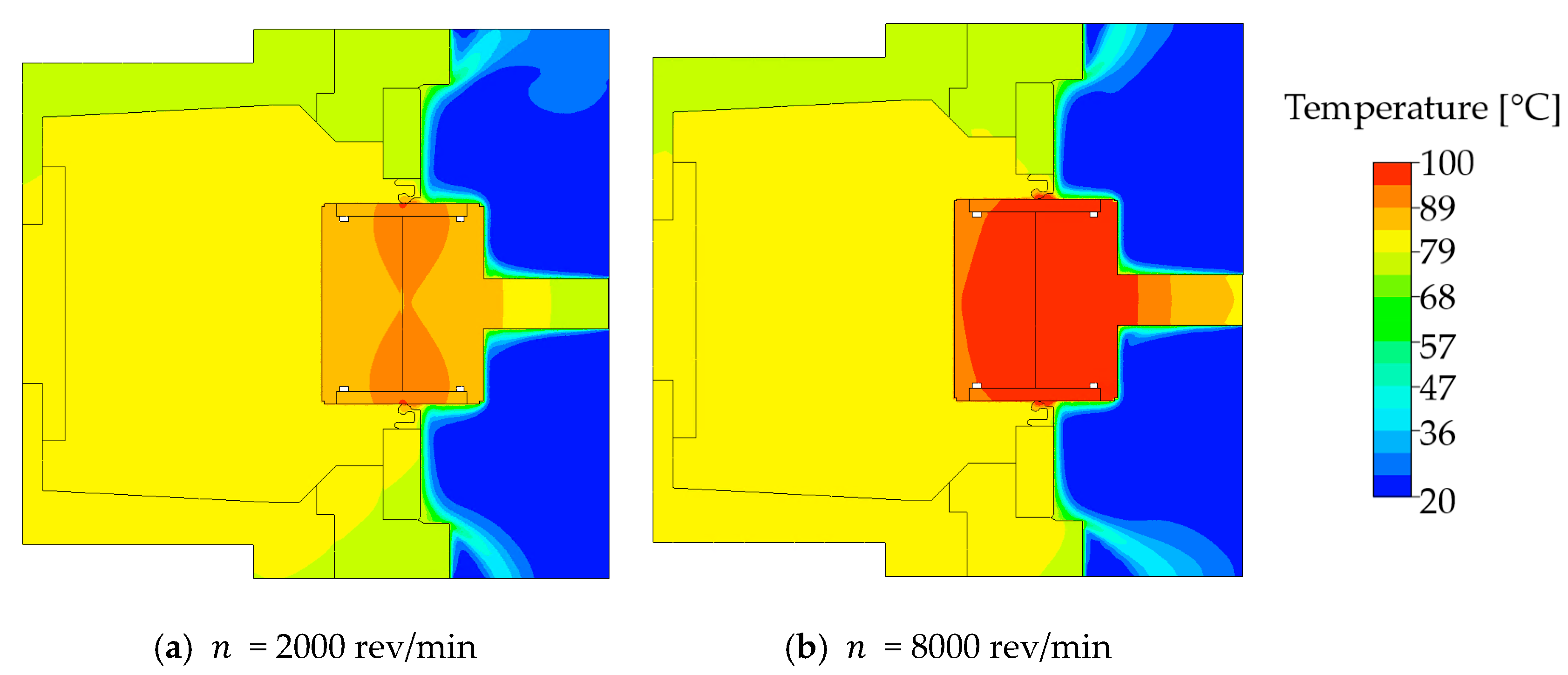
Figure 13 shows the temperature distribution in the cross-section of the reference variant for the rotational shaft speeds = 2000 rev/min and = 8000 rev/min.

Figure 13.
Contour plot, reference variant for (a) = 2000 rev/min; (b) = 8000 rev/min.
Due to the heat source applied as a boundary condition in the contact between the sealing ring and the shaft, the maximum temperature occurred in the sealing contact. Since this heat source was greater for higher shaft speeds, as demonstrated by Equation (17), the temperature was higher the higher the shaft speed was. Since the shaft made of steel conducts heated better than the seal made of elastomer, the generated heat was not evenly divided between the sealing ring and the shaft. A larger part of the heat generated in the sealing gap was applied to the shaft, and only a small part to the sealing ring; see Equations (19)–(21). Due to these material properties, the heat generated in the sealing contact was dissipated more towards the shaft than towards the seal.
The rational function describing the frictional torque , calculated using Equation (18), is used not only for the frictional torque of the sealing ring but also for the frictional torque of the bearings. The frictional torque of the bearings and, thus, the heat source caused by friction at the bearings, calculated using Equation (17), was different for each variant with bearings. Since the geometry of the cylindrical roller bearing in combination with the ball bearing was not symmetrical, as shown in Figure 6d, the frictional torque of the bearings was divided into one part generated by the ball bearing near the sealing ring and one part generated by the bearing distant from the seal. Thus, for the variants with bearings, eight additional parameters, four for each bearing, had to be defined to determine the frictional torques of the two bearings according to the rational function in Equation (18). By multiplying the frictional torque with the rotational shaft speed, the frictional heat was obtained, listed in Table 4. In addition, the four variants with bearings differed in the fill level of the oil in the domain oil chamber bearing, as shown in Figure 14. The input parameter oil fill level is also given in Table 4.
Table 4.
Variants with bearings: input parameters oil fill level and frictional heat, and the resulting temperature; = 2000 rev/min.
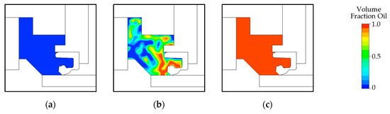
Figure 14.
Volume fraction of the oil in the domain oil chamber bearing; = 2000 rev/min. (a) Bea_X. (b) Bea_Ba and Bea_Cyl. (c) Bea_O.
The four parameters for determining the frictional torque of the sealing ring, calculated using Equation (18), were assumed to be identical for all variants, regardless of whether additional elements were simulated or not. Thus, the frictional heat generated in the contact area between the sealing ring and shaft surface was the same for all variants. This frictional heat generated was subdivided into the two parts and , shown in Equations (20) and (21). The temperature given in the last row in Table 4 is the temperature obtained from the simulation. This is the maximum temperature occurring on an interface between the rotary shaft seal (RSS) and the environment.
For the tapered roller bearing in the X-arrangement, there was only air in the volume between the bearing and the sealing ring, and the volume fraction of the oil is zero, as shown in Figure 14a. For the O-arrangement of the tapered roller bearing, the volume was completely filled with oil, as shown in Figure 14c, and in the case of the other two variants, it was half-filled with oil and half-filled with air, as shown in Figure 14b. These assumptions were based on experiences and observations during the experiments of the test bench.
The temperature distribution of the variants, with a bearings of = 2000 rev/min, are shown in Figure 15.
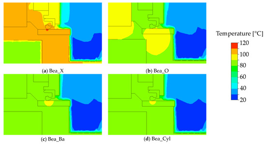
Figure 15.
Contour plots for = 2000 rev/min, variants with bearings: (a) X-arrangement; (b) O-arrangement; (c) ball-bearings; and (d) cylindrical roller bearings.
Due to its material properties, shown in Table 1, oil conducts heat better than air. In the simulation with the tapered roller bearings in the X-arrangement, there was pure air on both sides of the sealing ring and the heat generated in the sealing contact could, therefore, be dissipated less effectively. The highest frictional torque was measured on the test bench for the variant completely filled with oil, Bea_O, which is why the most frictional heat was added to the system here using the boundary condition; see Table 4. The measured frictional heat for the tapered roller bearings in the X-arrangement was only slightly lower. Since the volume between the sealing ring and the tapered roller bearings in the X-arrangement was completely filled with air and, therefore, conducted the heat worse, the simulation, nevertheless, resulted in the highest temperatures for Bea_X.
4. Discussion
The input parameter is given in the unit rev/min. With the diameter of the shaft, = 80 mm, the circumferential speed could be calculated in the unit m/s. Both notations are given in Table 5. Additionally, two different simulation results are listed in Table 5:
Table 5.
Simulation results and measurements of the reference variant, depending on the input parameter .
- ϑMax at RSS-shaft: These were the maximum values of the temperature in the contact area between the sealing ring and the rotating shaft; see Figure 16a.
 Figure 16. Temperature measurement procedure: (a) sealing ring with interfaces; (b) location of performed measurements.
 - ϑMax at RSS-environment: These were the maximum values of the temperature on one of the interfaces between the sealing ring and the environment; see Figure 16a.
There was only one contact interface between the sealing ring and the shaft: RSS–shaft. Multiple surfaces of the sealing ring were in contact with the environment. The interface which was designated as the RSS–environment interface is shown in Figure 16a. The simulation results were compared to the measured temperatures in Table 5. The measurements represent the mean value of at least three individual measurements.
The maximum temperature occurring in the entire model arose in the contact area, i.e., on the RSS–shaft interface. However, when measuring the temperatures on the test bench, the thermal imager was pointed at the contact area from the air side, as shown in Figure 16b. The temperatures directly in the sealing gap and, thus, on the interface between the sealing ring and the shaft, could not be measured with this method. Therefore, the temperatures resulting from the simulation that corresponded most to the measurements performed were not the highest temperatures occurring in the sealing contact, but the maximum temperatures at the interface between the sealing ring and the environment, the RSS–environment interface, as shown in Figure 16a. These temperatures from the simulation are, therefore, compared with the measurements in the following section.
4.1. Variants with Additional Elements
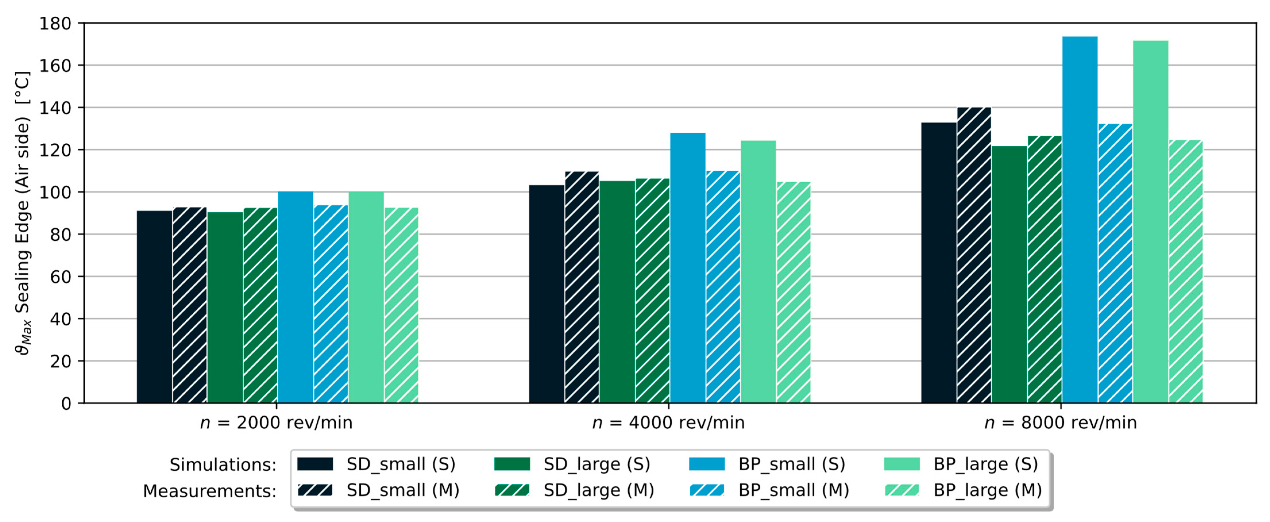
In Figure 17, the temperatures obtained from the simulation of the variants with the slinger disc and baffle plate are compared with the measurements. The simulation results are displayed in full color, and the temperatures obtained from the measurements are displayed hatched. The two variants with baffle plate deviated strongly from the measurement results. The temperature difference between the measurement results and the simulation results for the variant BP_large was almost 50 K for the shaft speed = 8000 rev/min. For the variants with the slinger disc, the temperature difference was generally much smaller, the maximum difference being about 10 K. A reason for the large temperature difference between the measurement and simulation for the variants with the baffle plate could be that the baffle plate was cut at the inner diameter for the experiments in order to attach a temperature sensor. This cut may have caused the oil to be better mixed near the sealing ring. The oil heated up through the frictional heat near the sealing contact, thus, mixed more quickly with the cooler oil further away from the sealing contact. Thus, the oil cooled down faster in the area near the sealing contact due to its better mixing with the cooler oil, which is why the measured temperatures were much lower than the temperatures obtained from the simulations.
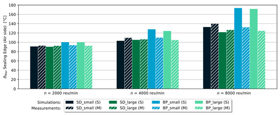
Figure 17.
Variants with slinger disc or baffle plate: simulation results (full colored) compared to the measured temperatures (hatched).
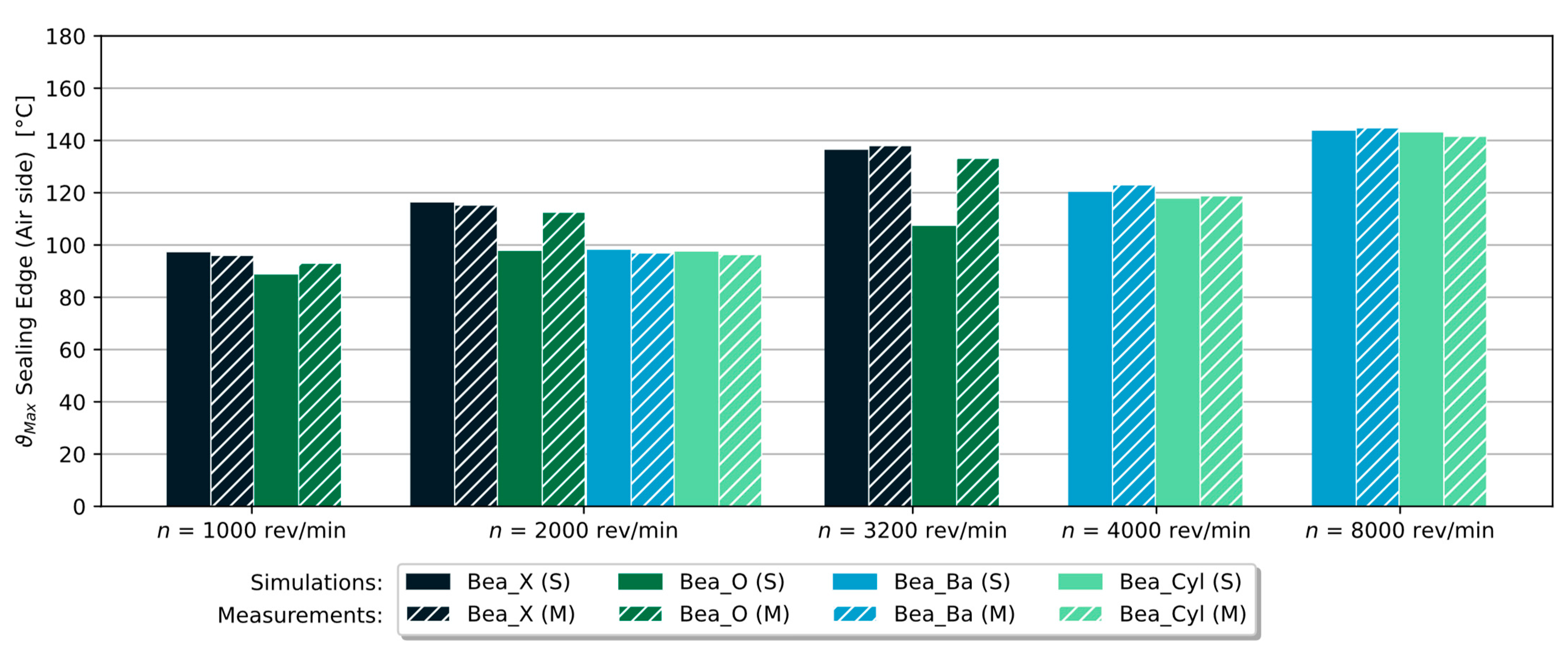
Figure 18 compares the temperature values obtained from the simulations with the measured temperatures for the different bearing arrangements. The rotational shaft speeds tested with the tapered roller bearings on the test bench were = 1000 rev/min, = 2000 rev/min and = 3200 rev/min. The ball bearings and cylindrical roller bearings were tested with = 2000 rev/min, = 4000 rev/min and = 6300 rev/min. The same shaft speeds were used for the simulations.

Figure 18.
Variants with bearings: simulation results (full colored) compared to the measured temperatures (hatched).
The largest temperature difference of approx. 26 K for = 3200 rev/min and approx. 15 K for = 2000 rev/min occurred for the tapered roller bearings in the O-arrangement. This difference may have been due to the fact that the frictional heat generated in the sealing contact was incorrectly assumed in the simulations: the frictional torque of the sealing ring was measured several times in the experiments with the reference variant, i.e., without additional elements and with a solid shaft. In these experiments, the oil chamber was filled with oil up to the center of the shaft. Based on these measured frictional torque values, the parameters in Equation (18) were determined. These parameters were identical for all the simulated variants. This means the frictional heat generated in the contact area between the sealing ring and the shaft was assumed to be the same for all the variants.
Due to the pumping effect of the bearings, the fluid was pumped towards the sealing ring for the O-arrangement of the tapered roller bearings. In the simulation, it was, therefore, assumed that the domain oil chamber bearing would be completely filled with oil. In the experiments, it was observed that this volume did indeed fill completely with oil. However, the bearing continued to pump oil even when the volume was already completely filled with oil, which could have resulted in a higher pressure on the sealing edge. The sealing edge may, therefore, have been pressed against the shaft on the oil side, which could have led to higher friction. Compared to the reference variant, the sealing edge would, thus, be pressed differently on the shaft surface for the O-arrangement of the tapered roller bearings due to the overpressure on the oil side. The parameters defined in the simulation model for determining the frictional heat in the sealing contact were based on the reference variant and were, therefore, incorrect for the O-arrangement of the tapered roller bearings. For all other simulated variants with bearings, the assumed parameters seem to be correct, as the measured values agreed well with the results from the simulations.
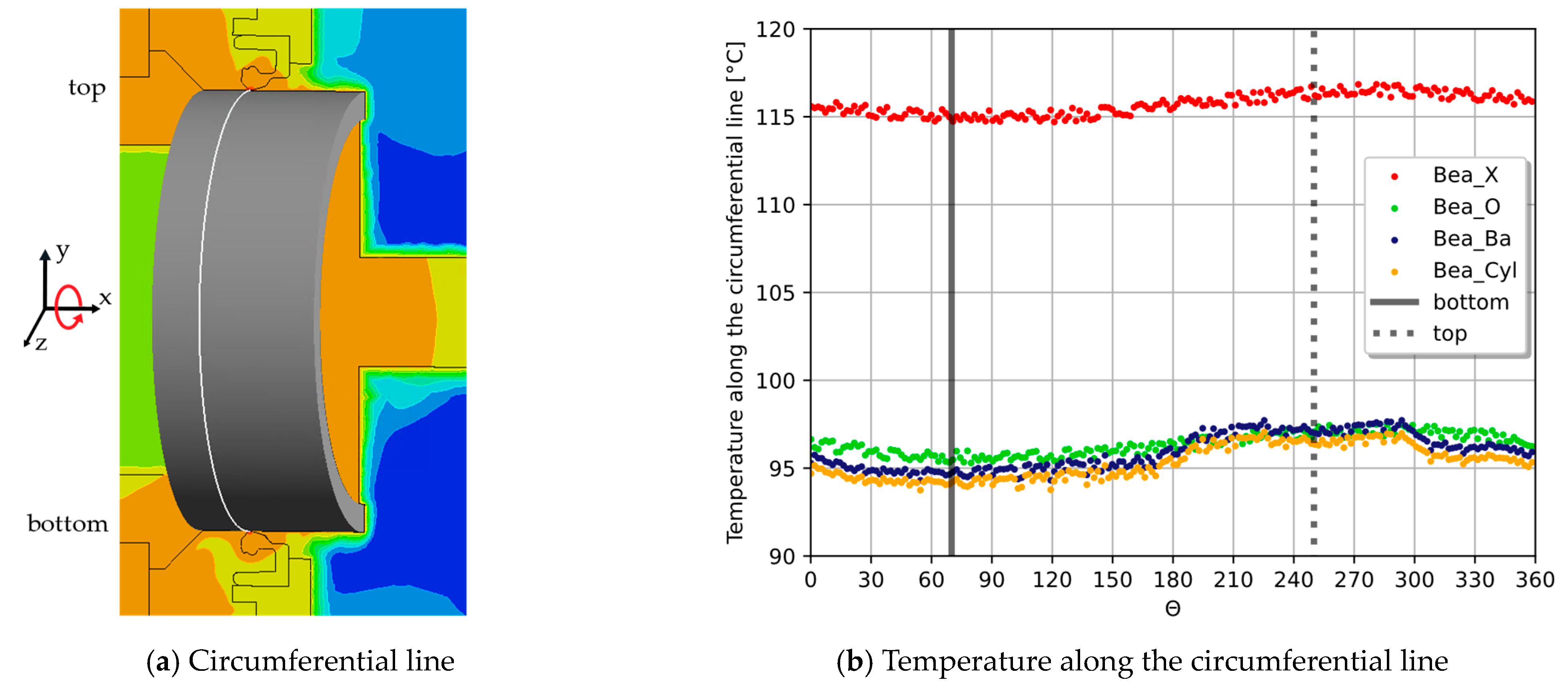
The rotating shaft distributed the oil in the oil chamber, but due to gravity, especially at low rotational shaft speeds, there was still more oil in the lower half of the oil chamber, as shown in Figure 11. Since oil conducts heat better than air, as shown in Table 1, the heat generated in the sealing contact was dissipated better in the lower area of the oil chamber. To analyze these fluctuations in a circumferential direction, a line was placed in the sealing contact around the circumference of the shaft sleeve, as shown in Figure 19a. On this line, the temperature was evaluated in steps of Θ = 1° for each variant with bearings and the rotational shaft speed = 2000 rev/min, as shown in Figure 19b. The two vertical dashed lines mark the two positions “top” and “bottom”. The position “top” refers to the location on the circumferential line with the most-positive y-coordinate. The position “bottom” analogously refers to the location on the line with the smallest y-coordinate. Due to the better thermal conductivity of the oil, the temperatures in the lower part and especially at the “bottom” position were generally slightly lower than the temperatures at the “top” position. For example, for the X-arrangement, the temperature varied between approx. 114.7 °C and 116.8 °C, as shown in Table 6. This temperature difference is negligible.

Figure 19.
Temperature distribution along a circumferential line: (a) contour plot with the line around the shaft sleeve; (b) temperature plot for = 2000 rev/min.
Table 6.
Minimum and maximum temperatures along the circumferential line in the sealing contact, = 2000 rev/min.
A second horizontal line 49 mm long and 0.7 mm below the sealing contact, was defined, shown in Figure 20a. At 200 equidistant data points across the line, the temperature was evaluated for the four variants with bearings, as shown in Figure 20b. The temperature plot over the x-coordinates of the horizontal line looks like a slightly asymmetrical Gaussian distribution curve, with the maximum at the position of the sealing contact.
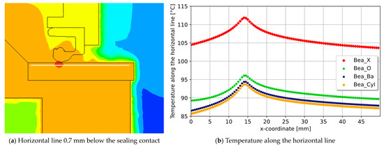
Figure 20.
Temperature distribution along the horizontal line: (a) contour plot with the horizontal line; (b) temperature plot for = 2000 rev/min.
4.2. Shaft Design
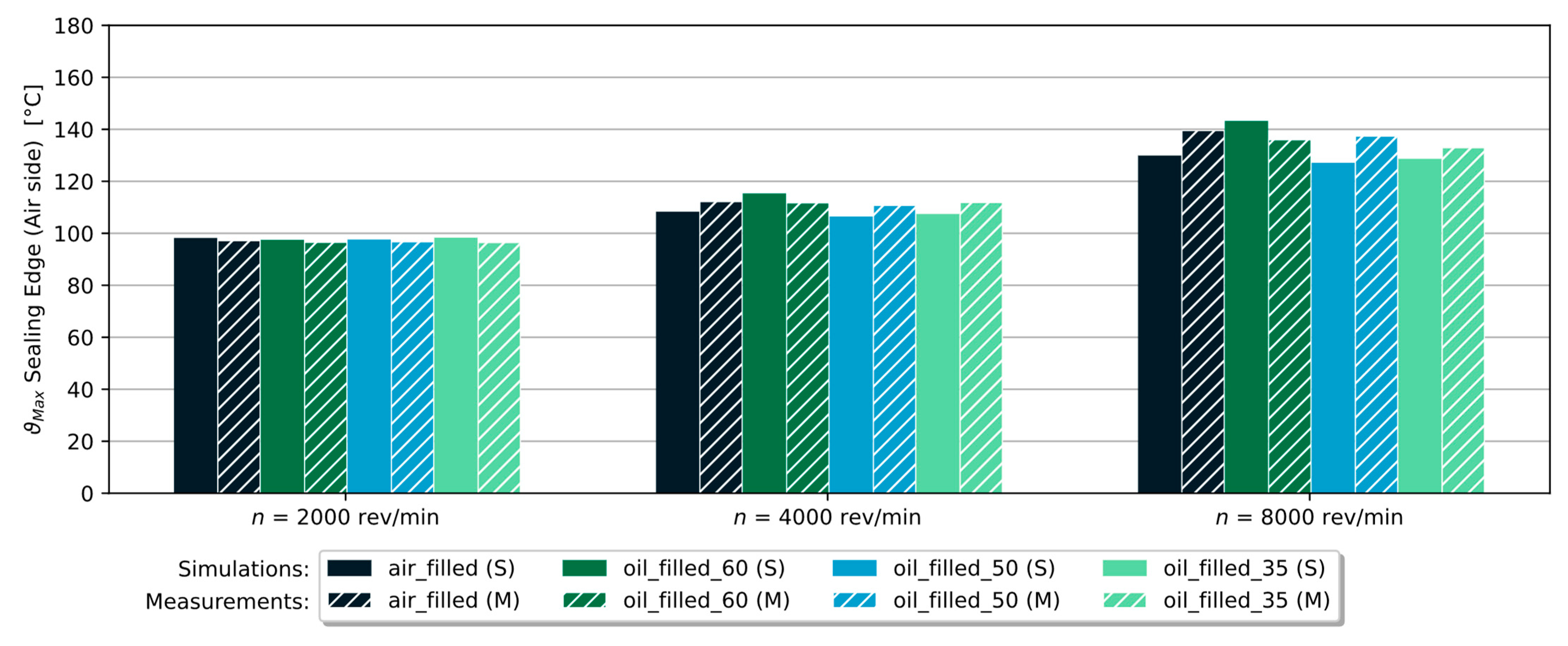
The simulation results for the three different rotational shaft speeds are compared to the measurements in Figure 21 for the variants with the hollow shaft design. The measured temperatures differed only slightly from the simulation results. For a rotational shaft speed of = 2000 rev/min, the measured temperatures were slightly lower than the simulation results.

Figure 21.
Hollow shaft: measured temperatures (hatched) compared to the simulation results (fully colored).
The temperatures obtained from the simulations of the shaft shoulder designs also fitted very well with the measured temperatures, as shown in Figure 22. At low rotational shaft speeds, very similar temperatures were measured for all four variants with the shoulder design. As the shaft speed increased, the measured temperature of the variant air_short was higher than those of the other variants. For the variant air_short, only very little material was available on the air side through which the heat could be transferred to the air. This could explain the higher temperature in both the simulation and the measurements of the variant air_short, compared to the other variants.
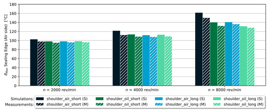
Figure 22.
Shaft with shoulder design: measured temperatures (hatched) compared to the simulation results (fully colored).
4.3. Accuracy of All Variants
In the simulations, an oil sump temperature of = 80 °C was assumed, since the oil was heated up to this temperature during the experiments using the test bench. During the experiments, the oil temperature was continuously measured, and adjusted if necessary, to ensure a constant temperature of = 80 °C. The measured and recorded oil temperatures, nevertheless, fluctuated between = 77 °C and = 85 °C. A temperature difference between the simulation and measurement of a few degrees could, for example, be due to the fluctuating oil-sump temperature. Small temperature differences are, therefore, negligible.
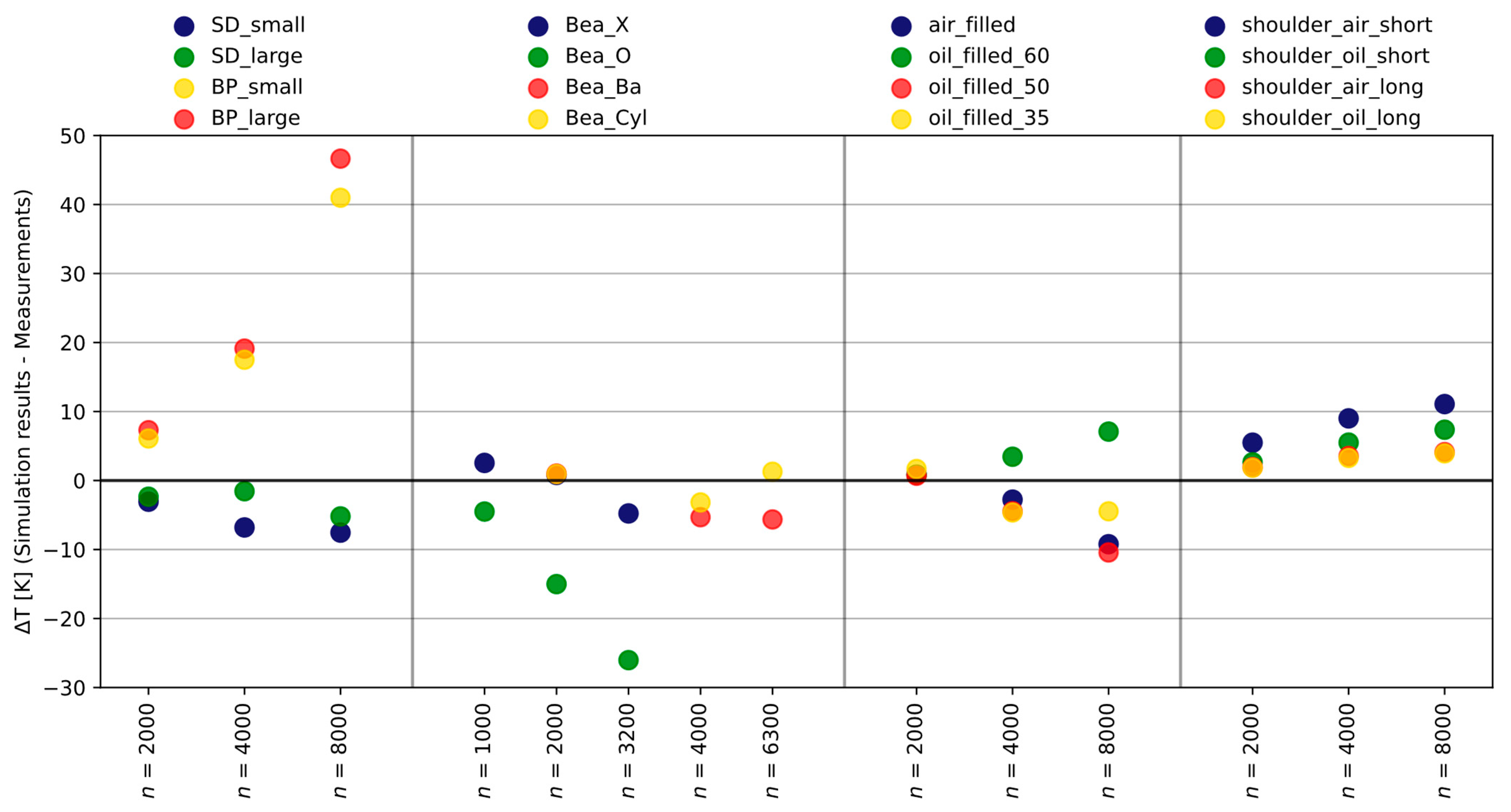
Figure 23 compares the temperatures obtained from the simulation with the measured temperatures of from all the variants. On the leftmost panel, the variants with the slinger disc or baffle plate are compared and, in the middle-left panel, the variants with bearings are compared. The variants with a hollow shaft design are compared in the middle-right panel, and on the rightmost panel, the variants with shaft shoulder designs are compared. Each panel is, furthermore, subdivided into the simulated rotational shaft speeds in rev/min. In general, the temperature difference between the measurement and simulation increased with the shaft speed.
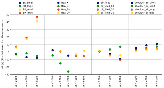
Figure 23.
Difference between the measured temperature and the temperature obtained from the simulation for all simulated variants.
For the variants with a slinger disc or baffle plate, two trends can be observed: For the variants with the slinger disc, all the measured temperatures were higher than the simulated temperatures, which was why the temperature difference ΔT was negative. For the variants with the baffle plate, it was the other way around: the simulations resulted in higher temperatures than the measurements, which is why the difference was positive overall. The largest deviation between the simulation and measurement was observed at a high shaft speed for the variants with the baffle plate. The deviations for the variants with bearings were small (ΔT < 10 K), except for the tapered roller bearings in the O-arrangement.
The difference between the temperatures obtained from the simulations and the measured temperatures was generally small for the variants with a hollow shaft. The temperature differences for the variants with a shaft shoulder design were all positive, meaning the measured temperatures were smaller than the temperatures from the simulations. Thus, the actual temperature was slightly underestimated in the simulation for these variants.
5. Conclusions
A parametric computational-fluid-dynamics simulation model was created in the software Ansys CFX 2021 R2, with which different variants can be computed in a short time. With this model, the maximum occurring temperatures in the contact area between the shaft and sealing ring can be determined for different variants, for example, for different geometries or materials. Moreover, the simulation model allows the determination of heat dissipation from the sealing contact to the surroundings for initial design ideas without a prototype. In this way, the surrounding geometry of a sealing ring can be optimally designed to achieve a longer product life. Regarding existing simulation models in recent years, the focus has, rather, been on the sealing gap itself, which was why many influencing factors (e.g., heat convection in oil, and air flow) could not be considered. The simulation model created in this work takes nearly all influencing factors, shown in Figure 2, into account, with the possibility of including even more.
A reference configuration and, additionally, 16 different variants, were simulated for different rotational shaft speeds. All simulated variants were additionally tested on the test bench, and the measured temperatures were compared to the temperatures obtained from the simulations. For this purpose, the maximum temperature at an interface between the sealing ring and the environment was used. Based on the comparison of the measurements with the simulation results, conclusions could be drawn about which of the simplifications used in the simulation led to accurate simulation results, as summarized in Table 7.
Table 7.
Simplifications made in the simulations.
For all the simulated variants, the same frictional heat generated in the contact area between the sealing ring and shaft was introduced into the simulation model as a boundary condition (No. 1 and No. 2). This frictional heat was based on the frictional torque measured on the test bench for the reference variant and was found to not be transferable to the variant with tapered roller bearings in the O-arrangement. For all other simulated variants, the simplification No. 2 proved to be a valid approach. In the case of the tapered roller bearings in the O-arrangement, the exact value of the frictional torque would have been needed in order to be able to compare the simulation results with the measured values.
The temperatures measured in the experiments with the slinger disc could be reproduced well in the simulations. In the simulations with baffle plates, it became apparent how great the influence of the design of the components surrounding the sealing ring was for the contact temperature between the sealing ring and shaft. Due to the simplification of the geometry of the baffle plate (No. 5), the measurement results could not be confirmed with the simulations.
Using only two varying input parameters to model the different bearings (No. 3) has been proven to be a valid approach. With these input expressions, the pumping effect of the bearings could be modeled well for the tapered roller bearings in the X-arrangement, the ball bearings and the cylindrical roller bearings. It has also been shown that the differences in the geometries of the bearings were negligible and, therefore, one geometry model is sufficient for modeling all variants with bearings (No. 6), but only if both the pumping effect of the bearings and the frictional torque of the bearings are known, since both must be included as input variables.
Despite not considering the air inside the air-filled hollow shaft (No. 7), and assuming that the boundaries of the air-filled hollow shaft were adiabatic to the volume inside, the simulation yielded good results. In the case of the variants with an oil-filled hollow shaft, the temperatures obtained from the simulations matched the measured temperatures well. The measured temperatures were slightly underestimated in the simulations of the variants with the shoulder design; nevertheless, the temperatures obtained from the simulation fitted well with the measured temperatures.
Author Contributions
Conceptualization, J.H. and J.G.; methodology, S.F.; validation, C.O. and S.F.; investigation, J.H., J.G., C.O. and S.F.; writing—original draft preparation, J.H.; writing—review and editing, J.H., J.G., C.O. and S.F.; visualization, J.H.; supervision, F.B. All authors have read and agreed to the published version of the manuscript.
Funding
This IGF research project 21587 N/1 of the Forschungskuratorium Maschinenbau e.V. (FKM, Mechanical Engineering Research Forum) was funded by the AiF as a support of the Industrielle Gemeinschaftsforschung (IGF, Industrial Collective Research), by the Bundesministerium für Wirtschaft und Klimaschutz der Bundesrepublik Deutschland (BMWK, Federal Ministry for Economic Affairs and Climate Action) on the basis of the decision by the German Bundestag.
Institutional Review Board Statement
Not applicable.
Informed Consent Statement
Not applicable.
Data Availability Statement
The data presented in this study are available on request from the corresponding author.
Conflicts of Interest
The authors declare no conflict of interest. The funders had no role in the design of the study; in the collection, analyses, or interpretation of data; in the writing of the manuscript; or in the decision to publish the results.
Nomenclature
| Symbol | Description | Unit |
| specific heat capacity | J/(kg·K) | |
| transport variable, volume-of-fluid (VOF) method | - | |
| transport variable for the air phase, VOF | - | |
| transport variable for the oil phase, VOF | - | |
| shaft diameter | mm | |
| heat partition factor | - | |
| g | gravitational acceleration | m/s2 |
| enthalpy | J/kg | |
| incoming enthalpy | J/kg | |
| outgoing enthalpy | J/kg | |
| total enthalpy | J/kg | |
| oil fill level in the domain oil chamber bearing | mm | |
| mass flow | kg/s | |
| molar mass | kg/mol | |
| frictional torque | N·m | |
| rotational shaft speed | rev/min | |
| pressure | Pa | |
| current air pressure | Pa | |
| heat flux density | kg/s3 | |
| heat flux | W | |
| frictional heat flux | W | |
| frictional heat flux applied to the seal | W | |
| frictional heat flux applied to the shaft | W | |
| universal gas constant | J/(mol·K) | |
| optional source term in the momentum equations | kg/(s2·m3) | |
| source term for buoyancy | kg/(s2·m3) | |
| volumetric heat source | kg/(s3·m2) | |
| time | s | |
| current air temperature | K | |
| temperature | °C | |
| air temperature | °C | |
| current oil temperature | °C | |
| initial temperature | °C | |
| fluid temperature | °C | |
| wall temperature | °C | |
| flow velocity vector field | m/s | |
| circumferential velocity | m/s | |
| material parameter in the Vogel equation | Pa·s | |
| material parameter in the Vogel equation | K | |
| Vogel temperature | K | |
| working current | W | |
| heat transfer coefficient | W·K/m2 | |
| dynamic viscosity of the air | Pa·s | |
| dynamic viscosity of the oil | Pa·s | |
| thermal conductivity | W/(m·K) | |
| thermal conductivity of the air | W/(m·K) | |
| thermal conductivity of the sealing ring material | W/(m·K) | |
| thermal conductivity of the shaft material | W/(m·K) | |
| density | kg/m3 | |
| air density | kg/m3 | |
| oil density | kg/m3 | |
| shear-stress tensor | Pa |
References
- Bauer, F. Federvorgespannte-Elastomer-Radial-Wellendichtungen; Springer Fachmedien Wiesbaden: Wiesbaden, Germany, 2021; ISBN 978-3-658-32921-1. [Google Scholar]
- ISO 6194-1; Rotary Shaft Lip-Type Seals Incorporating Elastomeric Sealing Elements—Part 1: Nominal Dimensions and Tolerances. International Organization for Standardization, Beuth Verlag GmbH: Berlin, Germany, 2007.
- DIN 3760; Rotary Shaft Lip Type Seals. Norelem: Markgröningen, Germany, 1996.
- Kammüller, M. Zur Abdichtwirkung von Radial-Wellendichtringen; Berichte aus dem Institut für Maschinenelemente und Gestaltungslehre; Inst. für Maschinenelemente und Gestaltungslehre: Stuttgart, Germany, 1986; ISBN 978-3-921920-19-0. [Google Scholar]
- Kawahara, Y.; Abe, M.; Hirabayashi, H. An Analysis of Sealing Characteristics of Oil Seals. A S L E Trans. 1980, 23, 93–102. [Google Scholar] [CrossRef]
- Leeuwen, H.J.; Wolfert, M.A. The Sealing and Lubrication Principles of Plain Radial Lip Seals: An Experimental Study of Local Tangential Deformations and Film Thickness. Tribol. Ser. 1997, 32, 219–232. [Google Scholar]
- Feldmeth, S.; Bauer, F.; Haas, W. Abschätzverfahren Für Die Kontakttemperatur Bei Radial-Wellendichtungen. In Sealing Technology—Indispensable; Fachverband Fluidtechnik, Universität Stuttgart, Eds.; Fachverband Fluidtechnik im VDMA e.V: Frankfurt am Main, Germany, 2016; ISBN 978-3-8163-0684-9. [Google Scholar]
- Feldmeth, S.; Bauer, F.; Haas, W. Simulation of the Temperature Field in Radial Lip Seals Using a Multiscale Approach. In Seminar: Best Practices for Thermal Analyses and Heat Transfer; NAFEMS Deutschland, Österreich, Schweiz GmbH, Eds.; NAFEMS Deutschland, Österreich, Schweiz GmbH: Bernau am Chiemsee, Germany, 2014. [Google Scholar]
- Feldmeth, S.; Braeurer, P.; Franke, J.; Bauer, F. Temperature Measurement in the Sealing Contact—Sealing Systems Are Getting Smarter. In XXII Dichtungskolloquium; Riedl, A., Ed.; Vulkan Verlag GmbH: Münster, Germany, 2021. [Google Scholar]
- Brink, R.V. The Heat Load of an Oil Seal. In Proceedings of the 6th International Conference on Fluid Sealing, München, Germany, 27 February–2 March 1973. Paper C1. [Google Scholar]
- Upper, G. Dichtlippentemperatur von Radial-Wellendichtringen. In Theoretische Und Experimentelle Untersuchung; University of Karlsruhe: Karlsruhe, Germany, 1968. [Google Scholar]
- Universität Stuttgart InsECT Calculationtool. Version Beta-18.10.08. Available online: https://insect.ima.uni-stuttgart.de (accessed on 20 July 2023).
- Feldmeth, S.; Bauer, F.; Haas, W. Abschätzung der Kontakttemperatur bei Radial-Wellendichtungen mit der selbstentwickelten Open-Source-Software InsECT. In Proceedings of the SMK 2016, Schweizer Maschinenelemente Kolloquium, Rapperswil, Switzerland, 22–23 November 2016; TUDpress: Dresden, Germany, 2016. [Google Scholar]
- Grün, J.; Gohs, M.; Bauer, F. Multiscale Structural Mechanics of Rotary Shaft Seals: Numerical Studies and Visual Experiments. Lubricants 2023, 11, 234. [Google Scholar] [CrossRef]
- Grün, J.; Feldmeth, S.; Bauer, F. Computational Fluid Dynamics of the Lubricant Flow in the Sealing Gap of Rotary Shaft Seals. In Proceedings of the M2D2022—9th International Conference on Mechanics and Materials in Desig, Funchal, Portugal, 26–30 June 2022; Gomes, J.F.S., Meguid, S.A., Eds.; pp. 1035–1050. [Google Scholar]
- Stakenborg, M.J.L. On the Sealing Mechanism of Radial Lip Seals. Tribol. Int. 1988, 21, 335–340. [Google Scholar] [CrossRef]
- Wenk, J.F.; Scott Stephens, L.; Lattime, S.B.; Weatherly, D. A Multi-Scale Finite Element Contact Model Using Measured Surface Roughness for a Radial Lip Seal. Tribol. Int. 2016, 97, 288–301. [Google Scholar] [CrossRef]
- Grün, J.; Feldmeth, S.; Bauer, F. The Sealing Mechanism of Radial Lip Seals: A Numerical Study of the Tangential Distortion of the Sealing Edge. Tribol. Mater. 2022, 1, 165–166. [Google Scholar] [CrossRef]
- Salant, R.F. Soft Elastohydrodynamic Analysis of Rotary Lip Seals, Proceedings of the Institution of Mechanical Engineers. Part C J. Mech. Eng. Sci. 2010, 224, 2637–2647. [Google Scholar] [CrossRef]
- Feldmeth, S.; Bauer, F.; Haas, W. Untersuchung Des Einflusses Verschiedener Versuchskonfigurationen Auf Die Dichtspalttemperatur Bei Radial-Wellendichtungen Mittels CHT-Simulation. In NAFEMS Magazin, Ausgabe 29; NAFEMS Deutschland, Österreich, Schweiz GmbH: Bernau am Chiemsee, Germany, 2014. [Google Scholar]
- Schwarze, R. CFD-Modellierung: Grundlagen und Anwendungen bei Strömungsprozessen; Springer Vieweg: Berlin/Heidelberg, Germany, 2013; ISBN 978-3-642-24377-6. [Google Scholar]
- Tu, J.; Yeoh, G.H.; Liu, C. Governing Equations for CFD—Fundamentals. In Computational Fluid Dynamics; Elsevier: Amsterdam, The Netherlands, 2008; pp. 65–125. ISBN 978-0-7506-8563-4. [Google Scholar]
- ANSYS CFX-Solver Theory Guide; ANSYS, Inc.: Canonsburg, PA, USA, 2009.
- VDI. VDI-Wärmeatlas, 11th ed.; Springer: Berlin/Heidelberg, Germany, 2013; ISBN 978-3-642-19980-6. [Google Scholar]
- Ungarish, M. Hydrodynamics of Suspensions: Fundamentals of Centrifugal and Gravity Separation; Springer: Berlin, Germany; New York, NY, USA, 1993; ISBN 978-3-540-54762-4. [Google Scholar]
- Gidaspow, D. Multiphase Flow and Fluidization: Continuum and Kinetic Theory Descriptions; Academic Press: Boston, MA, USA, 1994; ISBN 978-0-12-282470-8. [Google Scholar]
- Freudenberg FST GmbH Produktdatenblatt Radialwellendichtungen BAUM 75 FKM 585 Bauform. In eCatalog Simmerringe Und Rotationsdichtungen. 2020. Available online: https://Api.Fst.Com/Assets/Productdatasheet_de_baum.Pdf (accessed on 8 July 2023).
- IBC Wälzlager GmbH. Deutschland IBC Hochpräzisions-Wälzlager, High Precision Bearings; Katalog der IBC Wälzlager GmbH: Solms, Germany, 2010; p. 186. [Google Scholar]
- DIN German Institute for Standardization DIN EN ISO 3838: Determination of Density or Relative Density; Beuth Verlag GmbH: Berlin, Germany, 2004.
- Feldmeth, S.; Olbrich, C.; Bauer, F. Influence of Lubricants on the Thermal Behaviour of Rotary Shaft Seals. In Sealing Technology—Old School and Cutting Edge; Fachverband Fluidtechnik, Universität Stuttgart, Eds.; Fachverband Fluidtechnik im VDMA e.V: Frankfurt am Main, Germany, 2022. [Google Scholar]
- Laukotka, E. FVA-Heft 660. In Referenzöle—Datensammlung; Forschungsvereinigung Antriebstechnik: Frankfurt, Germany, 2007. [Google Scholar]
- DIN 53017; Viscometry: Determination of the Temperature Coefficient of Viscosity. Beuth Verlag GmbH: Berlin, Germany, 1993.
- Fulcher, G.S. Analysis of recent measurements of the viscosity of glasses. J. Am. Ceram. Soc. 1925, 8, 339–355. [Google Scholar] [CrossRef]
- Menter, F.R. Two-Equation Eddy-Viscosity Turbulence Models for Engineering Applications. AIAA J. 1993, 32, 1598–1605. [Google Scholar] [CrossRef]
- Blazek, J. Computational Fluid Dynamics: Principles and Applications, 2nd ed.; Elsevier: Amsterdam, The Netherlands; San Diego, CA, USA, 2005; ISBN 978-0-08-044506-9. [Google Scholar]
- Katopodes, N.D. Turbulent Flow. In Free-Surface Flow; Elsevier: Amsterdam, The Netherlands; San Diego, CA, USA, 2019; pp. 566–650. ISBN 978-0-12-815489-2. [Google Scholar]
- Ansys CFX-Solver Modeling Guide; Release 2021 R2 2021; ANSYS, Inc.: Canonsburg, PA, USA, 2021.
- Kunstfeld, T.; Haas, W. Dichtungsumfeld: Einfluss Des Bespritzungs- Und Luftseitigen Umfeldes Auf Die Dichtwirkung von Radial-Wellendichtungen: Abschlussbericht FKM Vorhaben Nr. 236; Forschungshefte, Forschungskuratorium Maschinenbau e.V. (FKM); Forschungskuratorium Maschinenbau e.V.: Frankfurt am Main, Germany, 2001; Heft 261. [Google Scholar]
- Schaeffler Technologies AG & Co. KG. Wälzlagerpraxis: Handbuch zur Gestaltung und Berechnung von Wälzlagerungen, 4th ed.; Antriebstechnik; Vereinigte Fachverl: Mainz, Germany, 2015; p. 455. ISBN 978-3-7830-0401-4. [Google Scholar]
- Jung, S.; Daubner, A.; Haas, W. Measurement and Simulation of Two-Phase Flow in Sealing Application. In Sealing Technology—Indispensable; Fachverband Fluidtechnik, Universität Stuttgart, Eds.; Fachverband Fluidtechnik im VDMA e.V: Frankfurt am Main, Germany, 2016. [Google Scholar]


Disclaimer/Publisher’s Note: The statements, opinions and data contained in all publications are solely those of the individual author(s) and contributor(s) and not of MDPI and/or the editor(s). MDPI and/or the editor(s) disclaim responsibility for any injury to people or property resulting from any ideas, methods, instructions or products referred to in the content. |
© 2023 by the authors. Licensee MDPI, Basel, Switzerland. This article is an open access article distributed under the terms and conditions of the Creative Commons Attribution (CC BY) license (https://creativecommons.org/licenses/by/4.0/).