
Enhancing Olive Phenology Prediction: Leveraging Market Basket Analysis and Weighted Metrics for Optimal Feature Group Selection


Abstract
:1. Introduction
2. Materials and Methods
2.1. Data Set

| Abbreviated | Original Features | Predictor | Data | Resolution |
|---|---|---|---|---|
| Feature Name | Type | Source | (km) | |
| DOY | Day of year | Time | ||
| mean temp | Average air temperature at 2 m height (daily average) | Meteo | ERA 5 | ∼28 |
| min temp | Minimal air temperature at 2 m height (daily minimum) | Meteo | ERA 5 | ∼28 |
| max temp | Maximal air temperature at 2 m height (daily maximum) | Meteo | ERA 5 | ∼28 |
| dewp temp | Dewpoint temperature at 2 m height (daily average) | Meteo | ERA 5 | ∼28 |
| total precip | Total precipitation (daily sums) | Meteo | ERA 5 | ∼28 |
| surface pressure | Surface pressure (daily average) | Meteo | ERA 5 | ∼28 |
| sea level | Mean sea-level pressure (daily average) | Meteo | ERA 5 | ∼28 |
| wind u | Horizontal speed of air moving towards the east, | |||
| at a height of 10 m above the surface of Earth. | Meteo | ERA 5 | ∼28 | |
| wind w | Horizontal speed of air moving towards the north. | Meteo | ERA 5 | ∼28 |
| EVI | Enhanced vegetation index (EVI) generated from the | 006 MOD09GA | ||
| Near-IR, red, and blue bands of each scene. | MODIS | EVI | 1 km | |
| NDVI | Normalized difference vegetation index generated | 006 MOD09GA | ||
| from the near-IR and red bands of each scene. | MODIS | NDVI | 1 km | |
| RED | Red surface reflectance (sur refl b01) | MODIS | 006 MOD09GQ | 0.25 km |
| NIR | NIR surface reflectance (sur refl b02) | MODIS | 006 MOD09GQ | 0.25 km |
| sur refl b03 | Blue surface reflectance, 16-day frequency | MODIS | 006 MOD13Q1 | 0.25 km |
| sur refl b07 | MIR surface reflectance, 16-day frequency | MODIS | 006 MOD13Q1 | 0.25 km |
| view zenith | View zenith angle, 16-day frequency | MODIS | 006 MOD13Q1 | 0.25 km |
| solar zenith | Solar zenith angle, 16-day frequency | MODIS | 006 MOD13Q1 | 0.25 km |
| rel azim | Relative azimuth angle, 16-day frequency | MODIS | 006 MOD13Q1 | 0.25 km |
| lat | Latitude | Spatial | ||
| lon | Longitude | Spatial | ||
| slope | Landform classes created by combining the ALOS CHILI | |||
| and ALOS mTPI data sets. | Spatial | ALOS Landform | ||
| Created features | ||||
| GDD | Growing degree day from GEE temperature measurements; t is base temperature used. | |||
| precip cum | Precipitation accumulated from the first of January until DOY. | |||
| EVIcum | EVI accumulated from the first of January until DOY. | |||
| NDVIcum | NDVI accumulated from 1 January until DOY. | |||
| REDcum | RED accumulated from 1 January until DOY. | |||
| NIRcum | NIR accumulated from 1 January until DOY. | |||
| RMSE | Feature List |
|---|---|
| Mean | |
| 0.5857 | slope, sea level, NDVI, lat, cum precip, surface pressure |
| 0.5865 | EVI, slope, sea level, lat, cum precip, surface pressure, mean temp |
| 0.5877 | EVI, slope, sea level, lat, cum precip, surface pressure |
| 0.5879 | slope, sea level, lat, cum precip, surface pressure |
| 0.5885 | slope, sea level, lat, cum precip, mean temp, GDD |
| 0.5887 | EVI, slope, sea level, lat, cum precip, mean temp, GDD |
| 0.5897 | EVI, slope, min temp, sea level, lat, cum precip, surface pressure |
| 0.5904 | EVI, slope, sea level, lat, surface pressure, mean temp |
| 0.5905 | slope, sea level, lat, cum precip, surface pressure, mean temp |
| 0.5905 | EVI, slope, sea level, NDVI, lat, cum precip, mean temp, GDD |
| 0.5908 | EVI, slope, min temp, sea level, lat, cum precip, surface pressure, GDD |
| 0.5911 | slope, min temp, sea level, NDVI, lat, cum precip, surface pressure, GDD |
| 0.5911 | slope, sea level, NDVI, lat, cum precip, surface pressure, GDD |
| 0.5915 | EVI, slope, min temp, sea level, lat, cum precip, mean temp, GDD |
| 0.5916 | EVI, slope, min temp, sea level, lat, cum precip, GDD |
| 0.5916 | slope, sea level, NDVI, lat, cum precip, surface pressure, mean temp, GDD |
| 0.5917 | slope, min temp, sea level, lat, cum precip, GDD |
| 0.5919 | EVI, slope, sea level, NDVI, lat, cum precip, surface pressure, mean temp, GDD |
| 0.5924 | EVI, slope, min temp, sea level, NDVI, lat, cum precip, surface pressure, GDD |
| 0.5924 | EVI, slope, sea level, NDVI, lat, cum precip, surface pressure |
| 0.5926 | slope, min temp, sea level, NDVI, lat, cum precip, surface pressure, mean temp, GDD |
| 0.5927 | EVI, slope, min temp, sea level, lat, mean temp, GDD |
| 0.5927 | slope, sea level, NDVI, lat, cum precip, surface pressure, mean temp |
| 0.5931 | EVI, slope, min temp, sea level, NDVI, lat, cum precip, GDD |
| 0.5931 | EVI, slope, sea level, NDVI, lat, cum precip, surface pressure, mean temp |
2.2. Methodology
2.2.1. Association Metrics
- Metric 1 (M1): The weight assigned to each edge , symbolizing the connection between two features x, y, is directly proportional to the Root Mean Square Error (RMSE) mean values presented in the ranked quantities in Table 2. Computation of this weight involves the aggregation of the average RMSE, which is accomplished by summing the corresponding values across all combinations in which the two features overlap x, y, as detailed by Equation (1). The outcome of employing this association metric M1 is the generation of an undirected weighted graph.
- Metric 2 (M2): In Market basket analysis, the associations between products are unveiled by analyzing combinations of products that frequently appear in transactions. Among the most commonly used metrics, the support, confidence and lift metrics are often used to justify strategic decisions in a marketing campaign, or product rearrangement in stores [23]:
- -
- Support: this metric quantifies the proportion of combinations in the data set containing a specific item. It represents the ratio of collections containing the itemset to the total number of combinations in the data set.
- -
- Confidence: it measures the proportion of collections that contain the antecedent x that also contains the consequent y. It is calculated as the ratio of the number of collections that contain both the antecedent x and the consequent y to the number of combinations that contain the antecedent x.
- -
- Lift: it calculates the ratio of the analyzed support to the expected support under the assumption of independence between the antecedent and the consequent. It indicates how likely the consequent is to occur when the antecedent is present compared to when the antecedent is absent. It is calculated as the confidence ratio of to support the consequent y.
2.2.2. Graph Network Analysis
- Degree Centrality: The degree of a node is the number of edges that are adjacent to the node, multiplied by corresponding weights define in Section 2.2.1.
- PageRank Centrality: An iterative algorithm that measures the importance of each node within the network. The page rank values are the values in the eigenvector with the highest corresponding eigenvalue of a normalized adjacency matrix derived from the graph [29].
- Modularity: A high modularity score indicates sophisticated internal structure. This structure, often called a community structure, describes how the the network is compartmentalized into sub-networks. These sub-networks (or communities) have been shown to have significant real-world meaning [30].
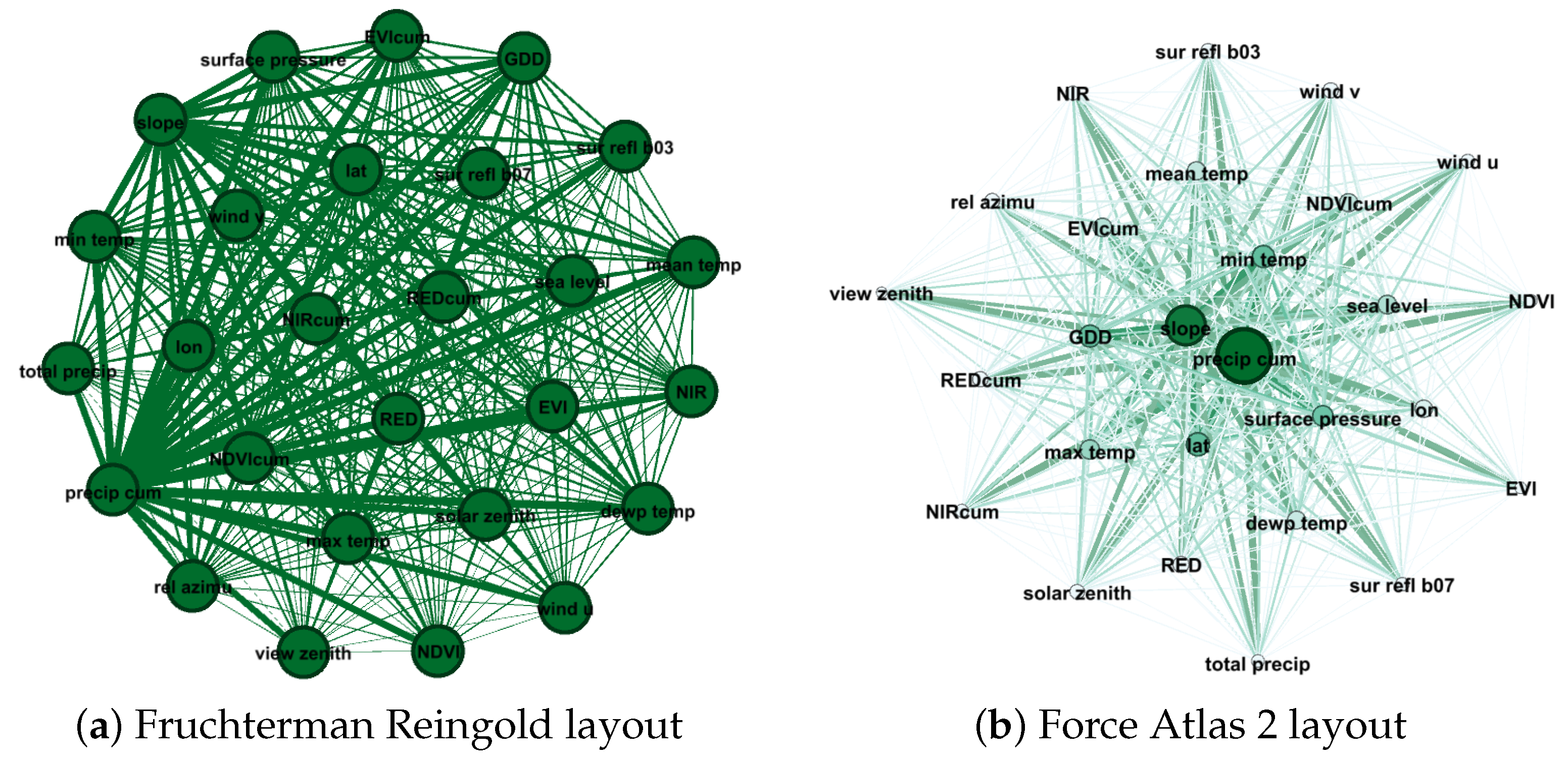
- Fruchterman Reingold: The Fruchterman-Reingold Algorithm is a force-directed layout algorithm. The idea of a force-directed layout algorithm is to consider a force between any two nodes. In this algorithm, the nodes are represented by steel rings and the edges are springs between them. The attractive force is analogous to the spring force and the repulsive force is analogous to the electrical force. The basic idea is to minimize the energy of the system by moving the nodes and changing the forces between them [31].
- Force Atlas 2: The main property of this force-directed layout consists of its implementation of distinct methods such as the Barnes Hut simulation, degree-dependent repulsive force, and local and global adaptive temperatures [32].
2.3. Validation Procedure
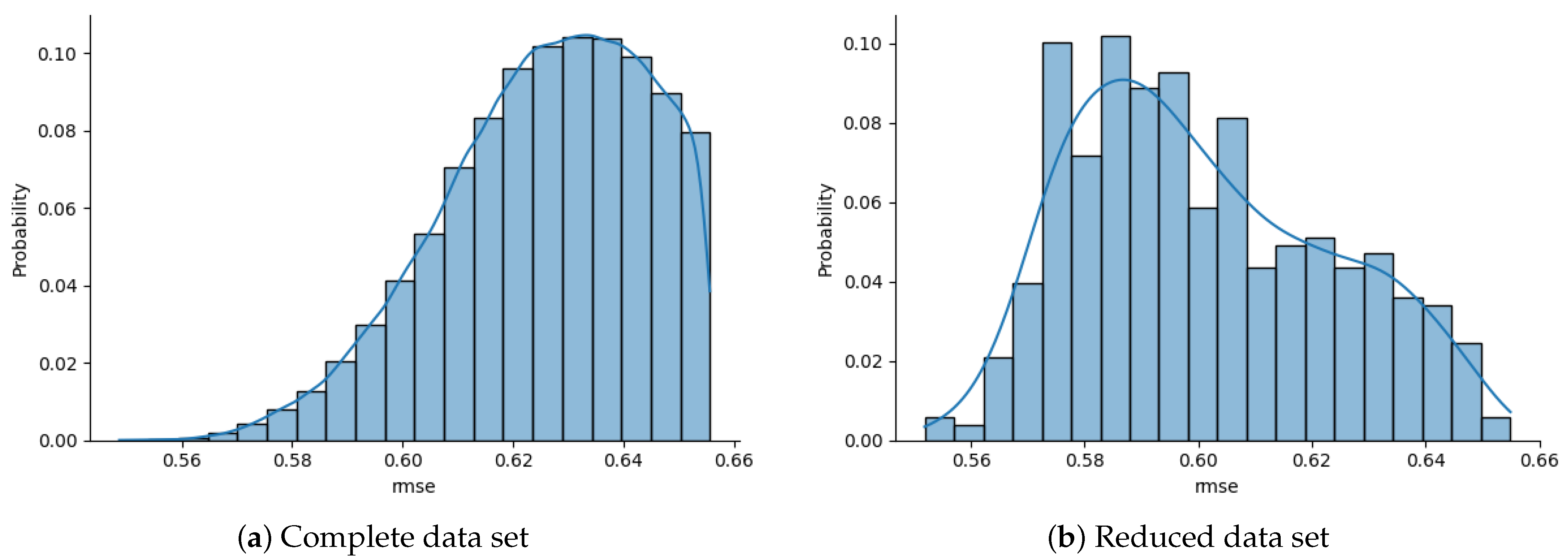
3. Results
3.1. Association Metrics
3.1.1. M1 Based Feature Association
3.1.2. M2 Based Feature Association
3.2. Network Visualization
3.3. Validation
- Feature Core: accumulated precipitation, maximal air temperature, latitude and sea level pressure.
- G1: Feature Core, slope, minimal air temperature
- G2: Feature Core, dewpoint temperature, accumulated RED.
- G3: GDD, NIRcum, EVIcum, REDcum, NDVIcum, precip cum
- G4: GDD, NIRcum, EVIcum, solar zenith, NDVIcum, mean temperature
- G5: sea level pressure, GDD, slope, wind u, blue surface reflectance, dewpoint temperature
4. Discussion
5. Conclusions
Author Contributions
Funding
Institutional Review Board Statement
Informed Consent Statement
Data Availability Statement
Conflicts of Interest
Abbreviations
| GDD | Growing degree days. |
| MBA | Market Basket Analysis. |
| BBCH | Biologische Bundesanstalt, Bundessortenamt, und CHemische Industrie. |
| DOY | Day Of Year. |
| EVI | Enhanced vegetation index. |
| NDVI | Normalized difference vegetation index. |
| GEE | Google Earth Engine. |
| RMSE | Root-mean-square deviation. |
| M1 | Metric 1, 1-RMSE weight proportional metric. |
| M2 | Metric 2, MBA-derived metric |
| G1 | Group 1, feature grouping derived from M1. |
| G2 | Group 2, feature grouping derived from M2. |
| G3 | Group 3, feature grouping derived from Pearson correlation coefficient. |
| G4 | Group 4, feature grouping derived from Mutual Info Regression. |
| G5 | Group 5, feature grouping derived from Sequential Feature Selector. |
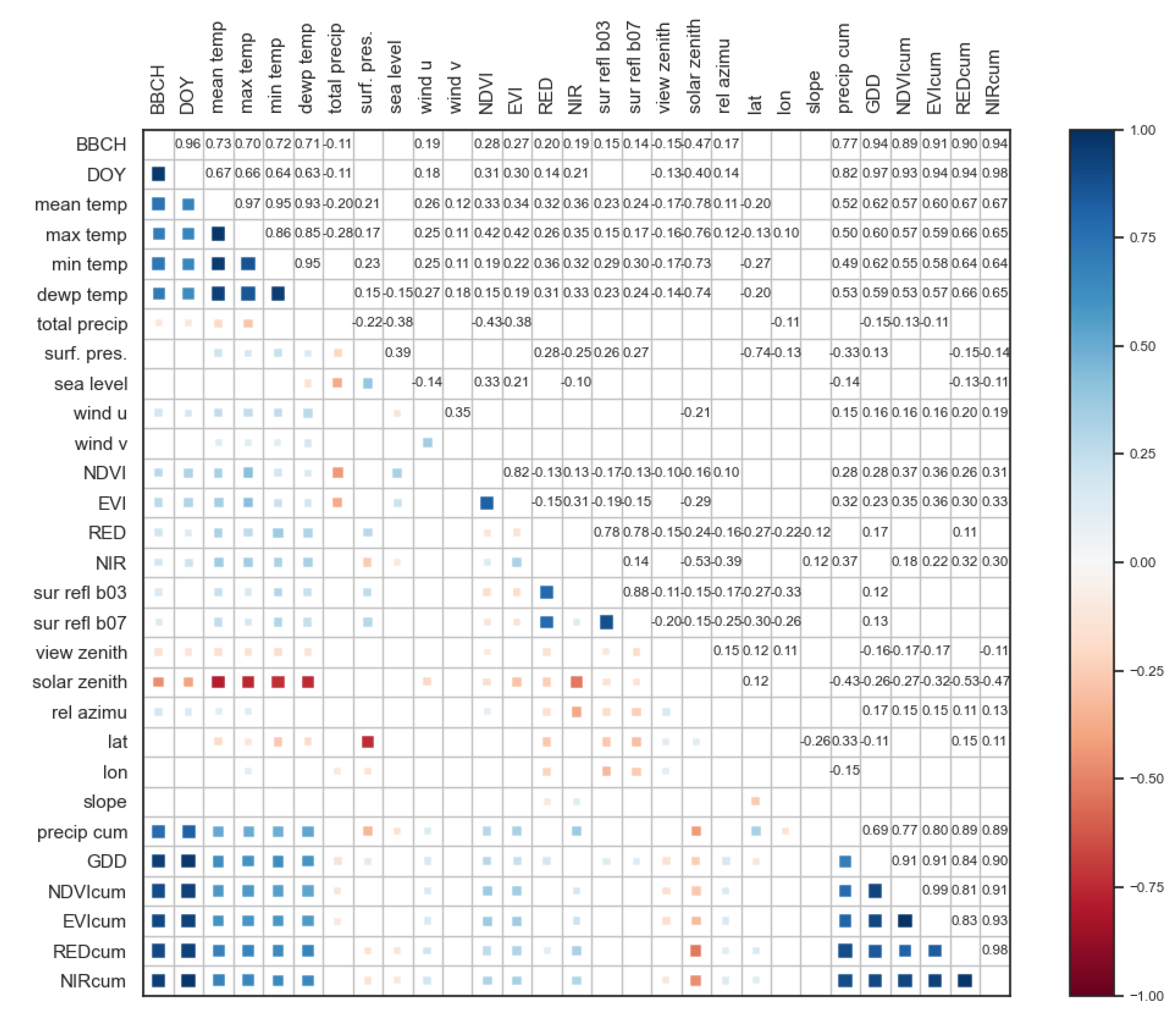
Appendix A. Correlation Matrix
Appendix B. Gephi Configuration and Metrics
Appendix B.1. Layout Configuration Parameters
| Fruchterman Reingold | M1 | M2 |
|---|---|---|
| area | 10 × 10 | 10 × 10 |
| Gravity | 10 | 10 |
| Speed | 1 | 1 |
| Force Atlas Parameters | M1 | M2 |
|---|---|---|
| Inertia | ||
| Repulsion strength | 2 × 10+5 | 200 |
| Attraction strength | 10 | 1 |
| Maximum displacement | 10 | 10 |
| Auto stabilize function | True | True |
| Autostab Strength | 80 | 800 |
| Autostab sensibility | ||
| Gravity | 1 | 1 |
| Attraction Distrib. | True | True |
| Adjust by Sizes | True | False |
| Speed | 1 | 1 |
Appendix B.2. Centrality Metrics
| Label | Degree | Weighted Degree | Modularity Class | Pageranks |
|---|---|---|---|---|
| precip cum | 26 | 353,741 | 0 | 0.08 |
| max temp | 26 | 152,735 | 0 | 0.04 |
| lat | 26 | 174367 | 0 | 0.04 |
| EVIcum | 26 | 148,232 | 0 | 0.04 |
| sur refl b03 | 26 | 123,661 | 0 | 0.03 |
| NIRcum | 26 | 116,685 | 0 | 0.03 |
| dewp temp | 26 | 144,798 | 0 | 0.04 |
| sea level | 26 | 149,325 | 0 | 0.04 |
| slope | 26 | 268,762 | 0 | 0.06 |
| min temp | 26 | 169,226 | 0 | 0.04 |
| sur refl b07 | 26 | 118,982 | 0 | 0.03 |
| REDcum | 26 | 129,930 | 0 | 0.03 |
| RED | 26 | 134,682 | 0 | 0.03 |
| NIR | 26 | 123,034 | 0 | 0.03 |
| mean temp | 26 | 146,211 | 0 | 0.04 |
| NDVIcum | 26 | 145,919 | 0 | 0.04 |
| solar zenith | 26 | 126,423 | 0 | 0.03 |
| rel azimu | 26 | 127,205 | 0 | 0.03 |
| surface pressure | 26 | 159,210 | 0 | 0.04 |
| lon | 26 | 141,790 | 0 | 0.04 |
| GDD | 26 | 167,743 | 0 | 0.04 |
| EVI | 26 | 108,710 | 0 | 0.03 |
| NDVI | 26 | 113,647 | 0 | 0.03 |
| wind v | 26 | 129,516 | 0 | 0.03 |
| total precip | 26 | 115,039 | 0 | 0.03 |
| wind u | 26 | 118,379 | 0 | 0.03 |
| view zenith | 26 | 103,406 | 0 | 0.03 |
| Label | Degree | Weighted Degree | Modularity Class | Pageranks |
|---|---|---|---|---|
| precip cum | 26 | 8604 | 0 | 0.16 |
| lat | 25 | 8354 | 1 | 0.15 |
| max temp | 22 | 2694 | 0 | 0.05 |
| sur refl b03 | 21 | 1968 | 0 | 0.04 |
| sea level | 21 | 1904 | 1 | 0.04 |
| slope | 20 | 1542 | 1 | 0.03 |
| RED | 20 | 1444 | 1 | 0.03 |
| NDVIcum | 20 | 1890 | 1 | 0.04 |
| min temp | 19 | 1716 | 1 | 0.03 |
| dewp temp | 18 | 2220 | 1 | 0.04 |
| surface pressure | 17 | 1822 | 2 | 0.04 |
| EVIcum | 17 | 1972 | 0 | 0.04 |
| solar zenith | 17 | 2046 | 2 | 0.04 |
| REDcum | 17 | 1992 | 1 | 0.04 |
| mean temp | 17 | 2032 | 2 | 0.04 |
| NIR | 16 | 840 | 0 | 0.02 |
| lon | 15 | 1276 | 0 | 0.03 |
| sur refl b07 | 15 | 1152 | 1 | 0.02 |
| rel azimu | 14 | 1046 | 1 | 0.02 |
| EVI | 13 | 910 | 1 | 0.02 |
| GDD | 11 | 1030 | 1 | 0.02 |
| NDVI | 9 | 602 | 0 | 0.02 |
| NIRcum | 8 | 402 | 0 | 0.01 |
| wind u | 7 | 338 | 1 | 0.01 |
| total precip | 4 | 126 | 1 | 0.01 |
| view zenith | 2 | 8 | 0 | 0.01 |
| wind v | 1 | 2 | 0 | 0.01 |
Appendix C. Validation Section Extra Info
| Features | Scores |
|---|---|
| GDD | 6806.02 |
| NIRcum | 6383.33 |
| EVIcum | 3927.72 |
| REDcum | 3605.50 |
| NDVIcum | 3264.47 |
| precip cum | 1216.78 |
| mean temp | 962.07 |
| min temp | 887.57 |
| dewp temp | 829.22 |
| max temp | 799.95 |
| solar zenith | 226.54 |
| NDVI | 69.70 |
| EVI | 65.79 |
| RED | 34.90 |
| NIR | 31.40 |
| wind u | 30.94 |
| rel azimu | 25.39 |
| view zenith | 18.10 |
| sur refl b03 | 17.83 |
| sur refl b07 | 16.64 |
| total precip | 9.45 |
| sea level | 4.72 |
| lon | 3.75 |
| lat | 1.90 |
| surf. pres. | 1.07 |
| wind v | 0.28 |
| slope | 0.06 |
| Features | Scores |
|---|---|
| GDD | 1.72 |
| NIRcum | 1.29 |
| EVIcum | 1.27 |
| solar zenith | 1.23 |
| NDVIcum | 1.22 |
| mean temp | 1.11 |
| sea level | 1.04 |
| REDcum | 1.01 |
| dewp temp | 1.00 |
| min temp | 0.93 |
| max temp | 0.93 |
| precip cum | 0.73 |
| total precip | 0.45 |
| wind u | 0.36 |
| surf. pres. | 0.33 |
| wind v | 0.33 |
| rel azimu | 0.28 |
| view zenith | 0.24 |
| NIR | 0.24 |
| NDVI | 0.17 |
| EVI | 0.15 |
| sur refl b07 | 0.11 |
| RED | 0.09 |
| sur refl b03 | 0.08 |
| slope | 0.00 |
| lon | 0.00 |
| lat | 0.00 |
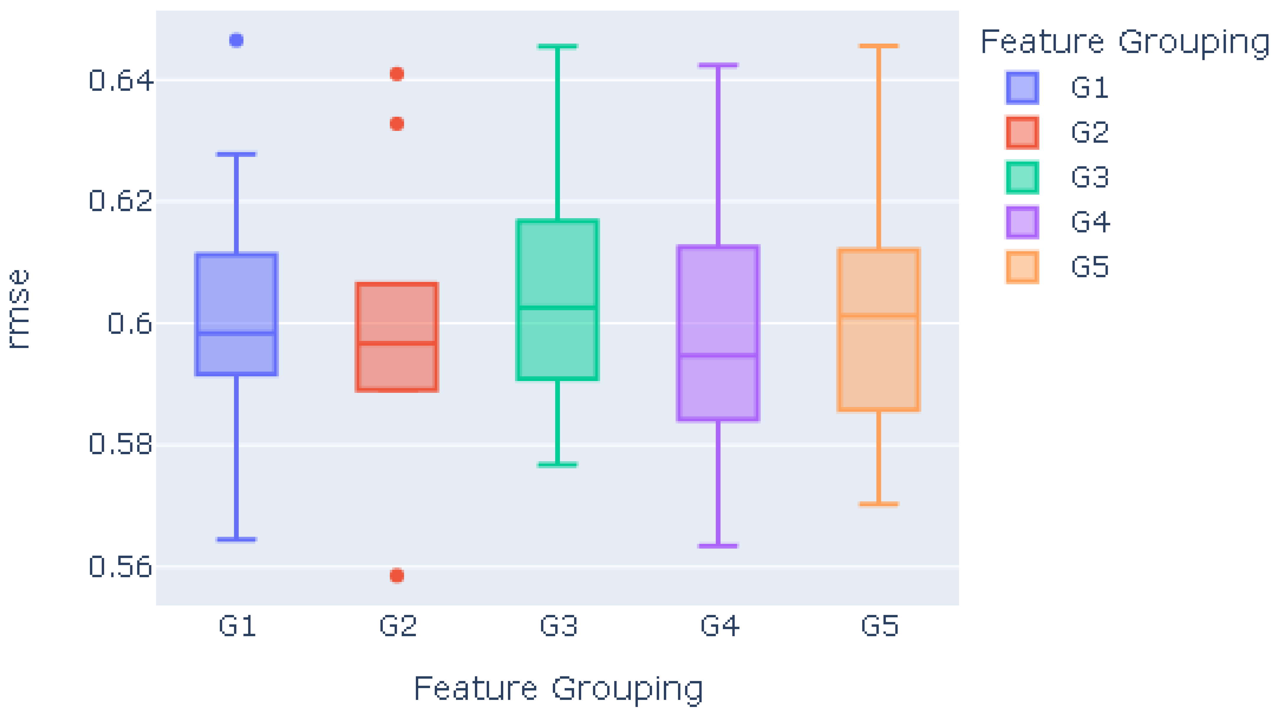
| Feature | RMSE | ||||||
|---|---|---|---|---|---|---|---|
| Grouping | Mean | std | Min | 25% | 50% | 75% | Max |
| G1 | 0.602 | 0.023 | 0.564 | 0.592 | 0.598 | 0.609 | 0.646 |
| G2 | 0.600 | 0.023 | 0.559 | 0.590 | 0.597 | 0.605 | 0.641 |
| G3 | 0.604 | 0.019 | 0.577 | 0.591 | 0.603 | 0.615 | 0.645 |
| G4 | 0.600 | 0.024 | 0.563 | 0.584 | 0.595 | 0.610 | 0.642 |
| G5 | 0.603 | 0.021 | 0.570 | 0.589 | 0.601 | 0.611 | 0.646 |
References
- Chandrashekar, G.; Sahin, F. A survey on feature selection methods. Comput. Electr. Eng. 2014, 40, 16–28. [Google Scholar] [CrossRef]
- Guyon, I.; Elisseeff, A. An introduction to variable and feature selection. J. Mach. Learn. Res. 2003, 3, 1157–1182. [Google Scholar]
- Keogh, E.; Mueen, A. Curse of Dimensionality. In Encyclopedia of Machine Learning and Data Mining; Sammut, C., Webb, G.I., Eds.; Springer: Boston, MA, USA, 2017; pp. 314–315. [Google Scholar]
- Bellman, R. Dynamic programming. Science 1966, 153, 34–37. [Google Scholar] [CrossRef]
- Hasan, B.M.S.; Abdulazeez, A.M. A review of principal component analysis algorithm for dimensionality reduction. J. Soft Comput. Data Min. 2021, 2, 20–30. [Google Scholar]
- Zhou, H.; Wang, F.; Tao, P. t-Distributed stochastic neighbor embedding method with the least information loss for macromolecular simulations. J. Chem. Theory Comput. 2018, 14, 5499–5510. [Google Scholar] [CrossRef]
- Salman, R.; Alzaatreh, A.; Sulieman, H. The stability of different aggregation techniques in ensemble feature selection. J. Big Data 2022, 9, 1–23. [Google Scholar] [CrossRef]
- Duch, W.; Wieczorek, T.; Biesiada, J.; Blachnik, M. Comparison of feature ranking methods based on information entropy. In Proceedings of the 2004 IEEE International Joint Conference on Neural Networks (IEEE Cat. No. 04CH37541), Budapest, Hungary, 25–29 July 2004; Volume 2, pp. 1415–1419. [Google Scholar]
- Breiman, L. Random forests. Mach. Learn. 2001, 45, 5–32. [Google Scholar] [CrossRef]
- Chen, X.W.; Jeong, J.C. Enhanced recursive feature elimination. In Proceedings of the IEEE Sixth International Conference on Machine Learning and Applications (ICMLA 2007), Cincinnati, OH, USA, 13–15 December 2007; pp. 429–435. [Google Scholar]
- Kraskov, A.; Stögbauer, H.; Grassberger, P. Estimating mutual information. Phys. Rev. E 2011, 69, 066138. [Google Scholar] [CrossRef]
- Doshi, M. Correlation based feature selection (CFS) technique to predict student Perfromance. Int. J. Comput. Netw. Commun. 2014, 6, 197. [Google Scholar] [CrossRef]
- Sanderson, C.; Paliwal, K.K. Polynomial features for robust face authentication. In Proceedings of the IEEE International Conference on Image Processing, Rochester, NY, USA, 22–25 September 2002; Volume 3, pp. 997–1000. [Google Scholar]
- Duch, W. Filter methods. In Feature Extraction: Foundations and Applications; Springer: Berlin/Heidelberg, Germany, 2006; pp. 89–117. [Google Scholar]
- Mlambo, N.; Cheruiyot, W.K.; Kimwele, M.W. A survey and comparative study of filter and wrapper feature selection techniques. Int. J. Eng. Sci. (IJES) 2016, 5, 57–67. [Google Scholar]
- Liu, H.; Zhou, M.; Liu, Q. An embedded feature selection method for imbalanced data classification. IEEE/CAA J. Autom. Sin. 2019, 6, 703–715. [Google Scholar] [CrossRef]
- Azpiroz, I.; Oses, N.; Quartulli, M.; Olaizola, I.G.; Guidotti, D.; Marchi, S. Comparison of Climate Reanalysis and Remote-Sensing Data for Predicting Olive Phenology through Machine-Learning Methods. Remote Sens. 2021, 13, 1224. [Google Scholar] [CrossRef]
- Vettoretti, M.; Di Camillo, B. A variable ranking method for machine learning models with correlated features: In-silico validation and application for diabetes prediction. Appl. Sci. 2021, 11, 7740. [Google Scholar] [CrossRef]
- Kotsiantis, S.; Kanellopoulos, D. Association rules mining: A recent overview. GESTS Int. Trans. Comput. Sci. Eng. 2006, 32, 71–82. [Google Scholar]
- Ünvan, Y.A. Market basket analysis with association rules. Commun. Stat. Theory Methods 2021, 50, 1615–1628. [Google Scholar] [CrossRef]
- Annie, L.C.M.; Kumar, A.D. Market basket analysis for a supermarket based on frequent itemset mining. Int. J. Comput. Sci. Issues (IJCSI) 2012, 9, 257. [Google Scholar]
- Kaur, M.; Kang, S. Market Basket Analysis: Identify the changing trends of market data using association rule mining. Procedia Comput. Sci. 2016, 85, 78–85. [Google Scholar] [CrossRef]
- Gayle, S. The Marriage of Market Basket Analysis to Predictive Modeling. In Proceedings of the Web Mining for E-Commerce-Challenges and Opportunities, Boston, MA, USA, 20 August 2000; ACM: Boston, MA, USA, 2000. [Google Scholar]
- Oses, N.; Azpiroz, I.; Marchi, S.; Guidotti, D.; Quartulli, M.; Olaizola, I.G. Analysis of Copernicus’ ERA5 Climate Reanalysis Data as a Replacement for Weather Station Temperature Measurements in Machine Learning Models for Olive Phenology Phase Prediction. Sensors 2020, 20, 6381. [Google Scholar] [CrossRef]
- Piña-Rey, A.; Ribeiro, H.; Fernández-González, M.; Abreu, I.; Rodríguez-Rajo, F.J. Phenological model to predict budbreak and flowering dates of four vitis vinifera L. Cultivars cultivated in DO. Ribeiro (North-West Spain). Plants 2021, 10, 502. [Google Scholar] [CrossRef]
- Geurts, P.; Ernst, D.; Wehenkel, L. Extremely randomized trees. Mach. Learn. 2006, 63, 3–42. [Google Scholar] [CrossRef]
- Raschka, S. MLxtend: Providing machine learning and data science utilities and extensions to Python’s scientific computing stack. J. Open Source Softw. 2018, 3, 638. [Google Scholar] [CrossRef]
- Bastian, M.; Heymann, S.; Jacomy, M. Gephi: An open source software for exploring and manipulating networks. In Proceedings of the International AAAI Conference on Web and Social Media, San Jose, CA, USA, 17–20 May 2009; Volume 3, pp. 361–362. [Google Scholar]
- Page, L.; Brin, S.; Motwani, R.; Winograd, T. The PageRank Citation Ranking: Bringing Order to the Web; Rech Report; Stanford InfoLab: Stanford, CA, USA, 1999; Volume 8090, p. 422. [Google Scholar]
- Blondel, V.D.; Guillaume, J.L.; Lambiotte, R.; Lefebvre, E. Fast unfolding of communities in large networks. J. Stat. Mech. Theory Exp. 2008, 2008, P10008. [Google Scholar] [CrossRef]
- Fruchterman, T.M.; Reingold, E.M. Graph drawing by force-directed placement. Softw. Pract. Exp. 1991, 21, 1129–1164. [Google Scholar] [CrossRef]
- Jacomy, M.; Venturini, T.; Heymann, S.; Bastian, M. ForceAtlas2, a continuous graph layout algorithm for handy network visualization designed for the Gephi software. PLoS ONE 2014, 9, e98679. [Google Scholar] [CrossRef] [PubMed]
- Liu, Y.; Mu, Y.; Chen, K.; Li, Y.; Guo, J. Daily activity feature selection in smart homes based on pearson correlation coefficient. Neural Process. Lett. 2020, 51, 1771–1787. [Google Scholar] [CrossRef]
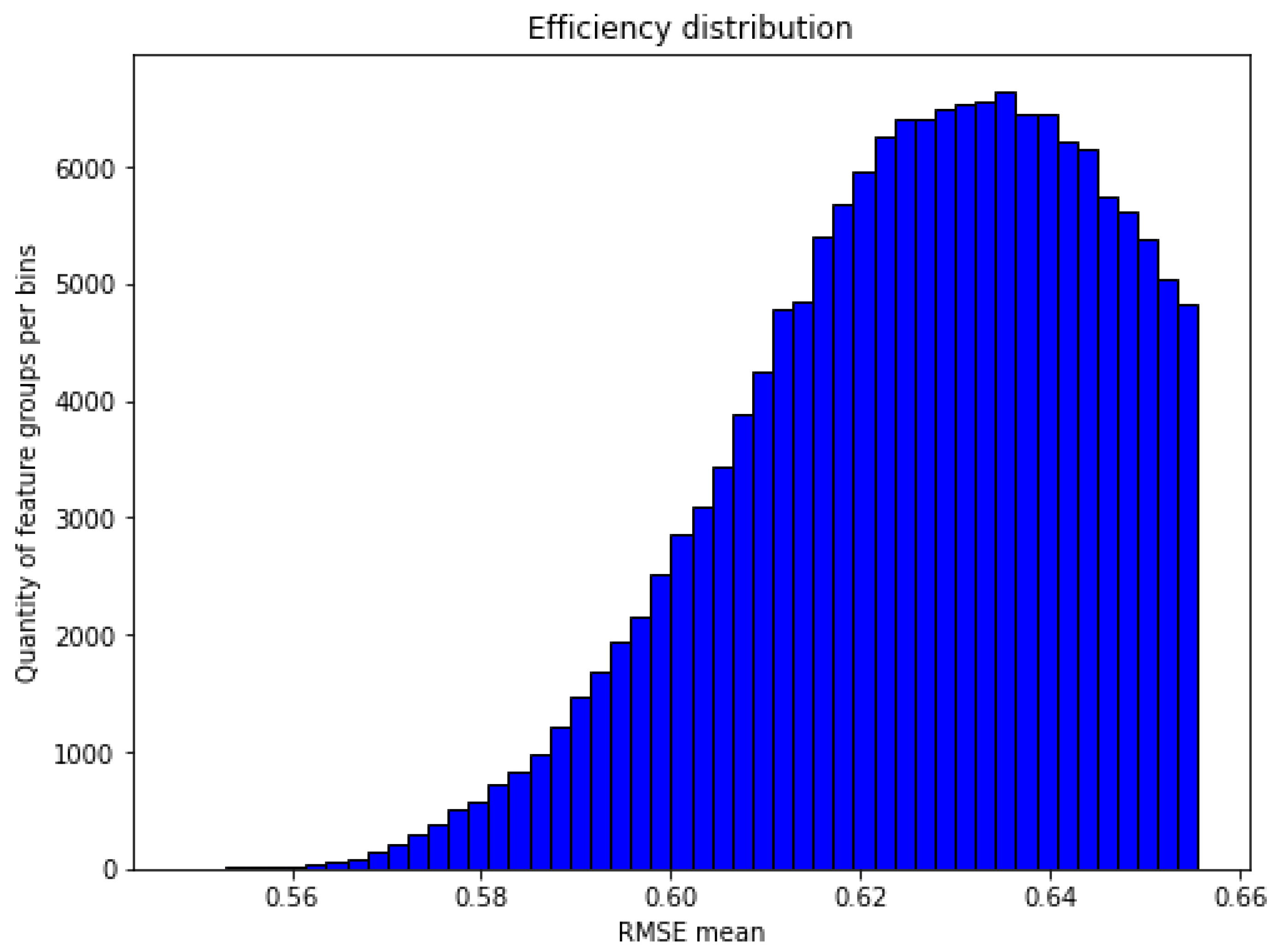


| RMSE | Feature Quantity | |
|---|---|---|
| count | - | 157,135 |
| mean | 0.63 | 6.54 |
| std | 0.02 | 0.63 |
| min | 0.55 | 3 |
| 25% | 0.61 | 6 |
| 50% | 0.63 | 7 |
| 75% | 0.64 | 7 |
| max | 0.66 | 7 |
| Feature | Weight | Feature | Weight | Feature | Weight |
|---|---|---|---|---|---|
| precip cum | 27,053 | mean temp | 8285 | NIR | 4885 |
| lat | 24,946 | sur refl b03 | 7929 | NIRcum | 3960 |
| max temp | 12,051 | dewp temp | 7905 | EVI | 3803 |
| sea level | 11,301 | EVIcum | 7729 | NDVI | 3293 |
| slope | 11,141 | REDcum | 6958 | wind u | 3271 |
| min temp | 10,570 | SolarZenith | 6790 | wind v | 2700 |
| surface pressure | 8699 | lon | 5897 | total precip | 2179 |
| RED | 8602 | sur refl b07 | 5611 | view zenith | 1618 |
| NDVIcum | 8322 | Rel azimuth | 5295 |
| Antecedents | Consequents | a Sup | c Sup | Sup | Conf | Lift | Lev |
|---|---|---|---|---|---|---|---|
| precip cum | lon | 0.47 | 0.20 | 0.10 | 0.20 | 1.02 | 0.00 |
| lon | precip cum | 0.20 | 0.47 | 0.10 | 0.49 | 1.02 | 0.00 |
| lat | slope | 0.25 | 0.35 | 0.09 | 0.37 | 1.03 | 0.00 |
| slope | lat | 0.35 | 0.25 | 0.09 | 0.25 | 1.03 | 0.00 |
| slope | GDD | 0.35 | 0.24 | 0.09 | 0.25 | 1.08 | 0.01 |
| Antecedents | Consequents | a Sup | c Sup | Sup | Conf | Lift | Lev |
|---|---|---|---|---|---|---|---|
| EVIcum | precip cum | 0.21 | 0.52 | 0.11 | 0.54 | 1.03 | 0.00 |
| precip cum | EVIcum | 0.52 | 0.21 | 0.11 | 0.22 | 1.03 | 0.00 |
| lon | precip cum | 0.19 | 0.52 | 0.11 | 0.58 | 1.11 | 0.01 |
| precip cum | lon | 0.52 | 0.19 | 0.11 | 0.22 | 1.11 | 0.01 |
| lat | slope | 0.29 | 0.35 | 0.10 | 0.36 | 1.03 | 0.00 |
| Antecedents | Consequents | a Sup | c Sup | Sup | Conf | Lift | Lev |
|---|---|---|---|---|---|---|---|
| EVIcum | precip cum | 0.21 | 0.57 | 0.13 | 0.63 | 1.09 | 0.01 |
| precip cum | EVIcum | 0.57 | 0.21 | 0.13 | 0.23 | 1.09 | 0.01 |
| lat | slope | 0.37 | 0.34 | 0.13 | 0.34 | 1.03 | 0.00 |
| slope | lat | 0.34 | 0.37 | 0.13 | 0.38 | 1.03 | 0.00 |
| lon | precip cum | 0.19 | 0.57 | 0.13 | 0.67 | 1.17 | 0.02 |
| Antecedents | Consequents | a Sup | c Sup | Sup | Conf | Lift | Lev |
|---|---|---|---|---|---|---|---|
| slope | lat | 0.32 | 0.51 | 0.16 | 0.51 | 1.01 | 0.00 |
| lat | slope | 0.51 | 0.32 | 0.16 | 0.32 | 1.01 | 0.00 |
| EVIcum | precip cum | 0.21 | 0.64 | 0.16 | 0.74 | 1.16 | 0.02 |
| precip cum | EVIcum | 0.64 | 0.21 | 0.16 | 0.25 | 1.16 | 0.02 |
| RED | precip cum | 0.21 | 0.64 | 0.14 | 0.65 | 1.02 | 0.00 |
| Antecedents | Consequents | a Sup | c Sup | Sup | Conf | Lift | Lev |
|---|---|---|---|---|---|---|---|
| max temp | precip cum | 0.32 | 0.71 | 0.23 | 0.73 | 1.02 | 0.00 |
| precip cum | max temp | 0.71 | 0.32 | 0.23 | 0.33 | 1.02 | 0.00 |
| lat | slope | 0.67 | 0.29 | 0.20 | 0.29 | 1.00 | 0.00 |
| slope | lat | 0.29 | 0.67 | 0.20 | 0.67 | 1.00 | 0.00 |
| EVIcum | precip cum | 0.20 | 0.71 | 0.17 | 0.84 | 1.17 | 0.03 |
| Antecedents | Consequents | a Sup | c Sup | Sup | Conf | Lift | Lev |
|---|---|---|---|---|---|---|---|
| precip cum | max temp | 0.88 | 0.36 | 0.33 | 0.37 | 1.05 | 0.02 |
| max temp | precip cum | 0.36 | 0.88 | 0.33 | 0.93 | 1.05 | 0.02 |
| sea level | lat | 0.32 | 0.90 | 0.29 | 0.91 | 1.01 | 0.00 |
| lat | sea level | 0.90 | 0.32 | 0.29 | 0.33 | 1.01 | 0.00 |
| precip cum | max temp, lat | 0.88 | 0.29 | 0.27 | 0.31 | 1.04 | 0.01 |
| max temp, lat | precip cum | 0.29 | 0.88 | 0.27 | 0.92 | 1.04 | 0.01 |
| lat | REDcum | 0.90 | 0.27 | 0.26 | 0.29 | 1.10 | 0.02 |
| REDcum | lat | 0.27 | 0.90 | 0.26 | 0.99 | 1.10 | 0.02 |
| lat | dewp temp | 0.90 | 0.28 | 0.26 | 0.29 | 1.03 | 0.01 |
| dewp temp | lat | 0.28 | 0.90 | 0.26 | 0.92 | 1.03 | 0.01 |
| precip cum | dewp temp | 0.88 | 0.28 | 0.25 | 0.28 | 1.02 | 0.00 |
| dewp temp | precip cum | 0.28 | 0.88 | 0.25 | 0.90 | 1.02 | 0.00 |
| NDVIcum | lat | 0.26 | 0.90 | 0.25 | 0.94 | 1.04 | 0.01 |
| lat | NDVIcum | 0.90 | 0.26 | 0.25 | 0.27 | 1.04 | 0.01 |
| precip cum | REDcum | 0.88 | 0.27 | 0.24 | 0.28 | 1.03 | 0.01 |
Disclaimer/Publisher’s Note: The statements, opinions and data contained in all publications are solely those of the individual author(s) and contributor(s) and not of MDPI and/or the editor(s). MDPI and/or the editor(s) disclaim responsibility for any injury to people or property resulting from any ideas, methods, instructions or products referred to in the content. |
© 2023 by the authors. Licensee MDPI, Basel, Switzerland. This article is an open access article distributed under the terms and conditions of the Creative Commons Attribution (CC BY) license (https://creativecommons.org/licenses/by/4.0/).
Share and Cite
Azpiroz, I.; Quartulli, M.; Olaizola, I.G. Enhancing Olive Phenology Prediction: Leveraging Market Basket Analysis and Weighted Metrics for Optimal Feature Group Selection. Appl. Sci. 2023, 13, 10987. https://doi.org/10.3390/app131910987
Azpiroz I, Quartulli M, Olaizola IG. Enhancing Olive Phenology Prediction: Leveraging Market Basket Analysis and Weighted Metrics for Optimal Feature Group Selection. Applied Sciences. 2023; 13(19):10987. https://doi.org/10.3390/app131910987
Chicago/Turabian StyleAzpiroz, Izar, Marco Quartulli, and Igor G. Olaizola. 2023. "Enhancing Olive Phenology Prediction: Leveraging Market Basket Analysis and Weighted Metrics for Optimal Feature Group Selection" Applied Sciences 13, no. 19: 10987. https://doi.org/10.3390/app131910987
APA StyleAzpiroz, I., Quartulli, M., & Olaizola, I. G. (2023). Enhancing Olive Phenology Prediction: Leveraging Market Basket Analysis and Weighted Metrics for Optimal Feature Group Selection. Applied Sciences, 13(19), 10987. https://doi.org/10.3390/app131910987