Abstract
This research introduces an innovative technique for estimating the particle size distribution of muckpiles, a determinant significantly affecting the efficiency of mining operations. By employing deep learning and simulation methodologies, this study enhances the precision and efficiency of these vital estimations. Utilizing photogrammetry from multi-view images, the 3D point cloud of a muckpile is meticulously reconstructed. Following this, the particle size distribution is estimated through deep learning methods. The point cloud is partitioned into various segments, and each segment’s distinguishing features are carefully extracted. A shared multilayer perceptron processes these features, outputting scores that, when consolidated, provide a comprehensive estimation of the particle size distribution. Addressing the prevalent issue of limited training data, this study utilizes simulation to generate muckpiles and consequently fabricates an expansive dataset. This dataset comprises 3D point clouds and corresponding particle size distributions. The combination of simulation and deep learning not only improves the accuracy of particle size distribution estimation but also significantly enhances the efficiency, thereby contributing substantially to mining operations.
1. Introduction
Blasting is a process of breaking rock mass using explosives, such as in mining, and the resulting pile of broken rock is called muckpile fragmentation. The main purpose of blasting is to break rocks into suitable sizes without damaging surrounding objects and to extract resources contained in the rocks [1]. Blasting is a very effective method of crushing various types of rocks with different hardness in mining, as it can crush a large amount of rocks at once and at a low cost. In addition, muckpile fragmentation is represented by particle size distribution, which is an important parameter for optimizing blasting plans [2].
Currently, methods for measuring the particle size distribution of muckpile fragmentation include sieving and using laser scanners [3], and methods using 2D images [4]. However, sieving requires a tremendous amount of effort to be performed on site, as the amount of rocks that can be measured at once is limited. The cost and knowledge required for laser scanners pose problems when used on site. Therefore, WipFrag [4] (https://wipware.com/products/wipfrag-image-analysis-software/, accessed on 4 September 2023), a method for quickly measuring particle size distribution by processing 2D images, has become more common. However, this method, which is based on 2D images, has been criticized for its low accuracy due to its inability to recognize the complex shapes of rocks [5]. Recent studies have underscored the pivotal role of blast charge initiation techniques in optimizing fragmentation outcomes and ensuring environmental safety, as evidenced by comprehensive analyses using the WipFrag software [6].
To overcome the shortcomings of 2D image-based measurement systems, Tungol et al. [7] reconstructed 3D point clouds from multi-view images of muckpile fragmentation using 3D photogrammetry. They then divided the 3D point clouds into individual rocks using Supervoxel clustering and estimated the particle size distribution by calculating the particle size. However, since the rocks and clusters did not correspond one-to-one, the accuracy of the particle size distribution estimation was insufficient.
Therefore, this study develops a method for quickly and accurately estimating the particle size distribution of muckpile fragmentation using deep learning with simulations and 3D point clouds. By using simulations, which excel at handling 3D models, a large amount of learning data can be obtained without the need for extensive effort in capturing multi-view images on site or measuring particle size distribution by sieving. Instead, a large number of muckpile fragmentation instances with known particle size distributions can be generated and used for deep learning.
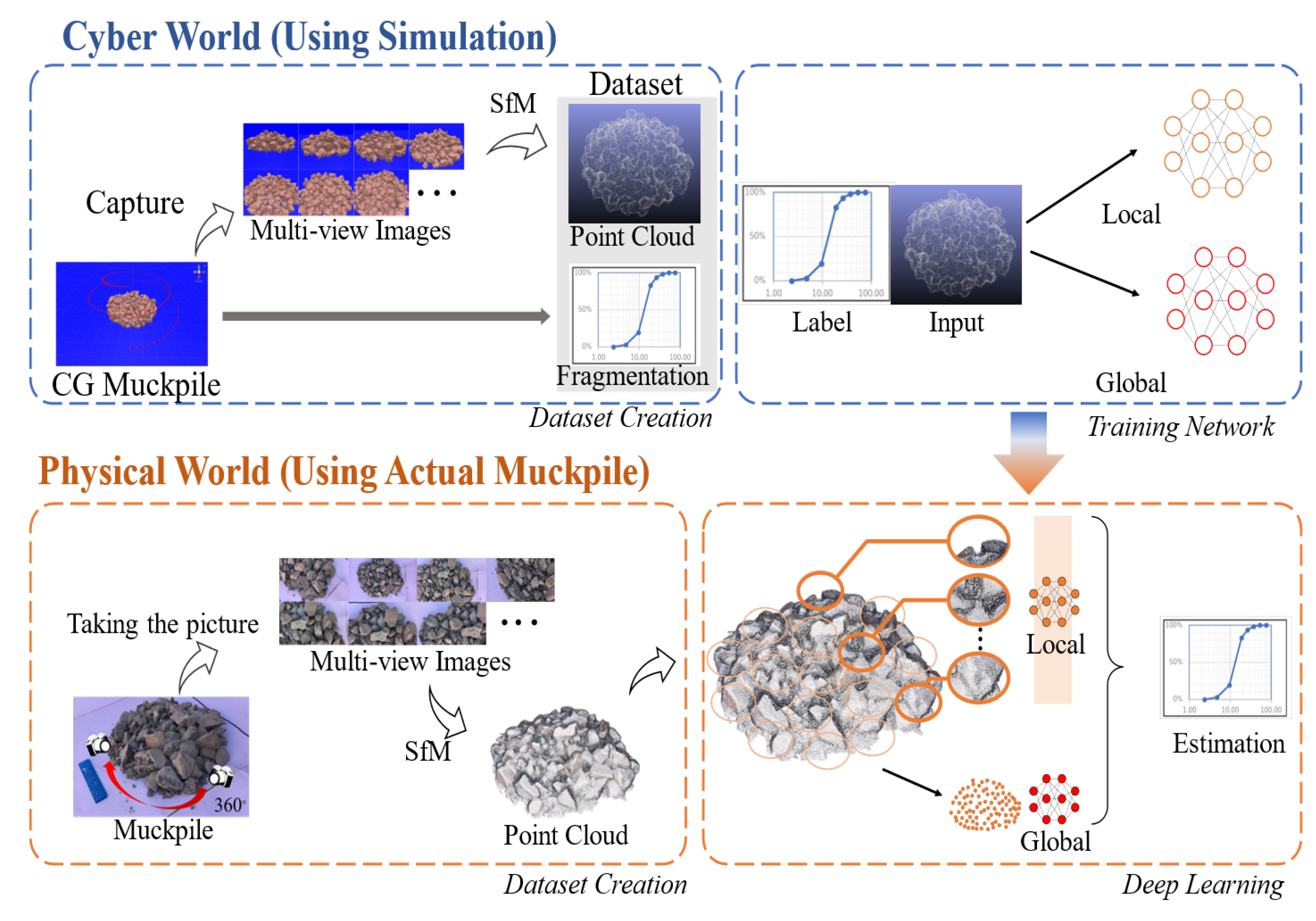
The overall flow of the muckpile fragmentation particle size distribution estimation system in this study is shown in Figure 1. First, the muckpile fragmentation CG model generated by simulation in the Cyber world, the 3D point clouds generated by 3D photogrammetry from multi-view images, and the ground truth particle size distribution are used as learning data for training the particle size distribution estimation network, similar to the method of Tungol et al. [7]. Then, in the Physical world, the 3D point cloud data of actual muckpile fragmentation, reconstructed from multi-view images in the same way as in the Cyber world, is input into the trained particle size distribution estimation network to perform the estimation.
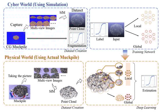
Figure 1.
Proposed System Workflow.
2. Related Work
2.1. Estimation for the Particle Size Distribution
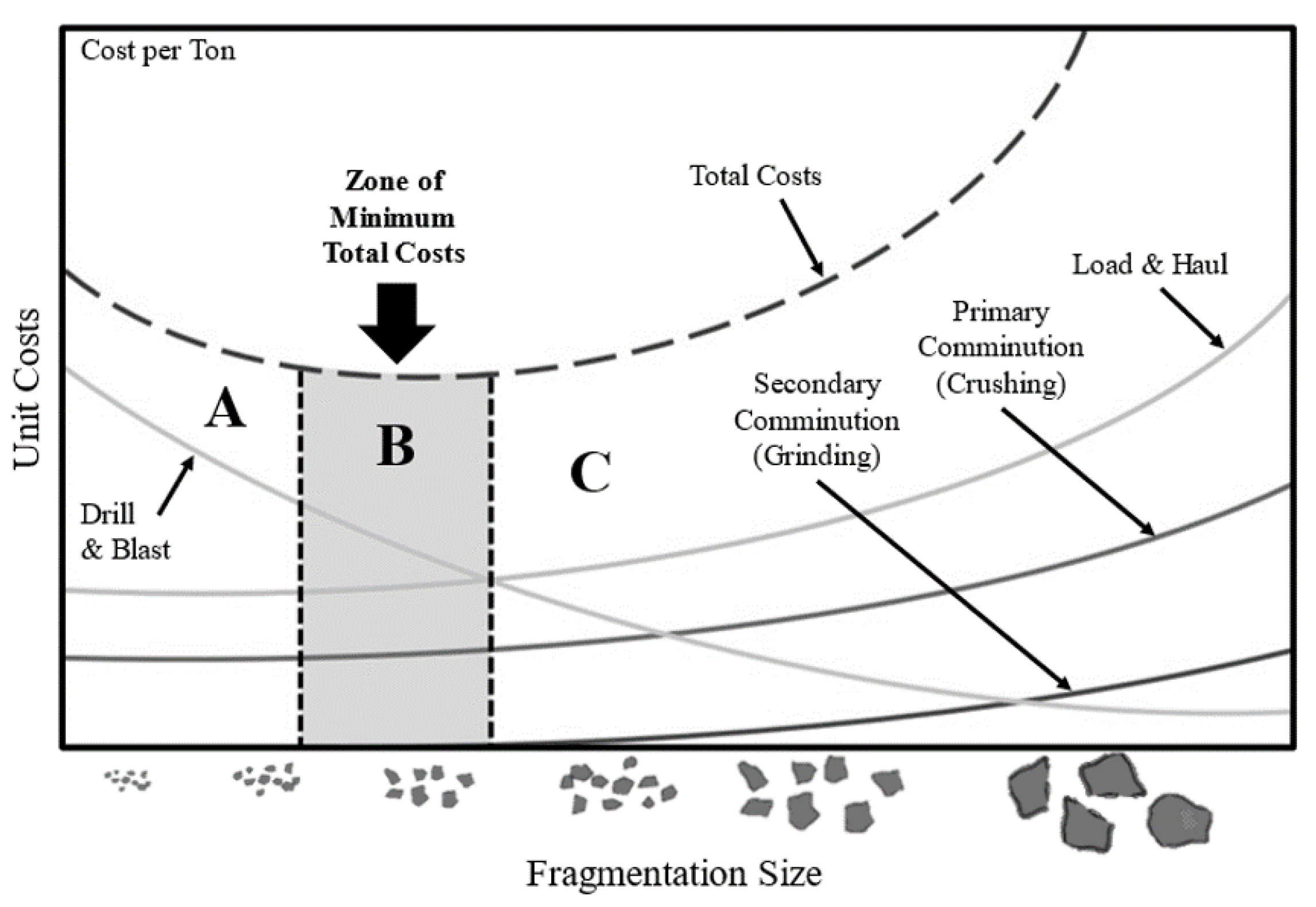
The particle size distribution of blast muckpile has a significant impact on all downstream processes in the mining industry, including loading, hauling, and processing. Figure 2 illustrates the relationship between fragmentation size and unit cost, with the x-axis representing the fragmentation size and the y-axis representing the unit cost. If the fragmentation distribution is skewed towards smaller particles (part A), as shown in Figure 2, useful minerals become excessively fine, resulting in increased costs. Conversely, if the particle size distribution is skewed towards larger particles (part C), transportation becomes challenging and additional mechanical crushing is required after blasting, leading to unnecessary costs. To minimize total costs, blasting should be conducted in a manner that achieves an optimal particle size distribution (aiming at part B). However, controlling blasting is complex, as it depends on various factors such as the amount and type of explosives, the number and depth of blasting holes, and the timing of blasting. Consequently, accurate estimation of the particle size distribution of blast muckpile is essential for optimizing downstream processes, prompting researchers to propose various mathematical models for this purpose, such as the Kuz-Ram mathematical model presented by Cunningham [8], the Swebrec model proposed by Sanchidrian et al. [9], and the Hybrid model introduced by Gheibie et al. [10].
where, B: burden (m), S: spacing (m), D: hole diameter (mm), W: standard deviation of drilling precision (m), L: charge length (m), : bottom charge length (m), : column charge length (m), H: bench height (m).

Figure 2.
Relationship between Fragmentation Size and Operational Costs in Mining.
The Kuz-Ram mathematical model is a common mathematical model for predicting the size distribution of rock fragments caused by blasting. It is widely used in the mining industry because of the ease of collecting input data and the simplicity of the relationship between blasting design and rock fragmentation results. However, one limitation of this predictive mathematical model is that it tends to underestimate the number of fines produced by the blast, which means it cannot be considered a perfect estimation model. The distinction between 2D and 3D imaging in fragmentation estimation lies in the spatial information captured. 3D imagery, with its depth and volume metrics, provides a comprehensive representation of muckpile fragments. Our model is specifically designed to leverage this depth of information inherent in 3D data, allowing for a refined fragmentation estimation process. In the diagram illustrating the relationship between fragmentation size and operational costs in mining, depicted in Figure 2, three zones labeled A, B, and C are shown. In zone A, excessive fragmentation leads to increased costs due to the heightened need for drilling and blasting. Conversely, in zone C, while costs for drilling and blasting are diminished, there is a substantial rise in the subsequent transportation and additional crushing expenses. Zone B stands as the optimal middle ground, highlighting the zone of minimum total costs. Here, both the preliminary and subsequent costs converge to provide the most economical mining operation.
2.2. Estimation Methods Using 2D Images
The rapid advancement of image analysis technology has enabled the development of methods for estimating particle size distribution using image analysis. WipFrag, for instance, is a system that estimates the particle size distribution of blast muckpile using digital image analysis and videotape images [4]. Despite its ease of use and widespread application in mining sites, several drawbacks have been identified with this estimation method. The automatic contouring tool built into the 2D image processing system requires manual correction, making it less user-friendly. This process can be time-consuming and prone to human error, leading to potential inaccuracies in the estimated particle size distribution [11]. Additionally, the quality of the input images has a significant impact on the accuracy of the estimation. Factors such as lighting conditions, camera angle, and image resolution can all influence the reliability of the results [12].
Furthermore, estimating the particle size distribution of the entire blast muckpile necessitates the analysis of multiple moving photographs, each requiring calibration. The process of calibrating multiple images can be cumbersome, and the complexity increases with the number of images involved [13]. The overlapping nature of blast muckpile and the potential for particles to be too small for recognition can lead to overestimation of particle size distribution [14]. In an effort to address these limitations, researchers have proposed alternative methods, such as those based on stereoscopic imaging and 3D reconstruction [2,15]. These approaches aim to improve the accuracy of particle size distribution estimation by leveraging the additional depth information provided by multiple images or 3D models. However, these methods can also be more computationally intensive and may require specialized equipment, potentially limiting their widespread adoption in the mining industry.
2.3. Estimation Using 3D Images
Recent advancements in muckpile fragmentation estimation have shifted from traditional 2D imaging systems to more advanced 3D model-based techniques [16,17]. Our proposed approach harnesses the power of Structure-from-Motion (SfM), a state-of-the-art 3D photogrammetry method [2,18], combined with Patch-based Multi-View Stereo (PMVS) [4,19]. This methodology allows for the detailed reconstruction of muckpile’s 3D shape, subsequently facilitating the estimation of its particle size distribution.
The resulting 3D structure is portrayed as a point cloud, where each point represents a specific position in space. To discern individual rocks within the muckpile, we employed the Supervoxel clustering technique. This method clusters these points based on the k-means objective function [20,21], taking into account parameters like Euclidean distance, color differentiation, and normal vectors. By applying the Laplacian of Gaussian filter to multi-view images of the muckpile, we can effectively detect rock edges [22].
The process further categorizes clusters based on specific thresholds. When a point surpasses a predetermined boundary threshold between two clusters, these clusters are distinguished as separate rocks. Conversely, if no points exceed this threshold, clusters are identified as the same rock, merging them. A significant challenge arises here, as the number of clusters doesn’t always equate to the actual number of rocks. This disparity complicates the precise measurement of particle size distribution, especially when aiming to consolidate multiple clusters representing a single rock.
One approach to addressing the challenge of accurately measuring the particle size distribution is to use a combination of machine learning techniques, such as deep learning and convolutional neural networks (CNNs), to improve the detection and segmentation of rocks within the 3D point cloud [23,24]. These methods have been successfully applied in various fields, including object recognition, image segmentation, and 3D point cloud processing. By training a model with a large dataset of labeled 3D point clouds, the deep learning algorithms can learn to identify and segment rocks more accurately, potentially improving the estimation of the particle size distribution.
Another possibility is to integrate other sources of information, such as LiDAR data, to enhance the accuracy of the 3D models and the subsequent particle size distribution estimation [25,26]. By combining different types of data, more accurate and robust models can be generated, leading to improved estimations of the particle size distribution and better optimization of downstream processes in the mining industry. In an effort to provide a comprehensive evaluation of our method, a comparative analysis with conventional estimation techniques has been included. This juxtaposition not only validates the performance of our proposed method but also elucidates its relative strengths.
3. Methodology
3.1. Photogrammetry
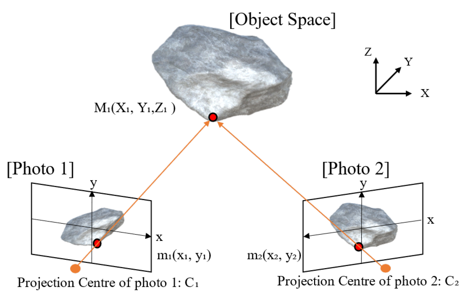
Photogrammetry is a technology that simultaneously recovers the position and orientation of the camera and the 3D shape of an object from multi-view images of the object taken from various angles using SfM [27]. This technology makes it possible to efficiently photograph and reconstruct the 3D shape of blast muckpile. In recent years, the availability of affordable and high-resolution digital cameras, along with the increased computational power of personal computers, has significantly improved the potential of photogrammetry for various applications [28]. The process of 3D photogrammetry consists of several stages, as shown in Figure 3, where the 3D shape is constructed by transforming the 2D image coordinates of several photographs into 3D coordinates . First, the images are preprocessed, which involves the removal of lens distortion and the normalization of image brightness and contrast [29]. Next, a feature matching process is performed, in which distinctive points in the images are identified and matched across multiple images. The matched features are then used to estimate the camera’s pose and calibrate the camera [30]. Drawing from recent research on the effectiveness of ANN in predicting blast impacts, it’s crucial to adapt their methodologies to address current gaps in our study [31].
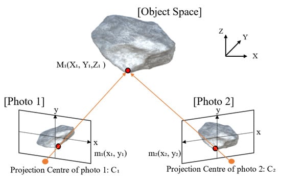
Figure 3.
Example of Photogrammetric System.
Once the camera calibration is complete, a sparse 3D reconstruction is generated using SfM. This initial reconstruction is often too sparse for many applications, so a denser reconstruction is obtained using PMVS [19,32]. Finally, a mesh model is created from the dense point cloud, and a texture is applied to the mesh to generate a realistic 3D model [33]. In this study, we used Agisoft Metashape, a 3D modeling software, which can extract feature points from multiple 2D photographs of a surveyed object using SfM and reconstruct a dense 3D point cloud from a sparse point cloud using PMVS [34]. It is also possible to reconstruct textures and place scales. The software offers various tools for processing and analyzing the reconstructed 3D model, such as tools for measuring distances, areas, and volumes, as well as for exporting the model to various formats [34]. While recognizing that the foundational system model has been discussed in prior works, this study introduces a novel integration of cloud data capabilities with deep learning algorithms for muckpile fragmentation estimation. Our approach aims to harness the expansive potential of cloud data to further enhance the efficiency and accuracy of fragmentation analysis.
3.2. Deep Learning
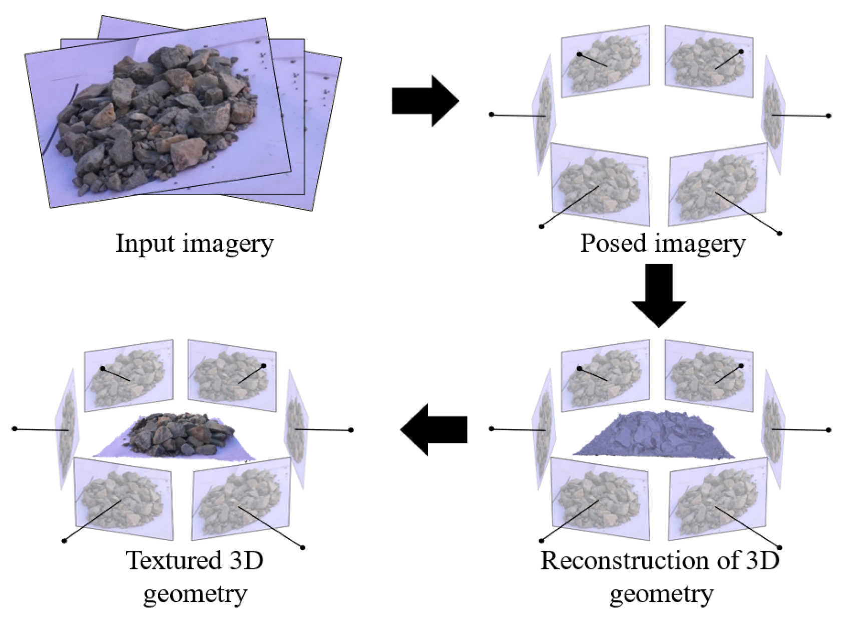
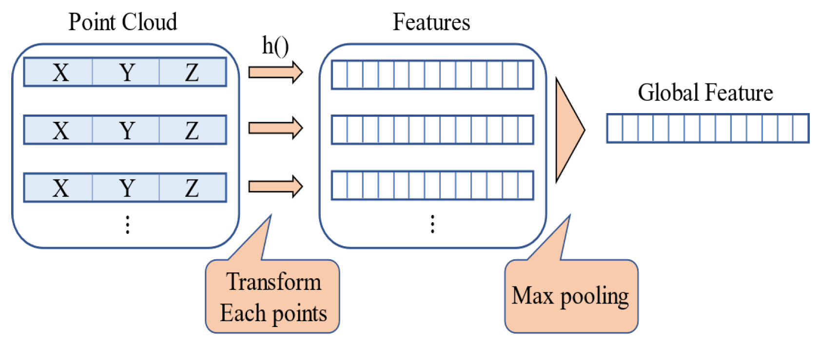
Deep learning is a subset of machine learning that employs neural networks to learn complex patterns and representations from large datasets. One of the challenges in applying deep learning to 3D point cloud data is that point clouds are simply unordered sets of points, lacking the regular structure found in images or voxel grids [35]. This structure difference, when compared to the regular grid pattern seen in the example of the Multi-view Stereo Pipeline illustrated in Figure 4, makes point clouds particularly challenging. PointNet is a pioneering deep learning method designed to work directly with 3D point cloud data as input [36]. While voxel grids and images have traditionally been the preferred data formats for deep learning, PointNet can effectively perform classification and segmentation tasks on unordered 3D point cloud data. When dealing with point clouds, several issues need to be addressed, such as the unordered nature of the points and the invariance to geometric transformations. To tackle the issue of unordered points, PointNet employs a symmetric function, which is invariant to the order of the input points. As illustrated in Figure 5, each point is independently transformed and processed before a max-pooling operation is applied to extract global features of the point cloud without depending on the order of the points.

Figure 4.
Example of Multi-view Stereo Pipeline.

Figure 5.
Using Logarithmic Functions.
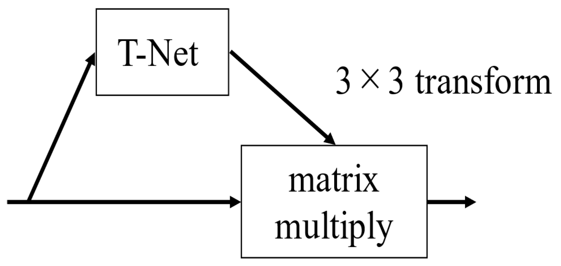
In addition to order invariance, point clouds also exhibit transformation invariance. A point cloud representing the same shape can have different positions and orientations but should be recognized as the same object. To address this issue, PointNet introduces a subnetwork called T-Net, shown in Figure 6. The T-Net estimates an affine transformation matrix that aligns the input point cloud to a canonical space, thus providing approximate invariance to translations and rotations [36]. This paper leverages the classification capabilities of PointNet to analyze blast muckpile. The proposed approach involves preprocessing the point cloud data to ensure that it is suitable for PointNet, followed by training the neural network on a labeled dataset of muckpile. The trained network can then be used to classify and segment new muckpile data, enabling the estimation of particle size distributions and other relevant properties. Several studies have demonstrated the effectiveness of PointNet in various applications, such as object recognition, scene understanding, and semantic segmentation of point clouds [24,35,37].

Figure 6.
T-Net Functions.
3.3. Experimental Procedures
In this study, we propose a method to estimate the particle size distribution of muckpile using an improved PointNet network, which is a deep learning technique that reconstructs the 3D point cloud of muckpile and acquires features from local shapes. This method consists of two phases: the learning phase and the inference phase. In the learning phase, simulation is used to create training data. The processing flow is shown in Figure 7. After generating the CG model of the muckpile using the simulation, multi-view images are obtained with a virtual camera, and point cloud data is obtained using SfM. In addition, the true particle size distribution is measured and used as the dataset for training the particle size distribution estimation. Since we are using a CG model of rocks with known sizes in this study, it is possible to measure the particle size distribution of the muckpile CG model. After training the particle size distribution estimation network using this dataset, in the inference phase, the actual muckpile is photographed and point cloud reconstruction is performed. The particle size distribution is then estimated by inputting the reconstructed point cloud into the trained network.
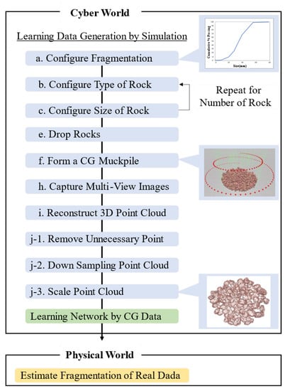
Figure 7.
Flow of the Experiment.
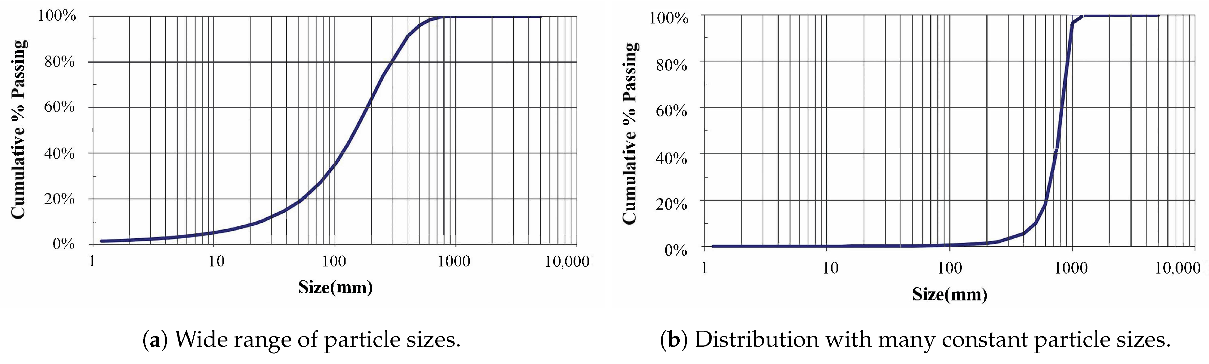
The particle size distribution of muckpile is represented by the cumulative distribution shown in Figure 8, with the vertical axis being the cumulative undersize value and the horizontal axis being the particle size. The cumulative undersize distribution is independent of the interval setting, unlike the frequency distribution, so anyone can obtain the same distribution when tallying the data. Moreover, the proportion of particle sizes is represented by the slope of the graph. In the case of Figure 8a, the gentle slope indicates the presence of particles with a wide range of sizes. On the other hand, Figure 8b shows that particles around 800 mm are most abundant due to the steep slope. In the mining field, it is important for the particle size distribution of muckpile to have a certain particle size, as shown in Figure 8c.
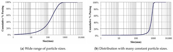
Figure 8.
Example of Particle-size Distribution.
4. Simulation-Based Learning Data Generation
4.1. Creation of Muckpile CG Model
The generation of the muckpile CG model was carried out using simulation. As shown in Figure 7, a large number of muckpile CG models were generated by automatically repeating these procedures:
- (a)
- Configure Fragmentation
- (b)
- Configure Type of Rock
- (c)
- Configure Size of Rock
- (d)
- Placing the rocks in mid-air in the simulation
- (e)
- Drop Rocks
- (f)
- Form a CG Muckpile
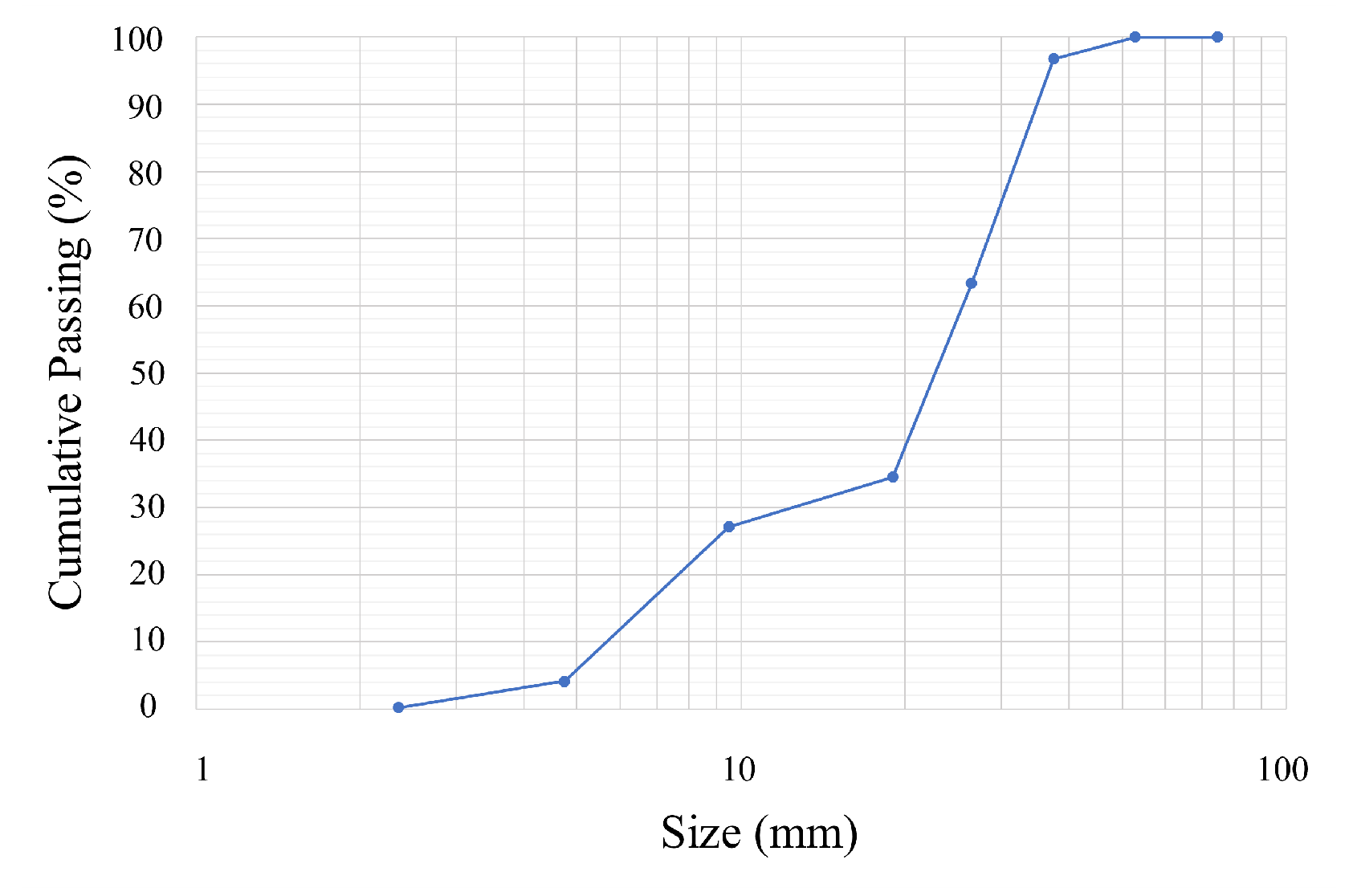
In step (a), the particle size distribution of the muckpile CG model to be generated was set as shown in Figure 9. Here, the particle size distribution was changed randomly within the range of [2.36, 4.76, 9.5, 19, 26.5, 37.5, 53, 75] (mm) from 0 mm to 80 mm in 8 stages, allowing the generation of muckpile with various particle size distributions.
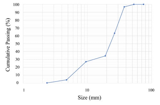
Figure 9.
Particle Size Distribution of CG Muckpile.
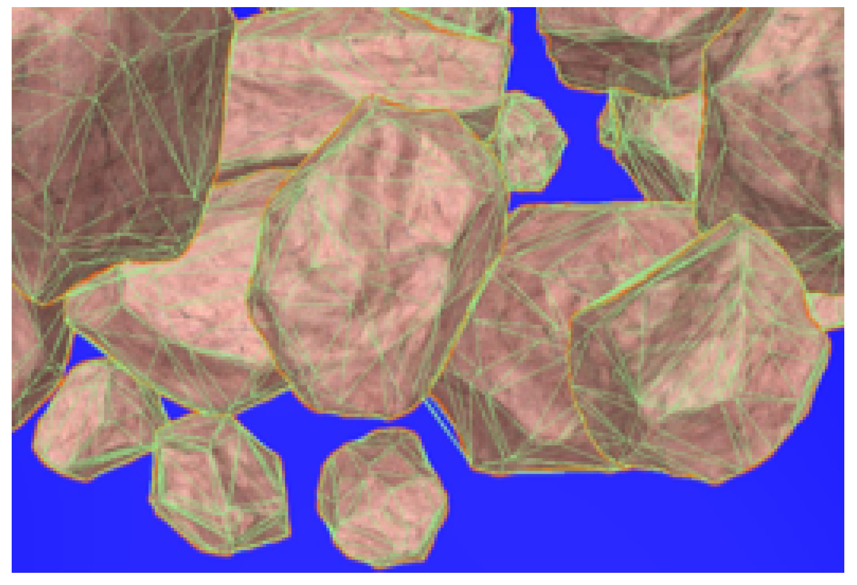
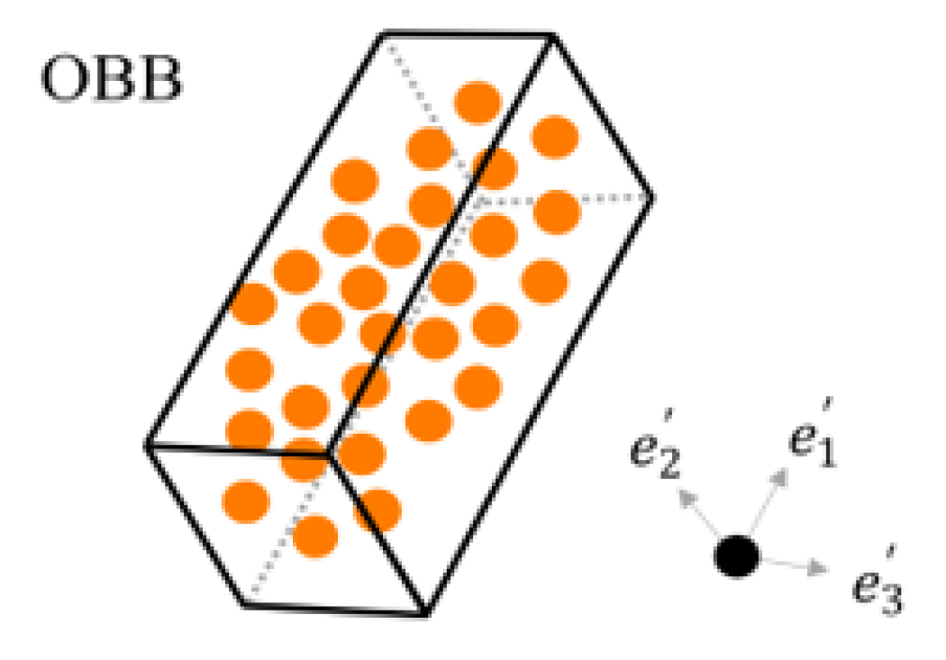
Next, in step (b), a rock CG model was randomly selected from 18 different shaped rock CG models, and in step (c), the rocks were scaled according to the 8-stage particle size distribution set in step (a) ranging from 0 mm to 80 mm, [2.36, 4.76, 9.5, 19, 26.5, 37.5, 53, 75] (mm). In order to generate a more faithful muckpile CG model, actual rock CG models obtained by 3D scanning were used for the rocks, and mesh division was performed on the rocks by vertices, edges, and faces to accurately perform scaling of rock sizes and collision detection during free fall. Figure 10 shows a rock CG model with mesh division, which is divided into multiple polygons. The particle size of the rock CG model was determined by the length when a Bounding-Box was applied. The Bounding-Box used the values calculated by Oriented Bounding-Box as the particle size, as shown in Figure 11. First, the 3D covariance matrix was calculated from the mesh vertex coordinates of the rock CG model, and the eigenvalues were calculated. When the eigenvectors are sorted in descending order of eigenvalues as , , and , they become the first, second, and third principal components, respectively, and form an orthonormal basis. The Bounding-Box is set with these axes. The length is determined by calculating the difference between the vertex with the maximum value and the vertex with the minimum value for each axis. Considering the situation in which a rock passes through the sieve mesh in measurements using a sieve, the size of the second axis was used as the particle size of the rock 3D CG model.

Figure 10.
Segmentation by Mesh.

Figure 11.
OBB: Oriented Bounding-Box.
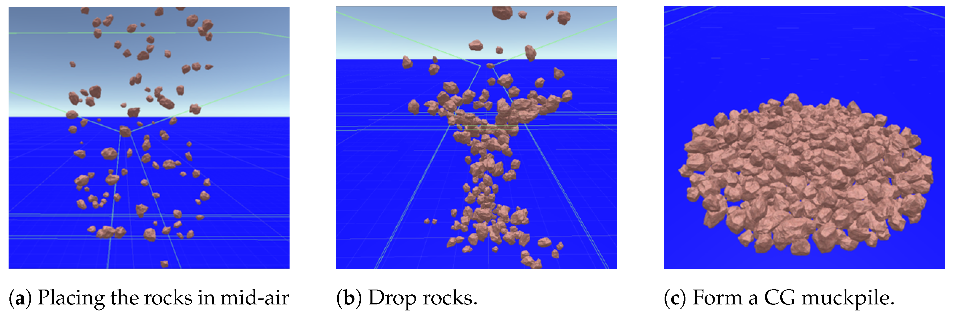
After that, by repeating steps (b) and (c), a large number of rock groups were generated, and in step (d), the rocks were placed in mid-air in the simulation, and in step (e), the rocks were freely dropped to form the muckpile CG model. The process of rock CG models accumulating and forming the muckpile CG model is shown in Figure 12. Figure 12a shows the rock CG models being generated in mid-air. The green-framed board shown here is a board that repels when a rock CG model collides with it, and four slanted boards and a cylindrical board were placed to accumulate the rock CG models around the center. In Figure 12b, the falling rock CG models are shown forming the muckpile CG model while colliding with the board. In this way, the formation of the muckpile CG model as shown in Figure 12c was performed.
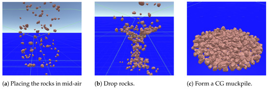
Figure 12.
Creating a Computer-Generated Muckpile.
In addition, when dropping the rock CG models, the physical calculations based on the parameters shown in Table 1 were applied. Dynamic Friction is the friction coefficient for moving objects, and Static Friction represents the friction coefficient used for stationary objects. Both of these friction coefficients were set to 0.9 in order to make all the rock CG models used in this experiment accumulate. These two friction coefficients are used with values ranging from 0 to 1. In the case of 0, the object does not stop, like on ice, and in the case of 1, the object does not move unless a strong force or gravity is applied to it. Bounciness indicates how much elasticity is on the surface, and in this experiment, the purpose was to accumulate, so it was set to 0.1. Friction Combine and Bounciness Combine represent the friction coefficient and bounce level of colliding objects, respectively, and were set to Average.

Table 1.
Parameter of the Simulation.
4.2. Creating Point Cloud Data
The point cloud data of the muckpile CG model was generated using the muckpile CG model created in Section 4.1. The procedure is as follows:
- (g)
- Placement of Virtual Cameras Around the Muckpile CG Model
- (h)
- Capture Multi-View Images
- (i)
- Reconstruct 3D Point Cloud
- (j)
- Point Cloud Preprocessing:
- (j-1)
- Remove Unnecessary Point
- (j-2)
- Down Sampling of Point Cloud
- (j-3)
- Scale Point Cloud
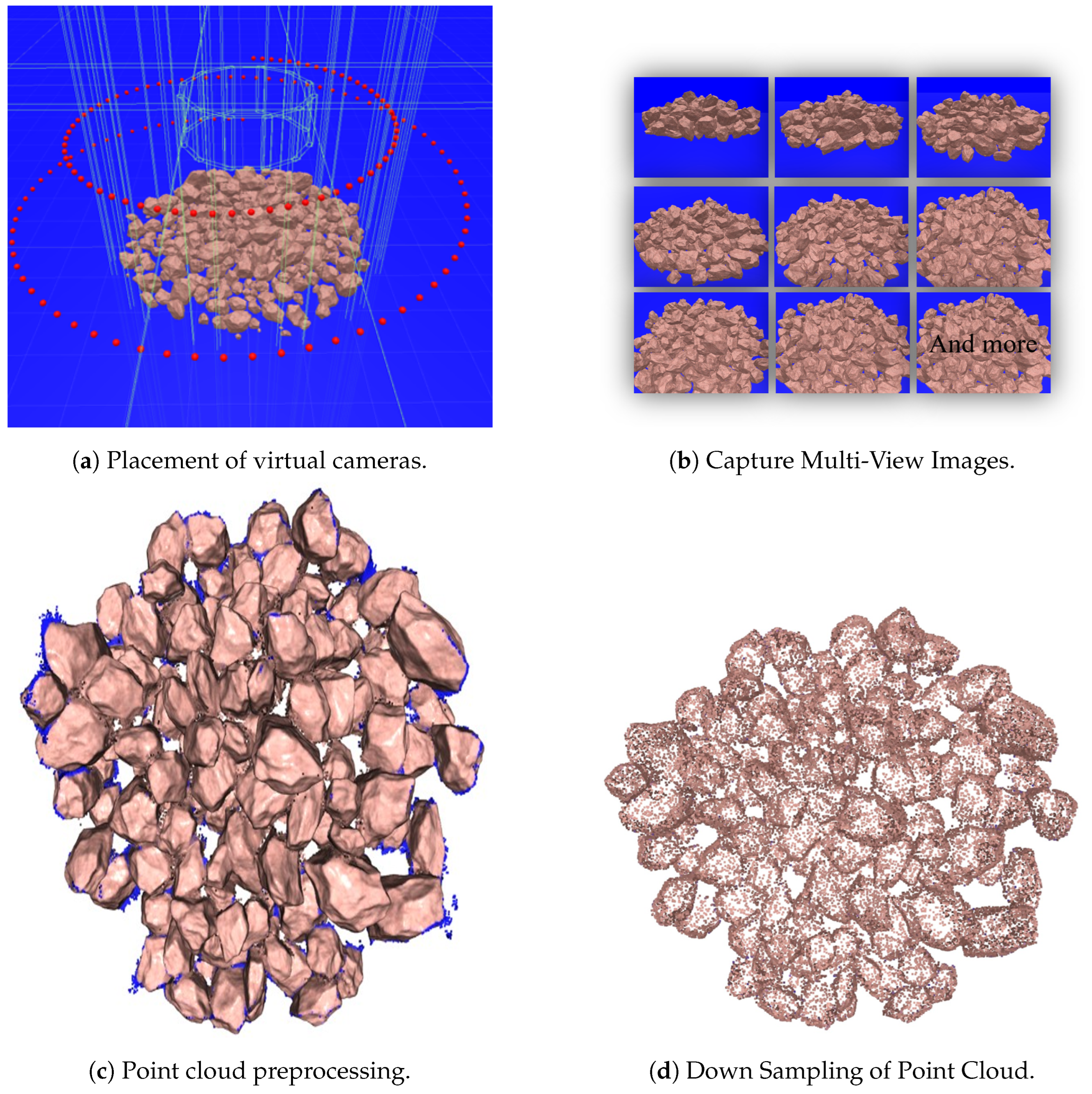
In step (g), as shown in Figure 13a, virtual cameras were placed around the muckpile CG model accumulated in the simulation in a spiral pattern covering 360 degrees. The red spherical object indicates the placement of the virtual cameras. Next, in step (h), 144 multi-view images, as shown in Figure 13b, were obtained by rendering the muckpile CG model at 1024 × 768 pixels from the placed virtual cameras. In step (i), the 3D point cloud reconstruction, as shown in Figure 13c, was performed by applying SfM. At this time, the green-framed wall used for generating the muckpile CG model exists as a transparent wall in the simulation and is not included in the rendered images. Therefore, it is not shown in the acquired multi-view images. Subsequently, preprocessing for deep learning was performed in step (j), Figure 13d. In step (j-1), blue point removal was carried out to reduce errors, as not only the muckpile CG model but also the background color, etc., are reconstructed simultaneously during the 3D point cloud reconstruction. Blue points are the simulation background color reconstructed as a 3D point cloud, and in this simulation, the blue color ([R G B] = [0 0 255]) is significantly different from the color information of the rock CG model used for generating the muckpile CG model. Therefore, this background color was selected and removed. In step (j-2), downsampling was performed from approximately 300,000 points to 50,000 points for the purpose of data reduction when applying deep learning. Finally, in step (j-3), the point cloud of the muckpile CG model reconstructed by SfM may slightly change in scale, so scaling was performed to reduce errors by making all point clouds fit within a sphere of radius 1. Through these steps, the 3D point cloud reconstruction of the muckpile CG model was performed, and these data were used as training data.
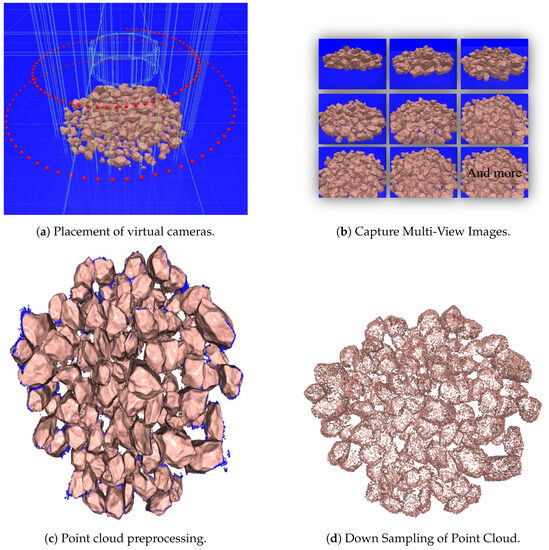
Figure 13.
Steps in Generating and Processing Multi-View Point Clouds.
5. Verification of Particle Size Distribution Estimation
5.1. Particle Size Distribution Estimation Network
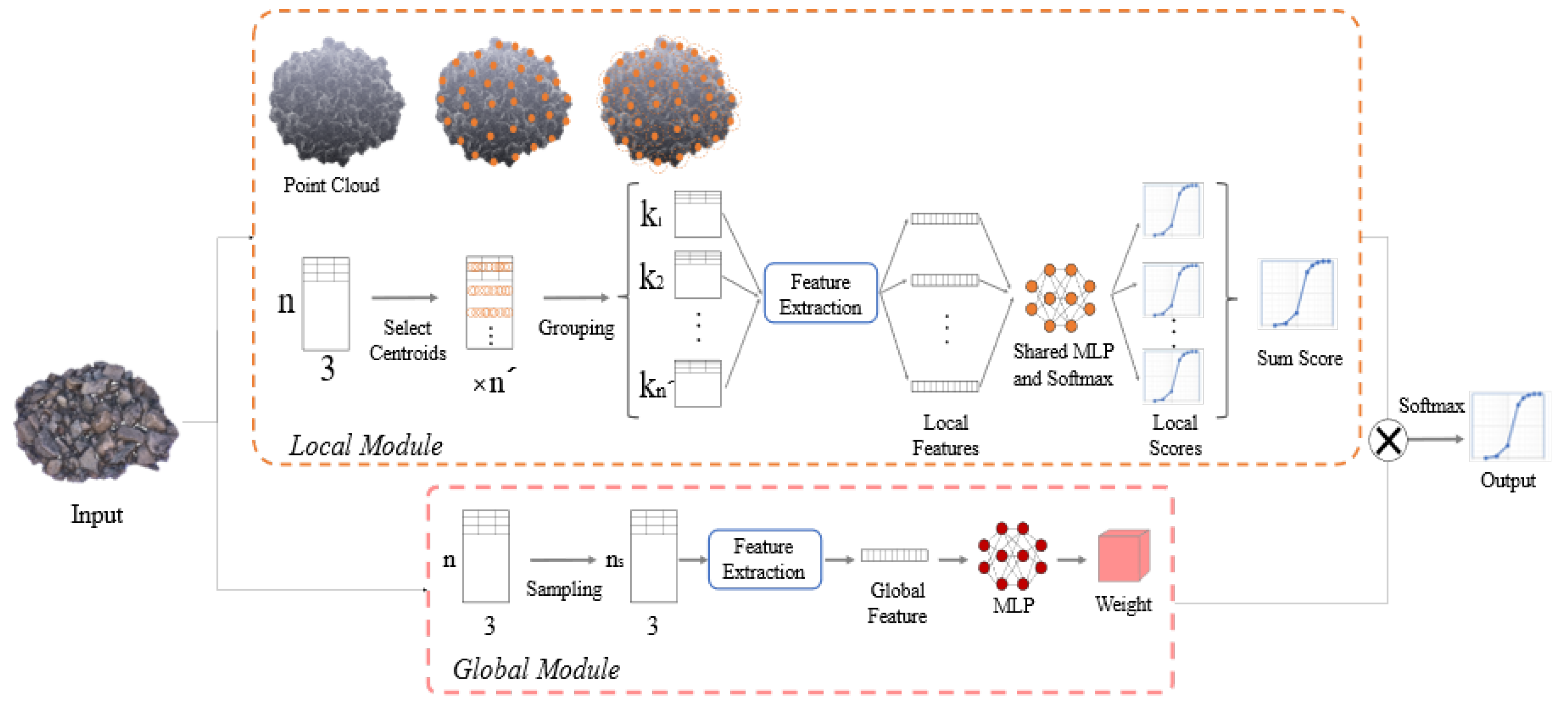
The particle size distribution estimation network used in this study is a modified version of PointNet++ [37], which is an advanced version of PointNet [35]. PointNet++ [37] is proposed as a method to capture local features by hierarchically applying PointNet to each group of divided point clouds. In this experiment, we used a modified version of PointNet++ for particle size distribution estimation. The network structure is shown in Figure 14. The network consists of a Local Module and a Global Module. The Local Module divides the point cloud into multiple groups using a sphere with radius r. It captures features, learns from all points in each group as a single PointSet, and calculates a score. The Global Module captures global shape features from the sampled point cloud and multiplies them with the final score of the Local Module as weights.
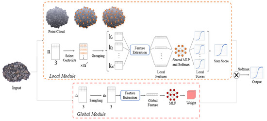
Figure 14.
Architecture of Fragmentation Estimation Network.
The Local Module takes the XYZ coordinates of the 3D point cloud as input and selects centroids for group division using FPS (FPS: Farthest Point Sampling). In FPS, a point is selected randomly, and this point becomes the first centroid. The second centroid is the point farthest from the first, and the third centroid is the point farthest from the first and second. This is repeated to select centroids up to the n’th. By using FPS, it is possible to sample points spatially evenly. In this study, the points selected as centroids are limited to the range from the “center of the point cloud” to “r inside the edge” so that local shape patterns can be learned appropriately. Furthermore, by setting the radius r so that the largest rock in the data fits into a sphere, appropriate learning can be achieved. After generating n’ groups, feature extraction is performed for each group as shown in Figure 5. After feature extraction, a Shered MLP is applied to each feature. This MLP is shared within the group, learned to output a score from the shape of the group, and finally normalized by the Softmax function to sum up the scores.
The Global Module takes the XYZ coordinates of the 3D point cloud as input and samples points using FPS. Feature extraction is performed on the sampled point cloud as shown in Figure 4, and the overall feature is output. Then, an MLP is applied to generate weights. The score output from the Local Module is multiplied by the weight obtained from the Global Module and normalized by the Softmax function to obtain the final output. When the particle size distribution is at the d-stage, the output is a d-dimensional discrete probability distribution.
In addition, the Kullback-Leibler divergence was used as the loss function for the difference between the output d-dimensional discrete probability distribution and the correct label, which is the particle size distribution. Let the output vector be and the correct particle size distribution be . The loss function is represented by Equation (2).
To estimate the particle size distribution, the Bhattacharyya Distance (: Bhattacharyya Distance) is used as the evaluation function for the difference between the correct label particle size distribution and the estimated particle size distribution. Let the two distributions be and . It is expressed as in Equation (3).
5.2. Particle Size Distribution Estimation Using CG Data
Using the training data created in Section 4, the particle size distribution estimation network was trained. For the training, 1000 sets of data consisting of 3D point cloud data and corresponding particle size distribution data as labels were used. Out of the 1000 sets, 800 were used for training, 100 for validation, and 100 for testing. The computer used was the supercomputer Cygnus [38] at the University of Tsukuba’s Center for Computational Sciences, equipped with a CPU: Intel Xeon Gold 6126 Processor and four GPU: NVIDIA Tesla V100 32GiB. The batch size for training was 16, the initial learning rate was , the parameter update was done using the Adam method [39], and the training was conducted for 2000 epochs. At this time, the radius r of the sphere when generating groups in the Local module was set to 0.15 so that the largest rock in the simulation would fit. During training, the point cloud data was randomly and slightly rotated and the points were slightly shifted for data augmentation.
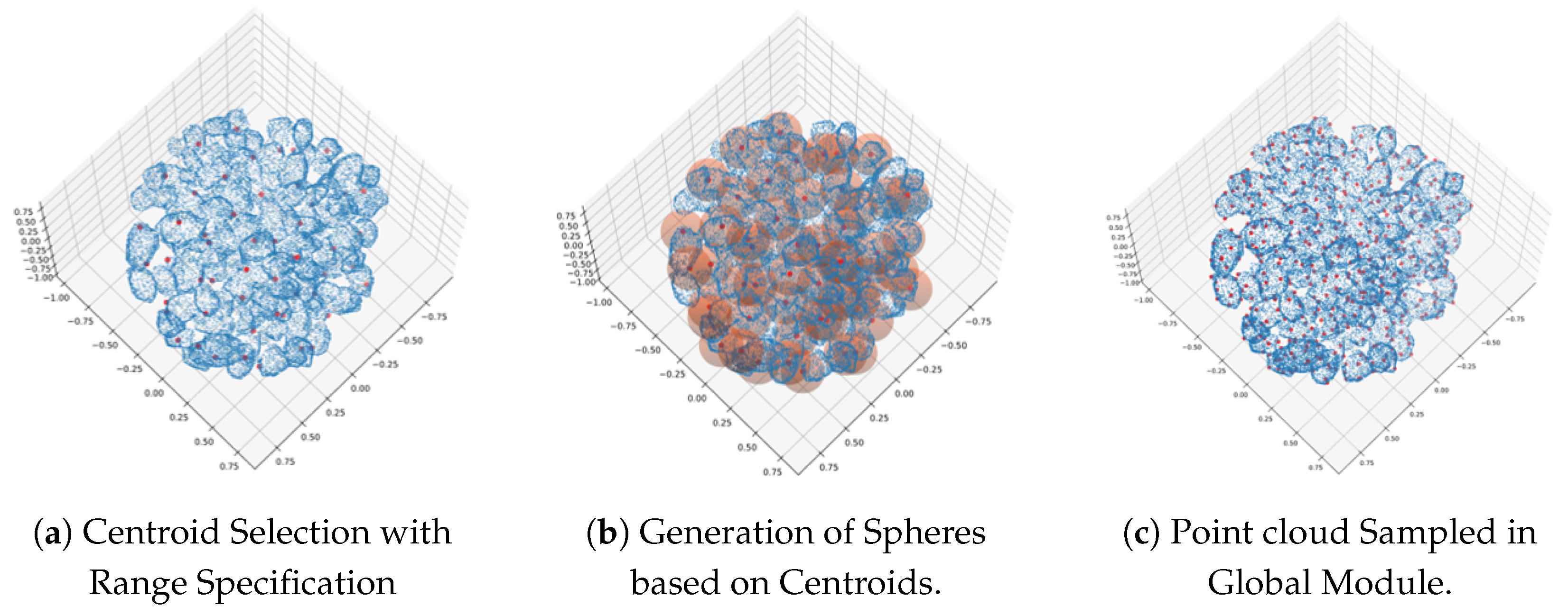
The results of performing group division using the FPS method with the input 3D point cloud XYZ coordinates are shown in Figure 15. Figure 15a,b show the results of group division in the Local module. The blue point cloud in Figure 15a represents the input XYZ coordinates of the muckpile fragmentation, and the red points indicate the selected centroids. Figure 15b shows the result of generating spheres with radius r centered on the selected centroids. From these results, it was confirmed that each centroid was spatially sampled evenly. In addition, Figure 15c shows the result of sampling in the Global module. The sampled point cloud retains the overall shape information of the muckpile fragmentation rather than the fine shape information. From these results, it was confirmed that the sampling in the Global module was also performed appropriately.

Figure 15.
Results of group partitioning using Farthest Point Sampling.
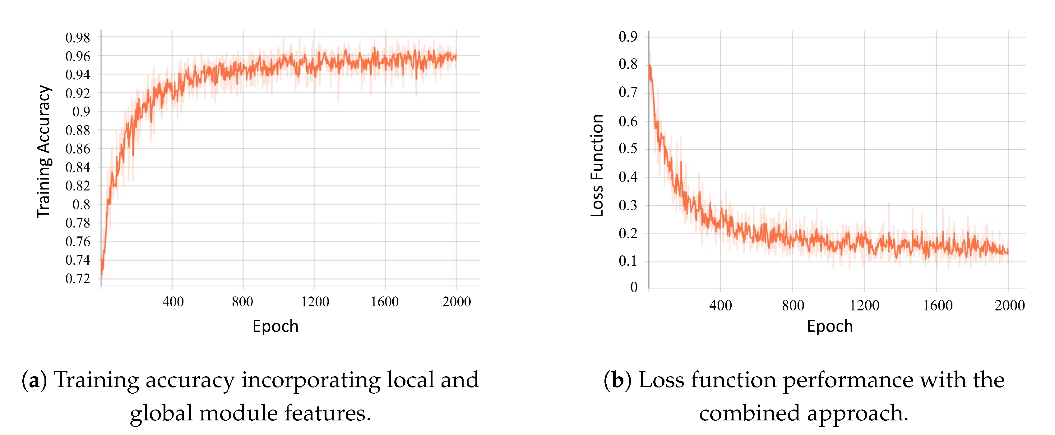
The results of adding the features learned in the Global module to the particle size distribution scores obtained in the Local module and performing the training are shown in Figure 16. As shown in Figure 16a, the learning curve depicts an accuracy of 96.3% during the training phase. Figure 16b illustrates the transition of the loss function, which evaluates the magnitude of the difference between the estimated values and the correct values; the value of the loss function was recorded as 0.1237. It is essential to note that the stated 96.3% accuracy pertains specifically to the training data. We will further provide the exact estimation accuracy in subsequent sections to offer a comprehensive view of the model’s overall performance. The results underline that the muckpile fragmentation particle size distribution estimation network utilized in this study demonstrates efficacy with the simulation-generated training data.
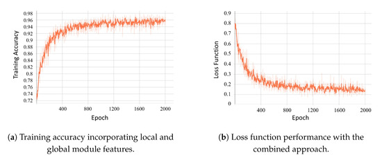
Figure 16.
Performance evaluation of the combined approach using local and global module features.
5.3. Particle Size Distribution Estimation Using Actual Data
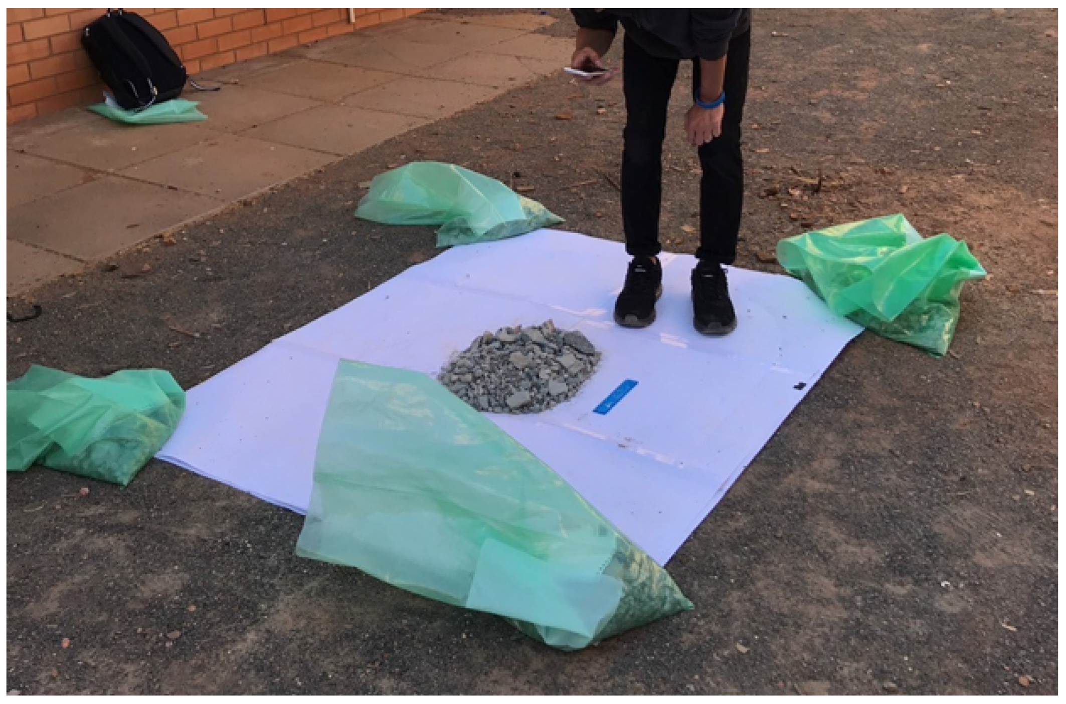
Using the model trained in Section 5.2, the particle size distribution estimation was performed on actual data in the Physical world. For the actual data, three sample data of muckpile fragmentation measured at Curtin University in Kalgoorlie, Australia, were used. The sample data of muckpile fragmentation consisted of particle size distributions measured by sieving at eight levels of [2.36, 4.76, 9.5, 19, 26.5, 37.5, 53, 75] (mm), and as shown in Figure 17, the multi-view images captured by the camera were reconstructed into 3D point clouds using SfM, similar to the Cyber world. An iPhone 6s was used as the camera, and the image resolution was 1080 pixels by 1929 pixels. The reconstructed point clouds were preprocessed by background point removal, downsampling to 50,000 points, and scaling, and then input into the trained model in the Cyber world for estimation.

Figure 17.
The experiment of taking multi-view photos.
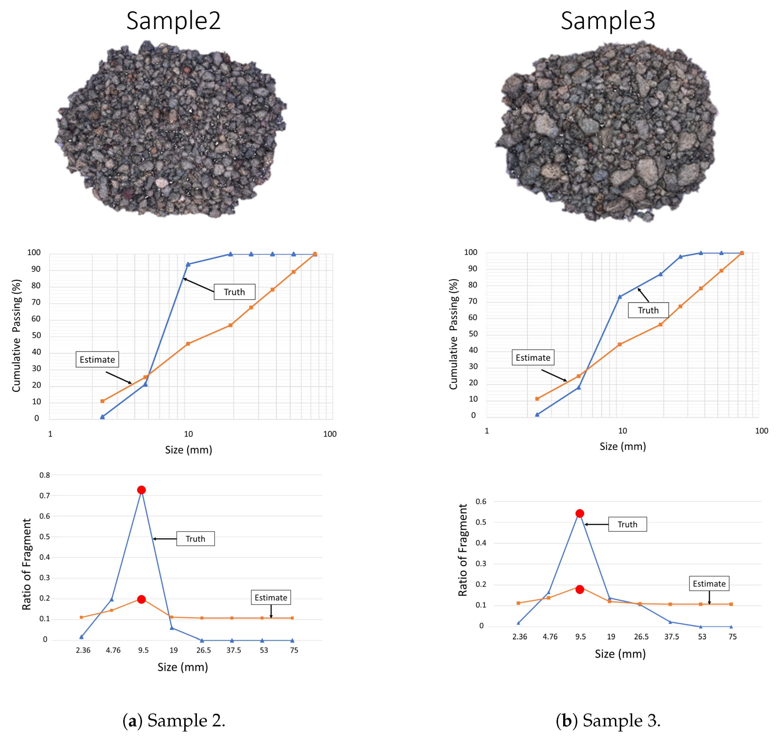
Figure 18 shows the results of the particle size distribution estimation for muckpile fragmentation sample 1. Figure 18 represents the cumulative undersize distribution, with the blue line indicating the actual distribution and the yellow line indicating the estimated values. From these results, although the estimation results recognized about 10% of the rocks at [2.36, 53, 75] (mm) which were not included in the actual data, a generally close particle size distribution could be estimated. Next, the results for muckpile fragmentation samples 2 (Figure 19a) and 3 (Figure 19b) are shown in Figure 19. The upper graph represents the cumulative undersize distribution, and the lower graph represents the proportion of each of the eight particle sizes contained in the muckpile fragmentation, with the blue line indicating the actual values and the yellow line indicating the estimated values. From these results, the cumulative undersize distributions for samples 2 and 3 were significantly different from the actual particle size distributions. However, when the estimated results were compared in terms of the proportions of each particle size, the distribution peaks for samples 2 and 3 matched, and a close overall shape of the distribution could be obtained. However, in muckpile fragmentation like sample 2, which does not contain rocks smaller than 2.36 mm and larger than 26.5 mm, the estimation should be zero, but the estimation was still performed. Factors that may be affecting the estimation results include overlapping ranges when generating groups in the Local module and areas not included in the group.
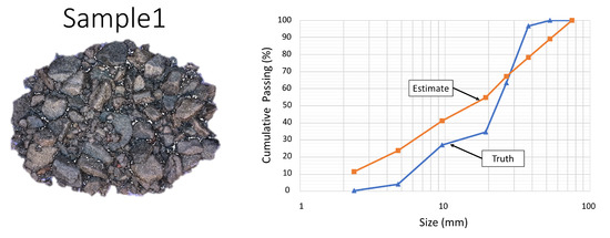
Figure 18.
Estimation Results of Particle Size Distribution for Sample 1.
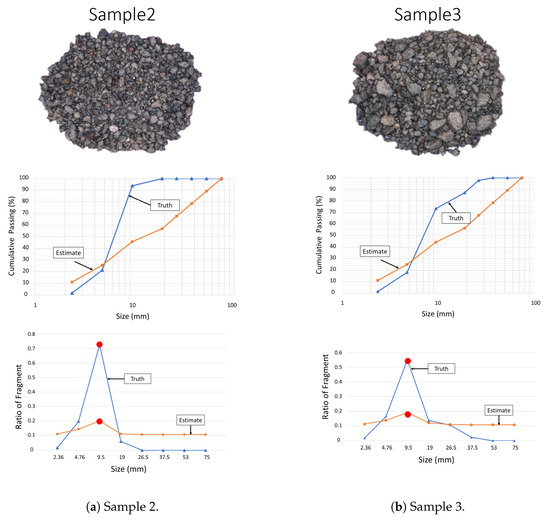
Figure 19.
Estimation Results of Particle Size Distribution.
From these results, it can be said that the particle size distribution estimation network trained and learned in the Cyber world can effectively estimate the particle size distribution of actual muckpile fragmentation.
6. Conclusions
In this study, we presented a novel approach for estimating the particle size distribution of blasted rock fragments (muckpile) by leveraging simulation and deep learning techniques applied to 3D point clouds. Our experiments demonstrated the effectiveness of employing simulation in the Cyber world to generate training data with known particle size distributions for deep learning, addressing the challenge of obtaining large quantities of real-world training data, which is often scarce and time-consuming to collect.
By designing a particle size distribution estimation network that combines a Local Module, focusing on the local shape of rocks, and a Global Module, concentrating on the overall shape, we achieved a learning process that takes into account the local shape of rocks. In our experiments, we performed particle size distribution estimation by inputting 3D point cloud data reconstructed from actual muckpile into the pretrained estimation model developed in the Cyber world.
The estimation results revealed that our approach could estimate particle size distributions that were generally close to the actual values. The stated accuracy of 96.3% and a loss function value of 0.1237 indeed pertains to the model’s performance during the training phase. In practical estimation scenarios with real-world data, the accuracy might vary. Moreover, in models estimating different particle size distributions, the peaks of the eight particle size categories aligned, allowing us to obtain a distribution with a similar overall shape. These findings indicate that the particle size distribution estimation network developed in this study can effectively estimate the particle size distribution for actual muckpile, demonstrating its potential for practical applications in mining operations.
In conclusion, our research showcases the potential of combining simulation and deep learning techniques for the estimation of particle size distributions in blasted rock fragments using 3D point cloud data. This approach paves the way for further advancements in the field, enabling more efficient and accurate analysis of muckpile in mining operations, ultimately contributing to improved safety, efficiency, and environmental impact management.
Author Contributions
Conceptualization, H.I., H.J. and T.A.; methodology, H.I., T.S. and K.Y.; software, H.I. and H.T.; validation, H.I., T.S. and K.Y.; formal analysis, H.I. and H.T.; investigation, H.I., T.S. and K.Y.; resources, H.I.; data curation, H.I.; writing—original draft preparation, H.I.; writing—review and editing, H.I.; visualization, H.I.; supervision, I.K. and Y.K.; project administration, I.K. and Y.K.; funding acquisition, H.J. and T.A. All authors have read and agreed to the published version of the manuscript.
Funding
JSPS KAKENHI Fostering Joint International Research (B), grant number 21KK0070.
Institutional Review Board Statement
Not applicable.
Informed Consent Statement
Not applicable.
Data Availability Statement
Data are available upon reasonable request to the corresponding author.
Acknowledgments
This work was supported by JSPS KAKENHI Fostering Joint International Research (B), grant number 21KK0070.
Conflicts of Interest
The authors declare no conflict of interest.
References
- Takahashi, Y.; Yamaguchi, K.; Sasaoka, T.; Hamanaka, A.; Shimada, H.; Ichinose, M.; Kubota, S.; Saburi, T. The Effect of Blasting Design and Rock Mass Conditions on Flight Behavior of Rock Fragmentation in Surface Mining. J. Min. Mater. Process. Inst. Jpn. 2019, 135, 94–100. [Google Scholar] [CrossRef]
- Adebola, J.M.; Ajayi, O.D.; Elijah, P. Rock Fragmentation Prediction Using Kuz-Rum Model. J. Environ. Earth Sci. 2016, 6, 110–115. [Google Scholar]
- Fragmentation Analysis. Maptek. Available online: https://www.maptek.com/products/pointstudio/fragmentation_analysis.html (accessed on 15 January 2023).
- Norbert, M.; Palangio, T.; Franklin, J. WipFrag Image Based Granulometry System. In Proceedings of the FRAGBLAST 5 Workshop on Mearsurement of Blast Fragmentation, Montreal, QC, Canada, 23–24 August 1996; pp. 91–99. [Google Scholar]
- Norbert, M.; Palangio, C. WipFrag System 2-Online Fragmentation Analysis. In Proceedings of the FRAGBLAST 6, 6th International Symposium for Rock Fragmentation by Blasting, Johannesburg, South Africa, 8–12 August 1999; pp. 111–115. [Google Scholar]
- Taiwo, B.O.; Fissha, Y.; Palangio, T.; Palangio, A.; Ikeda, H.; Cheepurupalli, N.R.; Khan, N.M.; Akinlabi, A.A.; Famobuwa, O.V.; Faluyi, J.O.; et al. Assessment of Charge Initiation Techniques Effect on Blast Fragmentation and Environmental Safety: An Application of WipFrag Software. Mining 2023, 3, 532–551. [Google Scholar] [CrossRef]
- Tungol, Z.; Kawamura, Y.; Kitahara, I.; Jang, H.D. Development of a Remote Rock Fragmentation Size Distribution Measurement System for Surface Mines Using 3D Photogrammetry. In Proceedings of the 10th International Conference on Explosives and Blasting, Chengdu, China, 27–30 October 2019. [Google Scholar]
- Cunningham, C. Fragmentation Estimation and the Kuz-Ram model—Four Years On. In Proceedings of the 2nd International Symposium on Rock Fragmentation by Blasting, Keystone, CO, USA, 23–26 August 1987. [Google Scholar]
- Sanchidrian, J.A.; Segarra, P.; Lopez, L.M.; Domingo, F.J. A model to predict the size distribution of rock fragments. Int. J. Rock Mech. Min. Sci. 2009, 46, 1294–1301. [Google Scholar]
- Gheibie, S.; Aghababaei, H.; Hoseinie, S.H. Development of an empirical model for predicting rock fragmentation due to blasting. In Proceedings of the 9th International Symposium on Rock Fragmentation by Blasting, Granada, Spain, 13–17 August 2009; pp. 453–458. [Google Scholar]
- Thornton, C.; Krysiak, Z.; Hounslow, M.J.; Jones, R. Particle size distribution analysis of an aggregate of fine spheres from a single photographic image. Part. Part. Syst. Charact. 1997, 14, 70–76. [Google Scholar]
- Palangio, T.; Pistorius, C. On-line analysis of coarse material on conveyor belts. Min. Eng. 2000, 52, 37–40. [Google Scholar]
- Gharibi, R.; Swift, S.J.; Booker, J.D.; Franklin, S.E. Particle size distribution measurement from millimeters to nanometers and from rods to platelets. J. Colloid Interface Sci. 2011, 361, 590–596. [Google Scholar]
- Coope, R.; Onederra, I.; Williams, D. Image analysis of rock fragmentation: A review. Int. J. Min. Sci. Technol. 2017, 27, 171–180. [Google Scholar]
- Segui, X.; Arroyo, P.; Llorens, J. Automated estimation of particle size distributions from 3D image data. In Proceedings of the Conference on Applications of Digital Image Processing XXXIII, San Diego, CA, USA, 2–4 August 2010; International Society for Optics and Photonics: Bellingham, WA, USA, 2010; Volume 7799, p. 77990P. [Google Scholar]
- Cunningham, C. The Kuz-Ram Fragmentation Model-20 Years On. In Proceedings of the European Federation of Explosives Engineers, Brighton, UK, 13–16 September 2005; pp. 201–210. [Google Scholar]
- Westoby, M.J.; Brasington, J.; Glasser, N.F.; Hambrey, M.J.; Reynolds, J.M. Structure-from-Motion photogrammetry: A low-cost, effective tool for geoscience applications. Geomorphology 2012, 179, 300–314. [Google Scholar] [CrossRef]
- James, M.R.; Robson, S. 3-D uncertainty-based topographic change detection with structure-from-motion photogrammetry: Precision maps for ground control and directly georeferenced surveys. Earth Surf. Process. Landf. 2014, 39, 1769–1788. [Google Scholar] [CrossRef]
- Furukawa, Y.; Ponce, J. Towards internet-scale multi-view stereo. In Proceedings of the IEEE Computer Society Conference on Computer Vision and Pattern Recognition, San Francisco, CA, USA, 13–18 June 2010; pp. 1434–1441. [Google Scholar]
- Chung, S.; Noy, M. Experience in Fragmentation Control. In Measurement of Blast Fragmentation; Balkema: Rotterdam, The Netherlands, 1996; pp. 247–252. [Google Scholar]
- Achanta, R.; Shaji, A.; Smith, K.; Lucchi, A.; Fua, P.; Süsstrunk, S. SLIC Superpixels Compared to State-of-the-art Superpixel Methods. IEEE Trans. Pattern Anal. Mach. Intell. 2012, 34, 2274–2282. [Google Scholar] [CrossRef] [PubMed]
- Marr, D. Visual information processing: The structure and creation of visual representations. Philos. Trans. R. Soc. Lond. Ser. Biol. Sci. 1980, 290, 199–218. [Google Scholar] [CrossRef]
- Shi, S.; Wang, Q.; Xu, P.; Chu, X. VoxNet: A 3D Convolutional Neural Network for Real-Time Object Recognition. In Proceedings of the IEEE/RSJ International Conference on Intelligent Robots and Systems (IROS), Daejeon, Republic of Korea, 9–14 October 2016; pp. 922–928. [Google Scholar]
- Wang, Y.; Sun, Y.; Liu, Z.; Sarma, S.E.; Bronstein, M.M.; Solomon, J.M. Dynamic Graph CNN for Learning on Point Clouds. ACM Trans. Graph. TOG 2019, 38, 1–12. [Google Scholar] [CrossRef]
- Fowler, M.J.; Henstock, T.J.; Schofield, D.I. Integration of terrestrial and airborne LiDAR data for rock mass characterization. J. Appl. Remote Sens. 2013, 7, 073506. [Google Scholar]
- Varshosaz, M.; Khoshelham, K.; Amiri, N. Integration of terrestrial laser scanning and close range photogrammetry for 3D modeling of an open-pit mine. Int. Arch. Photogramm. Remote Sens. Spat. Inf. Sci. 2017, 42, 365–372. [Google Scholar]
- Hartley, R.; Zisserman, A. Multiple View Geometry in Computer Vision; Cambridge University Press: Cambridge, UK, 2003. [Google Scholar]
- Remondino, F.; Stiros, S.G. 3D reconstruction of static human body with a digital camera. Appl. Geomat. 2016, 8, 61–70. [Google Scholar]
- Fraser, C.S. Digital camera self-calibration. ISPRS J. Photogramm. Remote Sens. 1997, 52, 149–159. [Google Scholar] [CrossRef]
- Lowe, D.G. Distinctive image features from scale-invariant keypoints. Int. J. Comput. Vis. 2004, 60, 91–110. [Google Scholar] [CrossRef]
- Al-Bakri, A.Y.; Sazid, M. Application of Artificial Neural Network for Prediction and Optimization of Blast-Induced Impacts. Mining 2021, 1, 315–334. [Google Scholar] [CrossRef]
- Furukawa, Y.; Ponce, J. Accurate, Dense, and Robust Multiview Stereopsis. IEEE Trans. Pattern Anal. Mach. Intell. 2010, 32, 1362–1376. [Google Scholar] [CrossRef]
- Kazhdan, M.; Bolitho, M.; Hoppe, H. Poisson surface reconstruction. In Proceedings of the 4th Eurographics Symposium on Geometry Processing, Sardinia, Italy, 26–28 June 2006; Volume 7. [Google Scholar]
- Agisoft Metashape. Available online: https://www.agisoft.com (accessed on 15 April 2023).
- Qi, C.R.; Yi, L.; Su, H.; Guibas, L.J. PointNet++: Deep hierarchical feature learning on point sets in a metric space. Adv. Neural Inf. Process. Syst. 2017, 5099–5108. [Google Scholar]
- Qi, C.R.; Su, H.; Mo, K.; Guibas, L.J. PointNet: Deep learning on point sets for 3D classification and segmentation. In Proceedings of the IEEE Conference on Computer Vision and Pattern Recognition (CVPR), Honolulu, HI, USA, 21–26 July 2017; pp. 652–660. [Google Scholar]
- Qi, C.R.; Liu, W.; Wu, C.; Su, H.; Guibas, L.J. Frustum PointNets for 3D object detection from RGB-D data. In Proceedings of the IEEE Conference on Computer Vision and Pattern Recognition (CVPR), Salt Lake City, UT, USA, 18–23 June 2018; pp. 918–927. [Google Scholar]
- Super Computer. University of Tsukuba, Center for Computational Sciences. Available online: https://www.ccs.tsukuba.ac.jp/supercomputer/#Cygnus (accessed on 15 April 2023).
- Kingma, D.P.; Ba, J. Adam: A method for stochastic optimization. arXiv 2014, arXiv:1412.6980. [Google Scholar]


Disclaimer/Publisher’s Note: The statements, opinions and data contained in all publications are solely those of the individual author(s) and contributor(s) and not of MDPI and/or the editor(s). MDPI and/or the editor(s) disclaim responsibility for any injury to people or property resulting from any ideas, methods, instructions or products referred to in the content. |
© 2023 by the authors. Licensee MDPI, Basel, Switzerland. This article is an open access article distributed under the terms and conditions of the Creative Commons Attribution (CC BY) license (https://creativecommons.org/licenses/by/4.0/).