

Identifying Earthquakes in Low-Cost Sensor Signals Contaminated with Vehicular Noise

 , , , ,
  and
and
Abstract
:1. Introduction
Motivation and Contribution
- Creation and dissemination of a dataset of vehicular noise measured with low-cost seismic sensor;
- Collection and dissemination of ground truth data from professional seismic measurement equipment;
- Creation of DNNs for the aforementioned dataset approaches and experimentation on their performance;
- Creation and dissemination of a two-fold synchronized dataset: seismic data from a low-cost seismic sensor, and seismic data from a professional seismic sensor. Both sensors are in very close proximity; and
- Amalgamation of the aforementioned DNNs for the identification of earthquakes in signals from low-cost sensors contaminated with vehicular noise and experimentation on the DNN.
2. Background and Related Work
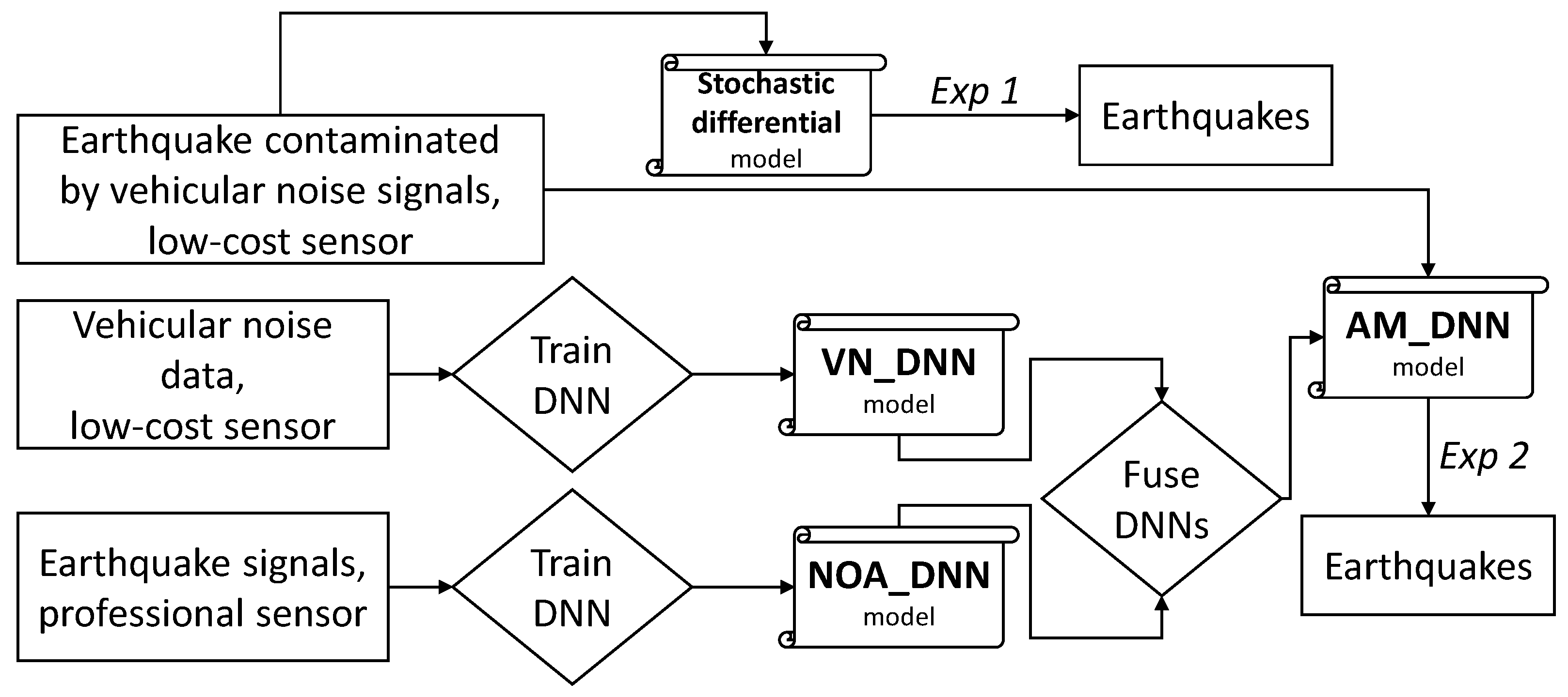
3. Proposed Methodology
3.1. A Stochastic Approach
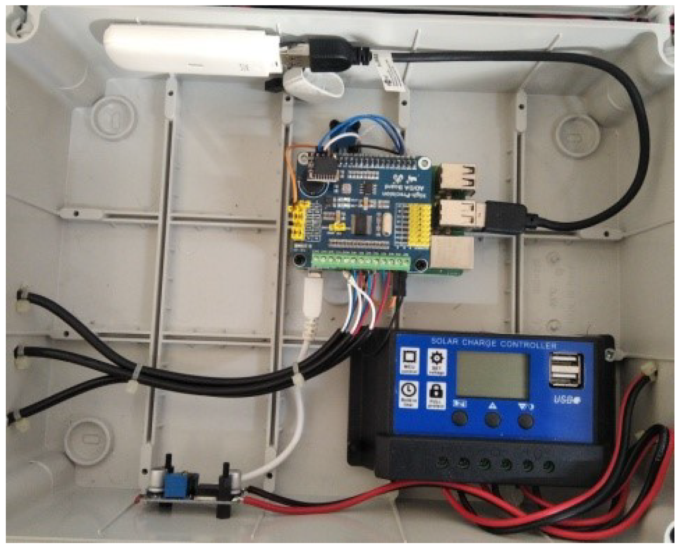
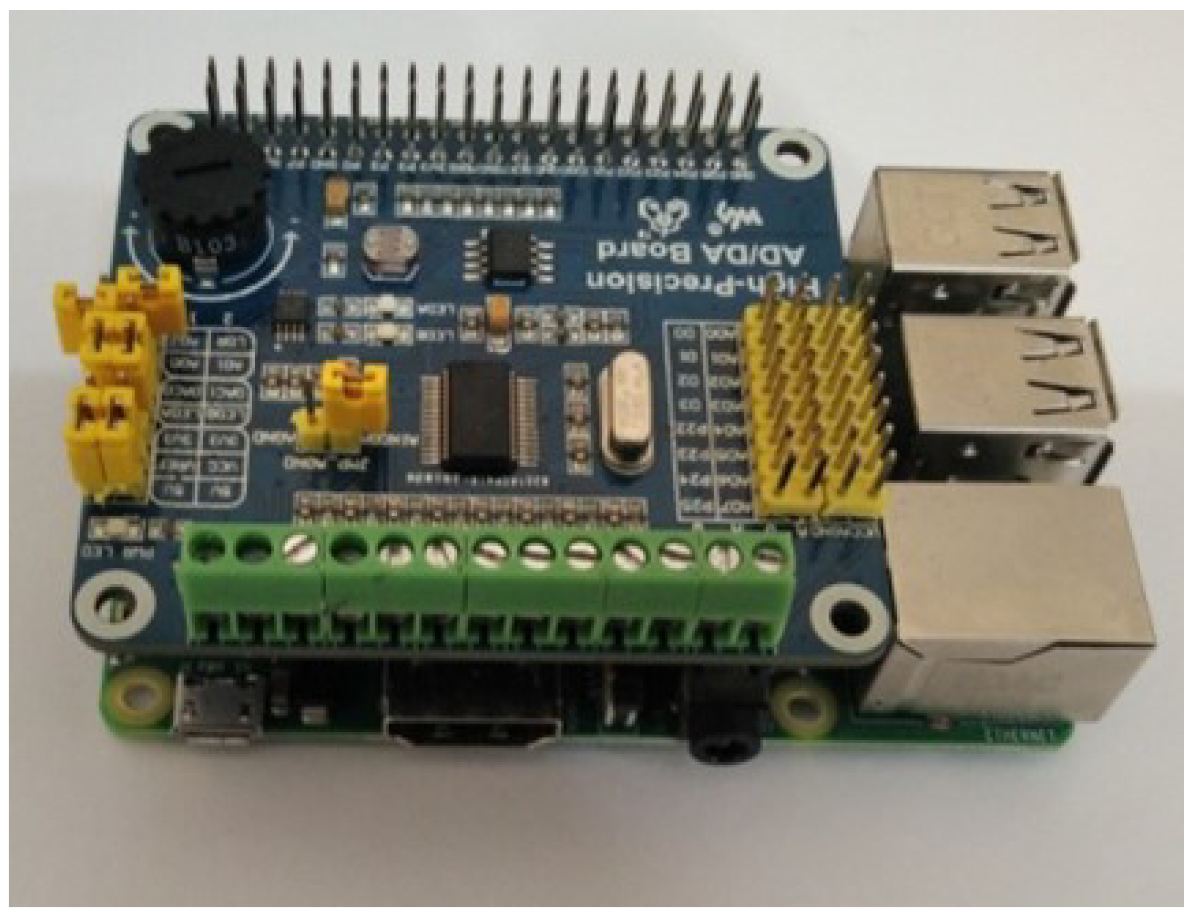
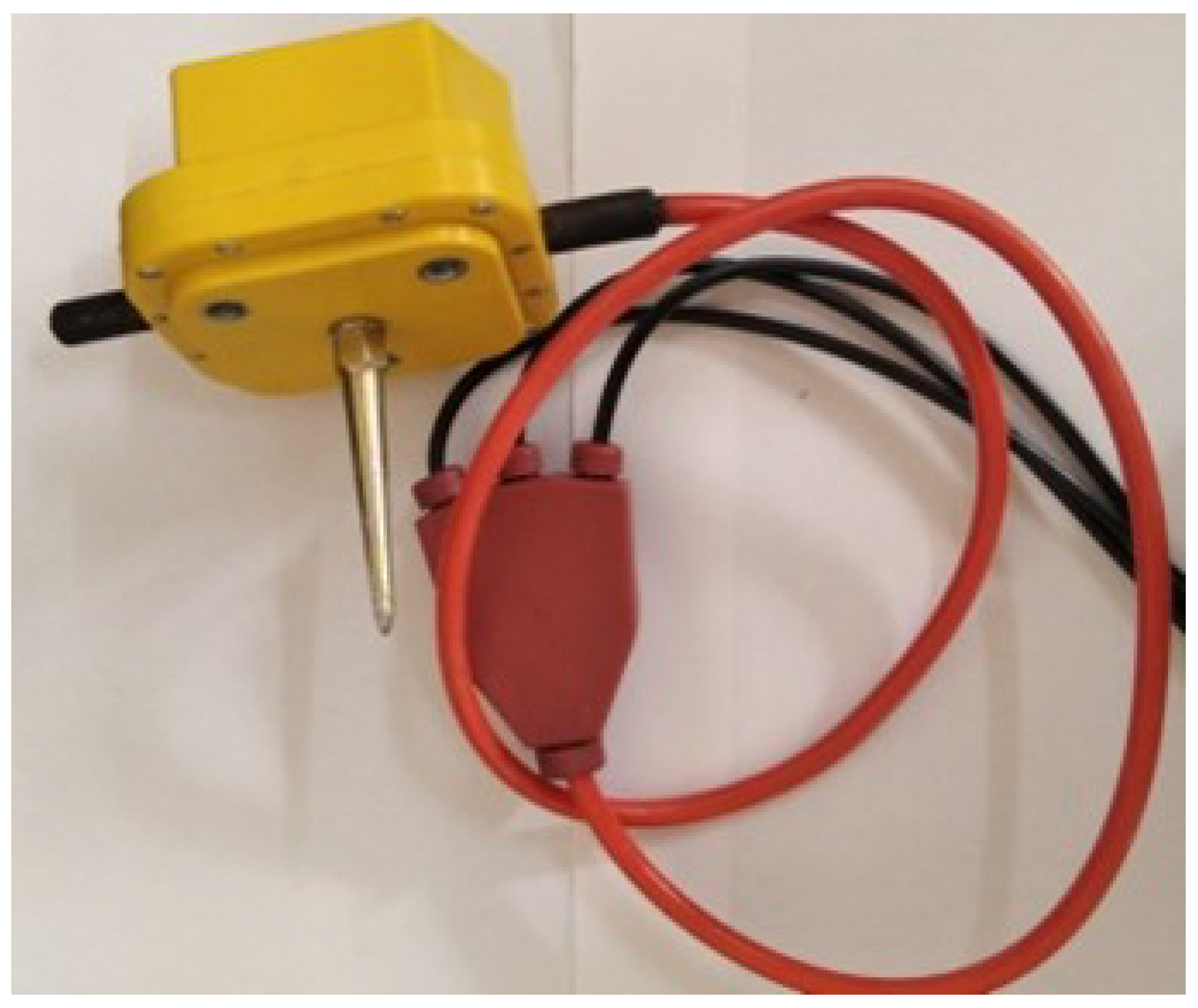
3.2. Low-Cost Seismic Sensory Equipment
3.3. Vehicular Noise
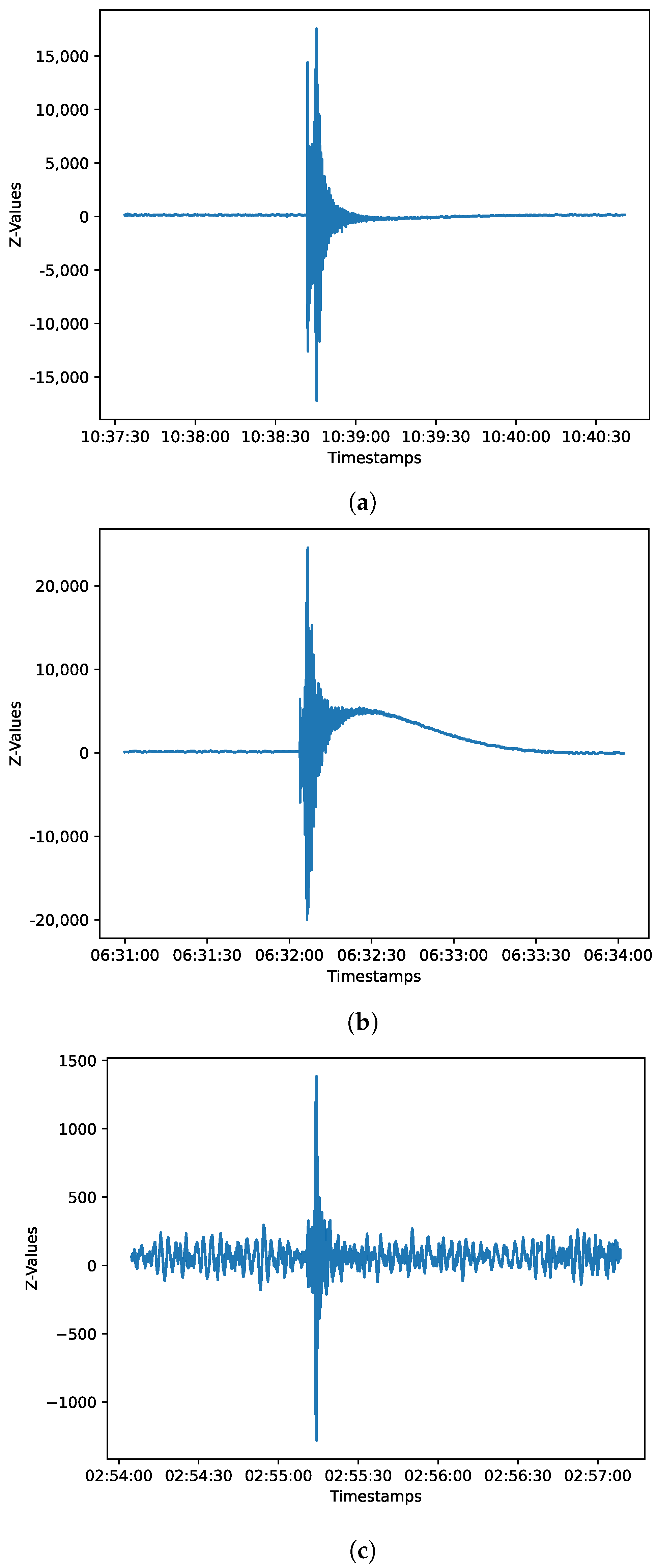
3.4. Ground Truth Earthquake Dataset
3.5. Training Process and Creation of DNNs
- Data preparation included several format conversion tasks aimed at converting the data into a proper form;
- Data normalization, wherein data were linearly normalized in the range of [−1, 1];
- Class imbalance handling, dealt with the imbalance of the dataset using the NearMiss method [31];
- Train–test split, where the available data were split in training and testing by means of a generic approach of an 80–20% split, so we could use enough data to train the models.
- A hidden LSTM (long short-term memory neural network) [35] layer with 64 units and a parameter, which returns the full sequence of outputs for each input sequence and allows stacking additional recurrent layers;
- A ‘flatten’ layer [2], which flattens the 3D output from the LSTM layer into a 2D tensor; this is typically done to connect the LSTM layer to a standard feed-forward neural network;
- An output layer, which is also a dense layer that represents the output of the model. The activation function used in this case is the sigmoid function [38], which outputs a probability score between 0 and 1.
3.6. Two-Fold Synchronized Dataset
4. Experimental Evaluation
4.1. Experimental Setup
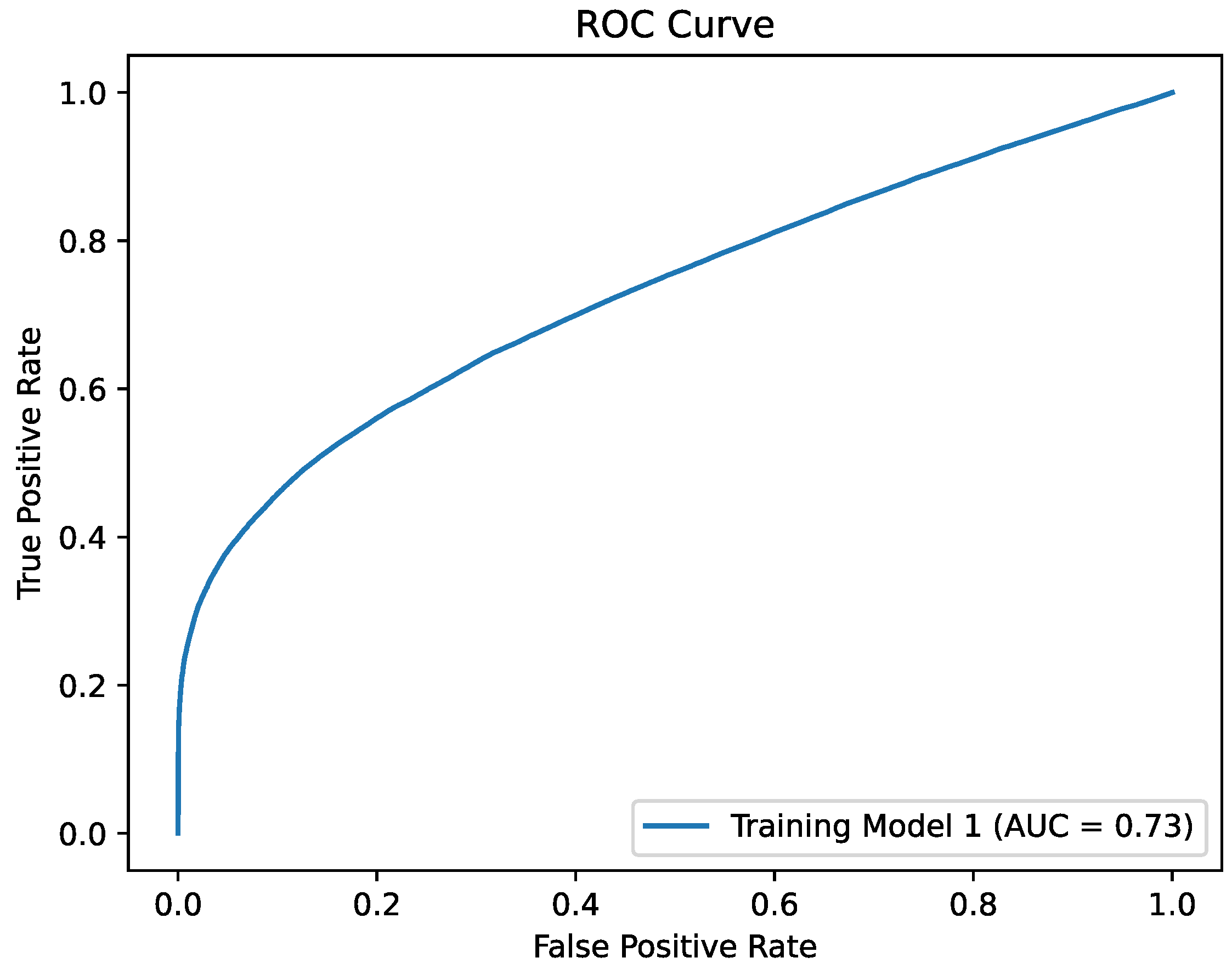
4.2. Training Model 1
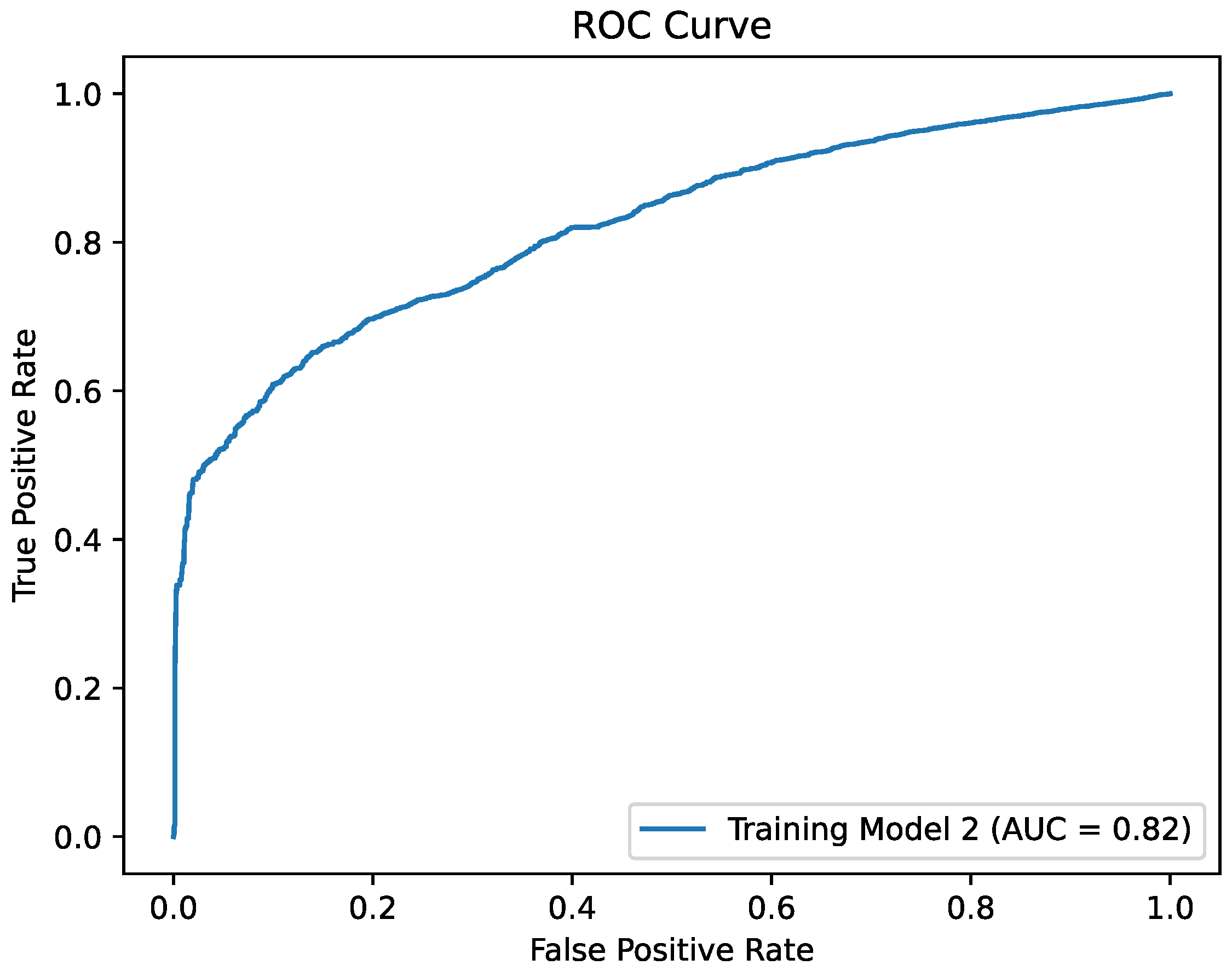
4.3. Training Model 2
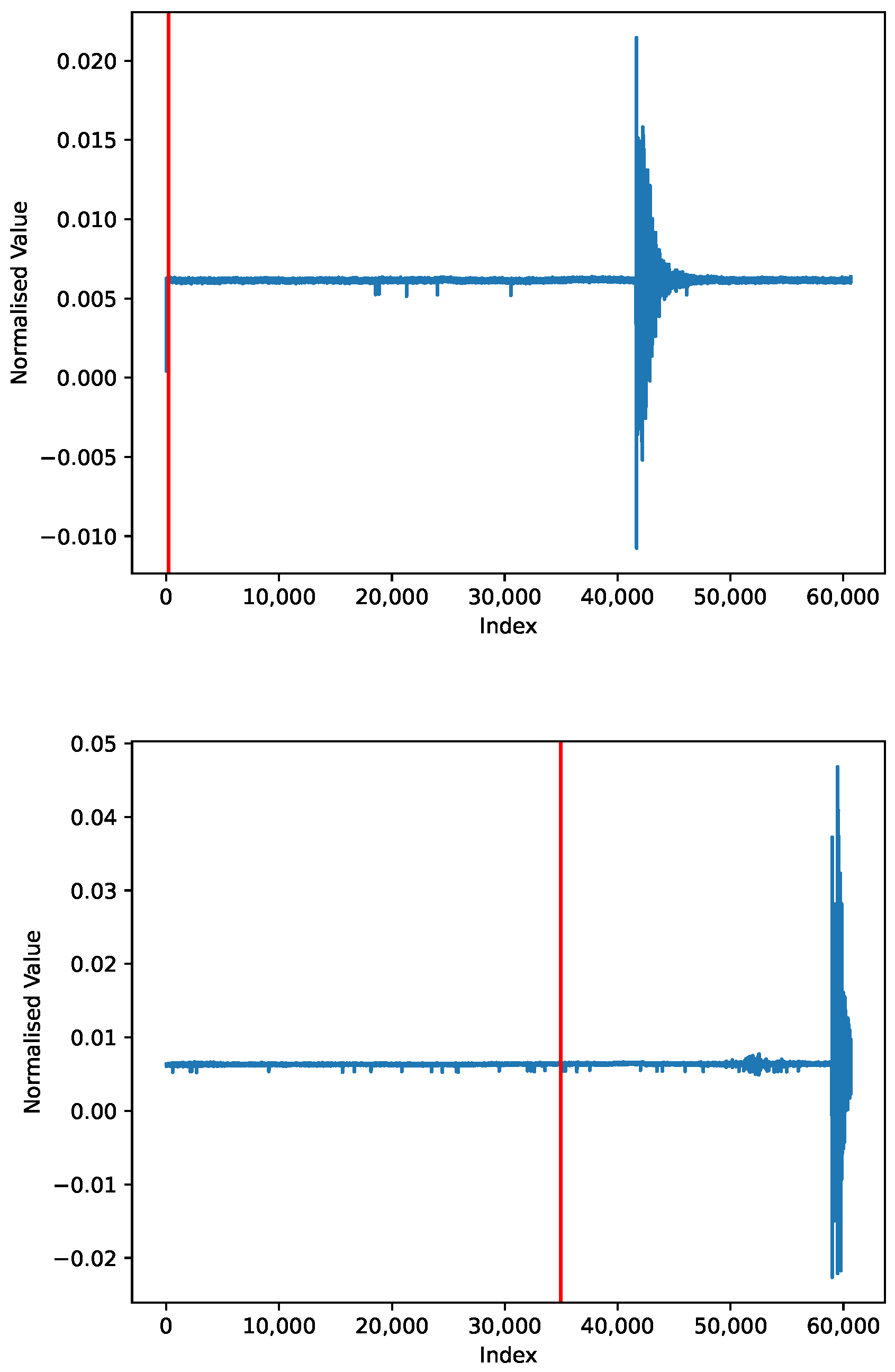
4.4. Experiment 1
4.5. Experiment 2
5. Conclusions
Author Contributions
Funding
Institutional Review Board Statement
Informed Consent Statement
Data Availability Statement
Conflicts of Interest
References
- Lim, J.; Jung, S.; JeGal, C.; Jung, G.; Yoo, J.H.; Gahm, J.K.; Song, G. LEQNet: Light Earthquake Deep Neural Network for Earthquake Detection and Phase Picking. Front. Earth Sci. 2022, 10, 848237. [Google Scholar] [CrossRef]
- Ji, L.; Zou, Y.; He, K.; Zhu, B. Carbon futures price forecasting based with ARIMA-CNN-LSTM model. Procedia Comput. Sci. 2019, 162, 33–38. [Google Scholar] [CrossRef]
- Murti, M.; Junior, R.; Najah, A.M.; Elshafie, A. Earthquake multi-classification detection based velocity and displacement data filtering using machine learning algorithms. Sci. Rep. 2022, 12, 21200. [Google Scholar] [CrossRef]
- Mousavi, S.M.; Sheng, Y.; Zhu, W.; Beroza, G.C. STanford EArthquake Dataset (STEAD): A Global Data Set of Seismic Signals for AI. IEEE Access 2019, 7, 179464–179476. [Google Scholar] [CrossRef]
- Mao, F.; Khamis, K.; Krause, S.; Clark, J.; Hannah, D.M. Low-cost environmental sensor networks: Recent advances and future directions. Front. Earth Sci. 2019, 7, 221. [Google Scholar] [CrossRef]
- D’Alessandro, A.; Scudero, S.; Vitale, G. A review of the capacitive MEMS for seismology. Sensors 2019, 19, 3093. [Google Scholar] [PubMed]
- Arora, N.; Kumar, Y. Automatic vehicle detection system in Day and Night Mode: Challenges, applications and panoramic review. Evol. Intell. 2023, 16, 1077–1095. [Google Scholar] [CrossRef]
- Mondal, B. Pandemic COVID-19, Reduced Usage of Public Transportation Systems and Urban Environmental Challenges: Few Evidences from India and West Bengal. In Environmental Management and Sustainability in India: Case Studies from West Bengal; Springer: Berlin/Heidelberg, Germany, 2023; pp. 341–368. [Google Scholar]
- Yu, Q.; Wang, C.; Li, J.; Xiong, R.; Pecht, M. Challenges and outlook for lithium-ion battery fault diagnosis methods from the laboratory to real world applications. eTransportation 2023, 17, 100254. [Google Scholar] [CrossRef]
- Bhatia, M.; Ahanger, T.A.; Manocha, A. Artificial intelligence based real-time earthquake prediction. Eng. Appl. Artif. Intell. 2023, 120, 105856. [Google Scholar] [CrossRef]
- Kassa, A.B.; Dugda, M.T.; Lin, Y.; Seifu, A. Earthquake Aftershocks Pattern Prediction. In Proceedings of the AGU Fall Meeting, Chicago, IL, USA, 12–16 December 2022; Volume 2022, p. S42C-0177. Available online: https://ui.adsabs.harvard.edu/abs/2022AGUFM.S42C0177D (accessed on 13 September 2023).
- Shearer, P.M. Introduction to Seismology: The Wave Equation and Body Waves; Institute of Geophysics and Planetary Physics; Scipps Institution of Oceanography; University of California: San Diego, CA, USA, 2010; unpublished. [Google Scholar]
- Udias, A.; Buforn, E. Principles of Seismology; Cambridge University Press: Cambridge, UK, 2017. [Google Scholar]
- Kennett, B.L.N. The Seismic Wavefield: Volume 1, Introduction and Theoretical Development; Cambridge University Press: Cambridge, UK, 2001; Volume 1. [Google Scholar]
- Hou, Y.; Jiao, R.; Yu, H. MEMS based geophones and seismometers. Sens. Actuators Phys. 2021, 318, 112498. [Google Scholar] [CrossRef]
- Bullen, K.E.; Bolt, B.A. An Introduction to the Theory of Seismology; Cambridge University Press: Cambridge, UK, 1985. [Google Scholar]
- Kumar, D.; Ahmed, I. Seismic Noise. In Encyclopedia of Solid Earth Geophysics; Gupta, H.K., Ed.; Springer International Publishing: Cham, Switzerland, 2021; pp. 1442–1447. [Google Scholar] [CrossRef]
- Dou, S.; Lindsey, N.; Wagner, A.M.; Daley, T.M.; Freifeld, B.; Robertson, M.; Peterson, J.; Ulrich, C.; Martin, E.R.; Ajo-Franklin, J.B. Distributed acoustic sensing for seismic monitoring of the near surface: A traffic-noise interferometry case study. Sci. Rep. 2017, 7, 11620. [Google Scholar] [CrossRef] [PubMed]
- Sun, L.; Qiu, X.; Wang, Y.; Wang, C. Seismic Periodic Noise Attenuation Based on Sparse Representation Using a Noise Dictionary. Appl. Sci. 2023, 13, 2835. [Google Scholar] [CrossRef]
- Du, R.; Liu, W.; Fu, X.; Meng, L.; Liu, Z. Random noise attenuation via convolutional neural network in seismic datasets. Alex. Eng. J. 2022, 61, 9901–9909. [Google Scholar] [CrossRef]
- Prasanna, R.; Chandrakumar, C.; Nandana, R.; Holden, C.; Punchihewa, A.; Becker, J.S.; Jeong, S.; Liyanage, N.; Ravishan, D.; Sampath, R.; et al. “Saving Precious Seconds”—A novel approach to implementing a low-cost earthquake early warning system with node-level detection and alert generation. Informatics 2022, 9, 25. [Google Scholar] [CrossRef]
- Wu, Y.M.; Mittal, H. A review on the development of earthquake warning system using low-cost sensors in Taiwan. Sensors 2021, 21, 7649. [Google Scholar] [CrossRef]
- Lee, J.; Khan, I.; Choi, S.; Kwon, Y.W. A smart iot device for detecting and responding to earthquakes. Electronics 2019, 8, 1546. [Google Scholar] [CrossRef]
- Ahmad, A.B.; Saibi, H.; Belkacem, A.N.; Tsuji, T. Vehicle Auto-Classification Using Machine Learning Algorithms Based on Seismic Fingerprinting. Computers 2022, 11, 148. [Google Scholar] [CrossRef]
- Nie, T.; Wang, S.; Wang, Y.; Tong, X.; Sun, F. An effective recognition of moving target seismic anomaly for security region based on deep bidirectional LSTM combined CNN. Multimed. Tools Appl. 2023. [Google Scholar] [CrossRef]
- Münchmeyer, J.; Woollam, J.; Rietbrock, A.; Tilmann, F.; Lange, D.; Bornstein, T.; Diehl, T.; Giunchi, C.; Haslinger, F.; Jozinović, D.; et al. Which Picker Fits My Data? A Quantitative Evaluation of Deep Learning Based Seismic Pickers. J. Geophys. Res. Solid Earth 2022, 127, e2021JB023499. [Google Scholar] [CrossRef]
- Avlonitis, M. On the problem of early detection of users interaction outbreaks via stochastic differential models. Eng. Appl. Artif. Intell. 2016, 51, 92–96. [Google Scholar] [CrossRef]
- Krischer, L.; Megies, T.; Barsch, R.; Beyreuther, M.; Lecocq, T.; Caudron, C.; Wassermann, J. ObsPy: A bridge for seismology into the scientific Python ecosystem. Comput. Sci. Discov. 2015, 8, 014003. [Google Scholar] [CrossRef]
- Evangelidis, C.P.; Triantafyllis, N.; Samios, M.; Boukouras, K.; Kontakos, K.; Ktenidou, O.; Fountoulakis, I.; Kalogeras, I.; Melis, N.S.; Galanis, O.; et al. Seismic Waveform Data from Greece and Cyprus: Integration, Archival, and Open Access. Seismol. Res. Lett. 2021, 92, 1672–1684. [Google Scholar] [CrossRef]
- Choubik, Y.; Mahmoudi, A.; Himmi, M.; El Moudnib, L. STA/LTA trigger algorithm implementation on a seismological dataset using Hadoop MapReduce. Iaes Int. J. Artif. Intell. (IJ-AI) 2020, 9, 269. [Google Scholar] [CrossRef]
- Mani, I.; Zhang, I. kNN approach to unbalanced data distributions: A case study involving information extraction. In Proceedings of the Workshop on Learning from Imbalanced Datasets, Washington, DC, USA, 21 August 2003; Volume 126, pp. 1–7. [Google Scholar]
- Abadi, M.; Barham, P.; Chen, J.; Chen, Z.; Davis, A.; Dean, J.; Devin, M.; Ghemawat, S.; Irving, G.; Isard, M.; et al. TensorFlow: A System for Large-Scale Machine Learning. In Proceedings of the 12th USENIX Conference on Operating Systems Design and Implementation, OSDI’16, Savannah, GA, USA, 2–4 November 2016; pp. 265–283. [Google Scholar]
- Chollet, F. Keras. 2015. Available online: https://keras.io (accessed on 13 September 2023).
- Hochreiter, S.; Schmidhuber, J. Long short-term memory. Neural Comput. 1997, 9, 1735–1780. [Google Scholar] [CrossRef]
- Kowsher, M.; Tahabilder, A.; Islam Sanjid, M.Z.; Prottasha, N.J.; Uddin, M.S.; Hossain, M.A.; Kader Jilani, M.A. LSTM-ANN & BiLSTM-ANN: Hybrid deep learning models for enhanced classification accuracy. Procedia Comput. Sci. 2021, 193, 131–140. [Google Scholar] [CrossRef]
- Abualhaol, I.; Falcon, R.; Abielmona, R.; Petriu, E. Data-Driven Vessel Service Time Forecasting using Long Short-Term Memory Recurrent Neural Networks. In Proceedings of the 2018 IEEE International Conference on Big Data (Big Data), Seattle, WA, USA, 10–13 December 2018; Volume 12, pp. 2580–2590. [Google Scholar] [CrossRef]
- Agarap, A.F. Deep Learning using Rectified Linear Units (ReLU). arXiv 2018, arXiv:1803.08375. [Google Scholar]
- Dubey, S.R.; Singh, S.K.; Chaudhuri, B.B. A Comprehensive Survey and Performance Analysis of Activation Functions in Deep Learning. arXiv 2021, arXiv:2109.14545. [Google Scholar]
- Yang, T.; Ying, Y. AUC Maximization in the Era of Big Data and AI: A Survey. arXiv 2022, arXiv:2203.15046. [Google Scholar] [CrossRef]

| Accuracy | Precision | Recall | F1 Score | AUC Curve |
|---|---|---|---|---|
| 68% | 77% | 52% | 69% | 73% |
| Accuracy | Precision | Recall | F1 Score | AUC Curve |
|---|---|---|---|---|
| 75% | 83% | 63% | 72% | 82% |
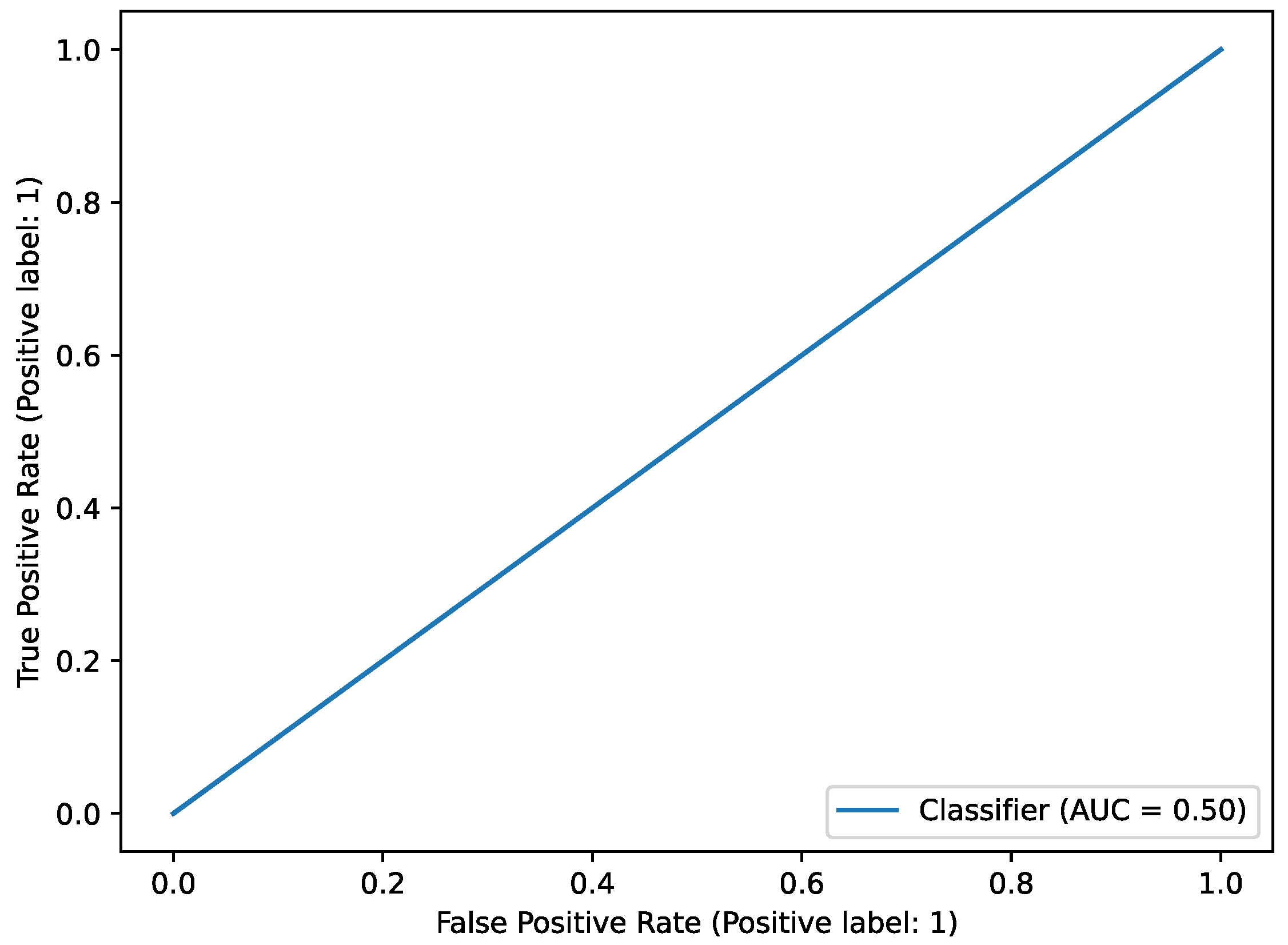
| Accuracy | Precision | Recall | F1 Score | AUC Curve |
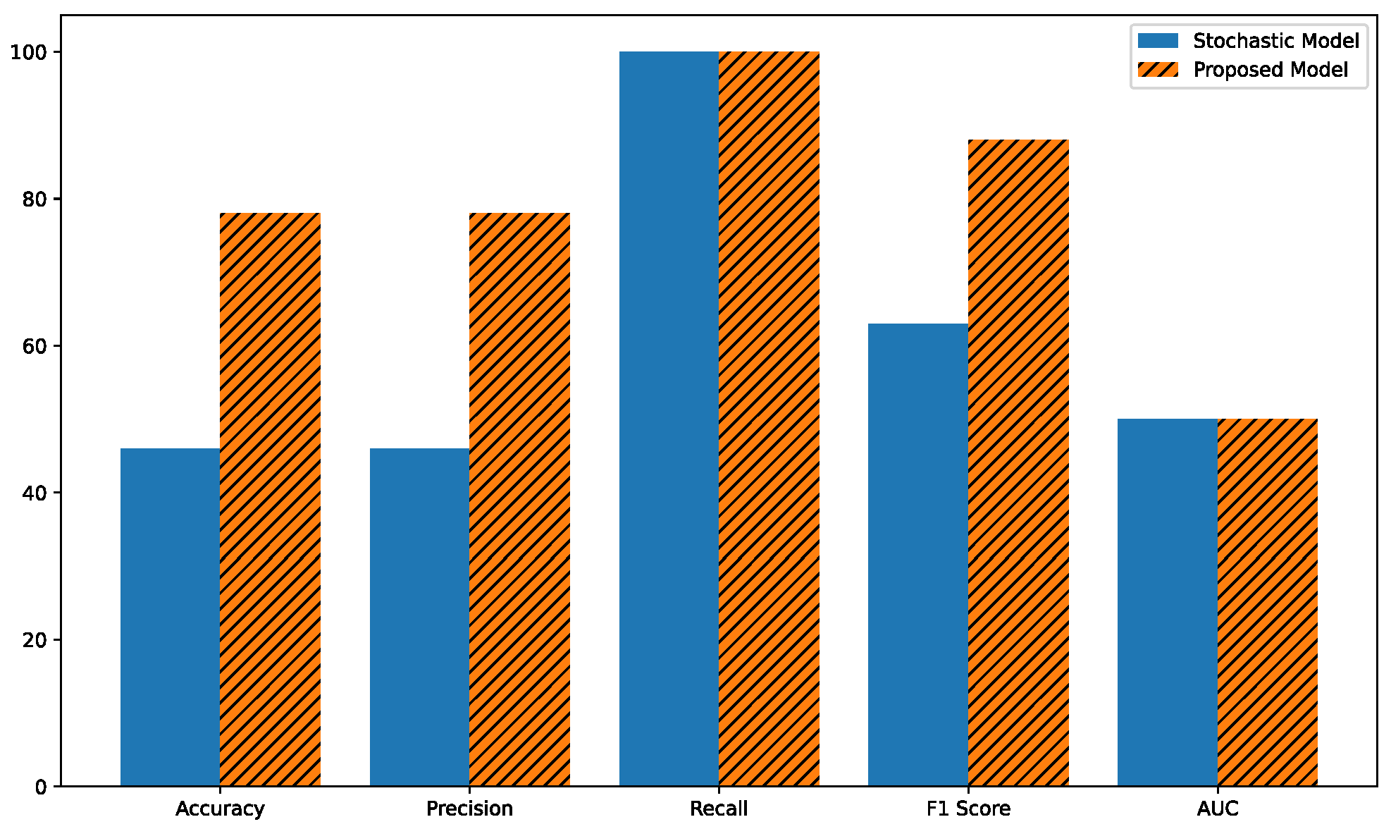
|---|---|---|---|---|
| 46% | 46% | 100% | 63% | 50% |
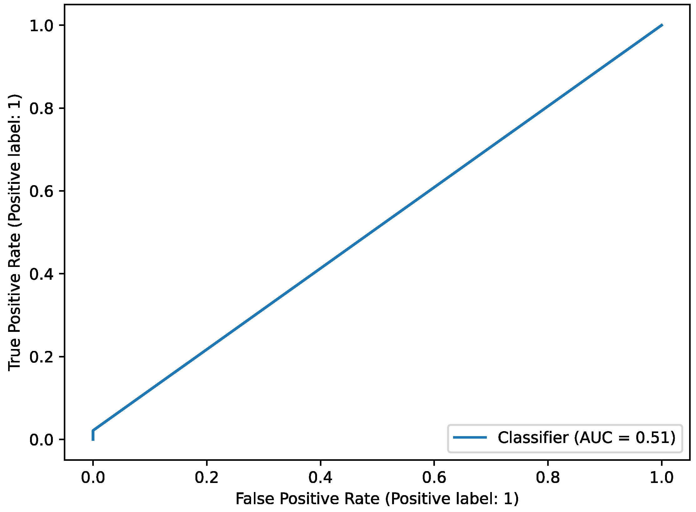
| Accuracy | Precision | Recall | F1 Score | AUC Curve |
|---|---|---|---|---|
| 78% | 78% | 100% | 88% | 51% |
Disclaimer/Publisher’s Note: The statements, opinions and data contained in all publications are solely those of the individual author(s) and contributor(s) and not of MDPI and/or the editor(s). MDPI and/or the editor(s) disclaim responsibility for any injury to people or property resulting from any ideas, methods, instructions or products referred to in the content. |
© 2023 by the authors. Licensee MDPI, Basel, Switzerland. This article is an open access article distributed under the terms and conditions of the Creative Commons Attribution (CC BY) license (https://creativecommons.org/licenses/by/4.0/).
Share and Cite
Agathos, L.; Avgoustis, A.; Avgoustis, N.; Vlachos, I.; Karydis, I.; Avlonitis, M. Identifying Earthquakes in Low-Cost Sensor Signals Contaminated with Vehicular Noise. Appl. Sci. 2023, 13, 10884. https://doi.org/10.3390/app131910884
Agathos L, Avgoustis A, Avgoustis N, Vlachos I, Karydis I, Avlonitis M. Identifying Earthquakes in Low-Cost Sensor Signals Contaminated with Vehicular Noise. Applied Sciences. 2023; 13(19):10884. https://doi.org/10.3390/app131910884
Chicago/Turabian StyleAgathos, Leonidas, Andreas Avgoustis, Nikolaos Avgoustis, Ioannis Vlachos, Ioannis Karydis, and Markos Avlonitis. 2023. "Identifying Earthquakes in Low-Cost Sensor Signals Contaminated with Vehicular Noise" Applied Sciences 13, no. 19: 10884. https://doi.org/10.3390/app131910884
APA StyleAgathos, L., Avgoustis, A., Avgoustis, N., Vlachos, I., Karydis, I., & Avlonitis, M. (2023). Identifying Earthquakes in Low-Cost Sensor Signals Contaminated with Vehicular Noise. Applied Sciences, 13(19), 10884. https://doi.org/10.3390/app131910884