Abstract
With the development of the Internet of Things (IoT), most communication systems are difficult to implement on a large scale due to their high complexity. Multiple-input multiple-output (MIMO) precoding is a generally used technique for improving the reliability of free-space optical (FSO) communications, which is a key technology in the 6G era. However, traditional MIMO precoding schemes are typically designed based on the assumption of additive white Gaussian noise (AWGN). In this paper, we present a novel MIMO precoding method based on reinforcement learning (RL) that is specifically designed for the Poisson shot noise model. Unlike traditional MIMO precoding schemes, our proposed scheme takes into account the unique statistical characteristics of Poisson shot noise. Our approach achieves significant performance gains compared to existing MIMO precoding schemes. The proposed scheme can achieve the bit error rate (BER) of in a strong turbulence channel and exhibits superior robustness against imperfect channel state information (CSI).
1. Introduction
With the massive growth of data transmission, the future Internet of Things (IoT) will face more severe challenges. Free-space optical (FSO) communication is crucial in the forthcoming 6G era, with its characteristics of wide bandwidth, high speed, and high capacity [1]. Multiple-input multiple-output (MIMO) technology has been proven by multiple studies to be equally applicable to FSO systems. In FSO communication, MIMO is applied to reduce turbulence-induced fading. Instead of using a single transmitter and receiver, FSO MIMO systems employ multiple transmitters and receivers along with an array of optical elements such as laser diodes and detectors. These elements are strategically positioned to create multiple optical channels for data transmission. The application of MIMO to FSO systems offers significant advantages in terms of data rate, reliability, and robustness [2,3].
Ultraviolet (UV) communication has the characteristics of support for non-line-of-sight (NLOS) communication [4], and good confidentiality performance, which has attracted extensive attention. UV communication can be utilized in various scenarios. On-the-move communication is made possible through UV-C links, enabling devices in vehicles or drones to communicate seamlessly. Additionally, UV communication proves beneficial in IoT applications, facilitating communication between devices in harsh environments. Moreover, UV communication enables machine-to-machine communication, allowing machines or sensors to exchange data even in environments with high interference or restricted line-of-sight [5].
The atmospheric turbulence effect caused by random fluctuations in the atmosphere can seriously affect the communication quality of FSO systems. To solve these problems, precoding techniques are used at the transmitter to combat turbulence [6,7,8]. However, it should be pointed out that traditional precoding methods are derived from the additive white Gaussian noise (AWGN) model. Optical communication systems use light to transmit data, and light consists of discrete particles known as photons. The arrival of photons at the receiver’s detector follows a Poisson process, where photons are emitted randomly over time. The Poisson shot noise model accurately captures this discrete nature of optical signals, making it a better fit for optical communication systems. In other words, the optical communication models are generally modeled as signal-related Poisson shot noise [9,10]. Precoders and detectors designed under the AWGN model are no longer suitable for photon-counting communication systems. The precoder and combiner should be redesigned for the Poisson shot noise model.
The studies regarding the combination of communication and artificial intelligence (AI) have attracted widespread attention from scholars [11,12,13], which is a novel way to solve problems in mobile communication. The authors of [11] jointly design the active beamforming and passive beamforming to maximize the sum rate, using the deep deterministic policy gradient (DDPG) algorithm. The action space of this algorithm is designed by the beamforming matrix and the phase shift matrix. In [12], the authors utilize soft actor–critic (SAC) algorithm to design active analog precoder and passive beamformer. The authors of [13] propose a DRL-based precoding framework in both codebook-based and non-codebook-based MIMO precoding systems and examine the performance of the DQN and DDPG algorithms. The advantage of combining reinforcement learning (RL) and mobile communication is that different features can be extracted from a large number of raw data, and by learning to continuously adjust the parameter settings in the internal structure, RL can flexibly approximate the mathematical model of the simulated communication environment and deal with some complex physical channels. RL is applied in practice in various domains such as robotics, navigation, and smart grids. In robotics, RL can be used to train robotic arms to perform tasks like opening doors and picking up objects. RL is also used in navigation systems to optimize routes and make decisions based on real-time data. However, there are some potential challenges in applying RL. One challenge is the long time it takes for RL algorithms to converge and learn something meaningful. This restricts the use of RL techniques in real-time learning scenarios. Another challenge is the need for large numbers of data for training RL models. RL algorithms require extensive exploration of the environment to learn optimal policies, which can be time-consuming and resource-intensive. Additionally, RL algorithms may struggle with partial observability and uncertainty in complex environments, which can affect their performance and ability to make accurate decisions [14,15].
The non-convex problem and coupling constraints, as studied in this paper, pose considerable challenges to finding an optimal solution. In order to address this, we propose a novel MIMO precoding scheme based on RL, which provides a highly effective approach for jointly optimizing both the precoding and detection matrix of the transceiver and receiver, respectively. The proposed RL-based solution offers a number of key advantages over traditional optimization methods, such as greater flexibility and the adoption of the variation of system dynamics. Specifically, the RL framework allows the system to learn from past experiences and optimize the transmission and reception processes in an iterative and adaptive manner. Overall, our findings highlight the potential of RL-based methods for addressing complex optimization problems in FSO communication systems.
In this study, a joint precoder and combiner optimization based on RL is proposed. We analyze the bit error rate (BER) performance at different system parameters and compare it with the conventional schemes. The simulation results show that our scheme is able to obtain a lower BER performance compared to the conventional scheme. The main contributions of this research include:
- 1.
- Our proposal involves the introduction of a state-of-the-art NLOS UV MIMO system, which is capable of photon-counting while operating under the influence of Poisson shot noise. To optimize the system performance, we formulate a novel optimization problem that addresses the design of both the precoding and combining matrices, utilizing the well-established minimum mean square error (MMSE) criterion.
- 2.
- By employing a methodical approach to deriving and reformulating key aspects of our expected MMSE precoding design, we successfully transform it into an optimization problem that is conducive to efficient computation using the multi-agent deep deterministic policy gradient (MADDPG) algorithm [16]. Through this novel approach, we are able to attain the global optimal precoding matrix and combining matrix.
- 3.
- The proposed system exhibits strong robustness. To evaluate the efficacy of our approach in realistic settings, we conducted experiments considering varying degrees of channel state information (CSI). The simulation results indicate our scheme is capable of achieving a BER of less than even when the CSI is imperfect.
The rest of this paper is organized as follows. The related work is presented in Section 2. Section 3 introduces the system model. In Section 4, we present the RL-based precoder and combiner design, in which a specific expression of the optimization problem is given by a detailed mathematical derivation. In Section 5, we propose a method to solve the optimization problem based on the MADDPG algorithm. The simulation results are given in Section 6. Finally, we conclude in Section 7.
2. Related Work
Recently, various studies have been published in the area of photon-counting systems. In [17], the design of a MIMO system under the Poisson model is considered, in which a pulse-position modulation (PPM) modulation is used at the transmitter side, a maximum likelihood (ML) detection algorithm under the Poisson model is derived, and optimal as well as sub-optimal decoders are given. In [18], a receiver based on the linear least mean square error (MSE) criterion for FSO communication is presented. The system BER performance is analyzed under on–off keying (OOK) and PPM modulation. In [19], the statistical behavior of underwater fading with different probability density functions (PDFs) is studied. In [20], the authors present a composite quantum iterative multistage measurer and MIMO detector at the receiver. In [21], the analytical error probabilities for ML detection in turbulent and non-turbulent cases are derived. In [22], to minimize the probability of detection errors given relay forwarding power budget, a counting and forward relay framework for NLOS communication is presented. In [23], the communication capacity and performance of the Poisson model are investigated. And an upper limit of capacity and a lower limit of error probability are proposed. In [24], the photonic information rate is investigated for a single-photon avalanche diode (SPAD) array, and the effect of dead time on the system is considered. The results show that the photon-counting distribution can be regarded as a Gaussian distribution for sufficiently large arrays.
The conventional millimeter-wave hybrid precoding design method mainly decouples the hybrid precoding problem into transmitter-side hybrid precoding design and receiver-side hybrid combiner design, and it regards these two subproblems as matrix decomposition problems, respectively. The hybrid precoding problem is solved by minimizing the Euclidean distance between the product of the analog and digital matrices and the optimal all-digital precoding matrix under unconstrained conditions. In [25], a hybrid precoding method based on the alternating directional multiplier method (ADMM) is proposed. In [26], the symbol-level precoding of a MU-MISO downlink system is investigated. In [27], the objective function of the considered precoding scheme is highly nonconvex and has some complicated constraints, and the authors design a new method based on the ADMM. The convergence conditions of the proposed method are given by considering the order of iterations of the variables. In [28], the design of the symbol-level precoder for MU-MISO downlink communication is investigated, and its decision boundary is studied through the minimum maximum fairness design. To deal with this problem, the dimensionality of the variables is firstly reduced by solving a relaxation problem, after which the ADMM framework is used to efficiently solve the problem.
UV has the characteristics of high interference immunity, good confidentiality, and support for non-visual transmission, thus attracting the attention of a large number of researchers. In [29], the authors calculate the optical loss in the FSO communication system operating in the non-visual range, where scattering effects were taken into account, and the obtained results were compared with experimental data at 265 nm (solar-blind UV region). In [30], a 1 × 4 communication system was built. The experimental results show that equal-gain combining can provide significant diversity gain, provided that the transmit elevation angle is small or the transceiver distance is short. In [31], wireless UV communication is applied to UAV communication systems to solve the problem of directional awareness. In [32], the spatial diversity technique for the NLOS UV system is investigated, and the BER for different transmitter and receiver configurations is derived.
Recently, the concept of intelligent communication has attracted a considerable amount of attention, and its use of machine learning-based methods to deal with optimization problems in communication systems has achieved superior performance. In [33], an optimal hybrid precoding scheme based on hybrid cross entropy (HCE) is designed to maximize the total achievable rate. In [34], the authors design the selection and precoding matrices jointly for millimeter-wave systems. The proposed framework contains a neural network (NN) based on deep reinforcement learning (DRL) and a deep deployment NN. In [35], a user grouping algorithm based on channel gain and correlation is designed, and then a beam space orthogonal simulation precoder is obtained using DRL-based beam selection.
3. System Model
This section introduces the theoretical basis of the photon-counting MIMO system; the system model of each technology will be further explained below.
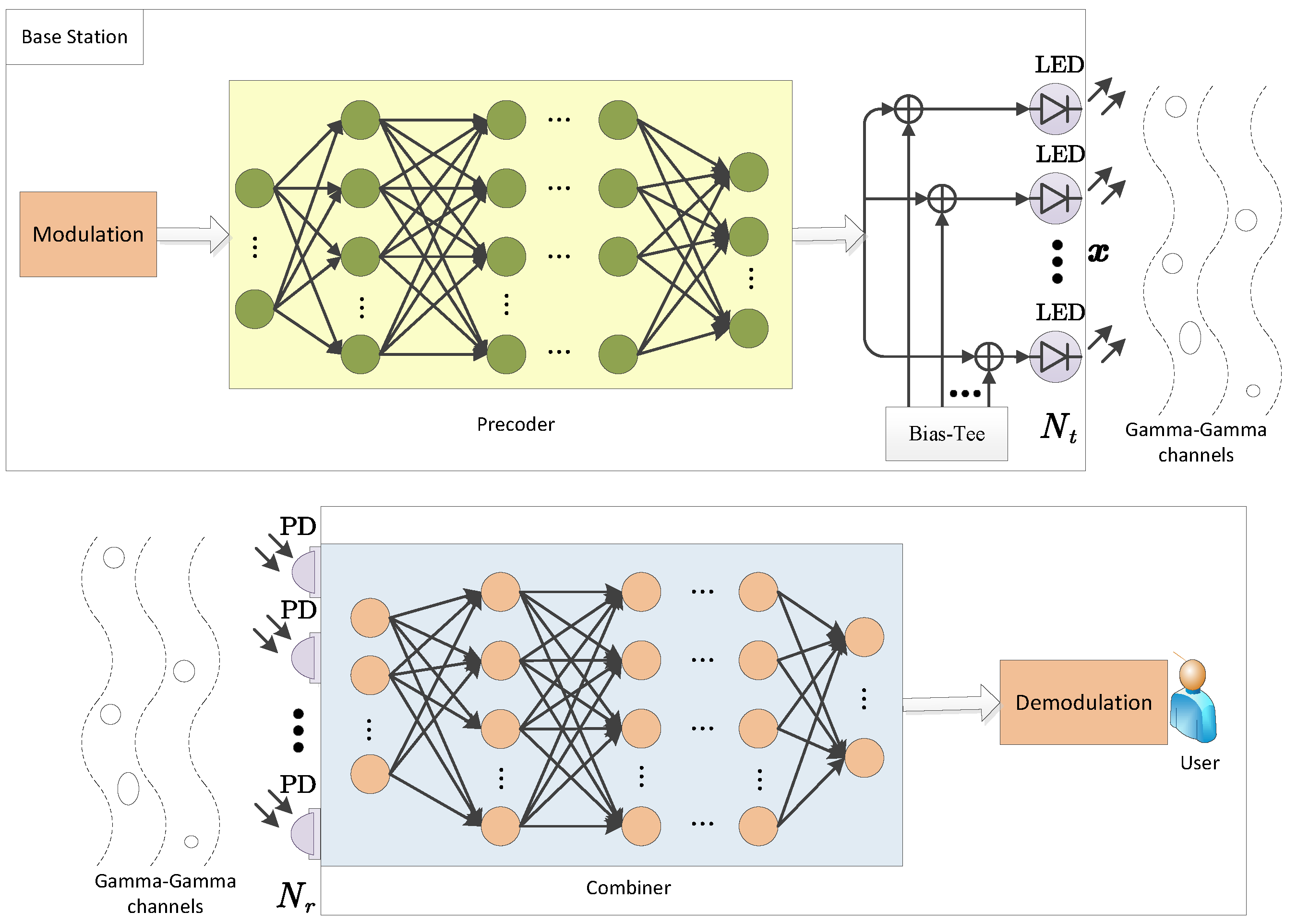
As presented in Figure 1, the considered photon-counting MIMO downlink system has light-emitting diodes (LEDs) in the base station (BS) that transmit data streams collaboratively to the photo detector (PD). Assume that the number of data streams and PDs is identical () and that the data streams are uncorrelated. The precoded signal is , where represents the data streams, and is the precoding matrix. To ensure the non-negativity of the signals, a direct current (DC) bias is appended to the transmit symbols through bias-ttee circuits. Therefore, the input signal of the LED is , driving the LEDs to transmit the signal through the FSO turbulent fading channels.
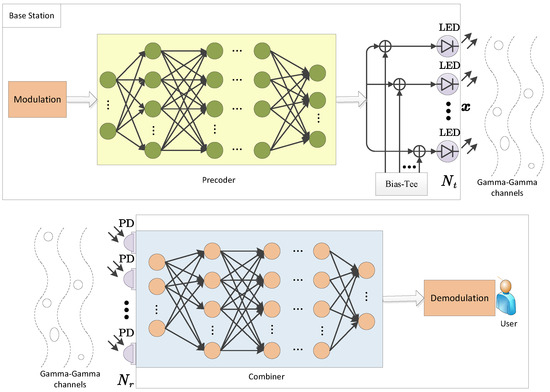
Figure 1.
System block diagram of the UV NLOS MIMO.
Free-space light transmits data to the PD through an optical medium via LEDs. FSO systems encounter several challenges during transmition, such as shadows when the lighting location is blocked from an area, which leads to information loss. The channel irradiance between the i-th PD and the j-th LED is denoted by , which obeys the gamma–gamma distribution with the PDF:
where is the standard gamma function, and are the distribution shaping parameters satisfying:
where , , is the light wave factor; represents the wavelength; D is the diameter of the aperture of the condenser at the receiver; L is the distance of the link; and represents the index value of the refractive structure parameter and is a function of altitude h.
The i-th PD’s channel matrix is ; hence, the channel matrix between the user and the BS is denoted by
The photon-counting process model is adopted at the receiver. The random variable corresponding to the number of photons detected by the j-th PD, denoted by , follows the Poisson distribution with the PDF:
In (5), is the number of noise photons generated by background radiation, where is the PD efficiency, is the background radiation power, T is the duration of a symbol, h is Planck’s constant, and f is the center frequency.
After removing the DC bias, the received signal follows:
The received signal from the transmitter is typically subject to various forms of interference and distortion during propagating through the channel. This results in a degraded signal at the receiver, which requires further promotion in order to extract useful information. Hence, a combiner matrix is typically used to combine the received signals from PD at the receiver. The combiner matrix is used to combine the received signal across PDs.
Assuming independent numbers of received photons across all PDs, the combined signal can be used to estimate the coded bit. This involves decoding the received signal and extracting the transmitted information from it.
4. Problem Formulate
In this section, we design the precoder and combiner according to the MMSE principle with detailed mathematical derivation and propose the form of the optimization problem. By solving this optimization problem, we are able to derive the optimal precoder and combiner that minimize the MSE of the received and transmitted signals.
We take the MSE as the performance measure and optimization objective for the joint precoder and combiner design, which is defined as
where the expectation is taken over variables and . Consider OOK modulation in the BS, and equal probability for the code bit , i.e., [36]. Hence,
Define the correlation matrix . Then, we have
First, we have that is given by
For , we have
Define a set with alphabet size , where each element of has the a priori probability . Then, (11) can further expand as
Based on (6), we have . Since for a randome varaible X, (12) is equal to
Note that we have used the fact that and based on our definition.
For , we have
According to (13) and (14), we have that
Next, is given by
For , we have
Note that we use the conclusion that and , and the proof is given in Appendix A. According to (17), we have that
According to (8), (15), and (18), the closed form of the MSE is
In order to make the LED work within a linear dynamic range, the transmit signal satisfies
where and represent the minimum and maximum currents corresponding to the linear dynamic range, respectively. Since
adding DC bias to (21) yields
To satisfy the constraint in (20), we have
(23) can be further expressed as
where D is given by
The optimization problem can thus be formulated as
where is the maximum linear optical power of the LEDs. For optical communications, the transmit signals must be non-negative. The emitting power of the LED also needs to be within its dynamic range [, ]. These factors lead to the constrains.
5. Precoder and Combiner Design Based on Reinforcement Learning
The optimization problem mentioned in Equation (26) is obviously a NP-hard problem, which cannot be solved via conventional optimization solvers. Hence, we proposed an RL-based approach to jointly solve the precoding matrix and the combining matrix. Several researchers of beamforming employed the deep Q network (DQN) to find optimal solutions. DQN is designed to solve tasks with discrete action space. To utilize DQN in continuous action space, we need to discretize the continuous action space, which will make the action space grow exponentially with the size of network [37]. While the DDPG algorithm can be used in continuous action space, the MADDPG can in addition reduce the action dimension of single agent. In the case of the joint design of the precoding matrix and combining matrix, MADDPG may be appropriate as it allows for decentralized decision-making while considering global state information. MADDPG enables each agent to interact with the environment and learn its own strategy based on local observations and rewards while also considering the joint actions and rewards of other data streams. The choice of MADDPG for jointly designing precoding and combining matrices may be based on its ability to handle multi-agent scenarios, its abikity to handle continuous action spaces, and its use of target networks and experience replay for stability and efficiency. To employ an RL method, we model the process of generating the precoding and combining matrix into the Markov decision process (MDP). Then, we apply the MADDPG algorithm to explore the optimal policy of the MDP. The elements of MDP and the MADDPG algorithm will be presented in the following, respectively. In the context of optimizing precoding and combining matrices, MADDPG can be used to train a network of agents, where each agent represents a communication node equipped with multiple antennas. The agents collaborate to learn the optimal strategies for precoding and combining matrices, taking into account the interactions and dependencies among the nodes.
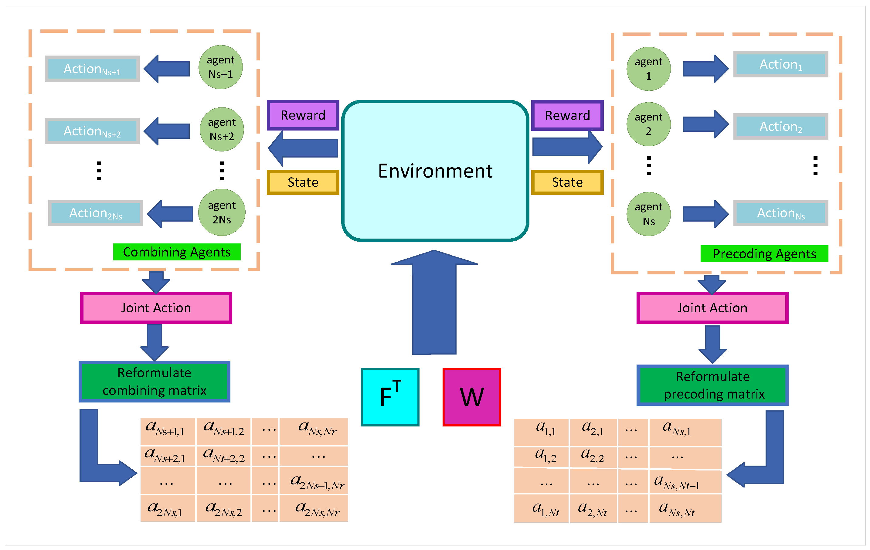
Figure 2 is the framework of the MADDPG-based joint precoding and combing algorithm, which consists of two sets of the same number of agents and an interactive environment. The agents receive the states and rewards transmitted by the environment and output corresponding actions, which are recombined into a precoding/combing matrix, respectively, allowing the environment to compute and output new states and rewards.
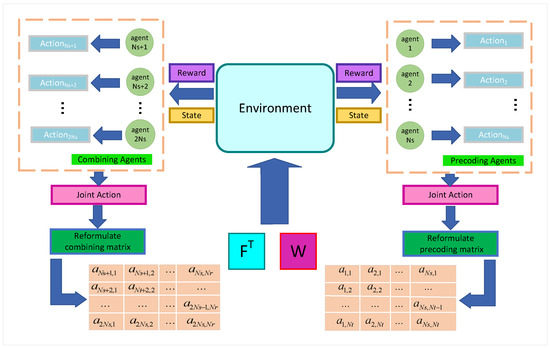
Figure 2.
The framework of MADDPG-based joint precoding and combining algorithm.
5.1. Agent
Since the dimensions of the precoding and combining matrices to be optimized do not coincide, two sets of agents with different action dimensions are set to form the part of solving the precoding and combining matrices. For the state of each agent, characterized as the L2-norm value of each row of the interactively generated precoding matrix and combine matrix, the set of state dimensions and the set of action dimensions of the agent are denoted as and .
5.2. State Space
In the t-th iteration, given the environment state of the current agent i, the joint state space of multiple agents at iteration step t is represented as . One precoding and combining agent only obtains its own state information, which is the L2-norm value of the row vector corresponding to the or matrix according to the agent allocation situation, while the states as well as actions information of other agents are unknown. That is, the state observed by the agent i is or .
5.3. Action Space
The action output of one agent constitutes the elements of one row of the matrix. The action outputs of all agents compose the whole matrix. The elements of the matrix are continuous real numbers, and in the agent action design, the action output range is [−1,1], that is, the matrix elements are normalized to the range [−1,1], and the action dimension of the agent is designed according to . In the t-th iteration, the actor network of the i-th agent outputs the action according to the current policy. The joint action is denoted as . The agents interact with the environment through the joint action and obtain the reward and the -th state information . For the reward, all of the agents obtain the same reward from the interaction with the system environment to prompt cooperative behaviors among the agents.
5.4. Reward Function
The focus of whether RL can better solve the optimization problem lies in the reward function. In the precoding optimization problem of the downlink MIMO system, the joint optimization problem of the precoding matrix and combining matrix can be reduced to a minimization MSE problem. The optimization problem is shown in (26).
Due to the existence of constraints, the reward function designed in this paper is divided into two parts: one is the desired optimization objective, and another one is the penalty term for not satisfying the constraints. The first part of the reward function is
The second part of the reward function is the penalty term, which is set to for any constraint that is not satisfied. Since the MSE value should be positive, consider increasing the penalty when . This penalty term is set to , which means that
The second part of the reward function can be expressed as
In summary, the ultimate reward of MDP can be represented as the linear combination of optimization objective and the penalty term.
5.5. Joint Precoding and Combining Algorithm Based on MADDPG
MADDPG is actor–critic algorithm that utilizes the idea of centralized training and decentralized decision-making. The actor makes a decision over time steps, while the critic evaluates the value of the decision. Assume the set is the policies of all agents and set as the parameters of corresponding policies. For the i-th agent’s policy , the object function is the expected reward. The gradient of the object function w.r.t can be depicted as:
where , . is the replay buffer, which stores the transition , where is the next time step state and . is the Q-value function. The Q-function can be updated by minimizing the function below:
In (34), , is the Q-value discounting factor, and represents the policies with the delayed network parameter . Each agent maintains two sets of actor–critic network pairs, known as the behavior pair and the target pair. Relative to the behavior pair, the target pair of networks makes a soft replacement with parameters. We show the algorithm as a pseudo-code type in Algorithm 1.
The hyperparameters of MADDPG are shown in Table 1.
| Algorithm 1: MADDPG for joint precoding and combining optimization | |||||||
| 1 | Start; | ||||||
| 2 | Initialize the environment of downlink MIMO communication system; | ||||||
| 3 | Randomly initialize the weights of behavior actor–critic pair; | ||||||
| 4 | for episode = do | ||||||
| 5 | Initialize a Gaussian random process ; | ||||||
| 6 | Reset the photon-counting MIMO downlink system environment and obtain initial global state ; | ||||||
| 7 | for do | ||||||
| 8 | Each agent selects action ; | ||||||
| 9 | Reformulate actions into precoding matrix and combining matrix and obtain new state ; | ||||||
| 10 | Store in replay buffer ; | ||||||
| 11 | ; | ||||||
| 12 | for agent do | ||||||
| 13 | Randomly sample a minibatch of transitions from ; | ||||||
| 14 | Update the critic network by (34); | ||||||
| 15 | Update the actor network by (33); | ||||||
| 16 | Update the target network parameters of each precoding and combining agent i; | ||||||
| 17 | ; | ||||||
| 18 | End; | ||||||

Table 1.
Hyperparameters of MADDPG.
6. Result and Discussion
In this section, we present the simulation results to estimate the BER performance of the proposed RL-based MMSE precoding scheme in the UV NLOS MIMO communication systems. For the simulation setup, the PD efficiency is set to , and the wavelength of the UV light is set to nm [38]. We use the gamma–gamma channel model as the channel fading model. We set background radiation fixed at −188.18 dBJ and increase from −160 dBJ to −155 dBJ. A single user is considered with two data streams. MIMO configurations with are set for simulation. Each data point in Figures 4–9 is the average of five independent tests, and different random seeds are used for the tests.
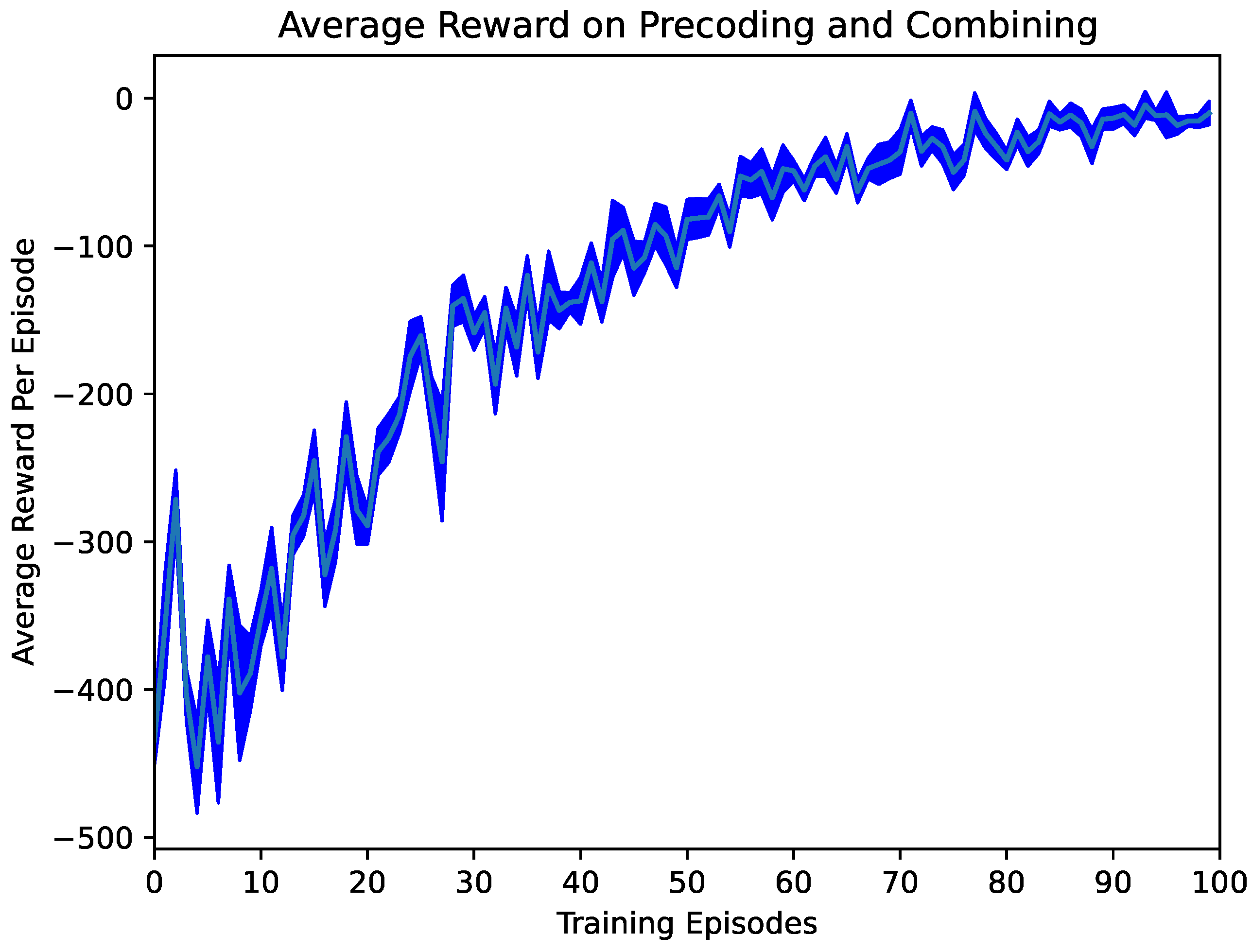
Figure 3 shows the average reward in the confidence interval for five runs to show statistical significance. As shown in Figure 3, the average reward converges with the number of training increases. This reward includes the optimization objective’s MSE and the penalty of constraint conditions. In the later stage of training, the penalty term is 0, and the entire reward represents MSE, which shows the effectiveness of our proposed scheme.
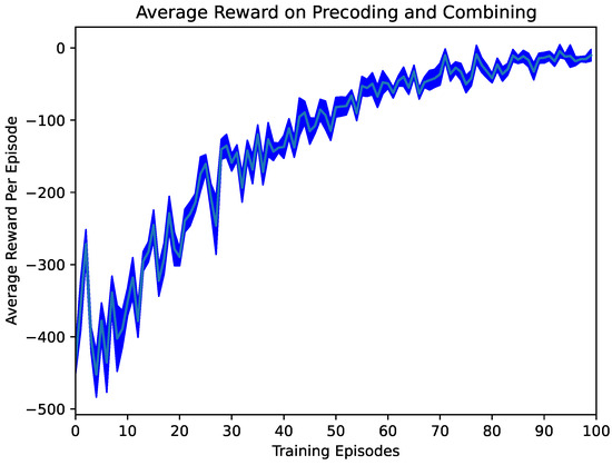
Figure 3.
Average reward of the proposed scheme.
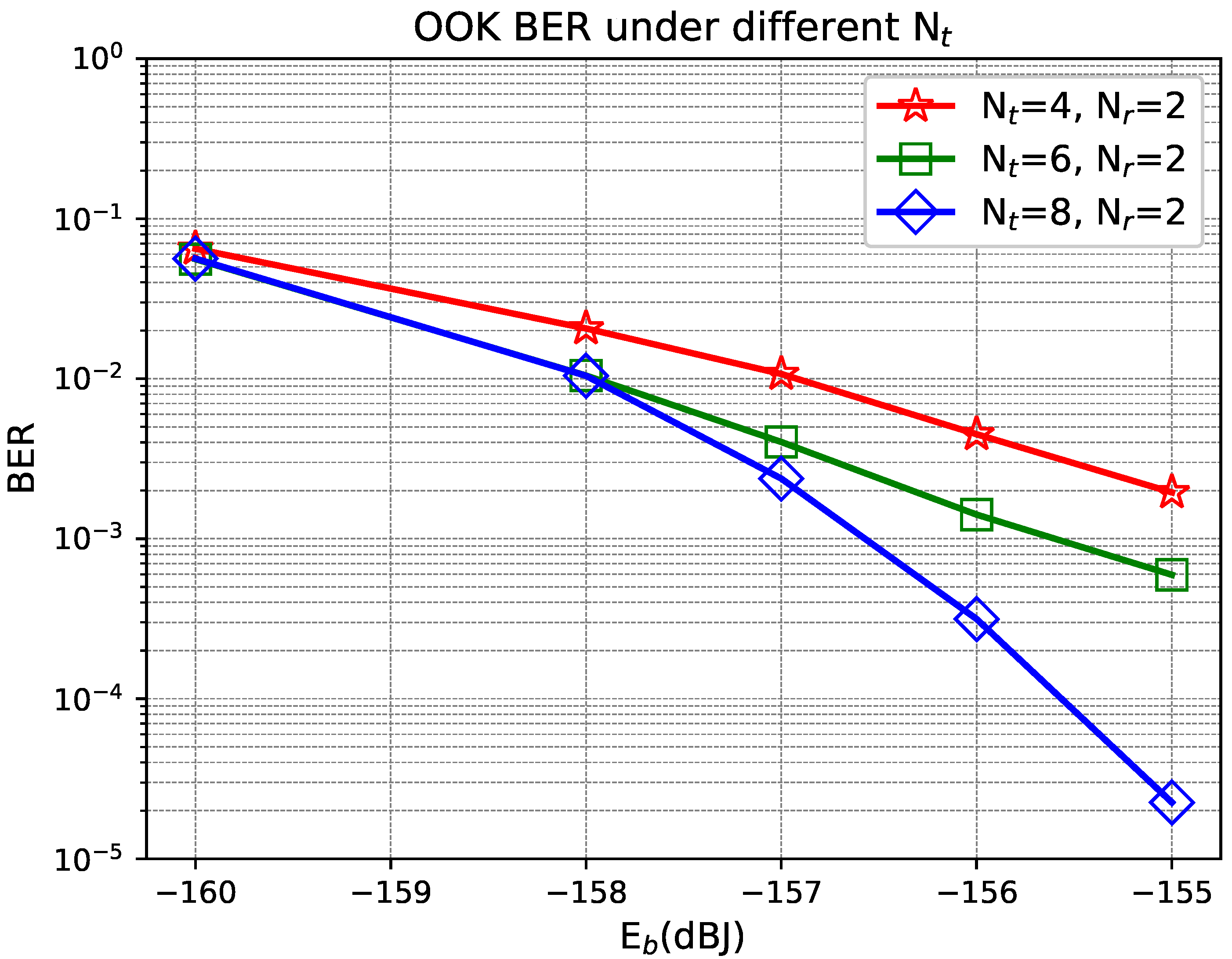
The impact of the number of LEDs is analyzed in Figure 4, where the background radiation is dBJ. The increase in the number of LED arrays () helps to reduce the BER. In particular, for a MIMO configuration, the proposed scheme achieves an average BER of at an energy per bit of dBJ, providing a performance gain of about 2 dB over the system. This indicates that the proposed scheme can efficiently utilize the spatial diversity. The result suggests that the proposed scheme can provide reliable and efficient data transmission even under low receive energy conditions.
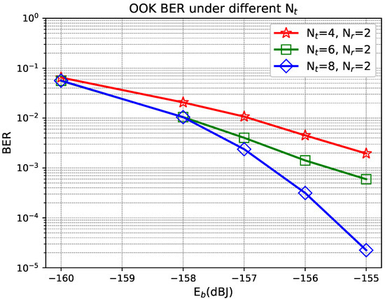
Figure 4.
Performance comparison under different with in strong turbulence.
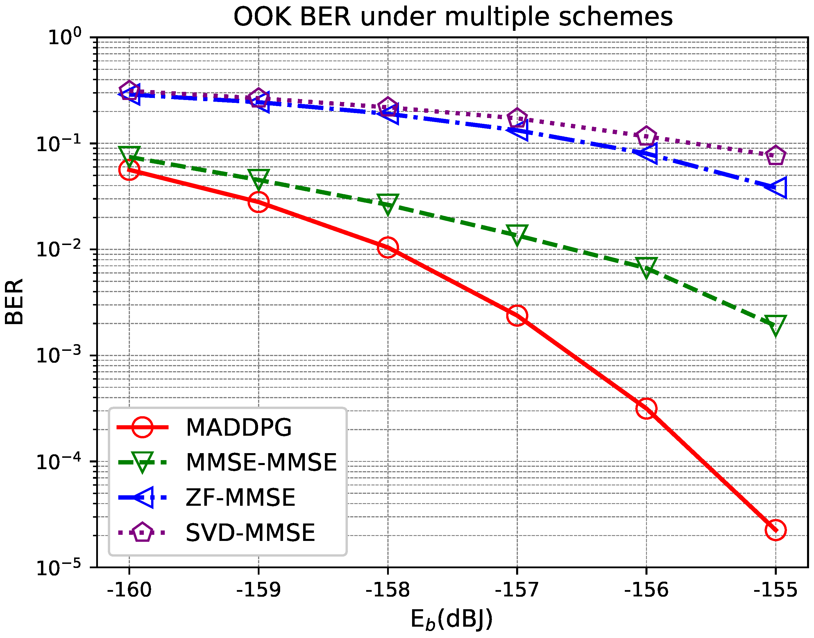
Figure 5 presents the performance comparison between our scheme and traditional AWGN-based precoding schemes in a severe fading channel with and . For traditional schemes, we considered different schemes at the receiver side and transmitted side [39,40,41]: MMSE-MMSE, ZF-MMSE, and SVD-MMSE. The background radiation is dBJ. It is clear that the AWGN-based MMSE precoding schemes perform poorly in the Poisson shot-noise photon-counting systems. The MMSE precoding scheme in the Gaussian system can only achieve a BER of when dBJ, while our proposed scheme can reach .
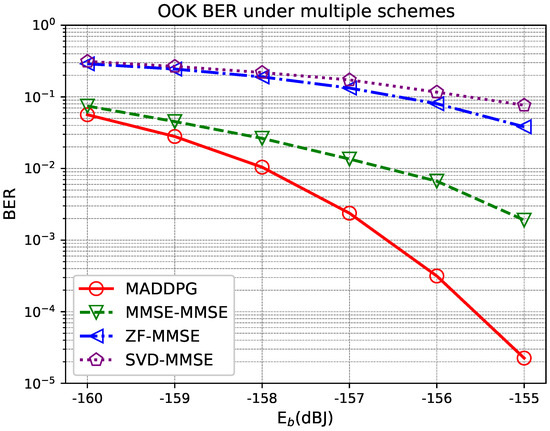
Figure 5.
Performance comparison with traditional Gaussian schemes for and in strong turbulence.
For the computational complexity analysis, we exploit the number of float number operations with Big-O notation. According to the formula, we can know that the computational complexity of the MMSE-MMSE, ZF-MMSE, and SVD-MMSE scheme is . Since the actor network of MADDPG uses the multi-layer perceptron structure, the computational complexity of the MADDPG generating precoding matrix and combining per execution for one agent is given by [42]:
where is the number of evaluation episodes; > , is the step number; L is the number of hidden layers; and is the nodes number of l-th hidden layer. for . Note that is a scaling factor, which depends on the dimension of states, for the hidden-layer nodes.
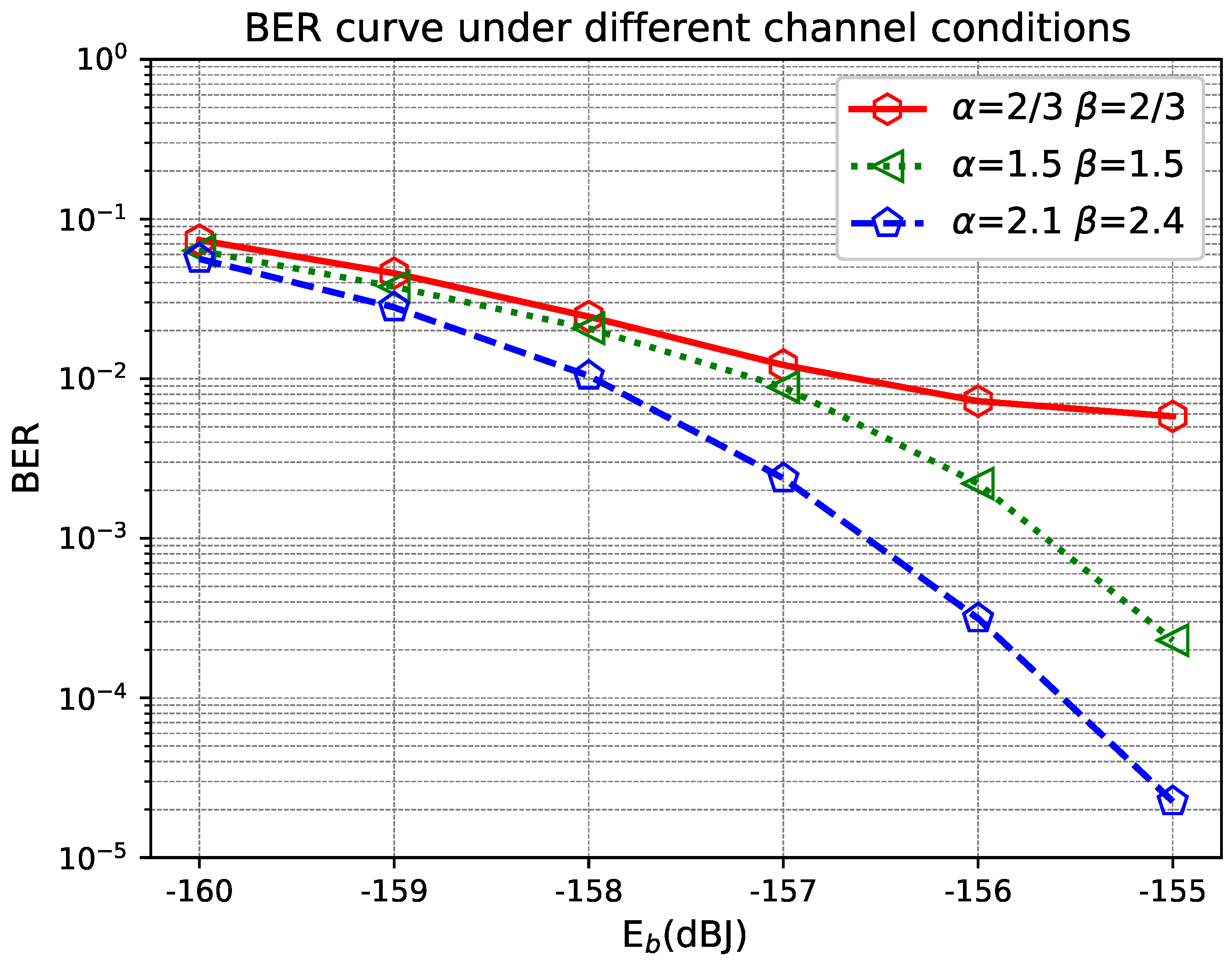
Figure 6 shows the BER of the proposed MMSE scheme under three different turbulence fading conditions, where and . It is observed that the proposed MMSE scheme could achieve a low BER as increases, under each of the turbulence fading conditions. However, under stronger turbulence, a higher is required to maintain the same BER target.

Figure 6.
Performance comparison under different turbulence channel.
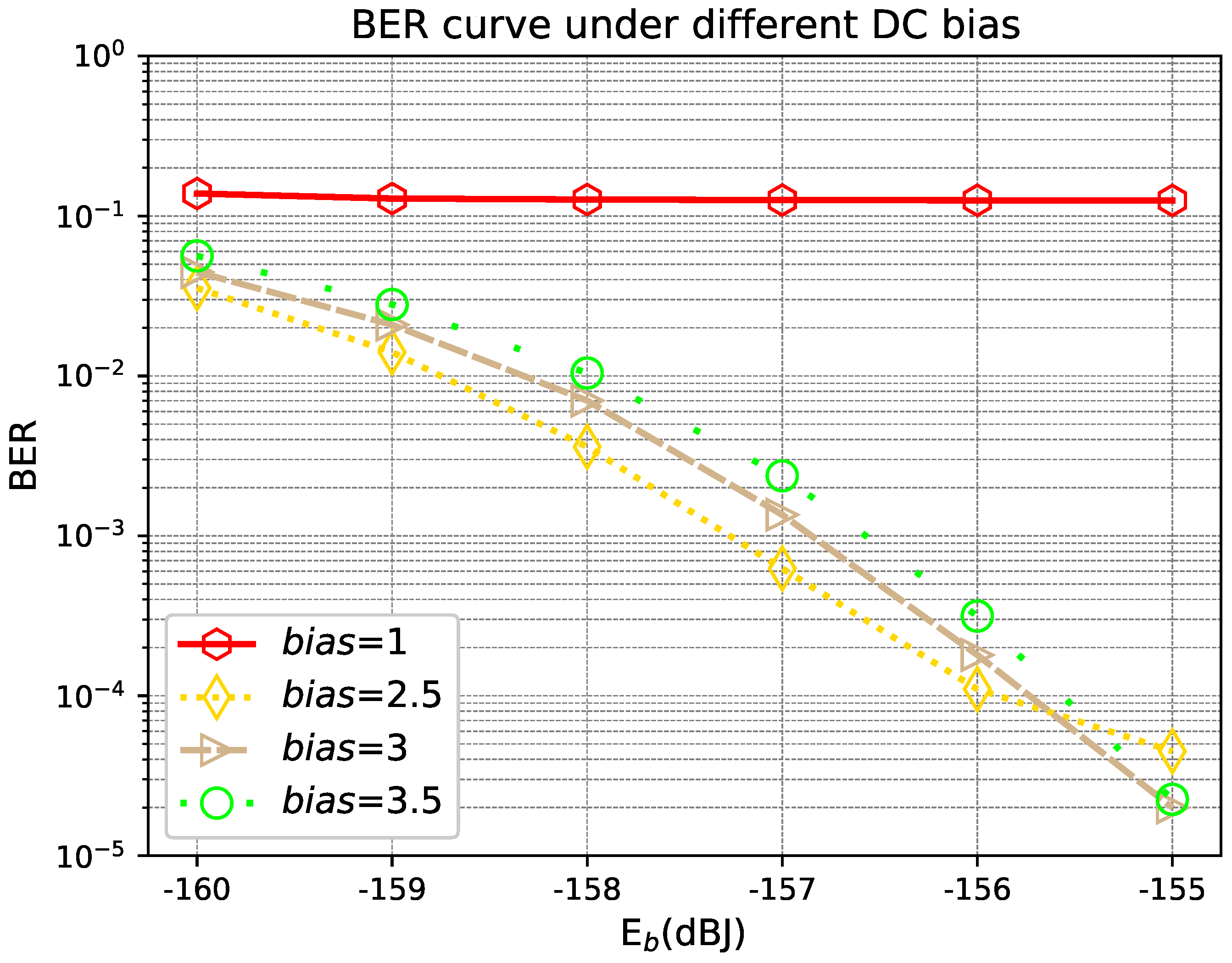
Figure 7 shows the BER performance of the proposed scheme with different DC bias. As shown in Figure 7, when the DC bias is 1, the BER cannot decrease. This is because the bias is too small to allow the LED to operate in a linear range. Compare the other three curves; it is obvious that a smaller DC bias tends to provide a better performance. This is because when the total power is given, the less the power is applied to biasing, the more power can be saved for transmitting useful signals.
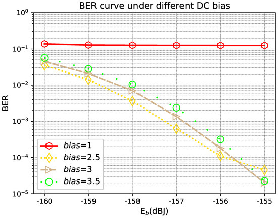
Figure 7.
Performance comparison under different DC biases in strong turbulence.
In FSO communication systems, CSI plays a critical role in designing and optimizing transmission schemes. However, CSI estimation errors can occur due to various factors, such as outdated or inaccurate feedback from the users. To investigate the BER performance of the proposed MIMO precoding scheme in the presence of imperfect CSI, the channel irradiance is modeled as , where the estimation error is independently and uniformly randomly distributed within the interval , and is the maximum error percentage. The CSI at the transmitter is modeled as a mapping , where is an arbitrary subset of .
To evaluate the robustness of the proposed MIMO precoding scheme, Figure 8 shows the BER performance in the presence of different levels of CSI imperfection in a strong gamma–gamma fading channel, where and . In Figure 8, the value of indicates perfect CSI, and it is observed that the proposed scheme is resilient to imperfect CSI. More specifically, it is clear that our scheme achieves a BER of or lower at dBJ even when the estimation error percentage is as high as . These results indicate the robustness of the proposed precoding scheme in practical communication systems.
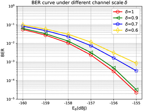
Figure 8.
Performance comparison under different types of CSI in strong turbulence.
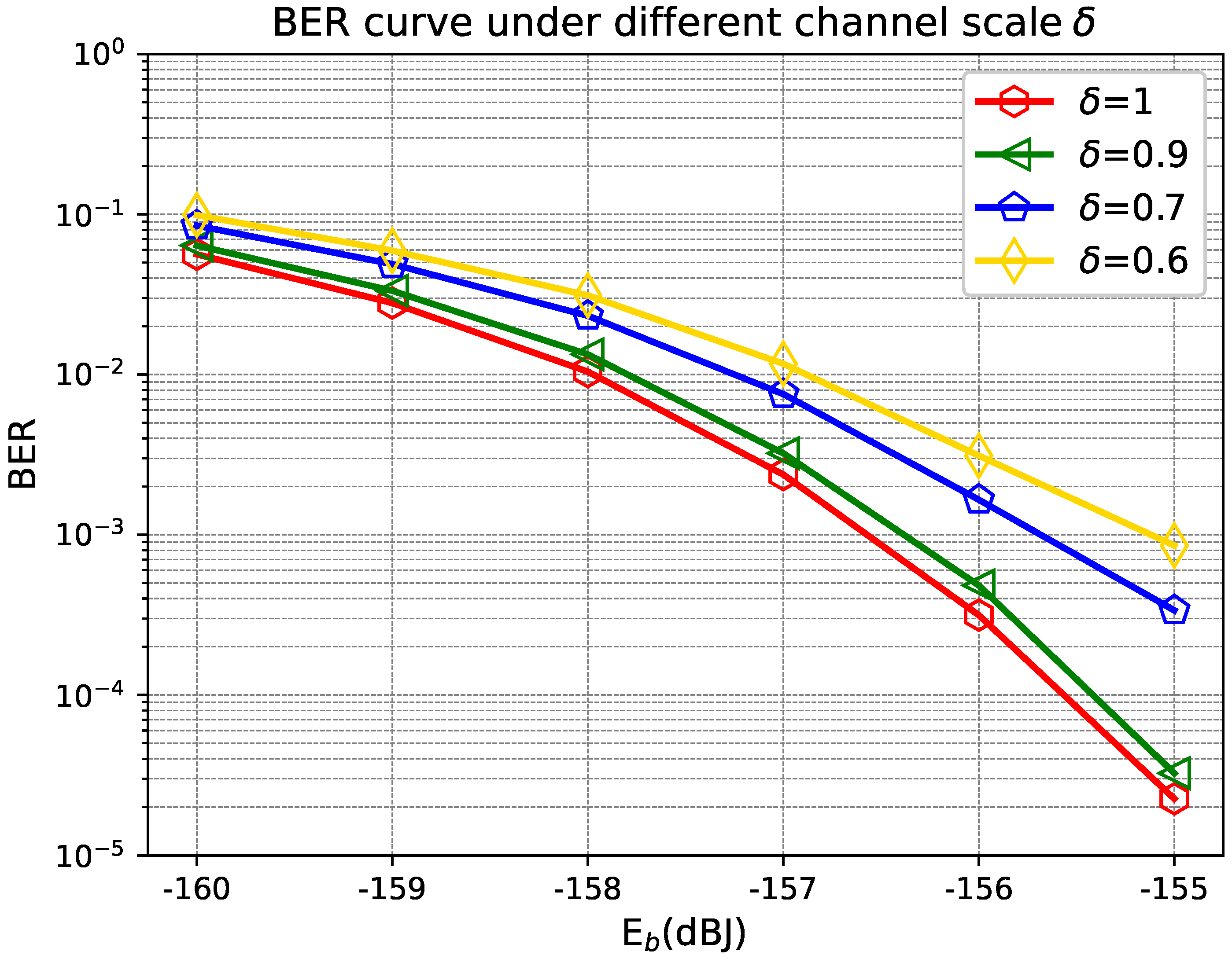
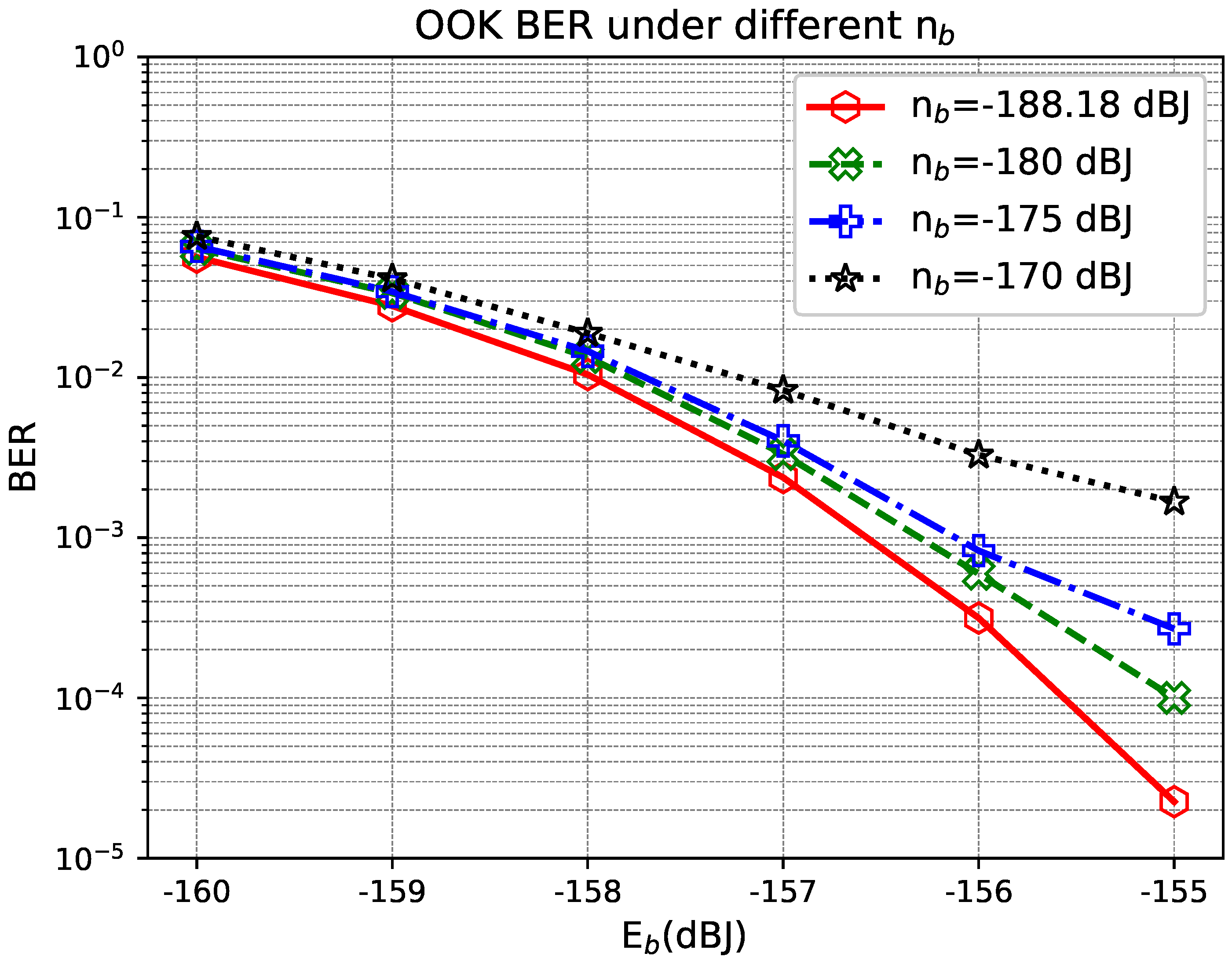
The background light intensity is a key factor affecting the performance of the FSO system. Figure 9 shows the system BER performance under different background light intensities (i.e., dBJ, dBJ, dBJ, and dBJ). It is clear that the proposed scheme can resist strong background light interference. Specifically, under the strong background light condition of dBJ, a BER can be achieved.
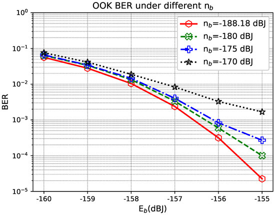
Figure 9.
Performance comparison under different in strong turbulence.
7. Conclusions
We presented a novel MIMO precoding scheme based on RL, jointly optimizing both the precoding and combining matrix of the transceiver and receiver, respectively. The simulation results indicate that the proposed RL-based MIMO precoding scheme outperforms existing methods under a wide range of operating conditions, delivering significant gains in terms of BER performance. The proposed system exhibits strong robustness and can achieve the BER of less than even when the CSI is imperfect. The proposed solution offers a highly effective approach for jointly optimizing both the precoding and detection matrix of the transceiver and receiver.
The dead time in photon counting systems refers to the minimum time delay that must occur between the detection of two consecutive photons by a detector. During this dead time period, the detector is unable to register or detect any subsequent photons. This study does not consider the impact of dead time. In the future, we can analyze the system throughput with precoding and the impact of dead time. In addition, the system considered in this article is a single user system, which can also be extended to multi-user systems in the future. It is worth exploring how to eliminate the inter-user interference in multi-user systems by designing precoding and detection matrices.
Author Contributions
Methodology, Z.L., C.W., and X.Z.; writing—original draft, Z.L. and C.W.; and writing—review and editing, X.Z., G.D., and Y.W. All authors have read and agreed to the published version of the manuscript.
Funding
This work was supported by the National Natural Science Foundation of China under Grant No. 62231010 and the Innovation Program of Shanghai Municipal Science and Technology Commission under Grant No. 21XD1400300.
Institutional Review Board Statement
Not applicable.
Informed Consent Statement
Not applicable.
Data Availability Statement
Not applicable.
Conflicts of Interest
The authors declare no conflict of interest.
Abbreviations
The following abbreviations are used in this manuscript:
| AWGN | Additive white Gaussian noise |
| IoT | Internet of Things |
| ADMM | Alternating directional multiplier method |
| MIMO | Multiple-input multiple-output |
| FSO | Free-space optical |
| BER | Bit error rate |
| CSI | Channel state information |
| NLOS | Non-line-of-sight |
| AI | Artificial intelligence |
| MMSE | Minimum mean square error |
| MADDPG | Multi-agent deep deterministic policy gradient |
| PPM | Pulse-position modulation |
| OOK | On–off keying |
| SPAD | Single-photon avalanche diode |
| NN | Neural network |
| HCE | Hybrid cross entropy |
| LED | Light-emitting diodes |
| DC | Direct current |
| PD | Photo detector |
Appendix A
Define a set with alphabet size , where each element of yields the same a priori probability . Based on (6), the conditional probability distribution of receiver i’s received signal given is provided by
Then, we have
It follows from (A2) that is the average of the expected values of Poisson random variables with means . Hence, we have
Note that , where is the j-th column of the identity matrix . Consequently, (A3) is equivalent to
Similarly, we can derive
References
- Huang, X.; Zhang, J.; Liu, R.; Guo, Y.; Hanzo, L. Airplane-aided integrated networking for 6G wireless: Will it work? IEEE Veh. Technol. Mag. 2019, 14, 84–91. [Google Scholar] [CrossRef]
- Khalighi, M.A.; Uysal, M. Survey on free space optical communication: A communication theory perspective. IEEE Commun. Surv. Tutor. 2014, 16, 2231–2258. [Google Scholar] [CrossRef]
- Al-Gailani, S.A.; Salleh, M.F.M.; Salem, A.A.; Shaddad, R.Q.; Sheikh, U.U.; Algeelani, N.A.; Almohamad, T.A. A survey of free space optics (FSO) communication systems, links, and networks. IEEE Access 2020, 9, 7353–7373. [Google Scholar] [CrossRef]
- Liu, B.; Gong, C.; Cheng, J.; Xu, Z. Correlation-based LTI channel estimation for multi-wavelength optical scattering NLOS communication. IEEE Trans. Commun. 2020, 68, 1648–1661. [Google Scholar] [CrossRef]
- Jiang, W.; Han, B.; Habibi, M.A.; Schotten, H.D. The road towards 6G: A comprehensive survey. IEEE Open J. Commun. Soc. 2021, 2, 334–366. [Google Scholar] [CrossRef]
- Zhang, M.; Gao, J.; Zhong, C. A deep learning-based framework for low complexity multiuser MIMO precoding design. IEEE Trans. Wireless Commun. 2022, 21, 11193–11206. [Google Scholar] [CrossRef]
- Kebede, T.; Wondie, Y.; Steinbrunn, J.; Kassa, H.B.; Kornegay, K.T. Precoding and beamforming techniques in mmWave-massive MIMO: Performance assessment. IEEE Access 2022, 10, 16365–16387. [Google Scholar] [CrossRef]
- Choi, J.; Park, J.; Lee, N. Energy efficiency maximization precoding for quantized massive MIMO systems. IEEE Trans. Wirel. Commun. 2022, 21, 6803–6817. [Google Scholar] [CrossRef]
- Guo, D.; Shamai, S.; Verdú, S. Mutual information and conditional mean estimation in Poisson channels. IEEE Trans. Inf. Theory 2008, 54, 1837–1849. [Google Scholar] [CrossRef]
- Ahmadypour, N.; Gohari, A. Transmission of a bit over a discrete Poisson channel with memory. IEEE Trans. Inf. Theory 2021, 67, 4710–4727. [Google Scholar] [CrossRef]
- Huang, C.; Mo, R.; Yuen, C. Reconfigurable intelligent surface assisted multiuser MISO systems exploiting deep reinforcement learning. IEEE J. Sel. Areas Commun. 2020, 38, 1839–1850. [Google Scholar] [CrossRef]
- Zhu, Y.; Bo, Z.; Li, M.; Liu, Y.; Liu, Q.; Chang, Z.; Hu, Y. Deep reinforcement learning based joint active and passive beamforming design for RIS-assisted MISO systems. In Proceedings of the 2022 IEEE Wireless Communications and Networking Conference (WCNC), Austin, TX, USA, 10–13 April 2022; pp. 477–482. [Google Scholar]
- Lee, H.; Girnyk, M.; Jeong, J. Deep reinforcement learning approach to MIMO precoding problem: Optimality and robustness. arXiv 2020, arXiv:2006.16646. [Google Scholar]
- Zhang, C.; Patras, P.; Haddadi, H. Deep learning in mobile and wireless networking: A survey. IEEE Commun. Surv. Tutor. 2019, 21, 2224–2287. [Google Scholar] [CrossRef]
- Luong, N.C.; Hoang, D.T.; Gong, S.; Niyato, D.; Wang, P.; Liang, Y.C.; Kim, D.I. Applications of deep reinforcement learning in communications and networking: A survey. IEEE Commun. Surv. Tutor. 2019, 21, 3133–3174. [Google Scholar] [CrossRef]
- Lowe, R.; Wu, Y.I.; Tamar, A.; Harb, J.; Pieter Abbeel, O.; Mordatch, I. Multi-agent actor–critic for mixed cooperative-competitive environments. In Proceedings of the 31st International Conference on Neural Information Processing Systems, Long Beach, CA, USA, 4–9 December 2017; pp. 6382–6393. [Google Scholar]
- Abou-Rjeily, C. Spatial multiplexing for photon-counting MIMO-FSO communication systems. IEEE Trans. Wirel. Commun. 2018, 17, 5789–5803. [Google Scholar] [CrossRef]
- Gong, C.; Xu, Z. LMMSE SIMO receiver for short-range non-line-of-sight scattering communication. IEEE Trans. Wirel. Commun. 2015, 14, 5338–5349. [Google Scholar] [CrossRef]
- Sharifzadeh, M.; Ahmadirad, M. Performance analysis of underwater wireless optical communication systems over a wide range of optical turbulence. Opt. Commun. 2018, 427, 609–616. [Google Scholar] [CrossRef]
- Zhou, X.; Wei, C.; Shen, D.; Xu, C.; Wang, L.; Yu, X. A shot noise limited quantum iterative massive MIMO system over Poisson atmospheric channels. In Proceedings of the 2019 IEEE International Conference on Communications (ICC), Shanghai, China, 20–24 May 2019; pp. 1–6. [Google Scholar]
- Wang, S.; Peng, M.; Yuan, R. MIMO free-space optical communications using photon-counting receivers under weak links. IEEE Commun. Lett. 2023, 27, 1185–1189. [Google Scholar] [CrossRef]
- Gong, C.; Xu, Z. Non-line of sight optical wireless relaying with the photon counting receiver: A count-and-forward protocol. IEEE Trans. Wirel. Commun. 2014, 14, 376–388. [Google Scholar] [CrossRef]
- Etemadi, A.; Arjmandi, H.; Azmi, P.; Mokari, N. Capacity bounds for diffusive molecular communication over discrete-time compound Poisson channels. IEEE Commun. Lett. 2019, 23, 793–796. [Google Scholar] [CrossRef]
- Sarbazi, E.; Safari, M.; Haas, H. The bit error performance and information transfer rate of SPAD array optical receivers. IEEE Trans. Commun. 2020, 68, 5689–5705. [Google Scholar] [CrossRef]
- Zhang, Y.; Huo, Y.; Zhan, J.; Wang, D.; Dong, X.; You, X. ADMM enabled hybrid precoding in wideband distributed phased arrays based MIMO systems. In Proceedings of the 2019 IEEE 90th Vehicular Technology Conference (VTC2019-Fall), Honolulu, HI, USA, 22–25 September 2019; pp. 1–5. [Google Scholar]
- Chen, C.E. Symbol-level precoding for multiuser multiple-input-single-output downlink systems with low-resolution DACs. IEEE Trans. Veh. Technol. 2021, 71, 2116–2121. [Google Scholar] [CrossRef]
- Xu, W.; Wang, Y.; Xue, X. ADMM for hybrid precoding of relay in millimeter-wave massive MIMO system. In Proceedings of the 2018 IEEE 88th Vehicular Technology Conference (VTC-Fall), Chicago, IL, USA, 27–30 August 2018; pp. 1–5. [Google Scholar]
- Li, X.; Dang, J.; Zhang, Z. ADMM based symbol-level precoding for MU-MISO downlink with low-resolution DACs. IEEE Commun. Lett. 2022, 26, 2974–2978. [Google Scholar] [CrossRef]
- Raptis, N.; Pikasis, E.; Syvridis, D. Power losses in diffuse ultraviolet optical communications channels. Opt. Lett. 2016, 41, 4421–4424. [Google Scholar] [CrossRef] [PubMed]
- Meng, X.; Zhang, M.; Han, D.; Song, L.; Luo, P. Experimental study on 1× 4 real-time SIMO diversity reception scheme for a ultraviolet communication system. In Proceedings of the 2015 20th European Conference on Networks and Optical Communications (NOC), London, UK, 30 June–2 July 2015; pp. 1–4. [Google Scholar]
- Zhao, T.; Yao, J.; Gong, C.; Wang, Y. Wireless ultraviolet light MIMO assisted UAV direction perception and collision avoidance method. Phys. Commun. 2022, 54, 101815. [Google Scholar] [CrossRef]
- Hasan Hariq, S.; Odabasioglu, N. Spatial diversity techniques for non-line-of-sight ultraviolet communication systems over atmospheric turbulence channels. IET Optoelectron. 2020, 14, 327–336. [Google Scholar] [CrossRef]
- Ding, T.; Zhao, Y.; Li, L.; Hu, D.; Zhang, L. Hybrid precoding for beamspace MIMO systems with sub-connected switches: A machine learning approach. IEEE Access 2019, 7, 143273–143281. [Google Scholar] [CrossRef]
- Hu, Q.; Liu, Y.; Cai, Y.; Yu, G.; Ding, Z. Joint deep reinforcement learning and unfolding: Beam selection and precoding for mmWave multiuser MIMO with lens arrays. IEEE J. Sel. Areas Commun. 2021, 39, 2289–2304. [Google Scholar] [CrossRef]
- Ahmed, I.; Shahid, M.K.; Faisal, T. Deep reinforcement learning based beam selection for hybrid beamforming and user grouping in massive MIMO-NOMA system. IEEE Access 2022, 10, 89519–89533. [Google Scholar] [CrossRef]
- Zhao, L.; Cai, K.; Jiang, M. Multiuser precoded MIMO visible light communication systems enabling spatial dimming. J. Light. Technol. 2020, 38, 5624–5634. [Google Scholar] [CrossRef]
- Fredj, F.; Al-Eryani, Y.; Maghsudi, S.; Akrout, M.; Hossain, E. Distributed uplink beamforming in cell-free networks using deep reinforcement learning. arXiv 2020, arXiv:2006.15138. [Google Scholar]
- Wang, G.; Gong, C.; Xu, Z. Signal characterization for multiple access non-line of sight scattering communication. IEEE Trans. Commun. 2018, 66, 4138–4154. [Google Scholar] [CrossRef]
- Mustafa, H.M.T.; Baik, J.-I.; You, Y.-H.; Song, H.-K.; Abbasi, Z. Hybrid beamforming and relay selection for end-to-end SNR maximization in single-user multi-relay MIMO systems. Sensors 2023, 23, 2079. [Google Scholar] [CrossRef] [PubMed]
- Fang, S.; Huang, R.; Xiao, Y.; Zhu, P.; Xie, J.; Zhang, S.; Miao, J. Zero forcing assisted single layer beamforming for spatial modulation MIMO systems. IEEE Trans. Veh. Technol. 2022, 71, 4116–4128. [Google Scholar] [CrossRef]
- Chen, C.E. Constructive interference-based symbol-level precoding for generalized precoding-aided spatial modulation with PSK signaling. IEEE Commun. Lett. 2020, 24, 1816–1820. [Google Scholar] [CrossRef]
- Kim, H.; Choi, J.; Love, D.J. Massive MIMO Channel Prediction Via Meta-Learning and Deep Denoising: Is a Small Dataset Enough? IEEE Trans. Wirel. Commun. 2023. early access. [Google Scholar] [CrossRef]
Disclaimer/Publisher’s Note: The statements, opinions and data contained in all publications are solely those of the individual author(s) and contributor(s) and not of MDPI and/or the editor(s). MDPI and/or the editor(s) disclaim responsibility for any injury to people or property resulting from any ideas, methods, instructions or products referred to in the content. |
© 2023 by the authors. Licensee MDPI, Basel, Switzerland. This article is an open access article distributed under the terms and conditions of the Creative Commons Attribution (CC BY) license (https://creativecommons.org/licenses/by/4.0/).