Dynamic Optimization of Mechanism Parameters of Bipedal Robot Considering Full-Range Walking Energy Efficiency

Abstract

Mechanism parameters of bipedal robots are crucial for achieving efficient locomotion in complex environments. Inspired by the human energy-efficient walking style, this paper proposes a novel concept of full-range walking energy efficiency and explores the optimal linkage mechanism within certain ranges of step length and walking speed for bipedal robots. First, a bipedal model incorporating an upper body is established for dynamic analysis. Next, an optimal walking gait subject to walking constraints is solved by considering the full-range energy efficiency. Further, an optimal linkage mechanism is investigated, and the influence of dynamic parameters on energy efficiency is analyzed. Finally, the push-off impulse, minimum ground support force, and walking torque features are discussed. It shows that the full-range walking energy efficiency can be lowered by reducing the ratio of leg mass, concentrating mass at the hip joint, decreasing the length of the upper body, or increasing the center of mass of the leg. In addition, efficient walking motion can be achieved by designing the coordination of positive hip joint torque and push-off impulse at the ankle. This paper can be used to guide the mechanism parameter optimization and efficient walking gait design of bipedal robots.

1. Introduction

Bipedal robot technologies are crucial for the advancement of science and technology. Compared with other types of robots with wheels [1,2], tracks [3], or multiple legs [4], bipedal robots possess superior adaptability and flexibility in complex terrains. With a body structure resembling that of humans, bipedal robots are well-suited to adapt to human living and working environments [5]. They can engage in tasks alongside humans or collaborate with them [6], for example, in operating production stations, assisting in driving, conducting rescue operations in hazardous areas [7,8], and navigating human environments, including stairs and obstacles. Humanoid bipedal robots are expected to emerge as a prominent robot form in the future. However, the realization of efficient walking in complex ground environments remains a challenge within the bipedal robotics field.

Research on gait planning for bipedal robots has a history of more than 50 years, with varying degrees of accomplishments globally. In 2020, Boston Dynamics in the United States unveiled the latest version of their bipedal robot, Atlas, which showcased impressive walking capabilities using hydraulic actuation technologies. This robot can walk stably on uneven terrains and also execute complex movements such as jumping and dancing [9]. Other well-known bipedal robots have also demonstrated remarkable walking performance. For instance, the German Aerospace Center’s TORO robot (2013) features full-torque control [10], NASA’s Valkyrie bipedal robot (2013) can operate in degraded or damaged human-engineered environments [11], Toyota’s T-HR3 robot (2017) exhibits teleoperation capabilities [12], the HRP-5P robot developed by Japan’s AIST (2018) [13] can perform autonomous heavy labor in hazardous settings, and the UBTECH Walker (2019) developed in China can provide bipedal robot services for everyday tasks [14]. In terms of research on bipedal robot walking motion control, Tedrake (2016) successfully achieved stable walking motion for the Atlas robot by using a simplified dynamic model trajectory based on the time-varying linear quadratic regulator (LQR). This method compares the cost of the optimal LQR with that associated with quadratic programming, based on the robot’s instantaneous dynamics, input signals, and constraints [15].

Kim (2018) simplified robot dynamics into a convex optimization problem and used model predictive control (MPC) to estimate the ground reaction force, thereby achieving fast and stable walking for the Cheetah robot [16]. Notably, the abovementioned robots use advanced control algorithms, such as MPC and LQR, for real-time control of their joints to achieve stable walking motion. However, compared with humans, the walking movement of robots lacks natural and smooth characteristics, and the energy consumed during walking is significantly higher. Specifically, the walking energy efficiency index, known as the cost of transport ($COT$), is typically several times higher for robots than that for humans [17].

To address the challenges encountered by bipedal robots, a promising strategy is to use a gait that mimics human walking as the starting point and then improve the leg mechanism design. In 2022, Boston Dynamics released Atlas, a high-performance robot driven by hydraulics. The leg mechanism of this robot has a multi-degree-of-freedom serial structure, offering excellent flexibility and load-bearing walking capability. Nevertheless, it faces several issues such as insufficient battery life and limited movement speed [9]. Furthermore, robots using electric drive joints have also demonstrated impressive performance. Germany’s DLR introduced the TORO bipedal robot in 2013, which can exhibit smooth and efficient walking in various complex environments via compliant torque control [10]. The StarlETH robot designed by Hutter in 2012 employs a chain drive for lower leg motion [18]. Alexander presented the design of the Cheetah robot in 2013, using a rope drive for the knee joint [19]. Additionally, Seok, in 2013, developed a high-speed Cheetah robot that uses a connecting rod transmission and four-bar mechanism to drive lower leg movement [20]. In 2022, Hurst developed a Cassie bipedal robot that emulates the characteristics of an ostrich. This robot features an efficient four-link series leg structure, enabling it to perform tasks in various complex environments [21]. Another notable creation is the Tesla Bot (Optimus), a humanoid robot equipped with electromechanical push rods, designed to undertake dangerous or repetitive tasks [22]. Grizzle (2013) introduced the MABEL bipedal robot, inspired by human leg bionics. Its mechanical structure imitates human bones and muscles, with most of the weight concentrated in the upper body, resulting in lighter legs capable of swift forward and backward movement [23]. Valkyrie, a humanoid robot developed by NASA in the United States (2013), incorporates anthropometry and biomechanics. Its legs involve a series of elastic brakes, enabling torque control and providing walking, balance, and manipulation capabilities [24]. Xie (2020) implemented a bionic design of bipedal robot mechanical legs based on human biodynamic models, simulating human walking gaits [25]. Zhao (2023) developed an electro-hydraulic hybrid drive system for bipedal robots that aligns with human walking functions. This type of bipedal robot is designed based on bionics principles and can achieve natural and stable walking gaits via optimized mechanisms while reducing the unit energy consumption during walking [26].

Once the mechanism design is finalized, the optimization of mechanistic parameters becomes a key research focus for enhancing the performance and efficiency of bipedal robots. In recent years, scholars have actively conducted research in this realm. Chebbi (2020) introduced a novel algorithm that combines the genetic algorithm and Krawczyk operator. The aim is to minimize the robot’s position error while ensuring maximum tolerance of the design parameters [27]. To enhance flexibility and reduce energy consumption, Wu (2020) proposed an integrated approach utilizing the niche Pareto genetic algorithm to optimize the size and joint angles of multi-link robots, providing a fresh perspective on the dimension synthesis of such robots [28]. Kavala (2022) used three algorithms based on population optimization, specifically genetic algorithms, particle swarm optimization, and differential evolution techniques, to realize the structural design and controller optimization of five-bar planar manipulators. Different optimization methods exhibited distinct characteristics across various optimization problems [29]. Li (2021) proposed a six-bar linkage mechanism, featuring a natural ankle trajectory. Additionally, the researchers proposed a collaborative dual particle swarm optimization algorithm to enhance the structural design parameters [30]. Gao (2021) proposed a bionic knee joint exoskeleton structure utilizing a cross-based four-bar linkage mechanism. The particle swarm optimization algorithm was implemented to optimize the dimensions and placement of the structure, enabling it to mimic human knee joint motion [31]. Notably, the existing research has been primarily focused on ensuring stability performance, and further improvement is still needed to optimize the mechanism and parameters of bipedal robots. In the case of bipedal robots, the objective is to continuously optimize energy consumption by drawing insights from human walking motions and imitating human walking methods [32,33]. By considering the energy consumption across the complete range of walking steps and speeds, valuable insights can be derived for designing and optimizing the mechanisms and parameters of robots.

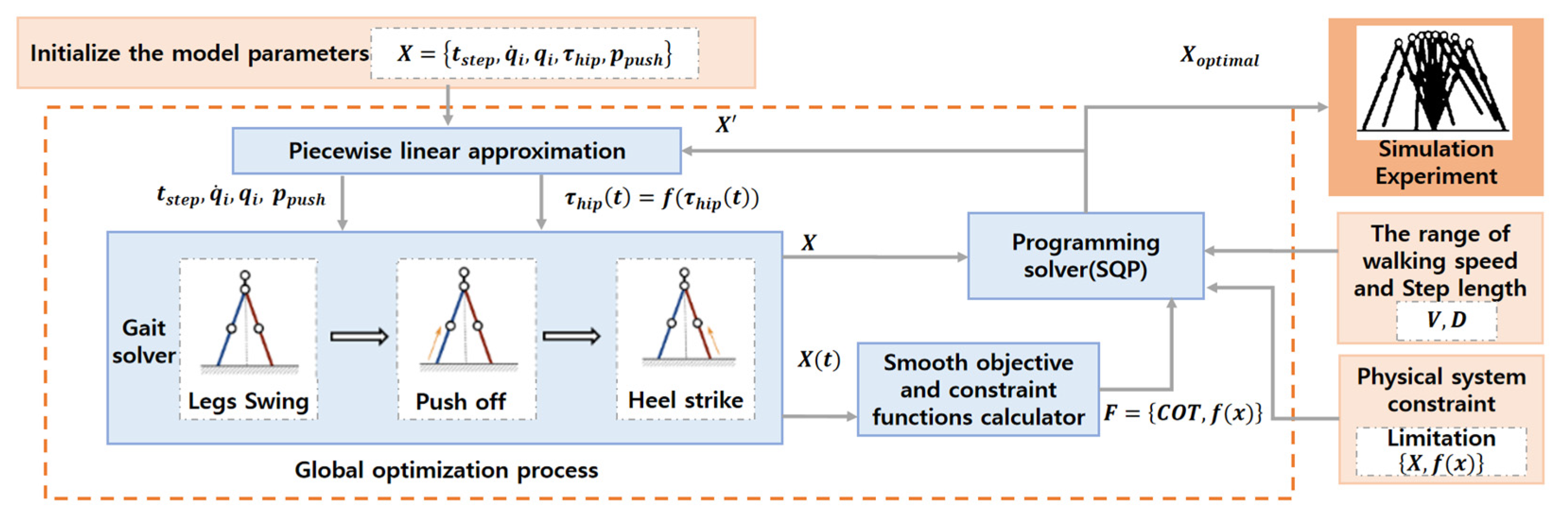
Therefore, this paper first established a dynamic parameter optimization model for bipedal robots based on full-range walking energy efficiency to analyze the dynamics of the robot. Next, the optimal mechanism parameters subject to constraints related to walking gait and environmental variables are solved. Then, the optimal linkage mechanism for the bipedal robot is investigated, and the influence of robot dynamic parameters on walking energy efficiency is analyzed. Finally, the gait characteristics of bipedal robots during walking are analyzed.

The arrangement of the paper is as follows: Section 2 presents the analysis of the walking motion. Section 3 addresses the energy optimal control problem. Section 4 discusses the conclusions drawn from specific experiments and the findings. Section 5 provides a summary of the aforementioned conclusions.

The main contribution of this paper is to propose a method for optimizing the dynamic parameters of bipedal robots based on full-range walking energy efficiency. By analyzing the impact of dynamic parameters on full-range energy consumption, the optimal mechanism and walking gait for bipedal robots are determined.

2. Analysis of the Gait Pattern

2.1. Model Analysis

The proposed model comprises two symmetrical rigid rod-like legs and an upper body. As shown in Figure 1, the upper body is reduced to a mass point with a mass of $m_{\mathrm{b}}$. The hip joint of the robot is located at a distance of $l_{\mathrm{b}}$ from the upper body mass point, and the mass attributed to the hip joint is denoted by $m_{\mathrm{h}}$. The hip joint serves as a hinge connecting the two legs, and the leg length is denoted as l. The length of the thigh and shin is, respectively, defined as $l_{\mathrm{t}\mathrm{h}}$ and $l_{\mathrm{s}\mathrm{h}}$, and the mass of each leg is denoted by $m_{\mathrm{l}}$. $q_1$ represents the angle of the stance leg relative to the normal ground surface, and $q_2$ represents the angle between the swing leg and the stance leg, $q_{\mathrm{b}}$ represents the angle between the upper body and the ground surface normal. During the walking process, the upper body is designed to be on the line of the angle bisector between the two legs, and the counterclockwise direction is positive. The relationship between $q_{\mathrm{b}}$ and $q_1, q_2$ is expressed as Equation (1):

$$q_{\mathrm{b}}= q_1+\frac{q_2}{2}$$

(1)

During the walking process, V represents the walking speed and D represents the step length. The torque in the model in this paper includes two components: the hip torque and the ankle torque. The combination of torque and push-off impulse supplies the necessary energy for the walking motion of the bipedal robot. The model is defined as a four DOFs system in a generalized coordinate system $q={\left[q_1{,q}_2{,x}_0{,y}_0\right]}^T,\left(q_1{,q}_2\right)$, represented as robot joint angles,$\mathrm{w}\mathrm{h}\mathrm{e}\mathrm{r}\mathrm{e}\left(x_0,y_0\right)$ denotes the coordinates of the stance foot in the Cartesian coordinate system, with the positive direction to the right, and the initial coordinates of the stance foot are set to $\left(\mathrm{0,0}\right)$.

2.2. Walking Motion

As shown in Figure 1, taking the flat ground as an example, the whole walking step cycle includes two phases, which are the swing phase of the swing leg and the heel-strike phase. The swing phase commences when both legs are in contact with the ground simultaneously, and then the swing leg starts to swing and leaves the ground. The swing phase concludes upon contact of the swing leg with the ground. Subsequently, the stance leg applies an instantaneous push-off force, followed by the heel-strike of the swing leg. A full cycle of walking motion is completed and the same initial state of the next cycle is set.

From the perspective of dynamics, it is necessary to consider the stage of the heel-strike during the transition from the stance phase to the swing phase of the robot, this moment creates an instantaneous push-off impulse $p_{\mathrm{p}\mathrm{u}\mathrm{s}\mathrm{h}}$, which can change the dynamic model of a bipedal robot. This paper assumes that when the swing leg makes contact with the ground, and the actions of push-off, heel-strike, and bipedal support occur sequentially as instantaneous events. In this section, the analysis focuses solely on the perspective of heel-strike. At the moment of heel-strike, the bipedal robot transitions from its continuous state to a discrete state and moves on to the next gait cycle.

In this paper, we made the assumption that there is no bouncing process during the heel-strike and the swing phase, and that only the stance foot remains in contact with the ground. By imposing constraints on the state of the stance foot, the constrained force between the ground and the stance foot can be found. These forces include frictional force along the slope direction and ground support force normal to the slope direction. Using calculations, we were able to test whether the stance foot satisfied the constrained friction coefficient and whether it became airborne.

2.3. Robot Dynamics Description

After simplifying the bipedal robot to a bipedal robot model, it is necessary to apply joint torques to the robot throughout its entire motion space to control the joints to move along the specified trajectory, in order to facilitate the control of the robot’s walking gait.

In this section, the dynamic analysis of the bipedal robot is performed utilizing the Lagrange equations, aiming to explore optimal energy efficiency. The variations in the system’s kinetic and potential energy are elucidated via the application of the principle of energy conservation. Dynamic analysis serves as a fundamental framework for energy optimization, and the utilization of mathematical modeling to analyze energy conversion has demonstrated successful applications in other fields [34,35].

The Lagrangian function is defined as Equation (2):

$$L\left(q,\ddot{q}\right)=E-K$$

(2)

where $L$ represents the Lagrange equation, and $\mathrm{q}$ represents the generalized coordinates in a dynamic system. $E$ and $K$ are the system’s kinetic and potential energies, respectively, both of which are functions of $q$; the system’s dynamics can be shown as Equation (3):

$$\frac{d}{dt}\left(\frac{\partial L}{\partial \dot{q}}\right)-\frac{\partial L}{\partial q}=J^{T}u$$

(3)

Kinetic Analysis

• Swing phase:

The relationship between the links is derived, and the total vector $X_{\mathrm{w}}$ of the robot walking model can be shown as Equation (4):

$$X_w=\left[\begin{array}{c}\begin{array}{c}{x}_{st}\\ y_{st}\\ x_{hip}\end{array}\\ \begin{array}{c}{y}_{hip}\\ x_b\end{array}\\ \begin{array}{c}{y}_b\\ x_{sw}\\ y_{sw}\end{array}\end{array}\right]=\left[\begin{array}{c}\begin{array}{c}{x}_0-l_{sh}\mathit{sin}\left(q_1\right)\\ y_0+l_{sh}\mathit{cos}\left(q_1\right)\\ x_0-l\mathit{sin}\left(q_1\right)\end{array}\\ y_0+l\mathit{cos}\left(q_1\right)\\ \begin{array}{c}{x}_0-l\mathit{sin}\left(q_1\right)-l_b\mathit{sin}\left(q_1+\frac{q_2}{2}\right)\\ y_0+l\mathit{cos}\left(q_1\right)+l_b\mathit{cos}\left(q_1+\frac{q_2}{2}\right)\\ \begin{array}{c}{x}_0-l\mathit{sin}\left(q_1\right)+l_{th}\mathit{sin}\left(q_1+q_2\right)\\ y_0+l\mathit{cos}\left(q_1\right)-l_{th}\mathit{cos}\left(q_1+q_2\right)\end{array}\end{array}\end{array}\right]$$

(4)

The energy (kinetic energy $E$ and potential energy $K$) of the bipedal robot can be shown as Equations (5)–(10):

$$\begin{gathered} E=\frac{1}{2}\left[m_b\left({\dot{x_b}}^2+{\dot{y_b}}^2\right)+m_h\left({\dot{x}}_{hip}^2+{\dot{y}}_{hip}^2\right)+m_l\left({\dot{x}}_{st}^2+{\dot{y}}_{st}^2\right) \\ +m_l\left({\dot{x}}_{sw}^2+{\dot{y}}_{sw}^2\right)\right] \end{gathered}$$

(5)

$$K=K_b+K_h+K_{st}+K_{sw}$$

(6)

$$K_b=m_{b}g\left(y_0+l\cos \left(q_1\right)-l_{th}\cos \left(q_1+q_2\right)\right)$$

(7)

$$K_h=m_{h}g\left(y_0+l\mathit{cos}\left(q_1\right)\right)$$

(8)

$$K_{st}=m_{l}g\left(y_0+l_{sh}\mathit{sin}\left(q_1\right)\right)$$

(9)

$$K_{sw}=m_{l}g\left(y_0+l\mathit{cos}\left(q_1\right)-l_{th}\mathit{cos}\left(q_1+q_2\right)\right)$$

(10)

Combining with Equation (4), the equation for the swing phase can be shown as Equation (11):

$$M\left(q\right)\ddot{q}+C\left(q,\dot{q}\right)\dot{q}+G\left(q\right)=J_r^{T}u+T$$

(11)

where $M\left(q\right)$ is the 4 × 4 matrix of $\ddot{q}$, $C\left(q,\dot{q}\right)\dot{q}$ and $G\left(q\right)$ are both 4 × 1 matrices, $J_r^{T}u$ is the constraint force of the stance foot, including the support force $u_{\mathrm{N}}$ and friction force $u_{\mathrm{N}}$, and $T$ is the joint torque, shown as Equations (12)–(16):

$$\mathrm{u}={\left[u_f,u_N\right]}^T$$

(12)

$$M(q)=\left[\begin{array}{llll}{M}_{11}\hfill & M_{12}\hfill & M_{13}\hfill & M_{14}\hfill \\ M_{21}\hfill & M_{22}\hfill & M_{23}\hfill & M_{24}\hfill \\ M_{31}\hfill & M_{32}\hfill & M_{33}\hfill & M_{34}\hfill \\ M_{41}\hfill & M_{41}\hfill & M_{43}\hfill & M_{44}\hfill \end{array}\right]$$

(13)

$$C(q,\dot{q})\dot{q}=\left[\begin{array}{c}{C}_1\\ C_2\\ C_3\\ C_4\end{array}\right]$$

(14)

$$G(q)=\left[\begin{array}{l}{G}_1\hfill \\ G_2\hfill \\ G_3\hfill \\ G_4\hfill \end{array}\right]$$

(15)

$$T={\left[0,{\tau }_{\mathrm{hip} },0,0\right]}^T$$

(16)

where the representations of $M$ and $C$ are shown as Equations (17)–(32):

$$M_{11}=2l_{sh}^2{m}_l+l_{sh}^2{m}_h+l_{th}^2{m}_h+4l_{th}^2{m}_l\sin {\left(q_2/2\right)}^2+2l_{sh}{l}_{th}{m}_h+4l_{sh}{l}_{th}{m}_l\sin {\left(q_2/2\right)}^2$$

(17)

$$M_{12}=M_{21}=-l_{th}{m}_l\left(l_{sh}\cos \left(q_2\right)-l_{th}+l_{th}\cos \left(q_2\right)\right)$$

(18)

$$\begin{array}{c}{M}_{13}=M_{31}=l_{th}{m}_l\cos \left(q_1+q_2\right)-l_{th}{m}_l\cos \left(q_1\right)-l_{sh}{m}_h\cos \left(q_1\right)\\ -l_{th}{m}_h\cos \left(q_1\right)-2l_{sh}{m}_l\cos \left(q_1\right)\end{array}$$

(19)

$$\begin{array}{cc}{M}_{14}& =M_{41}=l_{th}{m}_i\sin (q_1+q_2)-l_{th}{m}_i\sin (q_1)-l_{sh}{m}_h\sin (q_1)\\ & -l_{th}{m}_h\sin (q_1)-2l_{sh}{m}_i\sin (q_1)\end{array}$$

(20)

$$M_{23}=M_{32}=l_{th}{m}_l\cos (q_1+q_2)$$

(21)

$$M_{24}=M_{42}=l_{th}{m}_t\sin (q_1+q_2)$$

(22)

$$M_{22}=l_{th}^2{m}_l$$

(23)

$$M_{33}=M_{44}=2m_l+m_h$$

(24)

$$M_{34}=M_{43}=0$$

(25)

$$C_1=l_{th}{m}_l{\dot{q}}_2\sin \left(q_2\right)\left(l_{th}+l_{sh}\right)\left(2{\dot{q}}_1+\dot{q}\right)$$

(26)

$$C_2=-l_{th}{m}_l{\dot{q}}_1^2\sin (q_2)\left(l_{sh}+l_{th}\right)$$

(27)

$$\begin{array}{c}{C}_3=(2l_{\mathrm{s}h}{m}_l\sin \left(q_1\right)+l_{\mathrm{t}h}{m}_l\sin \left(q_1\right)+l_{\mathrm{s}h}{m}_h\sin \left(q_1\right)+l_{\mathrm{t}h}{m}_h\sin \left(q_1\right)\\ -l_{\mathrm{t}h}{m}_l\sin \left(q_1+q_2\right)\left.\right){\dot{q}}_1^2-2l_{th}{m}_l\sin \left(q_1+q_2\right){\dot{q}}_1{\dot{q}}_2-l_{\mathrm{t}h}{m}_l\sin \left(q_1+q_2\right)\left.\right){\dot{q}}_2^2\end{array}$$

(28)

$$\begin{array}{c}{G}_1=g(l_{th}{m}_l\sin \left(q_1+q_2\right)-2l_{sh}{m}_l\sin \left(q_1\right)-l_{th}{m}_l\sin \left(q_1\right)\\ -l_{sh}{m}_h\sin \left(q_1\right)-l_{th}{m}_h\sin \left(q_1\right))\end{array}$$

(29)

$$G_2=g{l}_{th}{m}_l\sin \left(q_1+q_2\right)$$

(30)

$$G_3=0$$

(31)

$$G_4=g\left(2m_l+m_h\right)$$

(32)

2.

Constrained force applied to the stance foot:

The stance foot has two DOFs in the walking model. To adhere to the physical constraints, which include eliminating slippage between the stance foot and the ground (achieved via a parallel forward force) and ensuring that the stance foot remains above the ground surface (maintained by a perpendicular upward force), a constrained force is applied to the stance foot to maintain its position. The constrained condition at the stance foot can be shown as Equations (33) and (34):

$$J_r\left[\mathrm{q} {\mathrm{q}}^{\dot{}} {\mathrm{q}}^{¨}\right]=0$$

(33)

$$J_r=\left[\begin{array}{cccc}0& 0& 1& 0\\ 0& 0& 0& 1\end{array}\right]$$

(34)

From Equations (11) and (33), we derive the resulting relation shown in Equation (35):

$$J_r\ddot{q}=-J_{r}M{(q)}^{-1}\left(C(q,\dot{q})\dot{q}+G(q,\gamma )-J_r^{T}u-T\right)=0$$

(35)

From Equation (12), we derive the resulting relation shown in Equation (36):

$$u={\left(J_{r}M{(q)}^{-1}{J}_r^T\right)}^{-1}{J}_{r}M{(q)}^{-1}\left(C(q,\dot{q})\dot{q}+G(q,\gamma )-T\right)$$

(36)

Consequently, the stance foot can be kept in the current state, and then the dynamic oscillation phase state can be solved.

3.

Heel-strike:

During the termination of the swing phase, when the swing leg separates from the ground and makes contact with the ground again, the following assumptions are considered:

(1)

Push-off and heel-strike are completed instantaneously;

(2)

During the heel-strike stage, it is ensured that the foot maintains contact with the ground, without sliding and bouncing;

(3)

The collision only changes the angular velocity;

(4)

Event $u_N=0$ when the leg in the stance phase becomes airborne;

At the moment of collision, the model state is shown as Equation (37):

$$\frac{y_0}{l}+\cos (q_1)-\cos (q_1+q_2)=0$$

(37)

Equation (38) is the angle position relations at the heel-strike event, where ‘+’ represents ‘immediately after impact’ and ‘−’ represents ‘just before impact’, which are the coordinates of the stance foot for the next step:

$$\left[\begin{array}{c}{q}_1^{+}\\ q_2^{+}\\ x_0^{+}\\ y_0^{+}\end{array}\right]=\left[\begin{array}{c}{q}_1^{-}+q_2^{-}\\ -q_2^{-}\\ x_0^{-}+l\left(\sin \left(q_1^{-}+q_2^{-}\right)-\sin \left(q_1^{-}\right)\right)\\ 0\end{array}\right]$$

(38)

Kinetic equation analysis for the heel-strike process is shown as Equations (39) and (40):

$${\dot{q}}_{}^{\ast }=\begin{array}{cc}\left[\begin{array}{c}{\dot{q}}_1^{\ast }\\ {\dot{q}}_2^{\ast }\\ {\dot{x}}_0^{\ast }\\ {\dot{y}}_0^{\ast }\end{array}\right]& =\left[\begin{array}{c}{\dot{q}}_1^{-}+{\dot{q}}_2^{-}\\ -{\dot{q}}_2^{-}\\ {\dot{x}}_0^{-}+l\left({\dot{q}}_1^{-}+{\dot{q}}_2^{-}\right)\cos \left(q_1^{-}+q_2^{-}\right)-l{\dot{q}}_1^{-}\cos \left(q_1^{-}\right)\\ {\dot{y}}_0^{-}+l\left({\dot{q}}_1^{-}+{\dot{q}}_2^{-}\right)\sin \left(q_1^{-}+q_2^{-}\right)-l{\dot{q}}_1^{-}\sin \left(q_1^{-}\right)\end{array}\right]\\ & \end{array}$$

(39)

$$q^{+}=q^{\ast }$$

(40)

The relationship between the instantaneous impulse and the change in momentum of the model is shown as Equation (41):

$$M\left(q^{+}\right){\dot{q}}^{+}-M\left(q^{\ast }\right){\dot{q}}^{\ast }=J_i^{T}P$$

(41)

where $J_i=\left[\begin{array}{cccc}0& 0& 1& 0\\ 0& 0& 0& 1\end{array}\right]$, and $P$ is a 2 × 1 matrix that represents the impulse forces at the instant, with components along the x-axis and y-axis.

Following the collision, the velocity of the new stance foot is zero. Equation (42) is derived as follows:

$$J_i{\dot{q}}^{+}=0$$

(42)

As the switch between the two legs occurs prior to the collision, we can obtain ${q^{+}=q}^{*}$. Equations (41) and (42) yield Equation (43) as follows:

$$J_i{\dot{q}}^{\ast }+J_{i}M{(q^{\ast })}^{-1}{J}_i^{T}P=0$$

(43)

By utilizing Equation (43), we can derive the instantaneous impulse force shown in Equation (44):

$$P=-(J_{i}M{\left(q^{\ast }{)}^{-1}{J}_i^T\right)}^{-1}{J}_i{\dot{q}}^{\ast }$$

(44)

Hence, combining Equations (41) and (44), which represents the identity matrix, we can calculate the velocity of the model immediately after the heel-strike, as shown in Equation (45):

$${\dot{q}}^{+}=(I-M{(q^{\ast })}^{-1}{J}_i^T(J_{i}M(q^{\ast }{)}^{-1}{J}_i^T{)}^{-1}{J}_i){\dot{q}}^{\ast }$$

(45)

4.

Push-off:

The instantaneous push-off process occurs slightly before the heel-strike and is implemented as a design strategy to minimize energy loss during walking. This process involves applying an instantaneous impulse at the stance foot, pushing the model along the axial direction of the stance leg. The magnitude of the impulse is equal to the change in momentum of the model, which is shown in Equation (46):

$$M\left(q_p^{+}\right){\dot{q}}_p^{+}-M\left(q_p^{+}\right){\dot{q}}_p^{-}=J_p^T{P}_{push}$$

(46)

where $J_p=\left[\begin{array}{cccc}0& 0& -\sin \left(q_1{}^{+}\right)& \cos \left(q_1{}^{+}\right)\end{array}\right]$, $P_{\mathrm{p}\mathrm{u}\mathrm{s}\mathrm{h}}$ represents the impulse and $J_p^T P_{\mathit{push}}$ represents the axial component impulses of $P_{\mathrm{x}\mathrm{p}\mathrm{u}\mathrm{s}\mathrm{h}}$ in the x-direction and $P_{\mathrm{y}\mathrm{p}\mathrm{u}\mathrm{s}\mathrm{h}}$ in the y-direction. Therefore, the velocity just after push-off can be shown as Equation (47):

$${\dot{q}}_p^{+}=M{(q_p^{+})}^{-1}\left(M\left(q_p^{+}\right){\dot{q}}_p^{-}+J_p^T{P}_{push}\right)$$

(47)

After completing the push-off and heel-strike sequentially, the walking gait switches to the next cycle gait.

3. Energy-Optimal Control Problem

The objective of this study is to determine a walking gait trajectory that minimizes the full-range energy consumption. This objective is addressed by formulating a nonlinearly constrained optimization problem, aiming to minimize the walking ${COT}_{ave}$ under specific constraints. Therefore, as described in this section, based on the derived bipedal robot model, the optimization objective in this study is to maximize the energy efficiency of the robot and determine the optimal configuration of the robot within the given constraints.

3.1. Walking Cost Function

To find the optimal link system structure with the lowest energy consumption under specific conditions, $COT$ is used as the metric for energy consumption; the definition of this term is shown as Equation (48):

$$COT=\frac{E_{\mathrm{s}}}{MgD}$$

(48)

where $E_s$ denotes the energy consumed during a single step of walking, M denotes the total mass of the model, D denotes the step length of the walking gait, and $g$ denotes the acceleration due to gravity.

In optimizing the energy consumption for the walking gait, the full-range energy consumption refers to the average energy consumption over certain ranges of walking speeds and step lengths. Thus, the full-range energy consumption can be shown as Equation (49):

$${\mathrm{COT}}_{\mathrm{ave}}=\frac{{{\displaystyle \sum }}_{V=V_{\min }}^{V_{\max }}{{\displaystyle \sum }}_{D=D_{\min }}^{D_{\max }}{\mathrm{COT}}_{VD}}{n_V{n}_D}$$

(49)

The process of optimizing a full-range energy consumption involves searching for the set of mechanism parameters that correspond to the minimum full-range energy consumption as the optimal parameters. Based on its definition, the optimal full-range energy consumption can be shown as Equation (50):

$${COT}_{min}=min\left({COT}_{ave}\right)$$

(50)

By utilizing the optimal full-range energy consumption as the objective function, we aim to find the optimal walking gait, and the optimal mechanism parameters for the bipedal robot model under specific conditions can be obtained.

3.2. Variables of the Walking Gait

The hip torque varies with respect to time $t$, and the hip joint power $P_{hip}$ can be calculated by multiplying the hip joint torque at each moment in time by its velocity.

If the joint torque is a function of continuous time, the nonlinear optimal control problem becomes infinite-dimensional. Hence, this paper employs a numerical method to convert the problem into a finite variable by dividing the periodic time into N intervals of equal duration, $t_0$, $t_1$, …, and $t_N$, with an initial moment of 0 and an end moment of $t_{step}$, where the interval time is $∆$ = ${(t}_{step}-0)/N$, where the joint torque is approximated by piecewise interpolation approximation and the impulse force $P_{Push}$ at push-off phase is also considered as a variable that defines the walking gait.

3.3. Constraints Related to Function

The constraints for the walking gait comprise limitations placed on the physical system and initial parameter constraints. Through continuous optimization, the model selects the least number of constraints as in Table 1, and can search for the best results in a large range.

The model constraints include the following:

Table 1. Constraints on walking gait.

Number	Constraint Condition
1	During the swing phase, the angle between the legs is within [0, $\mathsf{\pi }$].
2	The swing angle between the single leg and the ground normal is within [0, $\frac{\mathsf{\pi }}{2}$].
3	The swing angular velocity of both legs does not exceed $u_{\mathrm{m}\mathrm{a}\mathrm{x}}.$
4	Hip torque does not exceed ${\tau }_{\mathrm{m}\mathrm{a}\mathrm{x}}$.
5	The push-off phase is within [0, $p_{\mathrm{m}\mathrm{a}\mathrm{x}}$].
6	Periodic times are 0.
7	In order to ensure a periodic walking gait, it is necessary to ensure that the initial condition $q(t=0$) at the initiation of the walking cycle is congruent with the subsequent step.
8	Upon the contact of the swing leg with the ground, both legs exhibit symmetry relative to the ground normal.
9	All mass points of the model are above the surface of the ground.
10	To ensure that the swing leg descends and makes contact with the ground, the y-axis velocity of the swing leg should be negative (less than 0) prior to the heel-strike moment.
11	The normal force $u_{\mathrm{N}}$ exerted by the stance foot should be greater than zero.

Table 1. Constraints on walking gait.

Number	Constraint Condition
1	During the swing phase, the angle between the legs is within [0, $\mathsf{\pi }$].
2	The swing angle between the single leg and the ground normal is within [0, $\frac{\mathsf{\pi }}{2}$].
3	The swing angular velocity of both legs does not exceed $u_{\mathrm{m}\mathrm{a}\mathrm{x}}.$
4	Hip torque does not exceed ${\tau }_{\mathrm{m}\mathrm{a}\mathrm{x}}$.
5	The push-off phase is within [0, $p_{\mathrm{m}\mathrm{a}\mathrm{x}}$].
6	Periodic times are 0.
7	In order to ensure a periodic walking gait, it is necessary to ensure that the initial condition $q(t=0$) at the initiation of the walking cycle is congruent with the subsequent step.
8	Upon the contact of the swing leg with the ground, both legs exhibit symmetry relative to the ground normal.
9	All mass points of the model are above the surface of the ground.
10	To ensure that the swing leg descends and makes contact with the ground, the y-axis velocity of the swing leg should be negative (less than 0) prior to the heel-strike moment.
11	The normal force $u_{\mathrm{N}}$ exerted by the stance foot should be greater than zero.

3.4. Optimization Process

The optimization process is depicted in Figure 2. The input of the system comprises the initial variable values of model X and the constraints of the walking gait, which consists of physical system constraints and the initial value of parameter constraints. The optimal walking gait is obtained as the output of the system. The continuous hip joint torque is acquired by employing cubic spline interpolation to approximate the torque variables at the grid points. Subsequently, the gait solver is employed to compute the walking gait. The equations of motion are integrated and applied to the push-off and heel-strike phases, extending until the end of the swing phase ($t=t_{step}$). During each step, the $COT$ and constraint functions are computed based on the smoothed objective and constraint functions calculator. The optimization problem is effectively tackled by employing the SQP, a sequential quadratic programming package. The variables vary within the constraints until the energy consumption is minimal. Then, the energy-optimal gait is achieved. The aforementioned process was implemented in this study using custom-coded MATLAB software. (Version 7.10.0).

4. Results and Discussions

The proposed optimization method is employed to determine the full-range energy consumption of the bipedal robot model across different lengths and mass ratios within specific ranges of walking speed and step length. The variations in this parameter are analyzed to identify the optimal link mechanism for the bipedal robot. The following

Table 2. Optimize the range of experimental parameters.

Type	Parameter	Name	Ranges
Mass	Mass of hip and upper body	$m_{\mathrm{b}}$ + $m_{\mathrm{h}}$	1
	Leg mass	$m_{\mathrm{l}}$	-
	Hip mass	$m_{\mathrm{h}}$	-
	Upper body mass	$m_{\mathrm{b}}$	-
Length	Leg length	$l_{ }$	1
	Thigh length	$l_{\mathrm{t}\mathrm{h}}$	-
	Calf length	$l_{\mathrm{s}\mathrm{h}}$	-
	Upper body to hip distance	$l_{\mathrm{b}}$	-
Proportion	Mass ratio of leg to body and hip	$m_{\mathrm{p}\mathrm{e}\mathrm{r}}$ = $m_{\mathrm{l}}/\left(m_{\mathrm{h}}+m_{\mathrm{b}}\right)$	[0, 0.7]
	Mass ratio of hip to body and hip	$m_{\mathrm{h}\mathrm{p}\mathrm{e}\mathrm{r}}$ = $m_{\mathrm{h}}/\left(m_{\mathrm{h}}+m_{\mathrm{b}}\right)$	[0, 0.9]
	Length ratio of body to leg	$l_{\mathrm{b}\mathrm{p}\mathrm{e}\mathrm{r}}$ = $l_{\mathrm{b}}/l$	[0, 0.5]
	Length ratio of thigh to leg	$l_{\mathrm{t}\mathrm{h}\mathrm{p}\mathrm{e}\mathrm{r}}$ = $l_{\mathrm{t}\mathrm{h}}/l$	[0, 0.6]
Gait parameters	Walking speed	$V$	[0.3, 0.7]
	Step length	$D$	[0.3, 1.0]
Other	Acceleration of gravity	$g$	9.8 m/s2

defines the considered parameters and specifies their ranges.

The aim of this study is to optimize the full-range energy consumption. Starting with the consideration of the overall structural design of the bipedal robot, the robot configuration is optimized by adjusting the mass and linkage ratios among different structures. Considering that the simplified robot consists of the thigh, calf, hip joint, and upper body, the mass ratio of leg to body and hip, $m_{per}$; the mass ratio of hip to body, $m_{hper}$; the length ratio of body to leg, $l_{bper}$; and the length ratio of thigh length to leg, $l_{thper},$ are adjusted. By solving the walking gait and energy consumption within a certain speed range, the optimal configuration for the bipedal robot can be identified.

The walking gait parameters $\left(V,D\right)$ for the bipedal robot are obtained as indicated in the table above (the gait parameter ranges are derived from the range of step lengths and walking speeds observed in human walking). Following the optimization approach for the full-range energy consumption introduced in the previous section, the walking performance of the bipedal robot is assessed under different mechanism parameters. The average full-range energy consumption, ${COT}_{ave}$, is calculated for different walking speeds and step length ranges. Subsequently, the ${COT}_{ave}$ values for different mechanism parameters are compared to identify the minimum value, ${COT}_{min}$. By analyzing the gait of the bipedal robot, the optimized mechanism parameters for the linkage system are determined.

This study draws inspiration from the walking speed and step length range of human walking to optimize the design within the typical gait range. For specific requirements, such as longer step lengths or larger walking speeds, the optimization of the mechanism can be based on the conclusions derived from the above general range, obtained via similar research methods.

4.1. Calculation of Walking Energy Cost

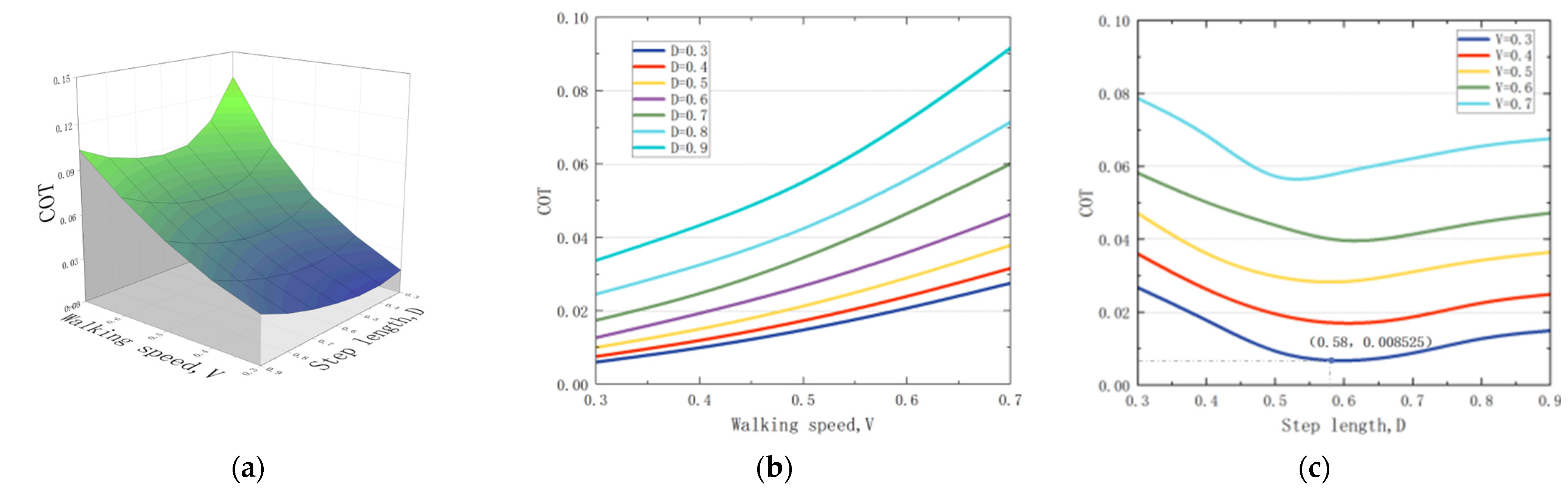
This section describes the validation of the energy optimization method for the bipedal robot, as discussed in the preceding section. A set of fixed mechanism parameters is selected: $l_{bper}=0.2, { l}_{thper}=0.$4, $m_{per}=0.$3, and $m_{hper}=0.$3, and the optimal energy-efficient walking gait for the bipedal robot is determined. The variations in the $COT$ under different walking speeds and step lengths are assessed to clarify their effect.

Figure 3 shows the variations in the robot walking performance at different walking speeds and step lengths. Figure 3b indicates that the $COT$ increases with an increase in the walking speed. Thus, considering a constant walking speed, an optimal step length can be found to minimize $COT$. For instance, in Figure 3c, when V = 0.3 and D = 0.58, the $COT$ attains its minimum value of 0.008525.

4.2. Optimization of Leg Mass Ratio

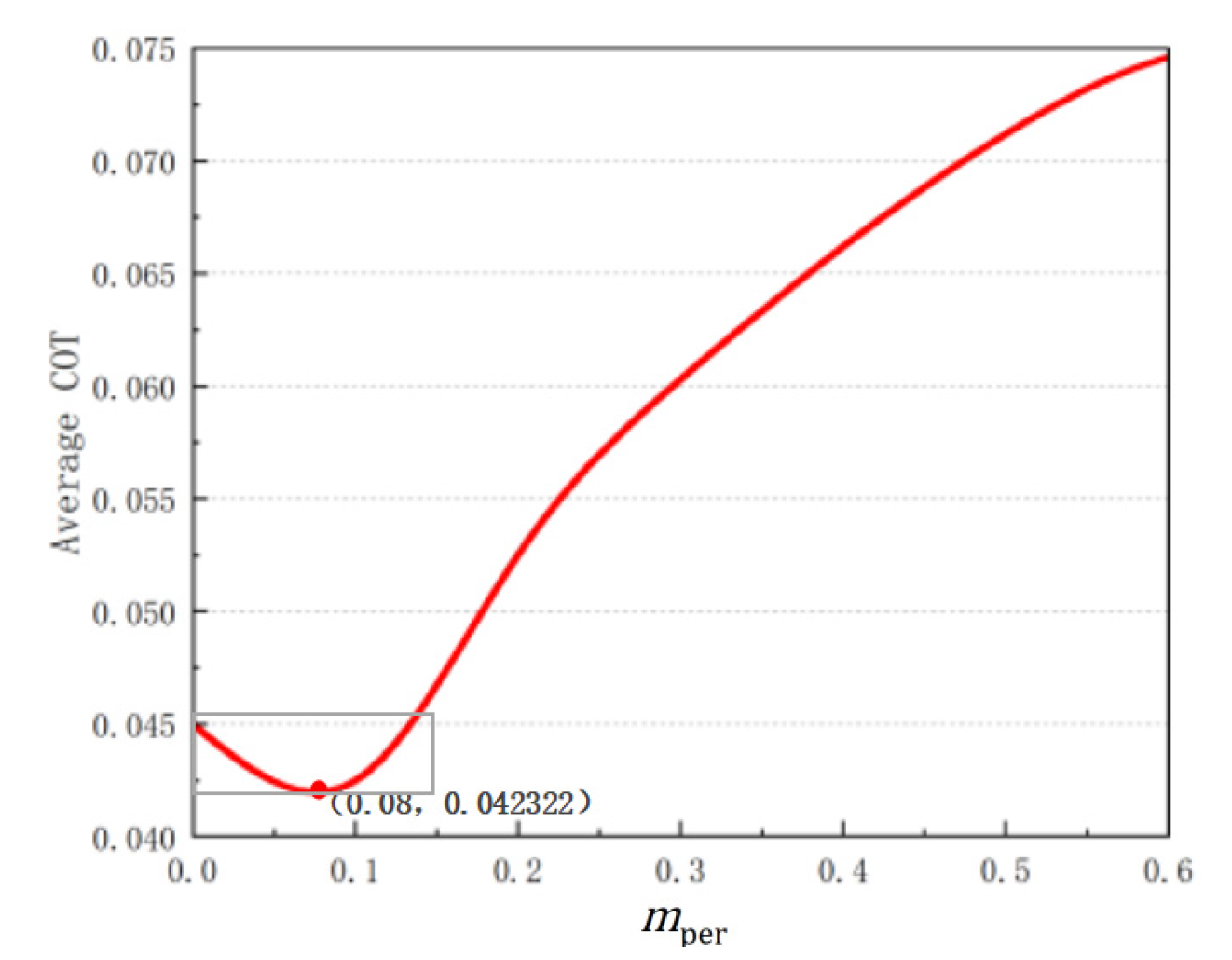
Based on the parameters of the human body structure, the mechanism parameters of the bipedal robot are configured as ${ l}_{bper}=0.2 \mathrm{a}\mathrm{n}\mathrm{d} l_{thper}=0.$4 as the ratio of the robot rod length, the optimal mass ratio of leg to body and hip, $m_{per}$, is analyzed.

Figure 4 shows the variation in the full-range energy consumption ${COT}_{ave}$ when $m_{per}$ varies in the range of [0, 0.6]. The ${COT}_{ave}$ first decreases and then increases with an increase in $m_{per}$. The minimum value, ${COT}_{min}$ of 0.042322, is observed at $m_{per}$ = 0.08. When $m_{per}$ varies in the range of [0, 0.15], ${COT}_{ave}$ consistently remains at a low level.

When the leg mass of the robot constitutes a small proportion of the total body mass, achieving optimal full-range energy consumption becomes more feasible.

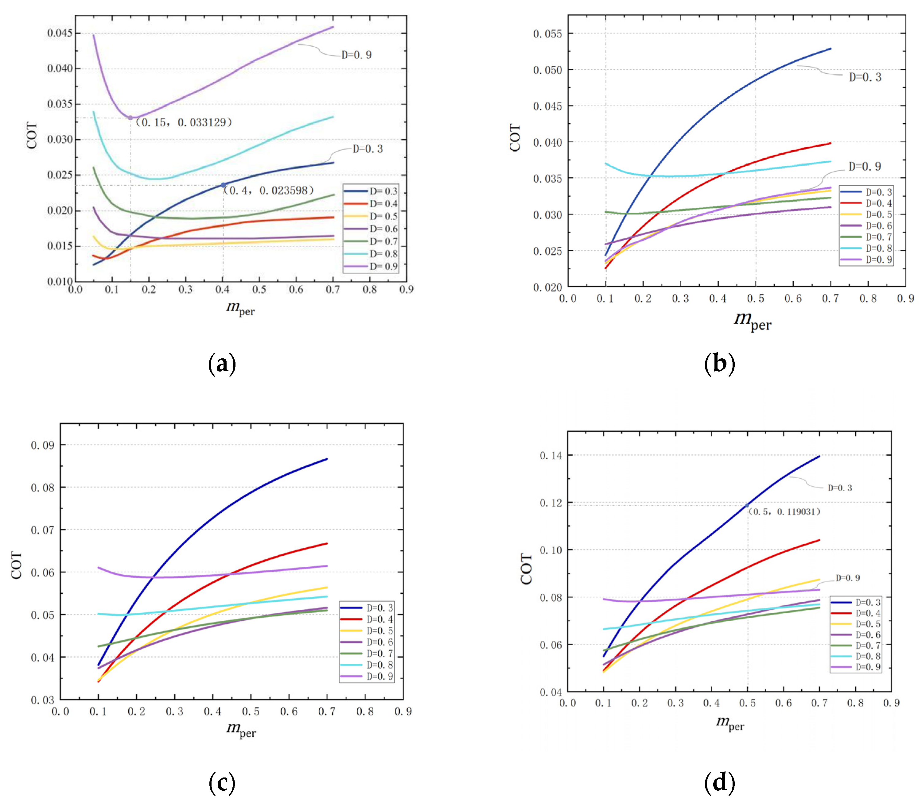
Figure 5 shows that when V = {0.3, 0.4, 0.5, 0.6}, the $COT$ corresponding to the different step lengths changes with $m_{per}$. For large values, i.e., V = {0.4, 0.5, 0.6}, the $COT$ increases with an increase in $m_{per}$ when the step length is short. For example, as shown in Figure 5d, when V = 0.6 and D = 0.3, $COT$ is 0.119031 for $m_{per}$ = 0.5. At longer step length, $m_{per}$ does not considerably affect the $COT$. For example, in Figure 5d, when V = 0.6 and D = 0.9, the $COT$ remains nearly unchanged.

For small values, i.e., V = 0.3, the $COT$ increases with an increase in $m_{per}$ when the step length is short. For example, as shown in Figure 5a, when V = 0.3 and D = 0.3, $COT$ is 0.023598 for $m_{per}$ = 0.4. At longer step lengths, the $COT$ first decreases and then increases with an increase in $m_{per}$. For example, in Figure 5a, when V = 0.3 and D = 0.9, $COT$ is 0.033129 for $m_{per}$ = 0.15.

When $m_{per}$ is small, such as $m_{per}$ = 0.1 in Figure 5b, the $COT$ is small when the step length is short (D = 0.3) and increases with a long step length, i.e., D = 0.9. With an increase in $m_{per}$, $COT$ significantly increases for shorter step lengths. However, the energy consumption of long step length walking remains nearly unchanged with an increase in $m_{per}$.

Figure 5a shows that a smaller $m_{per}$ does not always correspond to a lower full-range energy consumption. For example, as shown in Figure 4, the optimal full-range energy consumption, the minimal $COT$, appears at $m_{per}$ = 0.08.

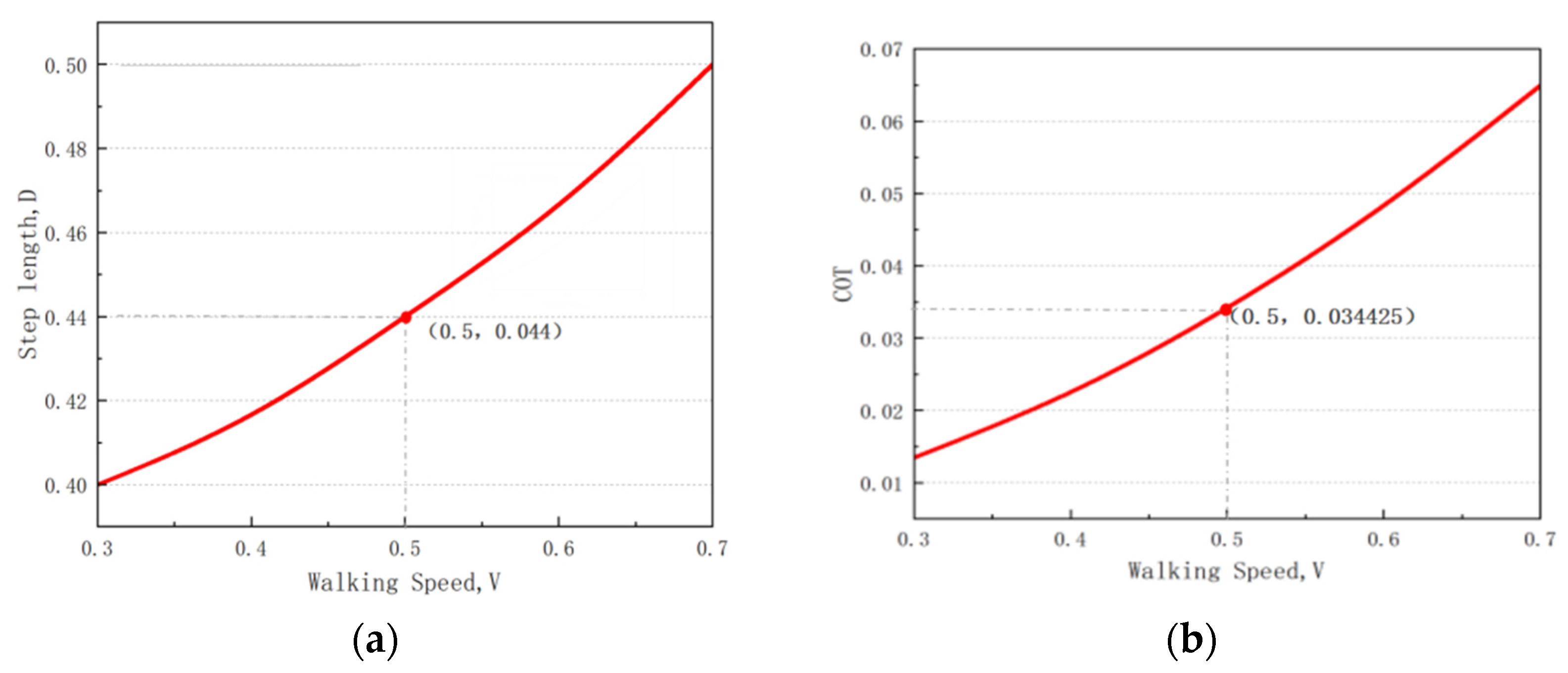
Figure 6 shows the variation in the optimal step length with the walking speed when $m_{per}$ = 0.08 and the $COT$ values correspond to the optimal step length. The optimal step length increases with an increase in the walking speed. For example, in Figure 6, when V = 0.5, the optimal step length D = 0.44, and the corresponding $COT$ is 0.034425.

4.3. Optimization of Hip Mass Ratio

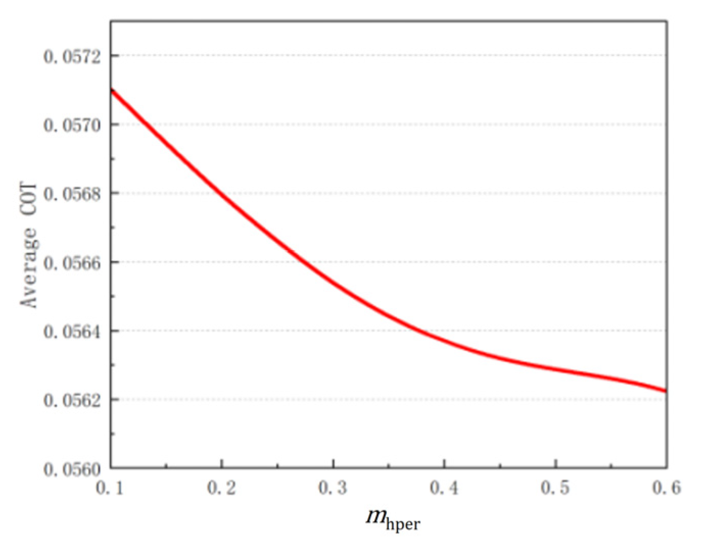
After obtaining the optimal value for the leg mass ratio ${ m}_{per}$, in this section, we refer to the parameters of the human body structure and take $m_{per}=$ 0.3 as the fixed mechanism parameters of the bipedal robot. Keeping the ratio of the robot rod length $l_{bper}=0.2$ and $l_{thper}=0.$4 unchanged, the optimal mass ratio of hip to body, $m_{hper}$, is analyzed.

Figure 7 shows the variation in the full-range energy consumption ${COT}_{ave}$ when $m_{hper}$ varies in the range of [0, 0.6]. The ${COT}_{ave}$ decreases with an increase in $m_{hper}$. When the proportion of the robot’s hip mass to the body mass is large, the bipedal robot’s mechanism exhibits superior performance in terms of full-range energy consumption under the given objective.

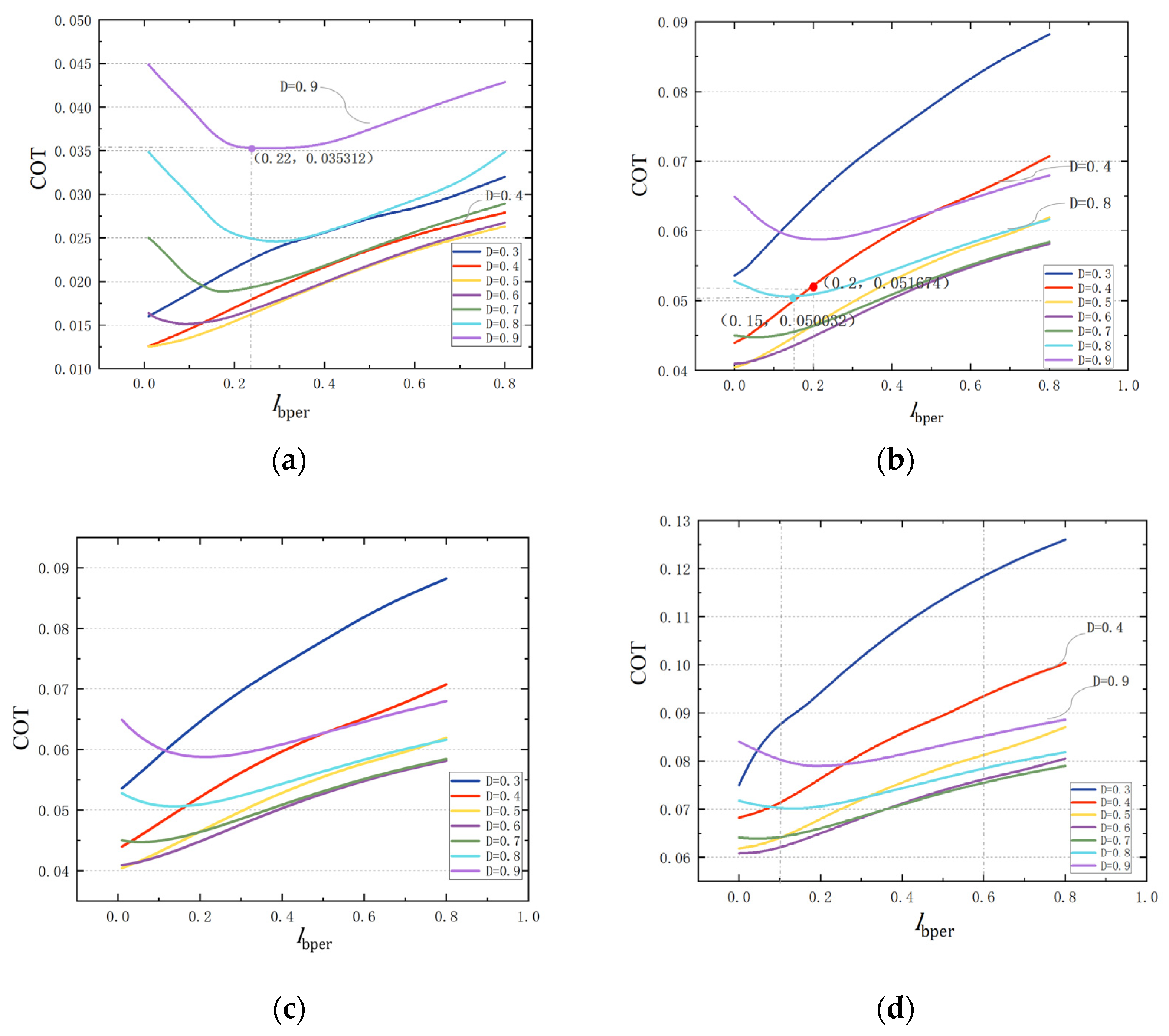
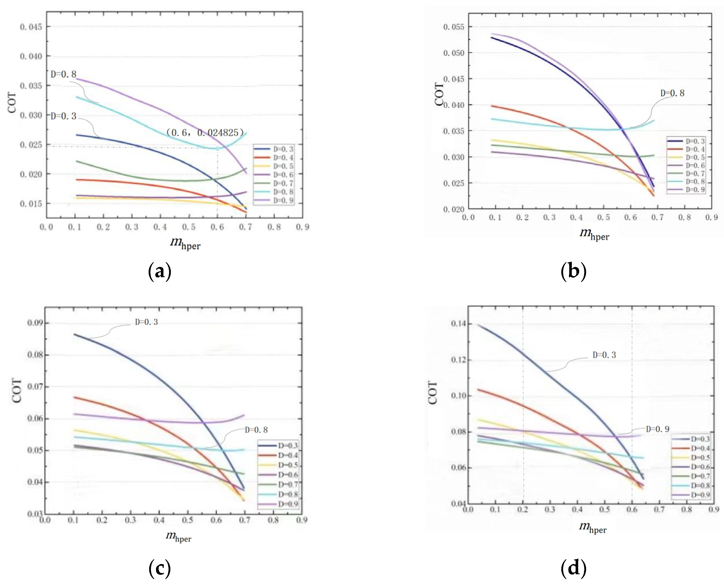
Figure 8 shows that when V = {0.3, 0.4, 0.5, 0.6}, the $COT$ corresponding to the different step lengths changes with $m_{hper}$. The $COT$ decreases with an increase in $m_{hper}$ at different walking speeds when the step length is short. For long step lengths, when the walking speed is large, such as V = 0.6 and D = 0.9 as shown in Figure 8d, $m_{hper}$ does not considerably affect the $COT$. At small walking speeds, the $COT$ first decreases and then increases with an increase in $m_{hper}$, when V = 0.3 and D = 0.8 as shown in Figure 8a; ${COT}_{min}$ is 0.024825 for $m_{hper}$ = 0.6.

When the $m_{hper}$ is small, such as $m_{hper}$ = 0.2 as shown in Figure 8d, the $COT$ is large when the step length is short (D = 0.3) and small at the long step length, i.e., D = 0.9. With an increase in $m_{hper}$, the full-range energy consumption significantly decreases for shorter step lengths. However, the energy consumption of long step length walking remains nearly unchanged with aan increase in $m_{hper}$.

As shown in Figure 8, the value of longer step length remains relatively stable as $m_{hper}$ changes. When $m_{hper}$ is larger, the value of $COT$ for shorter step length is relatively smaller. Therefore, for larger $m_{hper}$, the designed walking gait achieves optimal full-range energy consumption.

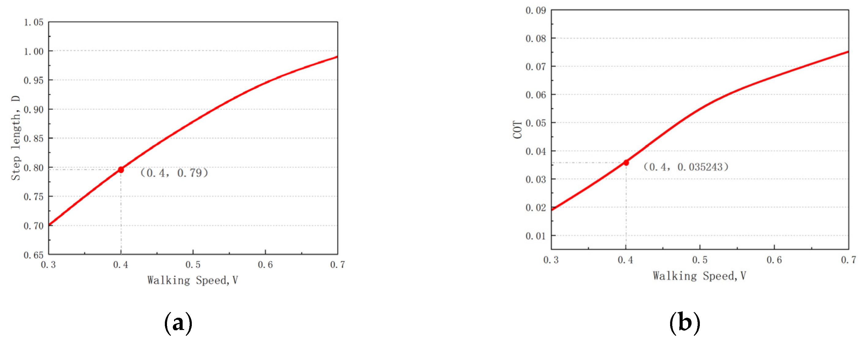
Figure 9 shows the variation in the optimal step length with the walking speed when $m_{hper}$ = 0.3 and the $COT$ values correspond to the optimal step length. The optimal step length increases with na increase in walking speed.

4.4. Optimization of Leg Length Ratio

After obtaining the optimal value for the leg mass ratio ${ m}_{per}$ and hip mass ratio $m_{hper}$, the mechanism parameters of the bipedal robot are set as $l_{bper}=0.2$, $m_{per}=0.$3, and $m_{hper}=0.$3, and the length ratio of body to leg, $l_{thper}$, is analyzed.

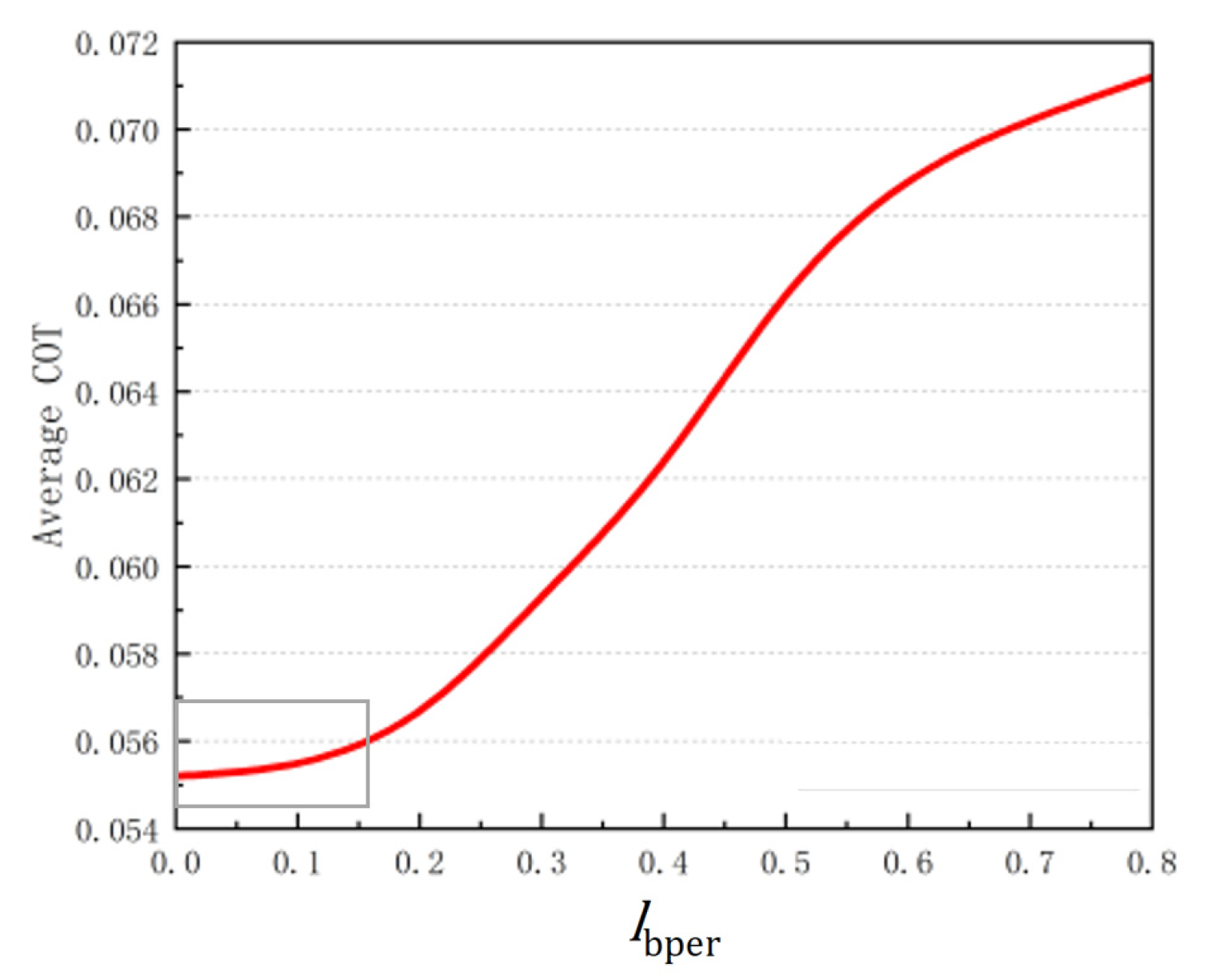
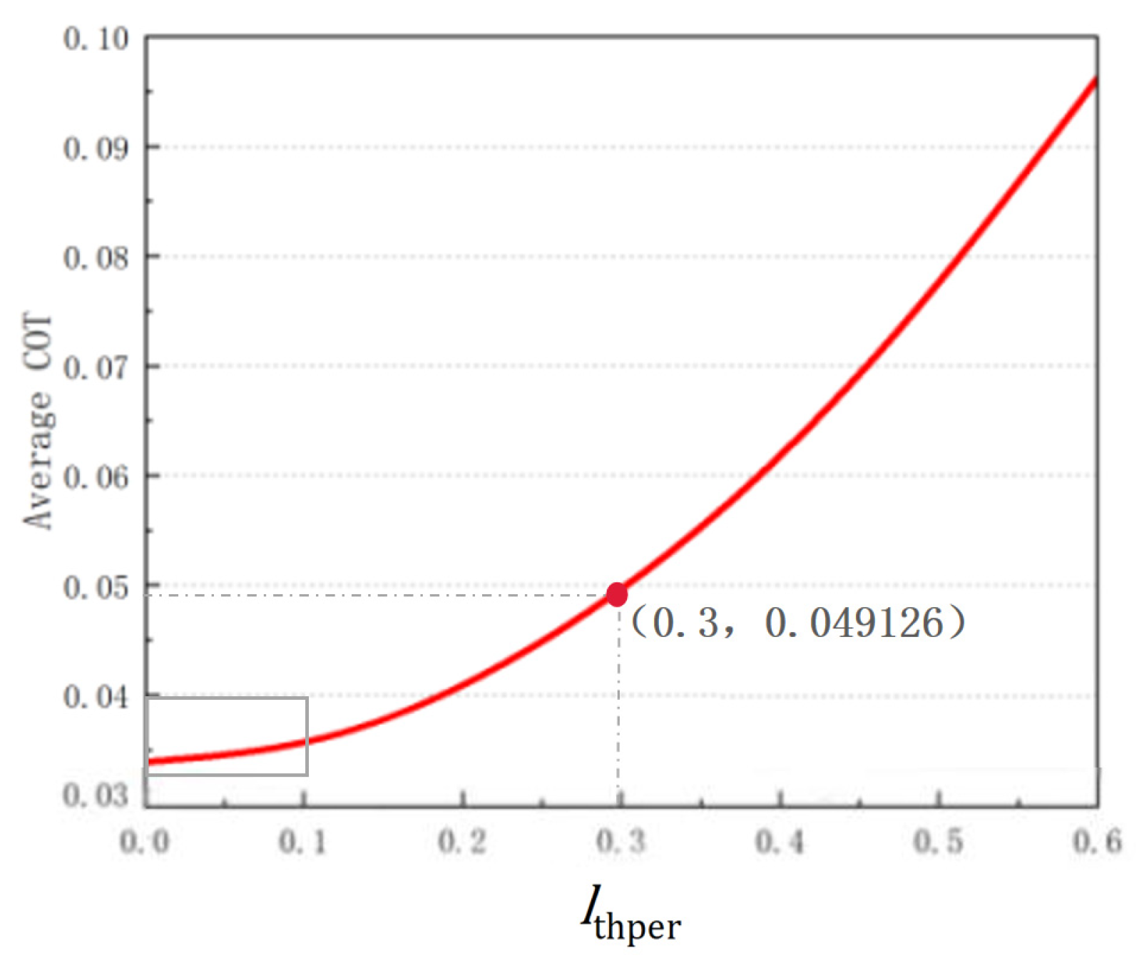
Figure 10 shows the variation in the full-range energy consumption ${COT}_{ave}$ when $l_{thper}$ varies in the range of [0, 0.6]. The ${COT}_{ave}$ increases with an increase in $l_{thper}$. ${COT}_{ave}$ of 0.049126 is observed at $l_{thper}$ = 0.3. When $l_{thper}$ varies in the range [0, 0.1], ${COT}_{ave}$ consistently remains at a low level. It can be observed that the bipedal robot exhibits higher average efficiency in walking when the distance between the center of mass of the hip and the leg is closer.

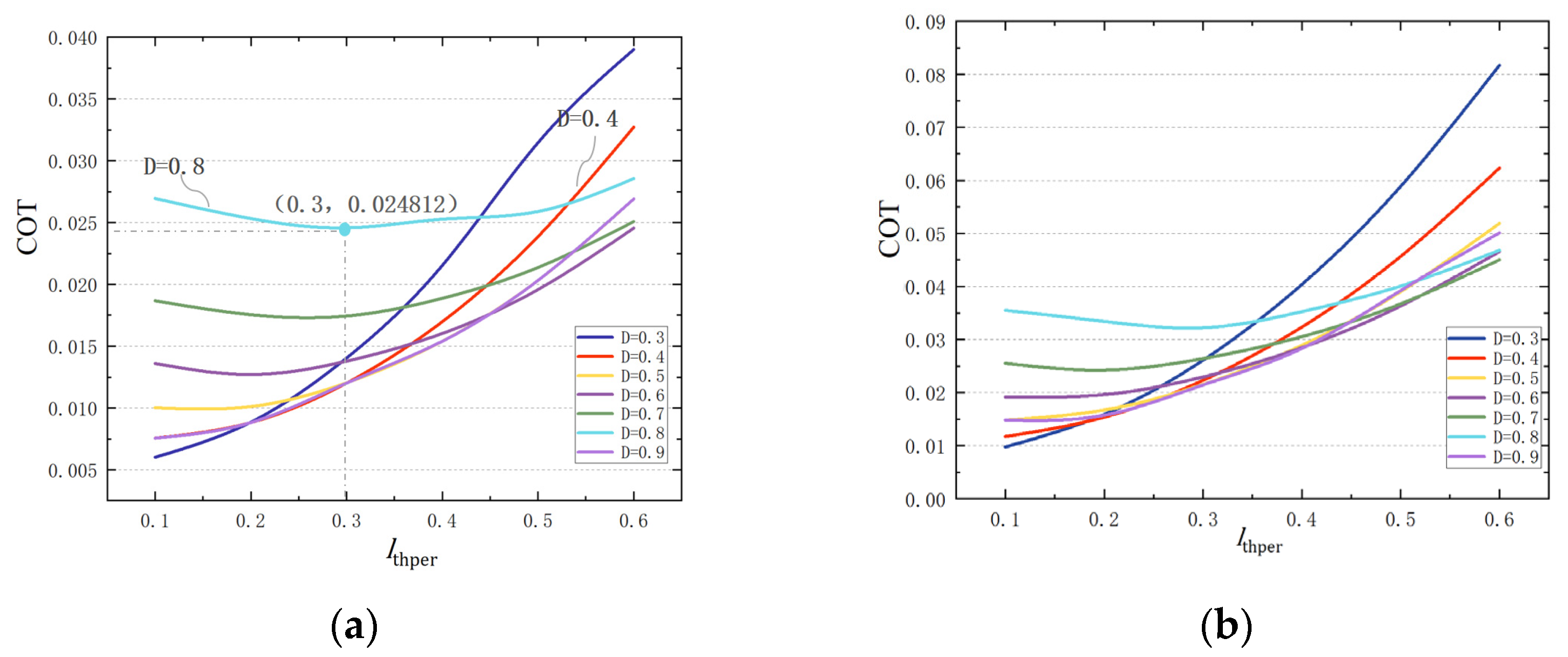
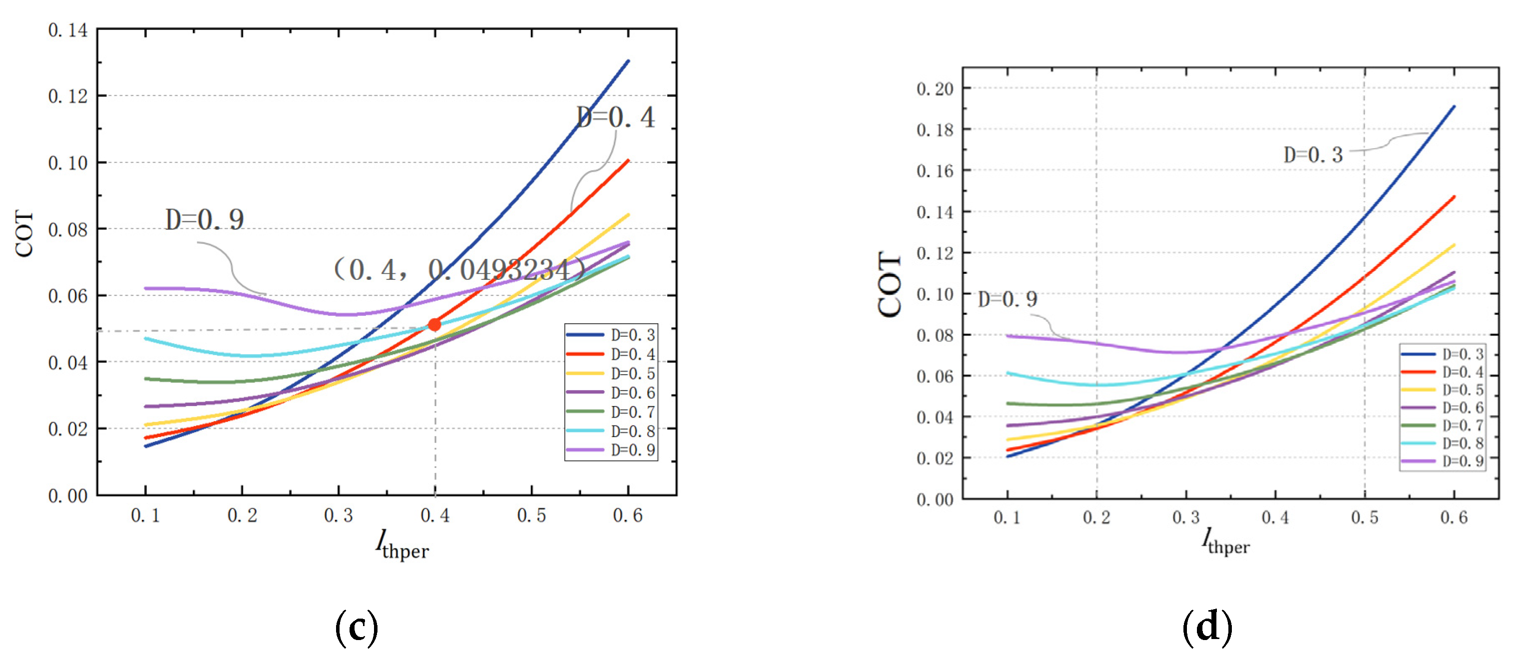
As shown in Figure 11, the energy consumption $COT$ corresponding to different step lengths is depicted for the range of V = {0.3, 0.4, 0.5, 0.6}, with respect to the variation in $l_{thper}$. The $COT$ increases with an increase in $l_{thper}$ when the walking speed remains constant and the step length is short (Figure 11c: V = 0.5 and D = 0.4). At longer step lengths, the ${COT}_{ave}$ first decreases and then increases with an increase in $l_{thper}$, and the overall trend changes steadily. In Figure 11a, when V = 0.3 and D = 0.8, the minimum energy consumption value $COT$ is 0.024812 for $l_{thper}$= 0.3.

By comparing the variation in $COT$ with different step lengths, it can be observed that when ${ l}_{thper}$ is smaller, the $COT$ value is lower. This means that selecting a smaller value of ${ l}_{thper}$ results in the optimized configuration having higher ground adaptability.

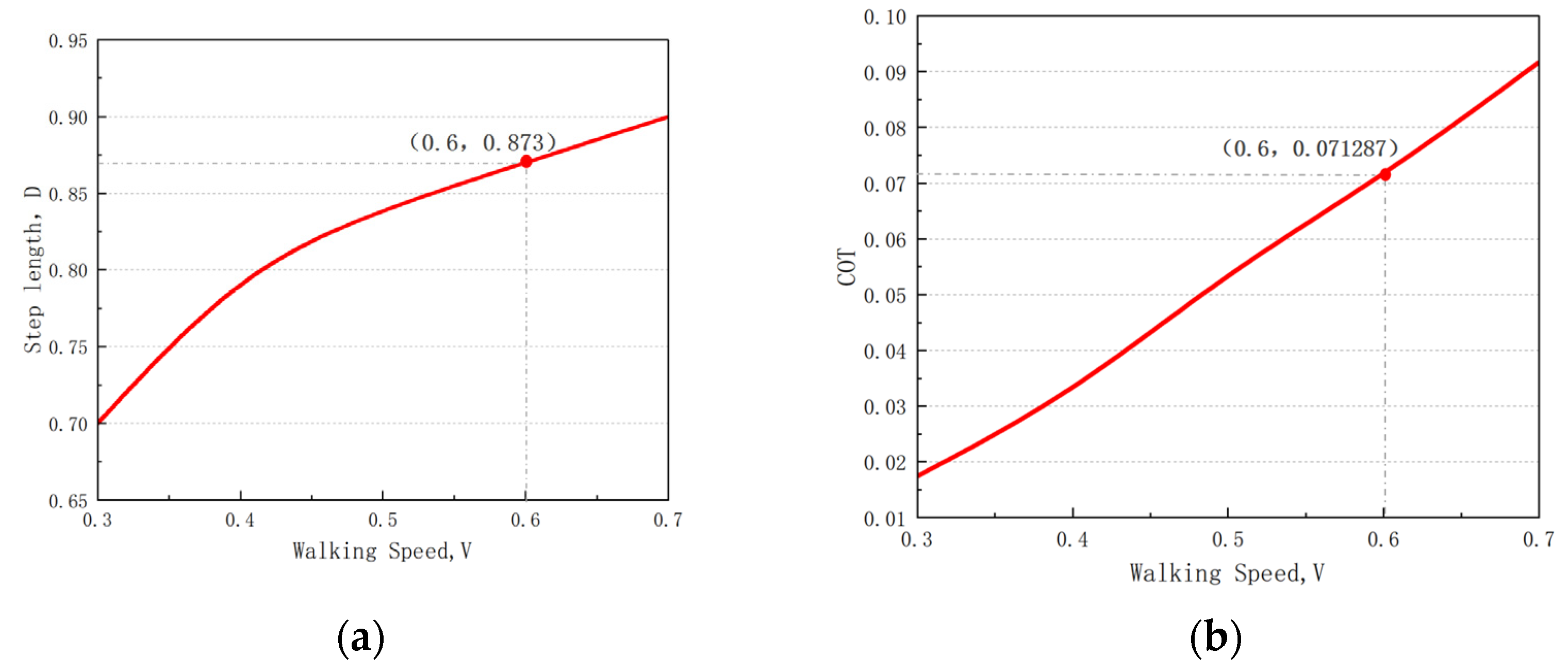
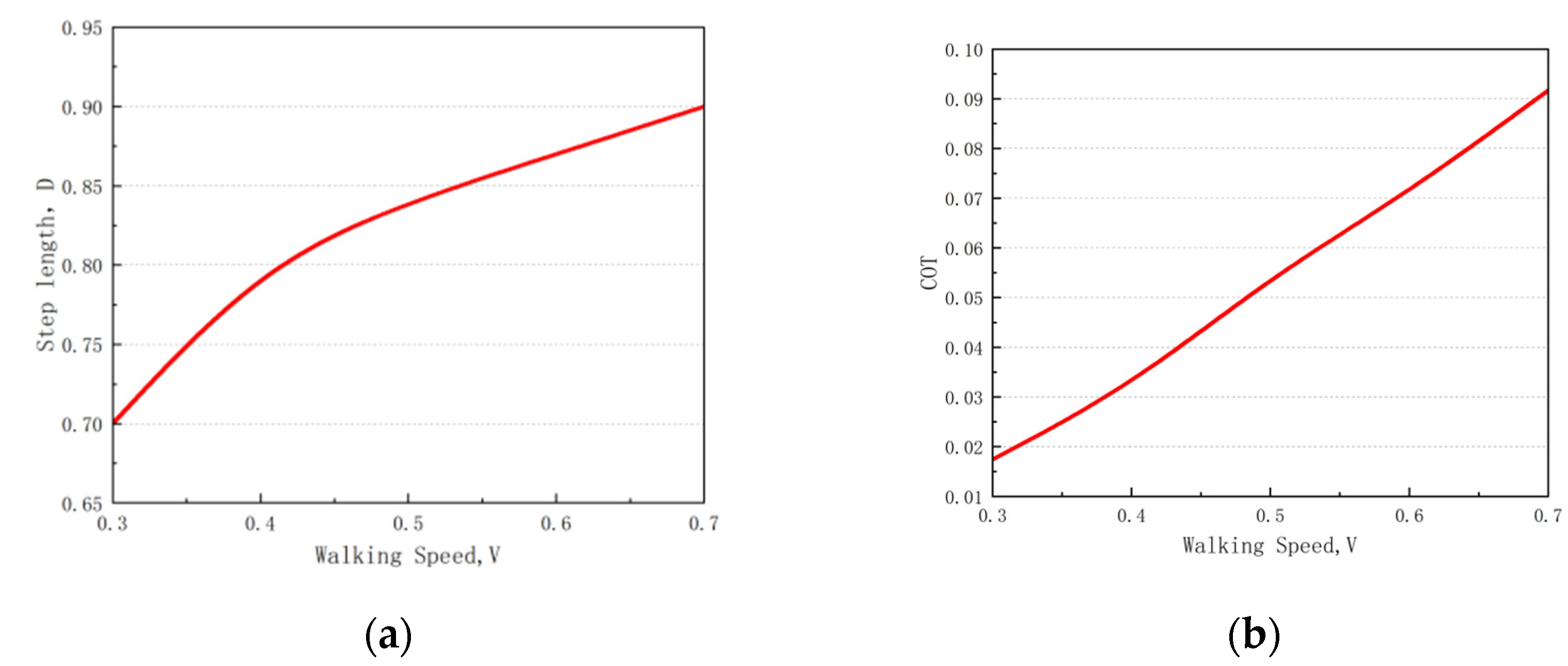
As shown in Figure 12, the variation in the optimal step length and the corresponding optimal $COT$ are depicted when $l_{thper}$ is fixed at 0.3. At different walking speeds, it is possible to find the corresponding step length that minimizes the $COT$ (V = 0.6, D = 0.873, and $COT$ = 0.071287).

4.5. Optimization of Upper Body Length Ratio

After obtaining the optimal value for $l_{thper}$, $m_{per}$, and $m_{hper}$, the mechanism parameters of the bipedal robot are set as $l_{thper}=0.$4, $m_{per}=0.$3, and $m_{hper}=0.$3, and the optimal position of the center of the length of the upper body,${ l}_{bper}$, is analyzed.

Figure 13 shows the variation in the full-range energy consumption ${COT}_{ave}$ when $l_{bper}$ varies in the range of [0, 0.8]. The ${COT}_{ave}$ increases with an increase in $l_{bper}$. Moreover, when $l_{bper}$ varies in the range of [0, 0.15], and ${COT}_{ave}$ remains relatively stable. It can be observed that as the ratio of the robot’s upper body to total body length increases, the optimized configuration tends to have higher energy efficiency.

Figure 14 shows that when V = {0.3, 0.4, 0.5, 0.6}, the $COT$ corresponding to the different step lengths changes with $l_{bper}$. When the walking speed is fixed and the step length is short, the energy consumption $COT$ increases with an increase in $l_{bper}$. At long step length, the energy consumption $COT$ first decreases and then increases with an increase in $l_{bper}$ (Figure 14b: V = 0.4 and D = 0.4, 0.8).

With an increase in $l_{bper}$, the walking energy consumption significantly increases for a shorter step length; it first decreases and then increases when the step length is long. Therefore, with a decreasing value of $l_{bper}$, the optimized configuration exhibits a more stable walking gait.

Figure 15 shows the variation in the optimal step length with the walking speed when $l_{bper}$ = 0.4 and the $COT$ values correspond to the optimal step length. The optimal step length increases with an increase in walking speed.

The above research results show that reducing the ratio of leg mass in the total mass, concentrating the mass of the entire body at the hip joint, reducing the ratio of the upper body to total body length, and increasing the height of the leg center of mass can enhance the performance of the optimized mechanism.

4.6. Optimization of Gait

Under different mechanism parameters, i.e., $m_{per}, m_{hper}, l_{bper}, \mathrm{a}\mathrm{n}\mathrm{d} l_{thper}$, bipedal robots walking at various walking speeds and step lengths have varying energy consumption requirements. 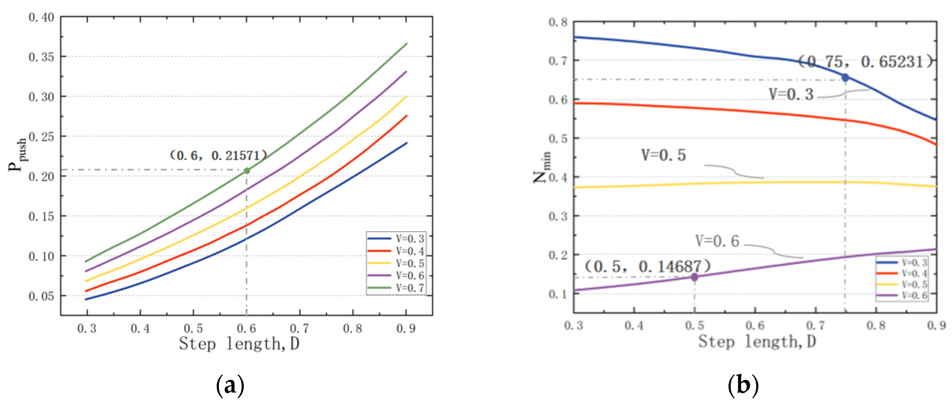Based on the human body structure parameters and practical aspects of robot design, this section focuses on studying the walking gait features of bipedal robots based on the analysis above; the bipedal robots are set as $m_{per}=0.$3, $m_{hper}=0.$3, $l_{bper}=0.15$, and $l_{thper}=0.$ The push-off impulse $P_{push}$ and minimum ground reaction force $N_{min}$ under different step lengths and walking speeds are determined. The minimum ground support force refers to the minimum vertical support force exerted by the ground on the bipedal robot throughout the swing phase. When the support force is less than zero, the robot’s legs are off the ground. Figure 16a shows that the $P_{push}$ increases with an increase in walking speed and step length.

As shown in Figure 16b, throughout the swing phase, for small walking speeds, the $N_{min}$ decreases with an increase in step length. The $N_{min}$ increases with an increase in step length when the walking speed is large. It is also observed that for moderate walking speed, the $N_{min}$ remains relatively constant (Figure 17b, V = 0.3, 0.5, and 0.6).

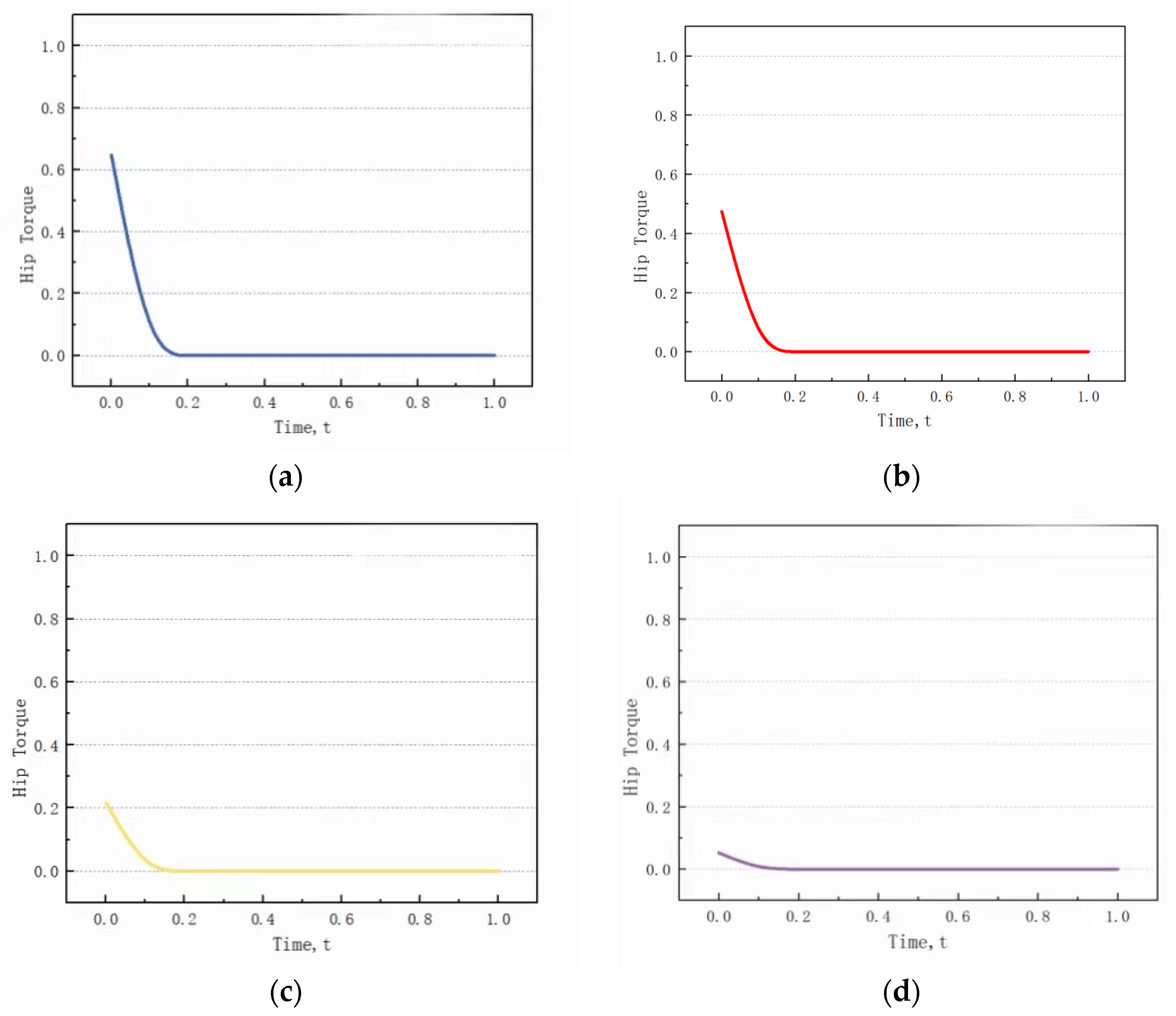
According to optimal mechanism parameters, Figure 17 shows the variation in hip joint torque ${\tau }_{hip}$ corresponding to different step lengths under the condition of fixed walking speed. The hip joint torque exhibits positive values only during the initial phase of the swing phase. And thereafter, it remains at zero throughout the walking motion. Under the same walking speed, the hip joint torque ${\tau }_{hip}$ required for cyclic walking gait decreases with an increase in step length. The ankle joint torque has no effect during motion on flat ground and remains at 0.

In this model, the hip joint torque serves as the primary driving force during the swing phase, and it only exists at the beginning of the gait. On the other hand, in the push-off phase, ankle joint torque is the sole driving force in this model, and it only exists when the gait is about to end. Figure 18 shows that when walking with a short step length, a smaller push-off impulse is adequate to successfully complete the swing of the stance leg. The duration of the swing phase is relatively short, so the swing leg needs to generate a larger torque by the hip to complete the swing quickly. As the step length increases, a larger push-off impulse is necessary to enable the swing of the stance leg during the swing phase. At this point, the duration of the swing phase increases, and the swing leg only needs a smaller torque to complete the swing. At the same walking speed, for longer step lengths, the required hip joint torque is smaller, and the push-off impulse is larger during the swing phase. By comparing with the former study, the above common features can be identified [36,37].

Therefore, based on the analysis in this paper, the following design recommendations can be derived. In designing the walking gait of a bipedal robot, the swing phase should provide a forward hip joint torque to drive the swing of the swing leg, and at the moment the swing leg leaves the ground, a push-off impulse is provided to complete the ankle joint to push off. These coordinated actions are performed to accomplish the entire walking motion, leading to the subsequent transition to the next step of the cycle.

5. Conclusions

This paper established a dynamic parameter optimization model for bipedal robots based on full-range walking energy efficiency to solve the optimal walking gait subject to the walking constraints.

Investigating the optimal linkage mechanism for bipedal robots and analyzing the influence of the robot’s dynamic parameters on walking energy efficiency indicate that reducing the ratio of leg mass in the total mass, concentrating the mass of the entire body at the hip joint, reducing the ratio of the upper body to total body length, and increasing the height of the leg center of the mass can enhance the performance of the optimized mechanism and result in higher energy efficiency. By calculating the ground contact impulse, minimum ground support force, and torque characteristics of the walking gait at a fixed speed, we found that during the swing phase of the walking gait, initial forward hip joint torque is responsible for initiating the forward movement of the swing leg while the torque remains at zero during the subsequent phase. Under fixed speed conditions, as the step length increases, the torque required to drive the swing leg decreases gradually while the impulse for ground push-off increases, ensuring the stability and low energy consumption of bipedal robot walking. These actions are coordinated to complete the whole walking motion. For smaller step lengths, the optimal walking gait involves larger swing torque and smaller push-off impulse, whereas it is the opposite for the longer step length.

The research findings of this paper not only contribute to a deeper understanding of efficient walking mechanisms but also provide important references for the design of mechanisms and walking gait for bipedal robots.