Contrast Enhancement-Based Preprocessing Process to Improve Deep Learning Object Task Performance and Results

Abstract

Excessive lighting or sunlight can make it difficult to judge visually. The same goes for cameras that function like the human eye. In the field of computer vision, object tasks have a significant impact on performance depending on how much object information is provided. Light presents difficulties in recognizing objects, and recognition is not easy in shadows or dark areas. In this paper, we propose a contrast enhancement-based preprocessing process to obtain improved results in object recognition tasks by solving problems that occur due to light or lighting conditions. The proposed preprocessing process involves the steps of extracting optimal values, generating optimal images, and evaluating quality and similarity, and it can be applied to the generation of training and input data. As a result of an experiment in which the preprocessing process was applied to an object task, the object task results for areas with shadows or low contrast were improved while the existing performance was maintained for datasets that require contrast enhancement technology.

1. Introduction

Light is one of the biggest factors that make it difficult to recognize the original shape of an object by lowering the object recognition rate. If the lighting conditions are bright or rough, the object may be blurred or overexposed, making it difficult to distinguish the object’s features [1,2,3]. Additionally, shadows caused by increased contrast from light may obscure important information about an object’s shape and size [4,5]. Figure 1 is an example image showing problems caused by indoor and outdoor light. In the case of the chairs and apples, there are shadows or low-light areas on the objects depending on the location of sunlight or lighting, and in the case of the grapes, there are partially overexposed areas. Such phenomena inevitably occur where there is a luminous object, and this can make it difficult to guess or detect the exact size or number of objects, so methods or algorithms for improvement are needed. Additionally, these phenomena degrade image data quality, with the quality deteriorating more significantly outdoors than indoors. In particular, image contrast can have a significant impact on the performance of object recognition algorithms because it is determined by the amount of light [6].

One of the most important tasks in computer vision is object recognition, a task that identifies and classifies objects within images (videos) [7]. Deep learning-based object recognition algorithms, such as convolutional neural networks (CNNs), have achieved state-of-the-art performance in object recognition tasks, and, more recently, models such as Vision Transformer (ViT) are also achieving state-of-the-art (SOTA) performance [8,9]. These deep learning-based object recognition algorithms are highly dependent on the environmental factors which affect the quality of the training data, so model performance may deteriorate due to insufficient training data, large amounts of noise, and the presence of unlearned environmental factors [10,11]. Therefore, it is important to make the environmental factors and quality of training data and input data the same [12].

In addition, it is difficult to completely solve problems caused by lighting conditions, even with deep learning-based object recognition algorithms. Therefore, in object recognition tasks (classification, detection, segmentation), the preprocessing of training or input image data is necessary to improve recognition results for problem areas that appear according to the performance of the learning model and lighting conditions. In addition, deep learning technology that uses a lot of computing resources has emerged due to the development of big data and hardware devices such as CPUs, GPUs, and TPUs. However, image data improvement technology that uses deep learning algorithms has the following disadvantages: (1) overfitting problems due to lack of training data; (2) generalization performance degradation problems due to biases in training data; and (3) speed reduction problems due to high amounts of computation and memory usage [13,14]. In particular, problems such as slowdown occur in unmanned vehicles, which require a small amount of computing resources [15].

Therefore, in order to obtain improved results in the object recognition task by solving the problems caused by light or lighting conditions, this paper proposes a contrast enhancement-based preprocessing process. The proposed preprocessing process involves a method to improve images using statistical techniques which was devised to reduce the computational process. The proposed process suggests a way in which a similar environment can be built by improving the learning data and the input data; greater similarity between the learning data and the input data environment of the object recognition process will enable more accurate results to be obtained.

2. Related Works

In the process of researching this thesis, problems caused by light or lighting were confirmed, as was the progress achieved in previous and related studies, and the research was conducted based on the contents of the contrast enhancement technique, which is a basic technology that can be improved.

2.1. Problems Caused by Light

The problematic phenomena exhibited by light have a significant impact on object recognition in computer vision systems. Different lighting conditions affect the way objects appear and their visual characteristics, making recognition difficult. These include shadows, fade, overexposure, missing information, reflections, occlusion, color temperature shifts, and noise. To overcome these challenges, computer vision algorithms use techniques such as image normalization, light constancy, and shadow detection to improve object recognition robustness under different lighting conditions. These strategies help improve the accuracy and reliability of computer vision systems that recognize objects in different lighting conditions. Accordingly, various studies are being conducted to improve problems caused by light [16,17,18].

2.2. Contrast Enhancement Method

The contrast enhancement method refers to a method of improving image quality or facilitating image recognition by clarifying the differences between the dark and bright areas of an image. There are several types of contrast enhancement methods:

2.2.1. Color Space Conversion

In the case of color images, this method applies contrast adjustment only to the luminance channel by converting from the RGB color space to a color space with a luminance component (e.g., HSV). This method can maintain the original color while enhancing the contrast of color images [19].

2.2.2. Intensity Value Mapping

This method adjusts the contrast by mapping the contrast value of the input image to a new value. With this method, the user can define the mapping function directly, and functions such as imadjust, histeq, and adapthisteq can be used [20].

2.2.3. Local Contrast Enhancement

This is a method of dividing an image into small regions and applying histogram equalization for each region. Although this method can improve detailed contrast more than the global method, it has problems such as blocking or loss of harmony [21].

2.2.4. Histogram Equalization (HE)

This is a method to increase the contrast by making the histogram of the image uniform. Although this method is simple and effective, it can cause color distortion or noise due to changes in the average brightness of the image or excessive contrast increases [22].

2.2.5. Adaptive Histogram Equalization (AHE)

This is a method of dividing an image into smaller parts and applying histogram equalization to each part. This method can improve local contrast, but it can amplify noise or sharpen the boundaries between parts [23].

Among the various adaptive histogram equalization techniques, CLAHE (contrast limited adaptive histogram equalization) is an image processing method that suppresses noise while enhancing the contrast of an image [24]. The CLAHE technique achieves equalization over the entire image by dividing the image into small blocks of uniform size and performing histogram equalization on a block-by-block basis. When the histogram equalization is completed for each block, the boundary between blocks is smoothed by applying bilinear interpolation. The CLAHE method redistributes pixel values above a certain height by limiting the histogram height before calculation. The transformed image has characteristics similar to those of the actual image because it is converted in such a way that it is robust to noise located in low-contrast areas. CLAHE is simple; processed images can be reverted to their original form with the inverse operator, the properties of the original histogram can be preserved, and it is a good way to adjust the local contrast of an image. However, it increases noise when pixel intensities are clustered in very narrow areas, and this can lead to the enhancement of the pixel intensity of missing parts (noise amplification), and it is important to properly set parameters such as tileGridSize and clipLimit [25].

Each of the above contrast enhancement techniques has advantages and disadvantages, so the selection of an appropriate technique or the use of a combination of techniques is recommended. Recently, research and efforts to improve video images using deep learning technology have been actively conducted [26,27].

2.3. Image Quality Assessment (IQA)

IQA is a field of computer vision research that focuses on evaluating image quality by evaluating the degree of loss or degradation caused by various distortions such as blurring, white noise, and compression. This task involves analyzing a given image and determining whether it is of good or bad quality. The IQA algorithm quantifies the perceived visual fidelity of an image by taking a random image as input and producing a quality score as output [28,29]. There are three types of IQA: full-reference (FR), reduced-reference (RR), and no-reference (NR) [30]. FR-IQA requires clean original images to evaluate image quality and compares the distorted image to the original to provide a quality score. RR-IQA requires some information from the original image and evaluates image quality based on features extracted from both the distorted image and the reference image. NR-IQA does not require any reference to the original image; it evaluates image quality using manually extracted features from distorted images. NR-IQA methods require training, are label-dependent, and are difficult to apply due to the subjective nature of image quality perception. As a result, it may not be possible to generalize NR-IQA models trained on unstable labels to diverse datasets. IQA methods include representative PSNR, SSIM, VIF, MAD, FSIM, GSM, GMSD, and BRISQUE. In addition, algorithms which use machine learning or deep learning, such as blind multiple reference images-based measure (BMPRI), DeepFL-IQA, and DISTS, have been proposed due to the continuous development of artificial intelligence technology [31,32,33,34,35,36,37,38].

2.4. Feature Point Detection and Matching

Feature point detection is the process of finding parts that express important information or patterns within an image. This process aims to determine the local variation or structure of an image, helping the computer to identify specific points within the image. A typical procedure for feature point detection consists of five steps: image preparation and preprocessing, scale space setup, feature value calculation, keypoint selection, and duplicate removal and alignment. There are various representative algorithms, such as SIFT, SURF, and ORB [39,40,41]. Recently, algorithms which use deep learning, such as SuperPoint, D2-Net, LF-Net, and R2D2, have been used [42,43,44,45]. Feature point matching is the process of finding a corresponding feature point pair between two images by comparing feature points extracted from different images or videos. There are various representative algorithms, such as nearest neighbor (NN), k-nearest neighbors (KNN), and fast library for approximate nearest neighbors (FLANN) [46,47,48]. Recently, deep learning-based feature point matching algorithms such as SuperGlue, DeepCompare, and GeoDesc have been developed and studied [49,50,51].

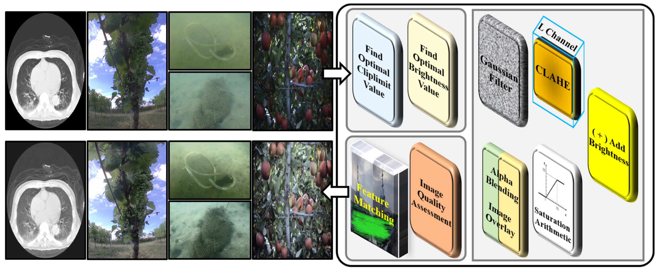
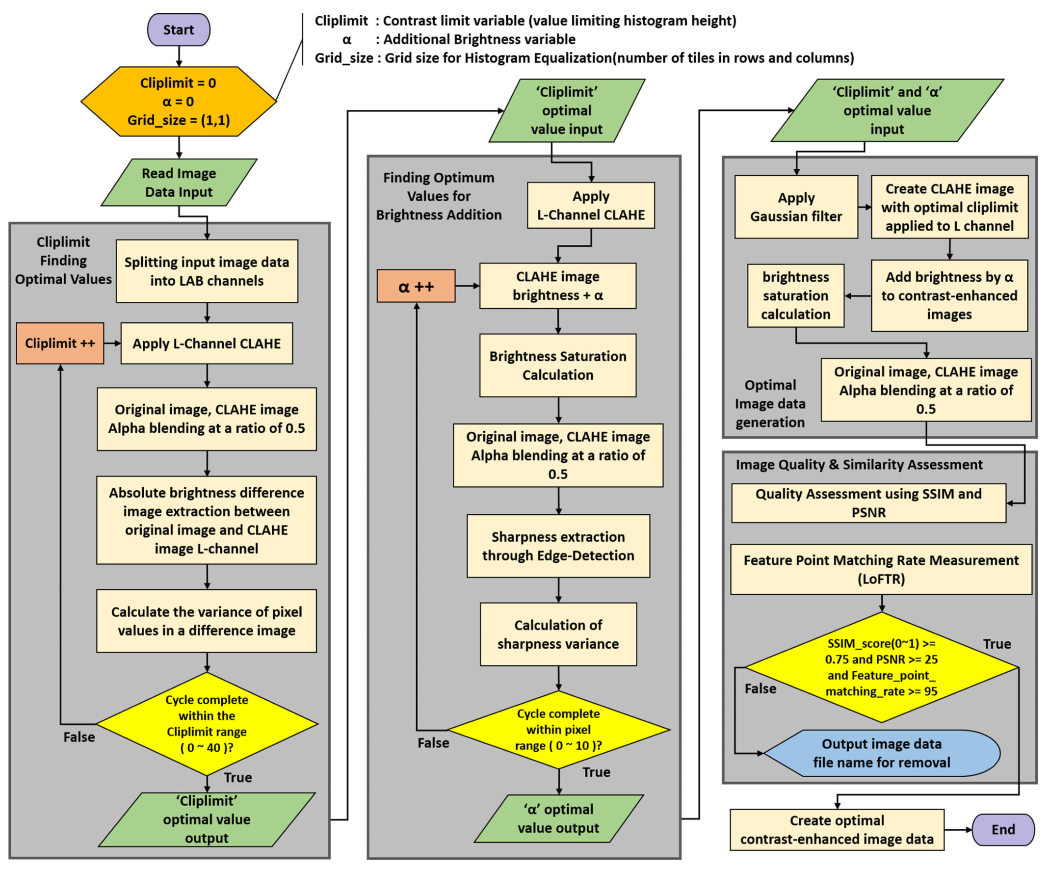
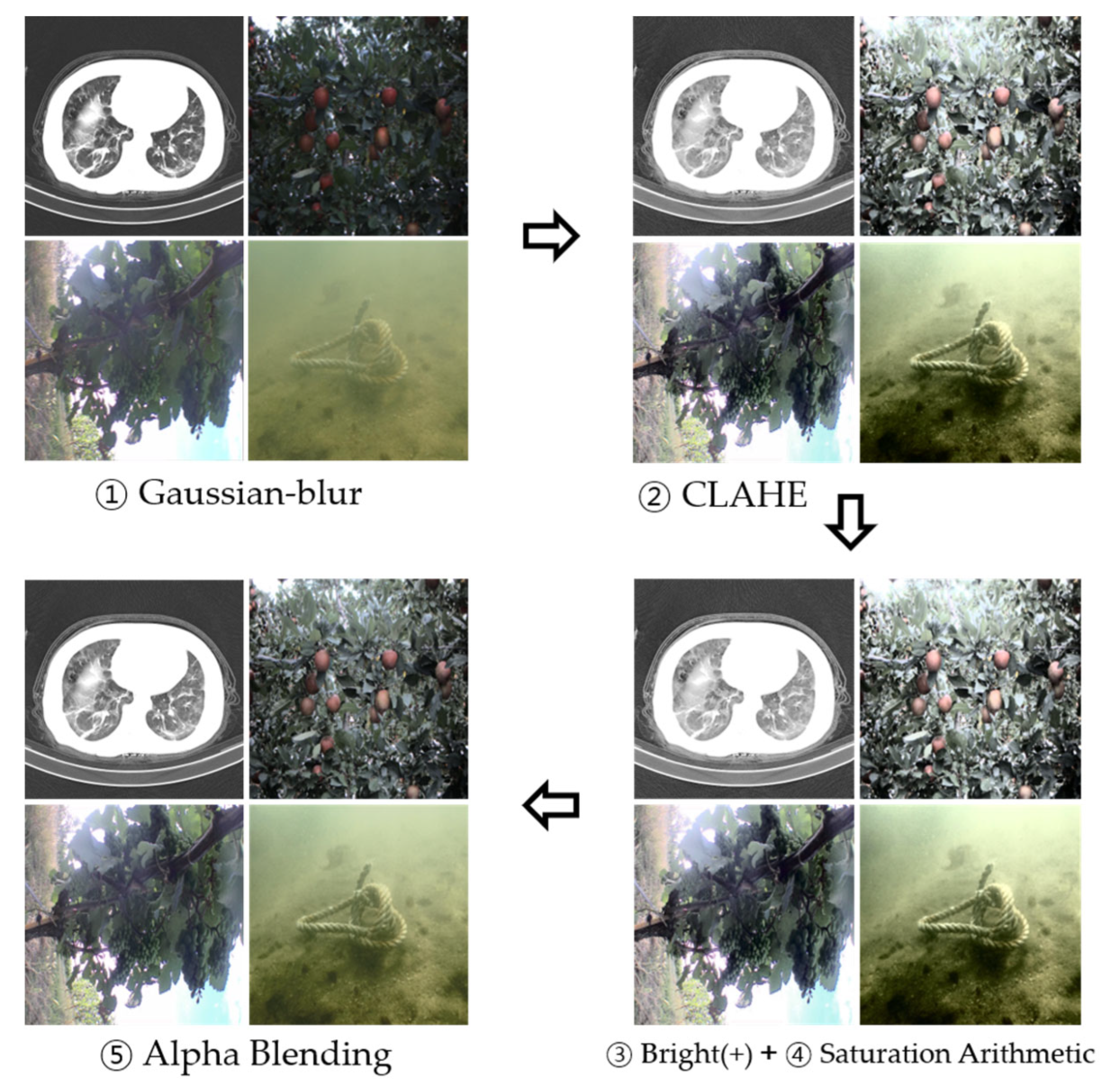
3. Preprocessing Process

The preprocessing process proposed in this paper was created using Python, and Figure 2 and Figure 3 show the preprocessing process diagram and flow chart. When an original image is input through Figure 2 and Figure 3, you can see the process by which the resulting image is created through the stages of ‘Finding optimal values’, ‘Optimal image data generation’, and ‘Quality & Similarity assessment’.

The first and second gray block steps in the flow chart are steps for extracting the optimal values of ‘Cliplimit’ and ‘α (Brightness Addition)’. These steps are responsible for creating contrast-enhanced images and searching for the values needed to improve shadows or low-light areas, respectively. The third gray block step is responsible for creating the optimal image based on the extracted values. The final gray block step is responsible for evaluating how different the generated image is from the original image.

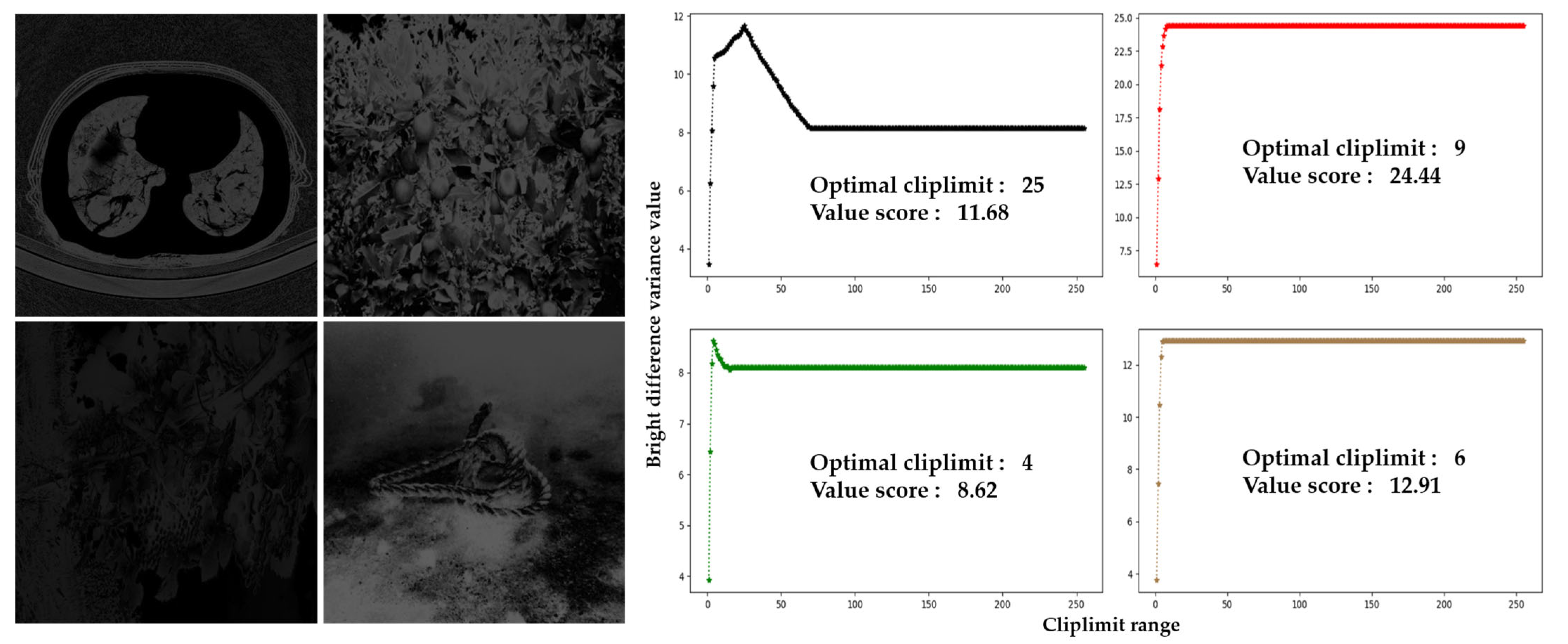
3.1. Finding Optimal Values

Since the illumination or shadow area of an object in image data varies depending on location, time, and environmental factors, it is necessary to find the optimal value when applying contrast enhancement techniques. In this paper, OpenCV’s CLAHE algorithm was applied to the preprocessing process as a contrast enhancement technique.

In the optimal value extraction step, the optimal value for the ‘contrast limit warning value’, called cliplimit, and the ‘additional brightness(α)’ to be applied to improve the shadow area are obtained.

The ‘cliplimit’ optimal value is obtained when the absolute brightness difference between the original image and the simple CLAHE-applied image is calculated. The variance of the pixel values is then calculated in the difference image, and this process is repeated for the cliplimit parameter range (0–255). The maximum variance value is designated as the optimal value.

In the CLAHE algorithm, as the value of the ‘cliplimit’ parameter increases, more aggressive contrast enhancement occurs, and noise and artifacts may be excessively amplified. On the other hand, lower values may not improve contrast enough. The absolute difference in brightness between the two images indicates how much the pixel values have changed after the contrast enhancement. The variance calculation process is a measure of how spread out the pixel values are from the average value, with high variance values indicating a significant range of pixel values and low variance values indicating that the pixel values are close together. So, the value that produces the highest variance for cliplimit represents the optimal value because it represents the best balance between avoiding noise and overamplification.

The formula for obtaining the optimal cliplimit value is as follows:

$$\mathrm{O}\mathrm{p}\mathrm{t}\mathrm{i}\mathrm{m}\mathrm{a}\mathrm{l}\mathrm{C}\mathrm{l}\mathrm{i}\mathrm{p}\mathrm{l}\mathrm{i}\mathrm{m}\mathrm{i}\mathrm{t}=\max \left({\sum }_{C=0}^{range}Var\left(\left|I_L-{CLAHE\left(I,C\right)}_L\right|\right)\right)$$

(1)

‘C’ is the cliplimit, the ‘Var’ function is the variance, ‘L’ is the brightness, and ‘I’ is the original image.

For the optimal value of ‘additional brightness (α)’, edge-detection is performed on the contrast enhancement image to which the cliplimit optimal value is applied, and the sharpness and variance in the sharpness are calculated. The maximum variance value obtained when this is repeated for the pixel range 0–255 is designated as the optimal value for ‘α’.

Edge-detection highlights areas of an image that have large changes or abrupt transitions in intensity between objects or areas. Because the variance in sharpness indicates how widely the sharpness values are spread throughout the image, a higher variance in sharpness is optimal, as it captures both strong and subtle edges with varying levels of edge enhancement. The Laplacian function was used as the edge-detection technique.

The formula for obtaining the ‘α’ optimal value is as follows:

$$\mathrm{O}\mathrm{p}\mathrm{t}\mathrm{i}\mathrm{m}\mathrm{a}\mathrm{l}\mathsf{\alpha }=\max \left({\displaystyle \sum _{\alpha =0}^{range}}Var\left(S\left({CLAHE\left(I,OC\right)}_{L+\alpha }\right)\right)\right)$$

(2)

‘α’ is the additional brightness, function ‘S’ is sharpness, and ‘OC’ is the optimal cliplimit.

Looking at the graphs in Figure 4 and Figure 5, in the case of cliplimit, it can be seen that the variance value converges in a certain range, and in the case of α (additional brightness), a downward graph is shown. This means that significant computational overhead can occur if an unnecessary iterative process is performed in the process of extracting the optimal value [52].

Therefore, specifying the optimal value extraction range through the image dataset analysis process in advance can improve processing speed and prevent computational overhead. In this paper, the optimal value extraction range is specified as cliplimit: 0~40; α: 0~10.

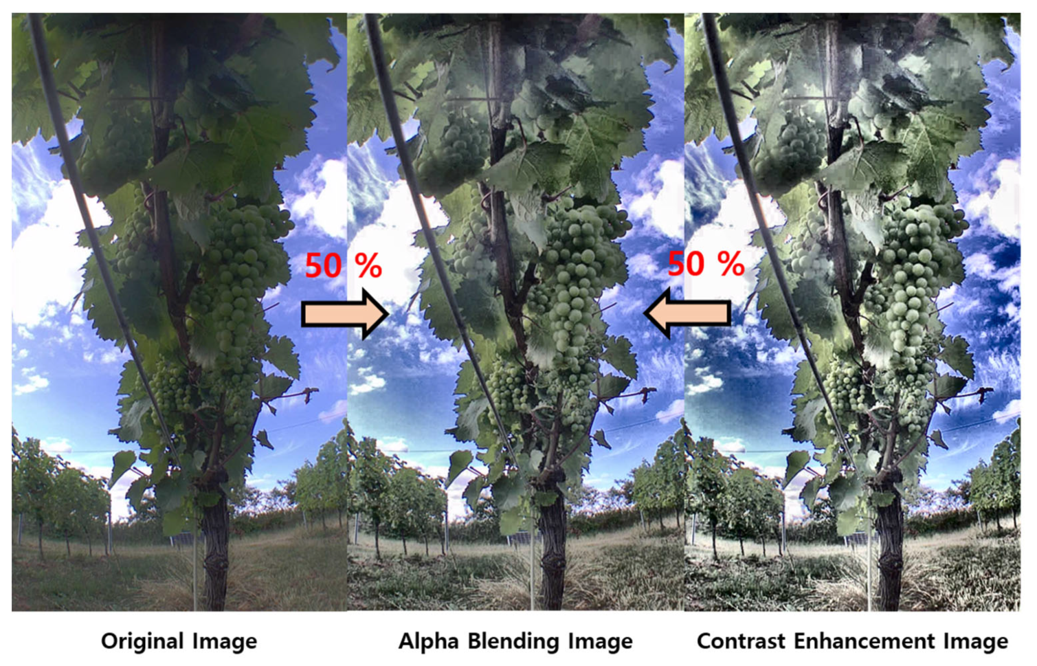
3.2. Optimal Image Data Generation

When the optimal value is obtained, the following image generation process is performed: (1) when the original image is input, non-uniform pixel values are evenly adjusted and Gaussian blur processing is performed to mitigate noise; (2) after applying the contrast enhancement technique (CLAHE) to the L (luminosity) channel of the lab channel using the optimal ‘cliplimit’ value, it is converted to the RGB channel again; (3) the brightness is increased according to the optimal ‘α’ value for the contrast-enhanced image; (4) the saturation arithmetic is applied to the contrast-enhanced image to maintain image quality by preventing the brightness or color values of the image data from changing too much; (5) the image is overlaid with the saturation arithmetic by applying alpha blending to the original image.

Alpha blending is a display method that mixes the background RGB value and the RGB value above it by assigning a new value called ‘Alpha’ to the computer’s color expression value ‘RGB’ for a light effect when another image is overlaid on top of the image. Alpha blending is applied because in the case of an image to which a simple contrast enhancement technique is applied, pixels are often damaged to improve contrast, resulting in noise areas and degrading data quality.

In this paper, alpha blending was applied to the original image and the contrast-enhanced image by specifying a ratio of 0.5, and through Figure 6 it can be seen with the naked eye that the degree of image damage is reduced when alpha blending is applied.

The core goal of the algorithm proposed in this paper is to improve problem areas caused by light or lighting conditions and improve quality by preserving similarity to the original image while minimizing pixel damage. This has the effect of overcoming the disadvantages of existing image contrast enhancement technologies, which require the setting of appropriate hyperparameters because the contrast of input image data varies depending on the lighting environment.

Figure 7 shows the resulting image at each stage of optimal image creation. As the creation stage progresses, the changes between the input and the results can be checked.

3.3. Quality and Similarity Assessment

The generated optimal image may look improved to the naked eye, but it is not completely free from noise and image quality loss, which are chronic problems of contrast enhancement techniques. Therefore, it is necessary to evaluate quality and similarity through a comparison with the original image. In this quality verification and similarity evaluation step, PSNR and SSIM, which are representative IQA algorithms, and LoFTR, a feature point matching algorithm, are applied.

PSNR (peak signal-to-noise ratio) is an indicator that measures quality by calculating the mean square error between the original image and the compressed image. It is mainly used when evaluating image quality loss information in image or video lossy compression and is expressed in decibels (db) [53].

$$\mathrm{P}\mathrm{S}\mathrm{N}\mathrm{R}=10\log \frac{S^2}{MSE}$$

(3)

In Equation (3), MSE (mean square error) is a value obtained by taking an average of the square errors, and S is the maximum value of a pixel. The higher the PSNR value, the lower the loss compared with the original video. In this paper, only images over 25 db were evaluated as optimal images [54].

SSIM (structural similarity index measure) is a method devised to evaluate the difference according to human visual quality rather than numerical error, and it compares the similarity of two images using three elements: luminance, contrast, and structure [55].

$$\begin{gathered} \mathrm{S}\mathrm{S}\mathrm{I}\mathrm{M}\left(x,y\right)=\mathrm{l}{\left(x,y\right)}^{\alpha }·c{\left(x,y\right)}^{\beta }·s{\left(x,y\right)}^{\gamma } \\ =\frac{\left(2{\mu }_x{\mu }_y+C_1\right)\left(2{\sigma }_{xy}+C_2\right)}{\left({\mu }_x^2+{\mu }_y^2+C_1\right)\left({\sigma }_x^2+{\sigma }_y^2+C_2\right)} \end{gathered}$$

(4)

The SSIM value is between 0 and 1, and the closer it is to 1, the higher the similarity. In this paper, only images with SSIM values of 0.75 or higher were evaluated as optimal images. In addition to PSNR and SSIM, there are many types of IQA algorithms, and since the performance, strengths, and weaknesses of each are different, it is good to select an algorithm suitable for the purpose.

LoFTR (detector-free local feature matching with transformers) was used as a feature point matching algorithm. Existing local feature matching methods rely on detecting key points in images, which can be a tricky and computationally expensive task, especially when dealing with low-texture or repetitive regions. On the other hand, LoFTR is an approach to local feature matching in computer vision which uses a transducer-based architecture that does not rely on explicit key point detection, unlike conventional methods.

LoFTR encodes pairs of image patches into feature vectors and predicts the correspondence between them. Unlike density methods, which use cost volumes to find correspondences, LoFTR uses self- and cross-attention layers in the transformer, which conditionally depend on the two images, to obtain a feature descriptor. The global receptive field provided by the transformer allows feature detectors to produce density matches in low-texture regions where it is usually difficult to create repeatable points of interest. The method is trained end-to-end on large datasets and has achieved high performance in experiments on indoor and outdoor datasets. LoFTR is a local feature matching solution that is particularly useful for matching images with low texture or repetitive regions, and it can reduce computational costs and improve the accuracy of the matching process.

$$\mathrm{M}\mathrm{a}\mathrm{t}\mathrm{c}\mathrm{h}\mathrm{i}\mathrm{n}\mathrm{g}\mathrm{A}\mathrm{c}\mathrm{c}\mathrm{u}\mathrm{r}\mathrm{a}\mathrm{c}\mathrm{y}=100\times \frac{Count\left(CorrectMatchingPoints\right)}{Count\left(AllMatchingPoints\right)}$$

(5)

Figure 8 is the feature point matching image obtained using LoFTR. When feature point matching was performed on multiple objects, including the same object, using LoFTR, acciracy was measured using Equation 5 and showed high performance, as shown in the results in Figure 8. The accuracy of feature point matching can be determined by dividing the correctly matched feature points by the number of all matched feature points. In this paper, the optimal image was evaluated based on a matching rate accuracy of 95%.

4. Training Datasets and Object Recognition Task Performance

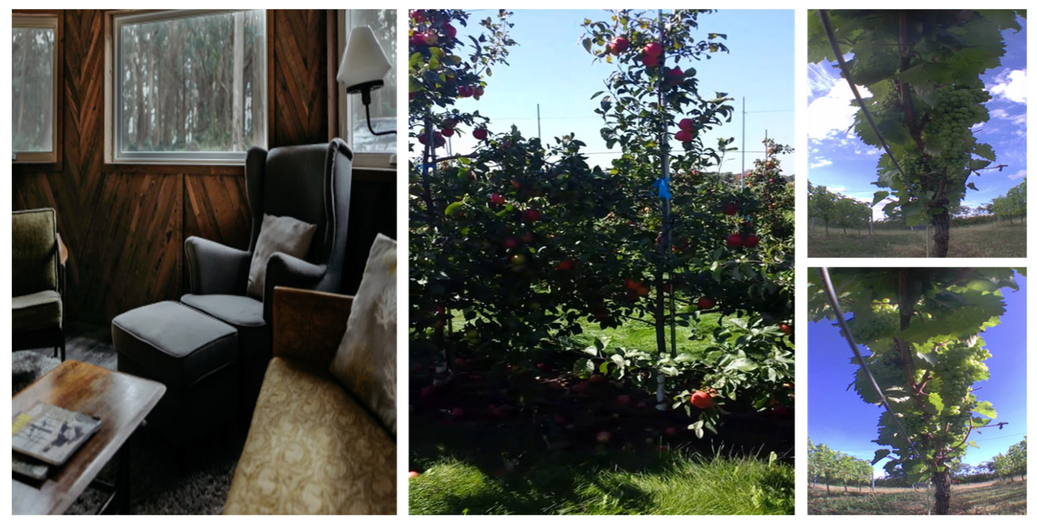
4.1. Training Datasets

Before applying to the task, let us take a look at the datasets to be applied to the experiment. X-rays, fruit tree data (apples, grapes), and marine deposited waste were selected as datasets to be applied in the experiment.

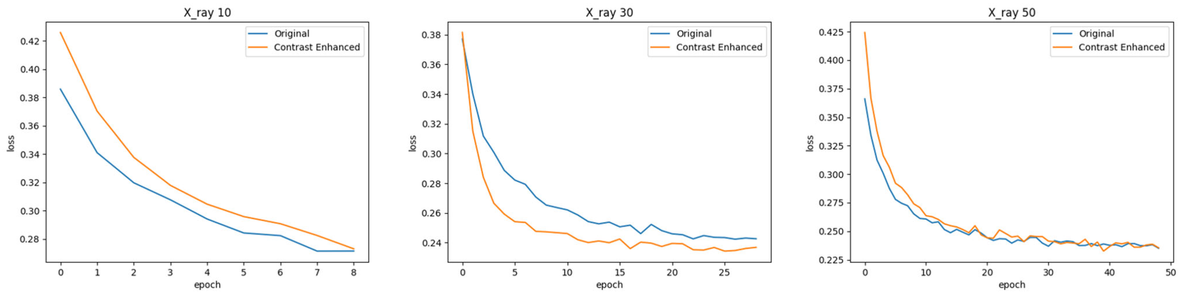
4.1.1. X-ray Dataset

X-ray data were selected because contrast enhancement technology is actively being applied to increase diagnostic accuracy in the medical field, and in this paper, the performance of the classification task was used for measurement [56]. The X-ray dataset consisted of a total of 159,770 images, 512 × 512 in size, and these were divided into 3 classes (COVID-19, pneumonia, normal). The original dataset and preprocessed images were applied.

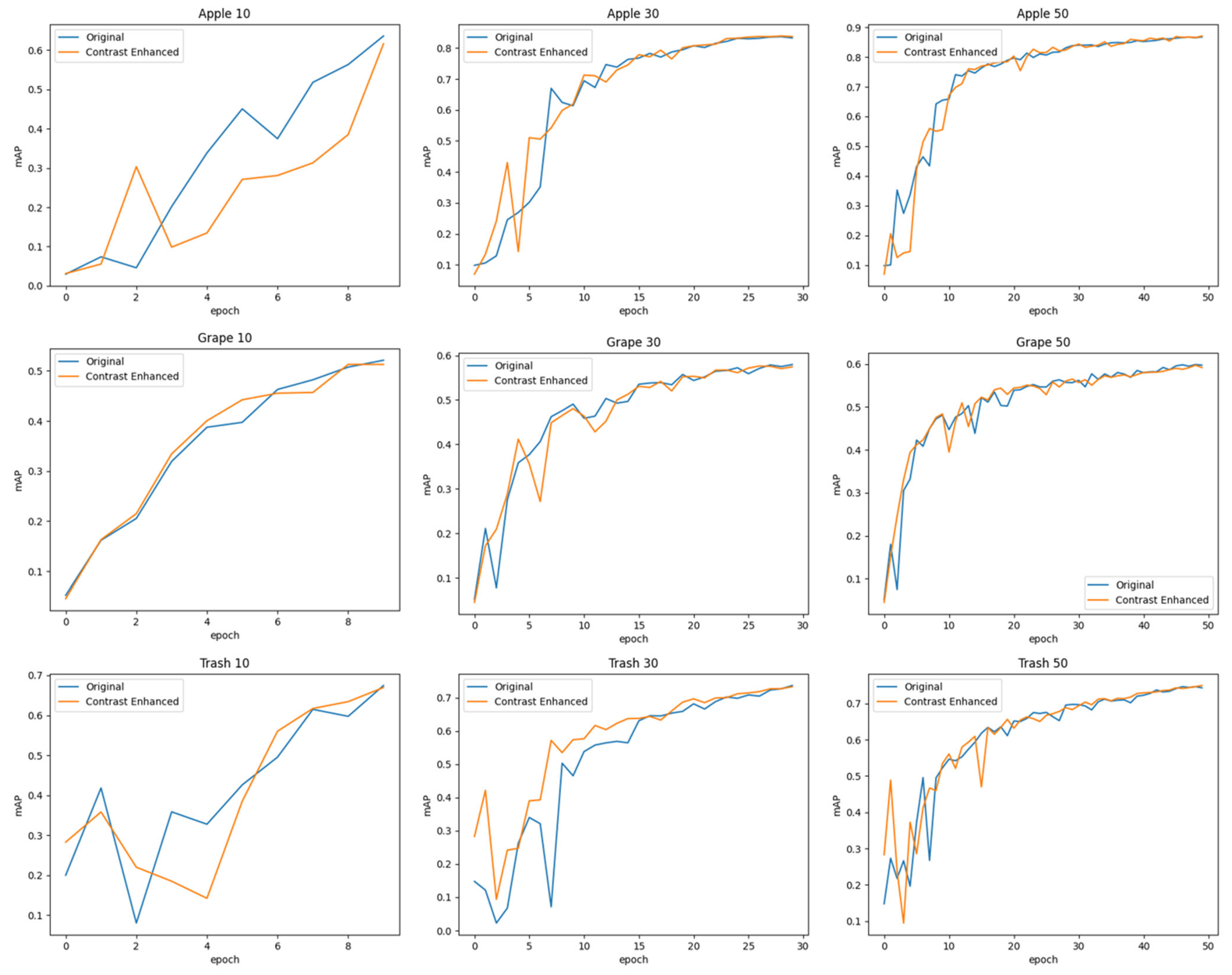
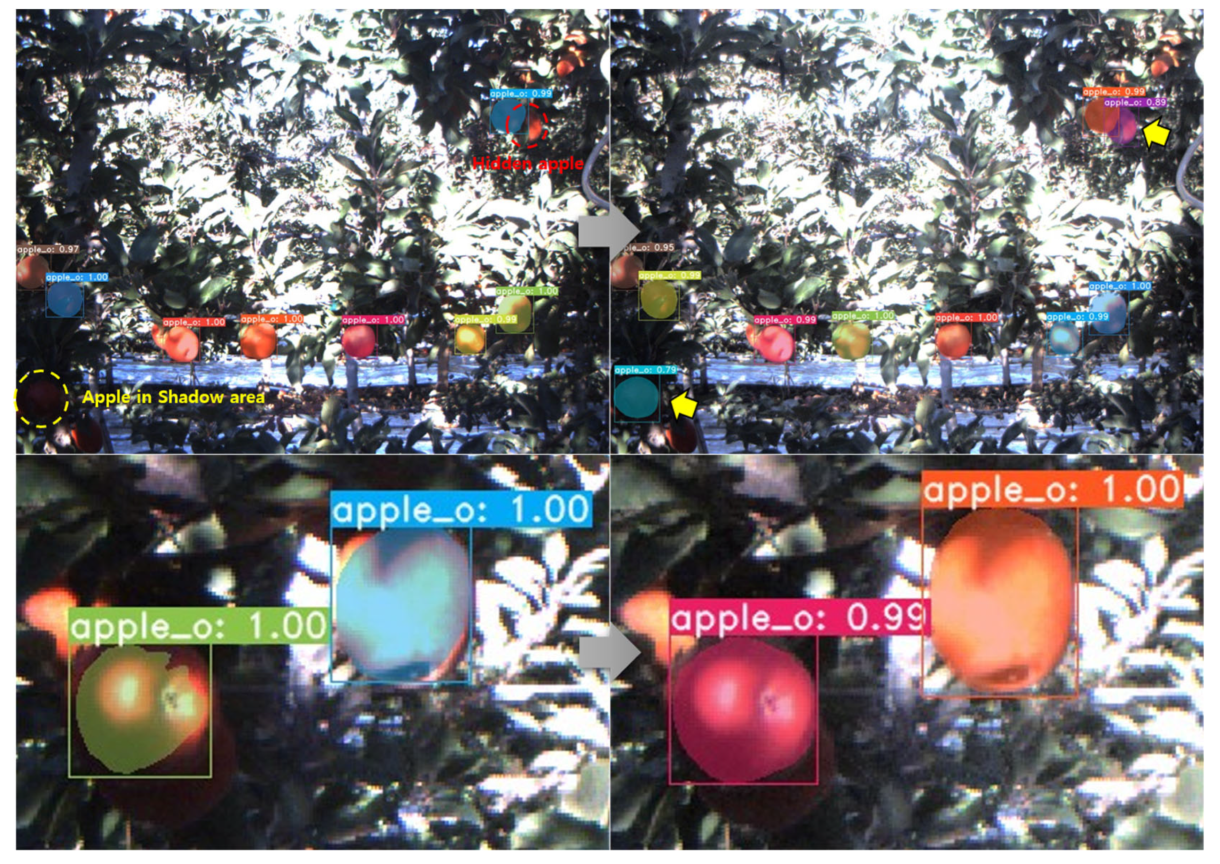
4.1.2. Fruit Tree Dataset

Fruit receives sunlight, and the pulp (the soft inner part of fruit) grows to become a commercial fruit. However, fruit trees sometimes cover their fruits to prevent sunlight from reaching them. In addition, since data may be obtained from fruit trees in many different outdoor environments, object information appears differently by light depending on the position of the sun, and there may be a number of shaded areas, such as shadows. This presents difficulties for object detection and segmentation tasks. The fruit tree dataset is divided into two data types (apples and grapes) and consists of images of a single class of apples and a single class of grapes [57,58]. The apple tree dataset consists of a total of 778 images each of the original dataset and the images with preprocessing applied, and the images are 1280 × 960 in size. The grape tree dataset consists of images to which the original dataset and the preprocessing process were applied. Object detection: 2099 sheets, 1280 × 720 in size.

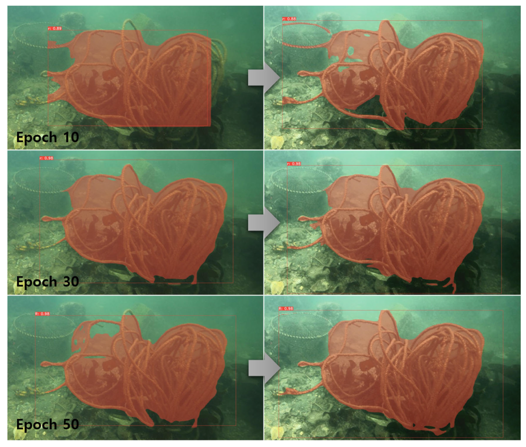
4.1.3. Marine Deposited Waste Dataset

The special and very irregular view in parts of the ocean where light does not enter is often narrow and blurry due to various environmental factors (wind, region, seabed composition, tide, season, ecological environment) [59]. In addition, since most of the long-deposited waste is assimilated by nature, it is difficult to find and predict the size in many cases. This presents difficulties for object detection and segmentation tasks. As one goes deeper, the incoming light decreases and the pressure becomes stronger, so unmanned vehicles such as underwater drones play a role in areas where people cannot go due to increased risk. Since it is very important to measure the exact size of waste in the process of pre-exploration for waste collection, the marine deposited waste dataset was designated as a learning dataset [60]. There are various types of marine deposited waste, but waste fishing gear such as tires, fish traps, rope, and fish nets, which causes great damage to the fishery industry, was selected as a class. The dataset is as follows: object detection: 8781 pieces of the original dataset; instance segmentation: 2689 pieces of the original dataset. The images to which the preprocessing process was applied were 1920 × 1080 in size.

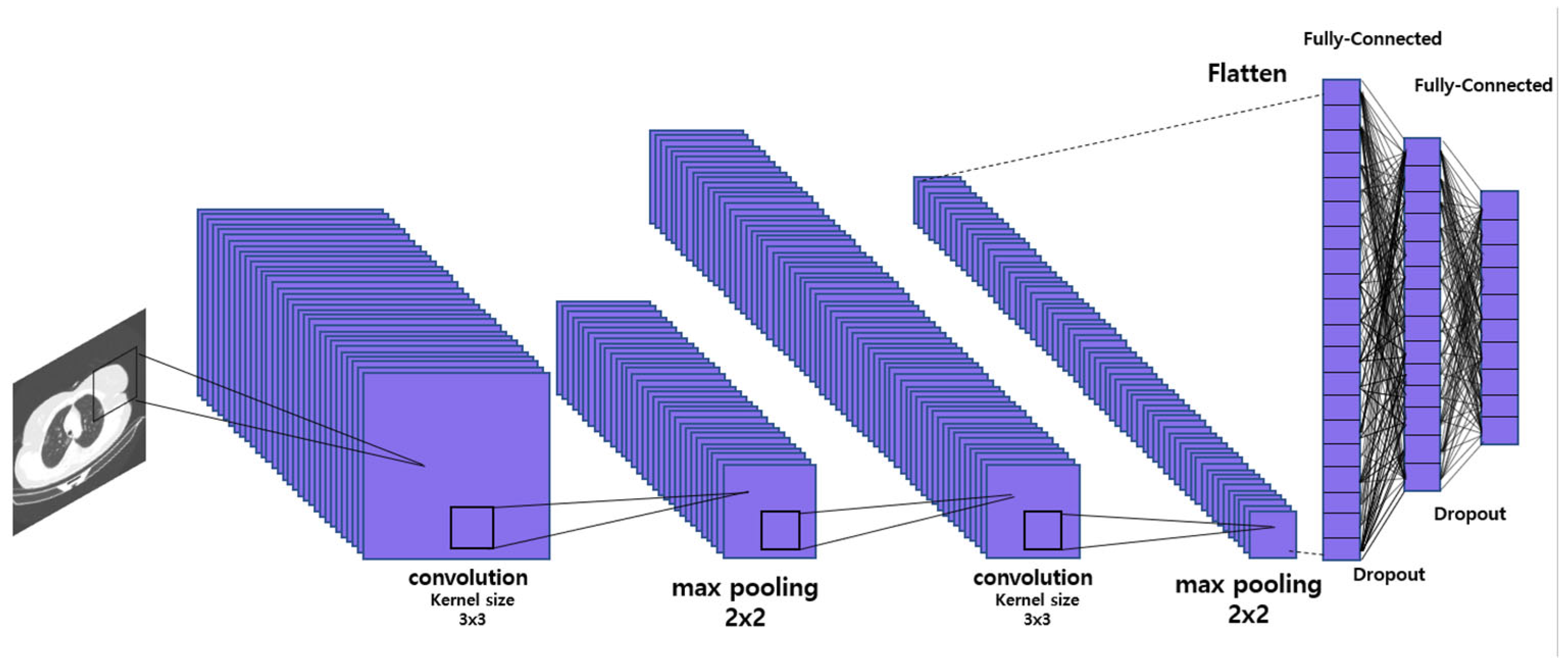
4.2. Classification Task Performance

A convolutional neural network (CNN) was used as a learning model to classify diseases in the X-ray dataset, and the architecture was constructed as shown in Figure 9 [61].

Training was conducted with three epochs (10, 30, 50), a batch size of 256, and a learning rate of 1 × 10⁻⁴.

Figure 10 shows graph images of the X-ray dataset loss by epoch. Through the graphs, we can see that as the epoch increased, the loss steadily decreased. This means that the model’s performance on the training data gradually improved, overfitting or underfitting problems did not occur, and the training data were sufficient and diverse, enabling the model to express the training data appropriately. This shows that the appropriate learning rate was set.

Table 1. CNN model training accuracy for original and contrast-enhanced X-ray dataset.

	Original Dataset	Contrast-Enhanced
Epoch 10	99.48%	99.47%
Epoch 30	99.9%	99.92%
Epoch 50	99.92%	99.94%

shows the accuracy with which the model diagnosed 30,000 test images, which is 20% of the dataset, based on the learned result weights. During the test process, both the original and contrast-enhanced datasets achieved the best performance, and as the epoch increased, the accuracy of the contrast-enhanced dataset improved. Although we achieved over 99% accuracy with 10 epochs, we attempted to secure reliability in accuracy through follow-up training, and the accuracy improved, albeit slightly. Above all, this suggests that when the preprocessing process proposed in this paper is applied to object tasks, performance does not decrease, and the existing performance can at least be maintained and improved.

The maximum epoch limit was set to 50 because it was based on the application of the same epoch value in the same hardware environment of the deep learning model used in each task. In addition, the performance of the deep learning models increased as the number of epochs increased, but since the size of the learning result weight was also proportional, it consumed a lot of hardware resources (to obtain improved learning results with fewer epochs).

4.3. Object Detection Task Performance

The deep learning model used for the fruit tree (apple, grape) and marine deposited waste datasets was a YOLOv5 model, which are widely used in object detection; specifically, the ‘m’ model was used [62]. The epochs were set to 10, 30, and 50, the batch size was 64, and the image size was set to 640 for training. In the validation and testing process after training, objects were detected based on a confidence threshold of 0.7.

Figure 11 shows that in the case of the grape and marine deposited waste data, the mAP improvement value decreased as the epochs increased. Unlike the apple data, which had a standard round shape, these had an atypical shape, and there were many objects with various shapes, so the mAP improvement tended to be low. As the epochs increased, all three dataset graphs showed mAP values increasing stably, and there was no significant difference in mAP performance between the original and contrast-enhanced dataset.

However, as Figure 12 and Figure 13 show, improved results can be obtained in areas with shadows or low contrast, or in environments with blurred vision. The apple and grape object detection results in Figure 12 show that when detecting based on a confidence threshold of 0.7, one can see improved results, i.e., the detection of apples hidden in the shadow area and grapes located relatively behind. The marine deposited waste object detection results in Figure 13 with improved contrast show that objects can be identified more clearly even with the naked eye, and the object detection predicted value also improved by about 0.7 on average.

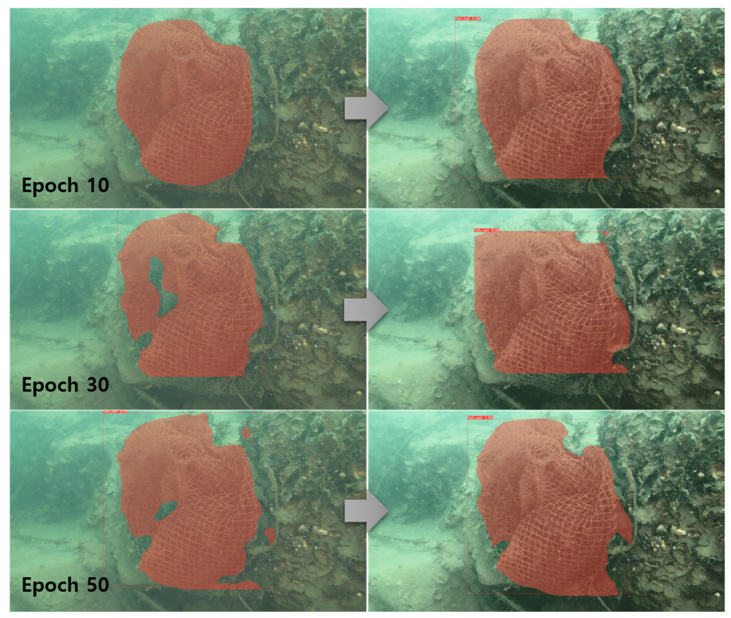
4.4. Instance Segmentation Task Performance

In the segmentation task, You Only Look At CoefficienTs (YOLACT), a real-time instance segmentation model, was used [63]. During the model training process, the epochs was set to 10, 30, and 50, and the batch size was set to 8. In the validation process, top_k (limiting the number of objects in the prediction result) was set to 15 and the confidence threshold was set to 0.7.

Table 2. Mask mAP table according to IoU for each apple object epoch.

Object: Apple	IoU→ Epoch↓	All	50	55	60	65	70	75	80	85	90	95
	10	11.49	26.1	24.42	21.63	17.32	12.85	8.29	3.3	0.93	0.02	0
Original	30	11.05	25.33	23.4	20.61	16.71	12.19	8.1	3.33	0.84	0.02	0
	50	15.2	26.53	25.54	24.38	22.75	20.5	17.53	10.89	3.75	0.17	0
Contrast-Enhanced	10	11.11	25.54	23.95	20.94	17.1	12.15	7.42	3.23	0.79	0.02	0
	30	16.09	27.29	26.58	25.52	24.02	21.61	17.79	12.41	5.33	0.31	0
	50	15.67	25.85	25.48	24.76	23.33	21.76	17.87	12.27	5.06	0.28	0

,

Table 3. Mask mAP table according to IoU for each rope object epoch.

Object: Rope	IoU→ Epoch↓	All	50	55	60	65	70	75	80	85	90	95
	10	2.34	8.72	5.33	3.61	2.28	1.84	1	0.42	0.18	0.02	0
Original	30	6.35	19.19	14.62	10.62	6.84	5.1	3.68	2.17	1.25	0.01	0
	50	6.9	23.26	17.52	12.28	7.68	4.41	2.51	1.03	0.28	0.06	0.01
Contrast-Enhanced	10	2.78	9.44	6.68	5.08	3.09	1.95	1.37	0.15	0.02	0.01	0
	30	6.58	19.46	15.81	11.08	8.09	5.04	3.75	2.07	0.45	0.09	0
	50	6.96	21.36	16.79	11.71	7.44	4.95	3.29	1.85	1.19	0.99	0

and

Table 4. Mask mAP table according to IoU for each fish net object epoch.

Object: Fish Net	IoU→ Epoch↓	All	50	55	60	65	70	75	80	85	90	95
	10	9.94	22.55	22.04	21.03	15.74	9.11	5.93	2.89	0.08	0.08	0
Original	30	14.33	26.55	25.8	24.6	19.03	18.06	16.63	8.84	3.05	0.64	0.07
	50	14.25	28.69	21.89	21.89	19.74	18.94	15.25	9.03	4.57	2.18	0.27
Contrast-Enhanced	10	10.55	26.44	23.22	19.83	13.76	8.05	7.88	4.56	1.66	0.07	0
	30	14.24	28.75	24.38	21.49	19.09	18.78	12.9	11.99	4.53	0.41	0.08
	50	16.58	30.14	28.29	27.54	25.21	19.49	18.23	11.75	4.5	0.54	0.12

are mask mAP tables according to IoU for each epoch of the apple, rope, and fish net objects after training. When comparing the original and contrast-enhanced datasets, it can be seen that the overall difference in mask mAP for each object is not large, and the performance of the contrast-enhanced dataset is relatively high.

Figure 14, Figure 15 and Figure 16 show images of the instance segmentation results for each object. In Figure 14, you can see that in the case of the apples, while maintaining the existing segmentation performance, the apples in the shadow area, or those that are hidden, are captured, and the mask recognition performance is also increased to enable more accurate size prediction. For the rope and fish nets, which have atypical shapes, object size prediction performance improvements were confirmed in in environments with little light and poor viewing conditions through segmentation for each epoch.

5. Conclusions

In this paper, we proposed a contrast enhancement-based preprocessing process which uses the CLAHE algorithm to obtain improved results in object tasks by improving problem areas caused by light or lighting conditions. The preprocessing process extracts the optimal ‘cliplimit’ and ‘additional brightness (α)’ values, generates optimal image data based on these, and then proceeds with the quality and similarity measurement process.

The optimal values refer to the absolute brightness difference between the two images (original and contrast-enhanced) and the maximum value of the variance for sharpness, respectively. The generated image has optimal contrast enhancement and brightness control, making it more suitable and easier to use for object recognition than the original image, and it has a pixel environment more similar to that of the original image than those of the images generated through most contrast enhancement algorithms. Deep learning models used in object recognition tasks rely heavily on learning data, and environmental similarities between learning data and input data can also affect performance. Therefore, the proposed preprocessing process can be used not only for generating learning data, but also as a preprocessing process for input data in the object task process, and experiments were conducted by applying the preprocessing process to learning and input data. Object tasks include classification, detection, and segmentation, and CNN, YOLOv5, and YOLACT models were used for these, respectively. The X-ray, apple, grape, and marine deposited waste datasets were selected as training datasets based on the need for technology to improve contrast. As a result of the experiment, the performance of the original datasets was high in three tasks. However, when comparing the object task performance of the original dataset with that of the contrast-enhanced datasets to which this paper’s preprocessing process was applied, improvements were observed in areas such as shadows or contrast phenomena while the existing performance was maintained or improved. In the classification task, the average accuracy was slightly improved, and in the object detection task, additional objects were detected in shadows or low-light areas and the detection rate was improved. In the segmentation task, the size of the object was segmented more accurately than in the original dataset. Through this, it will be possible to improve results not only for the dataset used in this paper, but also for datasets that require contrast enhancement. The proposed preprocessing process builds a similar environment through improved learning data and input data in the object recognition task process, and it suggests that more accurate results can be obtained.

In future research, we plan to study preprocessing process optimization and application methods that can be applied to hardware that requires low resources, such as robots and unmanned vehicles.

References

1. Paul, N.; Chung, C. Application of HDR algorithms to solve direct sunlight problems when autonomous vehicles using machine vision systems are driving into sun. Comput. Ind. 2018, 98, 192–196. [Google Scholar] [CrossRef]
2. Gray, R.; Regan, D. Glare susceptibility test results correlate with temporal safety margin when executing turns across approaching vehicles in simulated low-sun conditions. OPO 2007, 27, 440–450. [Google Scholar] [CrossRef] [PubMed]
3. Ning, Y.; Jin, Y.; Peng, Y.D.; Yan, J. Low illumination underwater image enhancement based on nonuniform illumination correction and adaptive artifact elimination. Front. Mar. Sci. 2023, 10, 1–15. [Google Scholar] [CrossRef]
4. An Investigation of Videos for Crowd Analysis. Available online: https://shodhganga.inflibnet.ac.in:8443/jspui/handle/10603/480375 (accessed on 1 March 2023).
5. Yu, C.; Li, S.; Feng, W.; Zheng, T.; Liu, S. SACA-fusion: A low-light fusion architecture of infrared and visible images based on self-and cross-attention. Vis. Comput. 2023, 1, 1–10. [Google Scholar] [CrossRef]
6. Wu, Y.; Wang, L.; Zhang, L.; Bai, Y.; Cai, Y.; Wang, S.; Li, Y. Improving autonomous detection in dynamic environments with robust monocular thermal SLAM system. ISPRS J. Photogramm. Remote Sens. 2023, 203, 265–284. [Google Scholar] [CrossRef]
7. Shareef, A.A.A.; Yannawar1, P.L.; Abdul-Qawy, A.S.H.; Al-Nabhi, H.; Bankar, R.B. Deep Learning Based Model for Fire and Gun Detection. In Proceedings of the First International Conference on Advances in Computer Vision and Artificial Intelligence Technologies (ACVAIT 2022), Aurangabad, India, 1–2 August 2022; Atlantis Press: Amsterdam, The Netherlands, 2023; pp. 422–430. [Google Scholar] [CrossRef]
8. Parez, S.; Dilshad, N.; Alghamdi, N.S.; Alanazi, T.M.; Lee, J.W. Visual Intelligence in Precision Agriculture: Exploring Plant Disease Detection via Efficient Vision Transformers. Sensors 2023, 23, 6949. [Google Scholar] [CrossRef]
9. Fan, C.; Su, Q.; Xiao, Z.; Su, H.; Hou, A.; Luan, B. ViT-FRD: A Vision Transformer Model for Cardiac MRI Image Segmentation Based on Feature Recombination Distillation. IEEE Access 2023, 1, 1. [Google Scholar] [CrossRef]
10. Moreno, H.; Gómez, A.; Altares-López, S.; Ribero, A.; Andujar, D. Analysis of Stable Diffusion-Derived Fake Weeds Performance for Training Convolutional Neural Networks. SSRN 2023, 1, 1–27. [Google Scholar] [CrossRef]
11. Bi, L.; Buehner, U.; Fu, X.; Williamson, T.; Choong, P.F.; Kim, J. Hybrid Cnn-Transformer Network for Interactive Learning of Challenging Musculoskeletal Images. SSRN 2023, 1, 1–21. [Google Scholar] [CrossRef]
12. Parsons, M.H.; Stryjek, R.; Fendt, M.; Kiyokawa, Y.; Bebas, P.; Blumstein, D.T. Making a case for the free exploratory paradigm: Animal welfare-friendly assays that enhance heterozygosity and ecological validity. Front. Behav. Neurosci. 2023, 17, 1–8. [Google Scholar] [CrossRef]
13. Majid, H.; Ali, K.H. Automatic Diagnosis of Coronavirus Using Conditional Generative Adversarial Network (CGAN). Iraqi J. Sci. 2023, 64, 4542–4556. [Google Scholar] [CrossRef]
14. Lee, J.; Seo, K.; Lee, H.; Yoo, J.E.; Noh, J. Deep Learning-Based Lighting Estimation for Indoor and Outdoor. J. Korea Comput. Graph. Soc. 2021, 27, 31–42. [Google Scholar] [CrossRef]
15. Hawlader, F.; Robinet, F.; Frank, R. Leveraging the Edge and Cloud for V2X-Based Real-Time Object Detection in Autonomous Driving. arXiv 2023, arXiv:2308.05234. [Google Scholar]
16. Lin, T.; Huang, G.; Yuan, X.; Zhong, G.; Huang, X.; Pun, C.M. SCDet: Decoupling discriminative representation for dark object detection via supervised contrastive learning. Vis. Comput 2023. [Google Scholar] [CrossRef]
17. Chen, W.; Shah, T. Exploring low-light object detection techniques. arXiv 2021, arXiv:2107.14382. [Google Scholar]
18. Jägerbrand, A.K.; Sjöbergh, J. Effects of weather conditions, light conditions, and road lighting on vehicle speed. SpringerPlus 2016, 5, 505. [Google Scholar] [CrossRef]
19. Nandal, A.; Bhaskar, V.; Dhaka, A. Contrast-based image enhancement algorithm using grey-scale and colour space. IET Signal Process. 2018, 12, 514–521. [Google Scholar] [CrossRef]
20. Pizer, S.M. Intensity mappings to linearize display devices. Comput. Graph. Image Process. 1981, 17, 262–268. [Google Scholar] [CrossRef]
21. Mukhopadhyay, S.; Chanda, B. A multiscale morphological approach to local contrast enhancement. Signal Process. 2000, 80, 685–696. [Google Scholar] [CrossRef]
22. Hum, Y.C.; Lai, K.W.; Mohamad Salim, M.I. Multiobjectives bihistogram equalization for image contrast enhancement. Complexity 2014, 20, 22–36. [Google Scholar] [CrossRef]
23. Pizer, S.M.; Amburn, E.P.; Austin, J.D.; Cromartie, R.; Geselowitz, A.; Greer, T.; ter Haar Romeny, B.; Zimmerman, J.B.; Zuiderveld, K. Adaptive histogram equalization and its variations. Comput. Vis. Graph. Image Process. 1987, 39, 355–368. [Google Scholar] [CrossRef]
24. Zuiderveld, K. Contrast limited adaptive histogram equalization. In Graphical Gems IV; Academic Press Professional, Inc.: San Diego, CA, USA, 1994; pp. 474–485. [Google Scholar]
25. Kim, J.I.; Lee, J.W.; Honga, S.H. A Method of Histogram Compression Equalization for Image Contrast Enhancement. In Proceedings of the 2013 39th Korea Information Processing Society Conference, Busan, Republic of Korea, 10–11 May 2013; Volume 20, pp. 346–349. [Google Scholar]
26. Li, G.; Yang, Y.; Qu, X.; Cao, D.; Li, K. A deep learning based image enhancement approach for autonomous driving at night. Knowl. Based Syst. 2021, 213, 106617. [Google Scholar] [CrossRef]
27. Chen, Z.; Pawar, K.; Ekanayake, M.; Pain, C.; Zhong, S.; Egan, G.F. Deep learning for image enhancement and correction in magnetic resonance imaging—State-of-the-art and challenges. J. Digit. Imaging 2023, 36, 204–230. [Google Scholar] [CrossRef]
28. Wang, Z.; Bovik, A.C.; Lu, L. Why is image quality assessment so difficult? In Proceedings of the 2002 IEEE International Conference on Acoustics, Speech, and Signal Processing (ICASSP), Orlando, FL, USA, 13–17 May 2002; Volume 4, p. IV–3313. [Google Scholar] [CrossRef]
29. Wang, L. A survey on IQA. arXiv 2021, arXiv:2109.00347. [Google Scholar]
30. Athar, S.; Wang, Z. Degraded reference image quality assessment. IEEE Trans. Image Process. 2023, 32, 822–837. [Google Scholar] [CrossRef] [PubMed]
31. Sheikh, H.R.; Bovik, A.C. A visual information fidelity approach to video quality assessment. In Proceedings of the First International Workshop on Video Processing and Quality Metrics for Consumer Electronics, Scottsdale, AZ, USA; 2005; Volume 7, pp. 2117–2128. [Google Scholar]
32. Larson, E.C.; Chandler, D.M. Most apparent distortion: A dual strategy for full-reference image quality assessment. Image Qual. Syst. Perform. VI 2009, 7242, 270–286. [Google Scholar] [CrossRef]
33. Zhang, L.; Zhang, L.; Mou, X.; Zhang, D. FSIM: A feature similarity index for image quality assessment. IEEE Trans. Image Process. 2011, 20, 2378–2386. [Google Scholar] [CrossRef]
34. Liu, A.; Lin, W.; Narwaria, M. Image quality assessment based on gradient similarity. IEEE Trans. Image Process. 2011, 21, 1500–1512. [Google Scholar] [CrossRef]
35. Xue, W.; Zhang, L.; Mou, X.; Bovik, A.C. Gradient magnitude similarity deviation: A highly efficient perceptual image quality index. IEEE Trans. Image Process. 2013, 23, 684–695. [Google Scholar] [CrossRef]
36. Mittal, A.; Moorthy, A.K.; Bovik, A.C. Blind/referenceless image spatial quality evaluator. In Proceedings of the 2011 Conference record of the Forty Fifth Asilomar Conference on Signals, Systems and Computers (ASILOMAR), Pacific Grove, CA, USA, 6–9 November 2011; pp. 723–727. [Google Scholar] [CrossRef]
37. Lin, H.; Hosu, V.; Saupe, D. DeepFL-IQA: Weak supervision for deep IQA feature learning. arXiv 2020, arXiv:2001.08113. [Google Scholar]
38. Ding, K.; Ma, K.; Wang, S.; Simoncelli, E.P. Image quality assessment: Unifying structure and texture similarity. IEEE Trans. Pattern Anal. Mach. Intell. 2020, 44, 2567–2581. [Google Scholar] [CrossRef] [PubMed]
39. Lowe, D.G. Distinctive image features from scale-invariant keypoints. Int. J. Comput. Vis. 2004, 60, 91–110. [Google Scholar] [CrossRef]
40. Bay, H.; Ess, A.; Tuytelaars, T.; Van Gool, L. Speeded-up robust features (SURF). Comput. Vis. Image Underst. 2008, 110, 346–359. [Google Scholar] [CrossRef]
41. Rublee, E.; Rabaud, V.; Konolige, K.; Bradski, G. ORB: An efficient alternative to SIFT or SURF. In Proceedings of the 2011 International Conference on Computer Vision (ICCV), Barcelona, Spain, 6–13 November 2011; pp. 2564–2571. [Google Scholar] [CrossRef]
42. DeTone, D.; Malisiewicz, T.; Rabinovich, A. Superpoint: Self-supervised interest point detection and description. In Proceedings of the IEEE Conference on Computer Vision and Pattern Recognition Workshops (CVPRW), Salt Lake City, UT, USA, 18–22 June 2018; pp. 224–236. [Google Scholar] [CrossRef]
43. Dusmanu, M.; Rocco, I.; Pajdla, T.; Pollefeys, M.; Sivic, J.; Torii, A.; Sattler, T. D2-net: A trainable cnn for joint detection and description of local features. arXiv 2019, arXiv:1905.03561. [Google Scholar] [CrossRef]
44. Ono, Y.; Trulls, E.; Fua, P.; Yi, K.M. LF-Net: Learning local features from images. Adv. Neural Inf. Process. Syst. 2018, 31, 1–11. [Google Scholar]
45. Revaud, J.; Weinzaepfel, P.; De Souza, C.; Pion, N.; Csurka, G.; Cabon, Y.; Humenberger, M. R2D2: Repeatable and reliable detector and descriptor. arXiv 2019, arXiv:1906.06195. [Google Scholar] [CrossRef]
46. Cover, T.; Hart, P. Nearest neighbor pattern classification. IEEE Trans. Inf. Theory 1967, 13, 21–27. [Google Scholar] [CrossRef]
47. Bhatia, N. Survey of nearest neighbor techniques. arXiv 2010, arXiv:1007.0085. [Google Scholar] [CrossRef]
48. Muja, M.; Lowe, D.G. Fast approximate nearest neighbors with automatic algorithm configuration. In Proceedings of the 4th International Conference on Computer Vision Theory and Applications (VISAPP), Lisboa, Portugal, 5–8 February 2009; Volume 1, pp. 331–340. [Google Scholar]
49. Zagoruyko, S.; Komodakis, N. Deep compare: A study on using convolutional neural networks to compare image patches. Comput. Vis. Image Underst. 2017, 164, 38–55. [Google Scholar] [CrossRef]
50. Sarlin, P.E.; DeTone, D.; Malisiewicz, T.; Rabinovich, A. Superglue: Learning feature matching with graph neural networks. In Proceedings of the IEEE/CVF Conference on Computer Vision and Pattern Recognition (CVPR), Seattle, WA, USA, 13–19 June 2020; pp. 4938–4947. [Google Scholar]
51. Luo, Z.; Shen, T.; Zhou, L.; Zhu, S.; Zhang, R.; Yao, Y.; Tian, F.; Quan, L. Geodesc: Learning local descriptors by integrating geometry constraints. In Proceedings of the European Conference on Computer Vision (ECCV), Munich, Germany, 8–14 September 2018; pp. 170–185. [Google Scholar] [CrossRef]
52. Woldamanuel, E.M. Grayscale Image Enhancement Using Water Cycle Algorithm. IEEE Access 2023, 11, 86575–86596. [Google Scholar] [CrossRef]
53. Johnson, D.H. Signal-to-noise ratio. Scholarpedia 2006, 1, 2088. [Google Scholar] [CrossRef]
54. Juneja, S.; Anand, R. Contrast Enhancement of an Image by DWT-SVD and DCT-SVD. In Data Engineering and Intelligent Computing: Proceedings of IC3T 2016, Proceedings of the Third Springer International Conference on Computer & Communication Technologies, Andhra Pradesh, India, 28–29 October 2016; Springer: Singapore, 2018; pp. 595–603. [Google Scholar] [CrossRef]
55. Wang, Z.; Bovik, A.C.; Sheikh, H.R.; Simoncelli, E.P. Image quality assessment: From error visibility to structural similarity. IEEE Trans. Image Process. 2004, 13, 600–612. [Google Scholar] [CrossRef] [PubMed]
56. Gunraj, H.; Sabri, A.; Koff, D.; Wong, A. COVID-Net CT-2: Enhanced deep neural networks for detection of COVID-19 from chest CT images through bigger, more diverse learning. Front. Med. 2022, 8, 729287. [Google Scholar] [CrossRef] [PubMed]
57. Häni, N.; Roy, P.; Isler, V. MinneApple: A benchmark dataset for apple detection and segmentation. IEEE Robot. Autom. Lett. 2020, 5, 852–858. [Google Scholar] [CrossRef]
58. Santos, T.; De Souza, L.; Dos Santos, A.; Sandra, A. Embrapa Wine Grape Instance Segmentation Dataset–Embrapa WGISD. Zenodo 2019. [Google Scholar] [CrossRef]
59. Chen, X.; Yuan, M.; Fan, C.; Chen, X.; Li, Y.; Wang, H. Research on an Underwater Object Detection Network Based on Dual-Branch Feature Extraction. Electronics 2023, 12, 3413. [Google Scholar] [CrossRef]
60. Image of Marine Sediment Trash. Available online: https://www.aihub.or.kr/ (accessed on 18 June 2021).
61. Simard, P.Y.; Steinkraus, D.; Platt, J.C. Best practices for convolutional neural networks applied to visual document analysis. In Proceedings of the Seventh International Conference on Document Analysis and Recognition, Edinburgh, UK, 6 August 2003; Volume 3. [Google Scholar]
62. Kim, P.; Huang, X.; Fang, Z. SSD PCB Component Detection Using YOLOv5 Model. J. Inf. Commun. Converg. Eng. 2023, 21, 24–31. [Google Scholar] [CrossRef]
63. Bolya, D.; Zhou, C.; Xiao, F.; Lee, Y.J. Yolact: Real-time instance segmentation. In Proceedings of the IEEE/CVF International Conference on Computer Vision (ICCV), Seoul, Republic of Korea, 27 October–2 November 2019; pp. 9157–9166. [Google Scholar]
Figure 1. Example image showing problem caused by light both indoors and outdoors.
Applsci 13 10760 g001
Figure 2. Diagram of preprocessing process.
Applsci 13 10760 g002
Figure 3. Preprocessing process flow chart.
Applsci 13 10760 g003
Figure 4. Example image showing absolute brightness difference and cliplimit optimal value.
Applsci 13 10760 g004
Figure 5. Example image of sharpness and ‘α’ (additional brightness) optimal value obtained via edge-detection.
Applsci 13 10760 g005
Figure 6. Original image, alpha blending image, and contrast enhancement image.
Applsci 13 10760 g006
Figure 7. Step-by-step optimal image data generation images.
Applsci 13 10760 g007
Figure 8. Feature point matching image obtained using LoFTR.
Applsci 13 10760 g008
Figure 9. CNN Architecture.
Applsci 13 10760 g009
Figure 10. X-ray loss graphs.
Applsci 13 10760 g010
Figure 11. mAP graphs of the results after training the object detection model.
Applsci 13 10760 g011
Figure 12. Images of improved apple and grape object detection results (epoch 30).
Applsci 13 10760 g012
Figure 13. Images of improved marine deposited waste object detection results (epoch 50).
Applsci 13 10760 g013
Figure 14. Images of apple instance segmentation results (epoch 50).
Applsci 13 10760 g014
Figure 15. Images of rope instance segmentation results.
Applsci 13 10760 g015
Figure 16. Images of fish net instance segmentation results.
Applsci 13 10760 g016