Individual parts of the project structure and their applications, physical devices, and creation will be presented in detail in the next section.
3.1. Automation of Production Processes
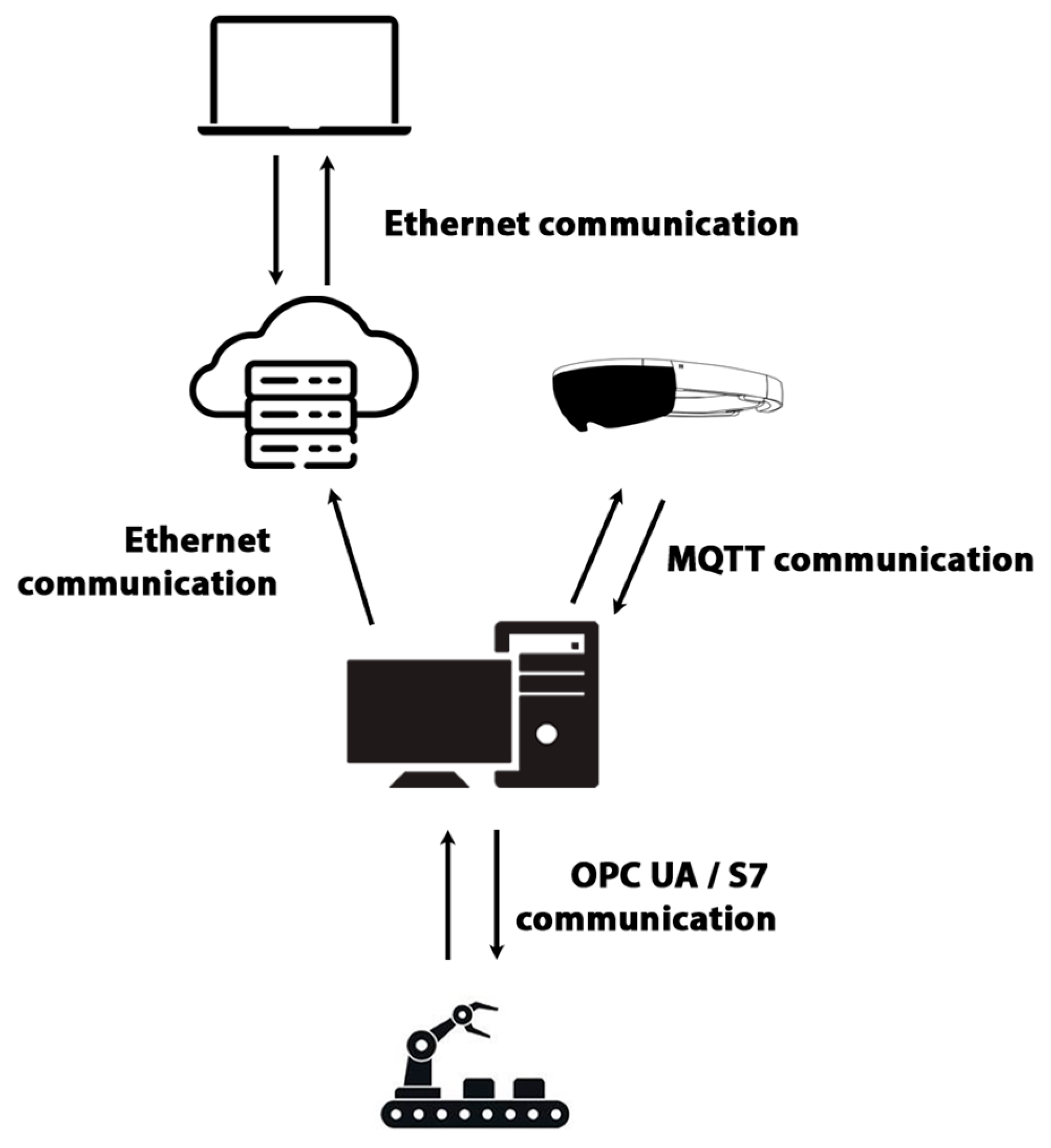
An important part of the project was the appropriate selection of laboratory production models and PLC devices. We chose PLC devices from Siemens. They provide communication using their own S7 protocol on the devices and communication using the OPC UA protocol on higher models (S7-1500 and some S7-1200) [
29].
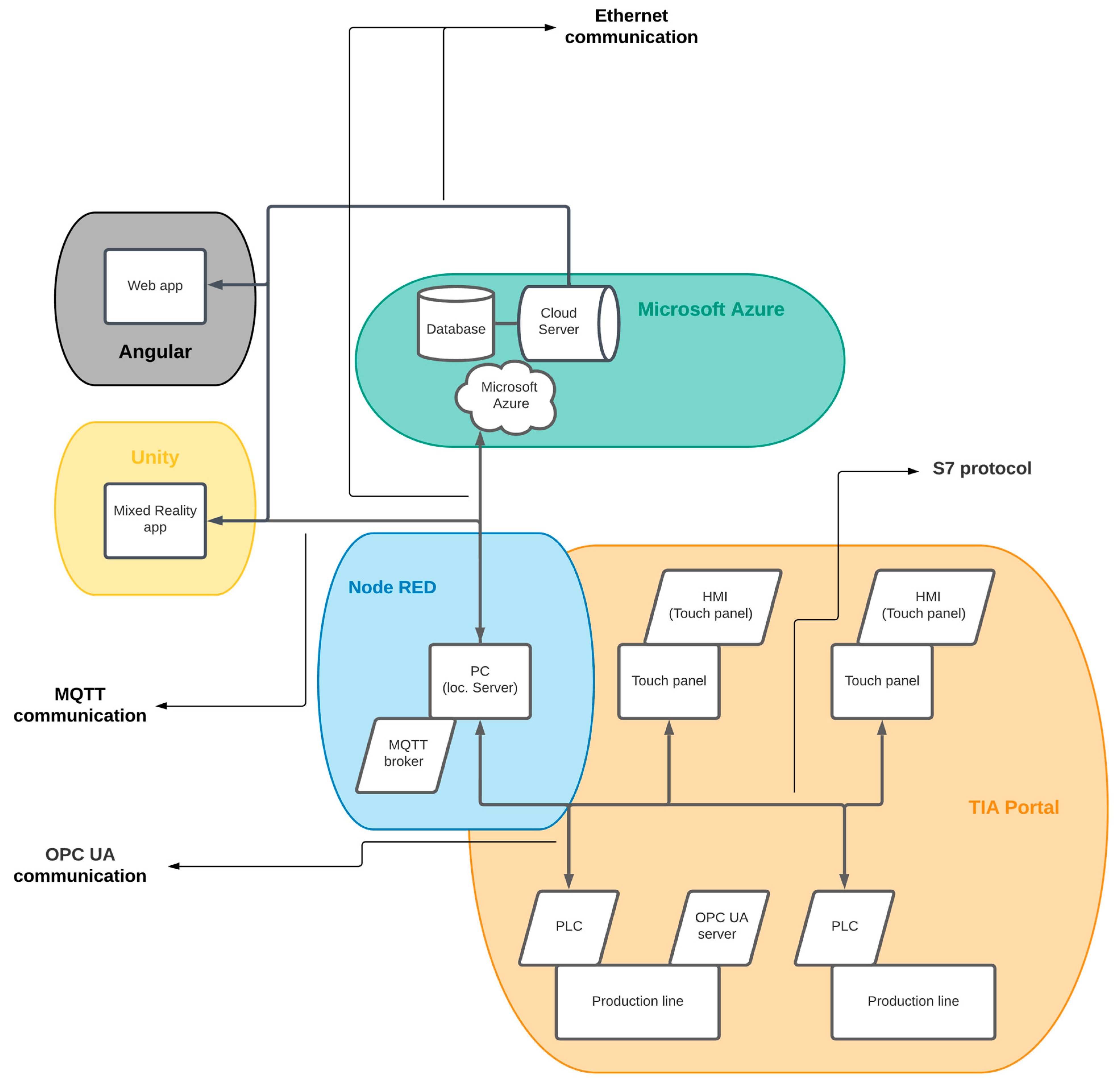
When designing the platform (system), we proceeded in accordance with the principles of Industry 4.0. In this case, we require the proposed system to be modular. Therefore, we chose communication using the OPC UA protocol, which is also compatible with devices from other manufacturers. Two laboratory models of production systems are used for testing, so we decided to use both protocols to verify modularity: one model will use the S7 protocol and the other will use the OPC UA protocol.
As already mentioned, both laboratory models are automated using Siemens PLC equipment and each of them contains a touch screen Siemens HMI KTP 700 Basic [
30] for controlling the model and displaying its data.
All devices communicate at the level of a local network without access to the Internet. The devices can communicate with each other, but, since they are two separate systems, the communication will take place between the PLC device, the HMI device of the given laboratory model, and the local server.
In the proposed solution, we use educational models from Fischertechnik [
21,
31] as production models. Individual laboratory production models, their visualization, and their functionality are described in detail in the next section.
3.1.1. Production Line Model
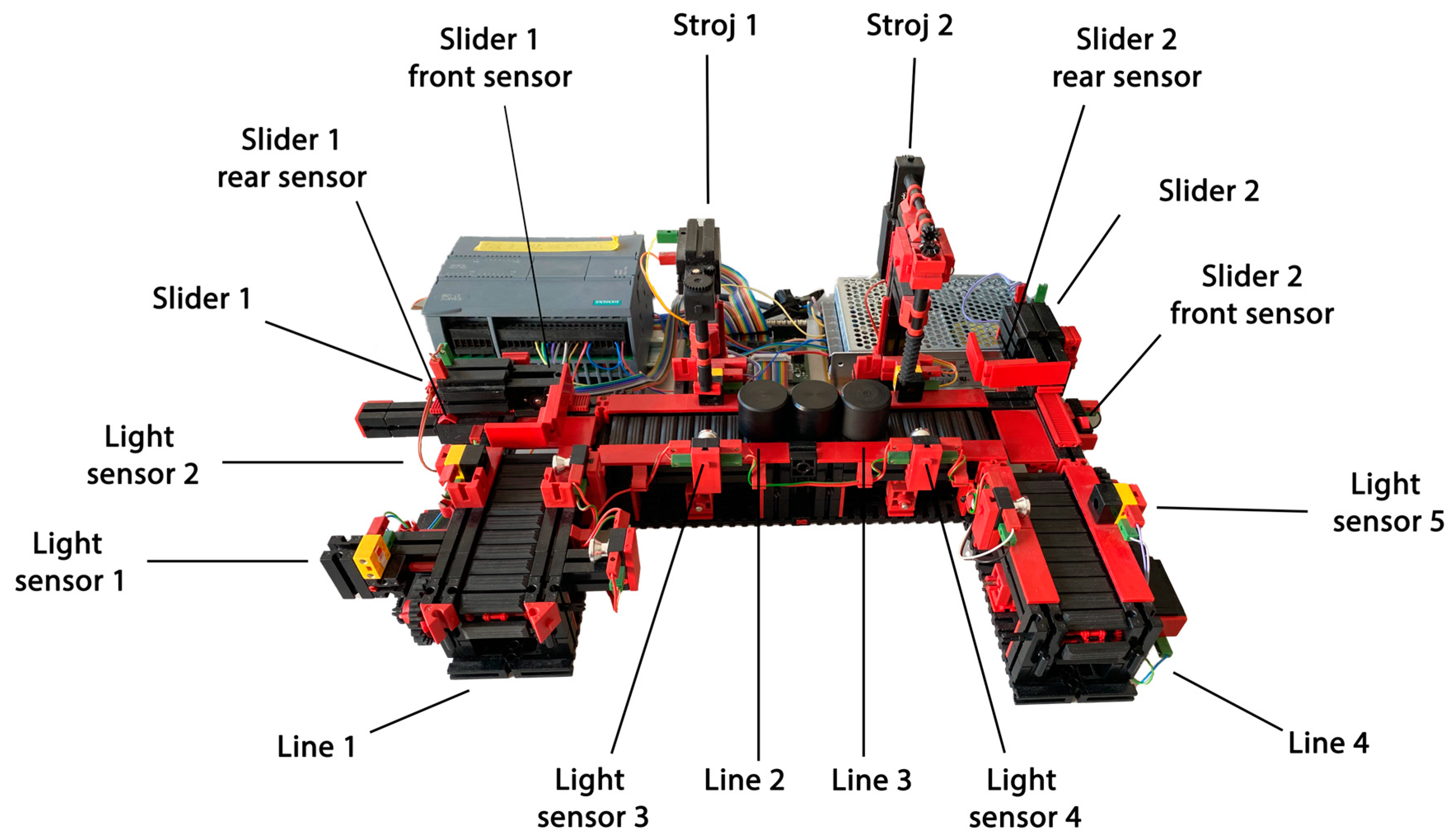
The first laboratory production model is the U-shaped production line model (hereafter referred to as model 1). The production line model represents the process where products are processed by two machines. The model consists of four belts, two machine tools, and two sliders, with both sliders allowing forward and backward movement. Five light sensors are available to detect the position of the product in the production process. To detect the positions of the sliders, the model is equipped with four end sensors (two rear and two front). All the listed components of the laboratory production model are marked in
Figure 5.
A smaller PLC device, model S7 1215C DC/DC/DC, was used to control this model. A PLC device of this type contains 14 digital inputs, 10 digital outputs, and 2 analog outputs. For the automation of this system, 9 digital inputs and 10 digital outputs were needed.
For this laboratory production model, we compiled an algorithm in the TIA Portal environment, where we designed the processing of the product and its movement through the entire production process. Furthermore, the algorithm contained the following treatments and functionalities:
The treatment of the collision of products on the production line with several products simultaneously located on the production model;
The detection of product loss from the belts: if the next step of the control algorithm is not performed within 5 s, the alarm on the given belt is activated;
Counting engine hours for all belts and machines;
Counting the number of products on the production line and the number of finished products;
The manual resetting of both product numbers;
The possibility of operating the production line in manual and automatic modes;
The start function, a treatment for a quick shutdown of the line in the event of an unexpected collision.
3.1.2. Sorting Line Model with Color Detection
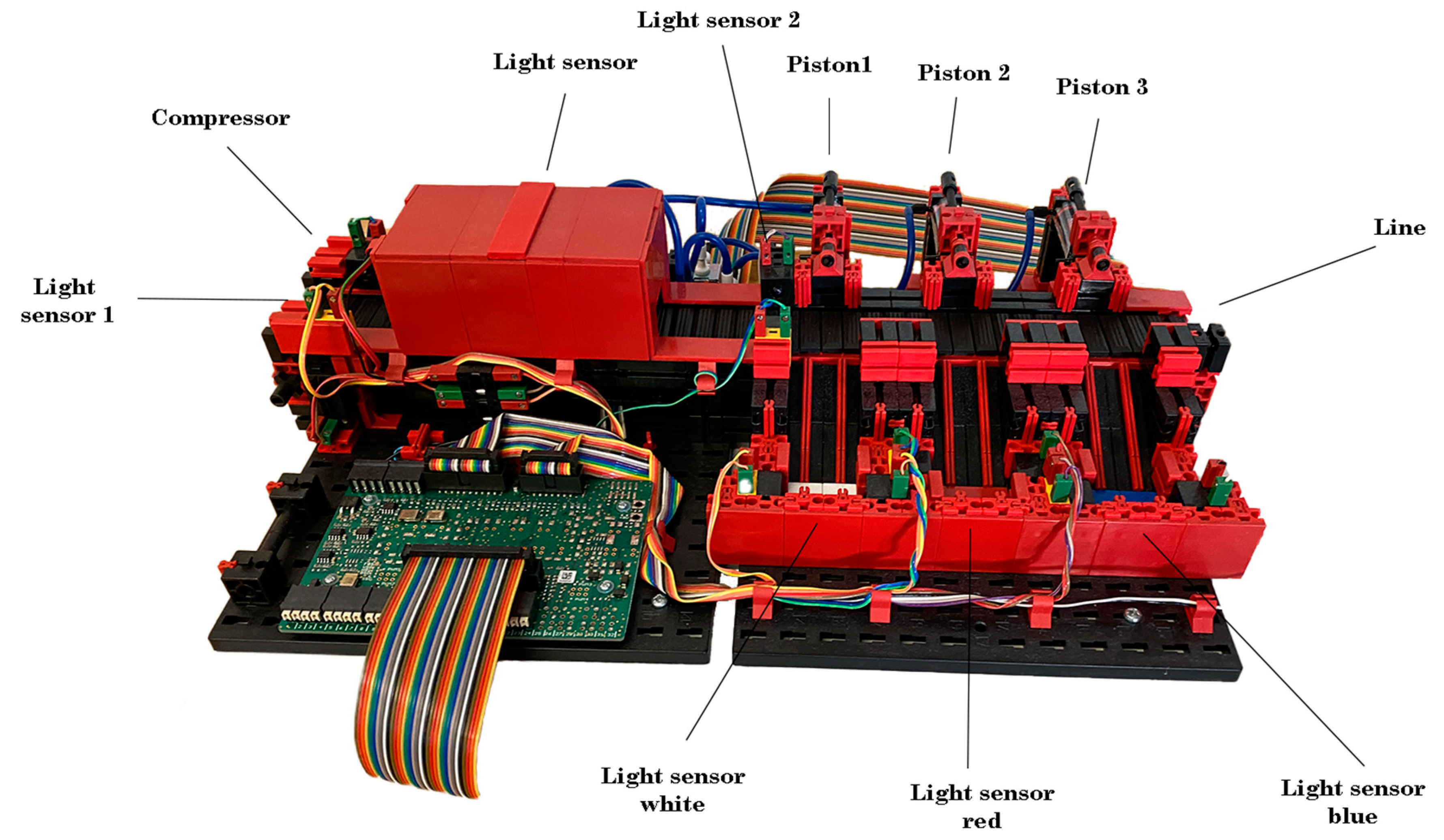
Another laboratory production model is the color detection sorting line model (hereafter referred to as model 2). This system provides product storage based on color recognition. It consists of active members, such as a belt, a compressor, and three pistons. Product color recognition is performed by a color sensor, and information about the product’s position is provided by five light sensors. All listed parts of the laboratory model are shown in
Figure 6.
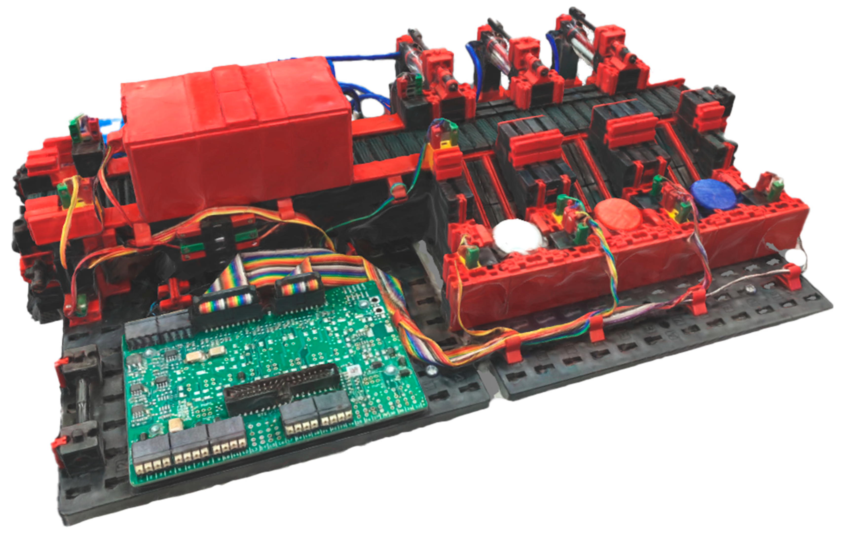
For model 2, we used a powerful PLC device, model S7-1516-3 PN/DP, which provides a higher performance and many more functions than the PLC in the previous case for model 1. The S7-15xx PLC devices themselves do not have inputs and outputs. Therefore, it was necessary to assign input–output modules to the PLC device. In
Figure 6, we can see the control system that we designed and implemented, where the PLC device is connected in combination with four modules and one industrial source. The input–output modules provide us with 32 digital inputs, 32 digital outputs, 8 analog inputs, and 4 analog outputs. The used PLC and output and input modules are placed separately and connected to the controlled production line using wirings.
The last step was the compilation of the algorithm and visualization for model 2. The model is designed for three types of products, red, white, and blue ones. After placing the product on the line, the product moves to the position of the color sensor, where the color of the product is read within 0.5 s.
The algorithm also includes the following functionalities and treatments:
Collision detection for the full storage space—in the case of a full state, it triggers an alarm;
A start function—a treatment for a quick shutdown of the line in the event of an unexpected collision;
Multiple control modes—manual, automatic, and semi-automatic modes;
Counting engine hours for all action members;
Counting sorted products according to the recognized color and the total number of products.
3.3. Cloud Server Development
The next part was to develop and configure the cloud server. In our case, three functional requirements were placed on the cloud server:
We had a choice of several cloud platforms, but, according to the analysis, we decided to use the MS Azure platform [
32]. MS Azure provides many services, from which we have selected the following:
Below, we describe in detail all the services, their design, their configuration, the tools used, and the applications that we have uploaded to the cloud server.
3.3.1. SQL Server + SQL Database
First, it was necessary to create a database in which the data that are provided for remote browsing are stored. From now on, we call these data analytical data. So, we developed an SQL server, called plscwithlove. We stored this server in a data center and together with the server we also created a 2 GB MySQL database. Next, we set up the SQL server as a private server, to which we added the IP addresses of the computer on which the local server was running and the IP address of the server with the backend application. Lastly, we set up security rules for authentication using credentials. We chose the login data according to the general instructions. The password was composed of more than 15 characters and contained numbers, lowercase characters, uppercase characters, and symbols.
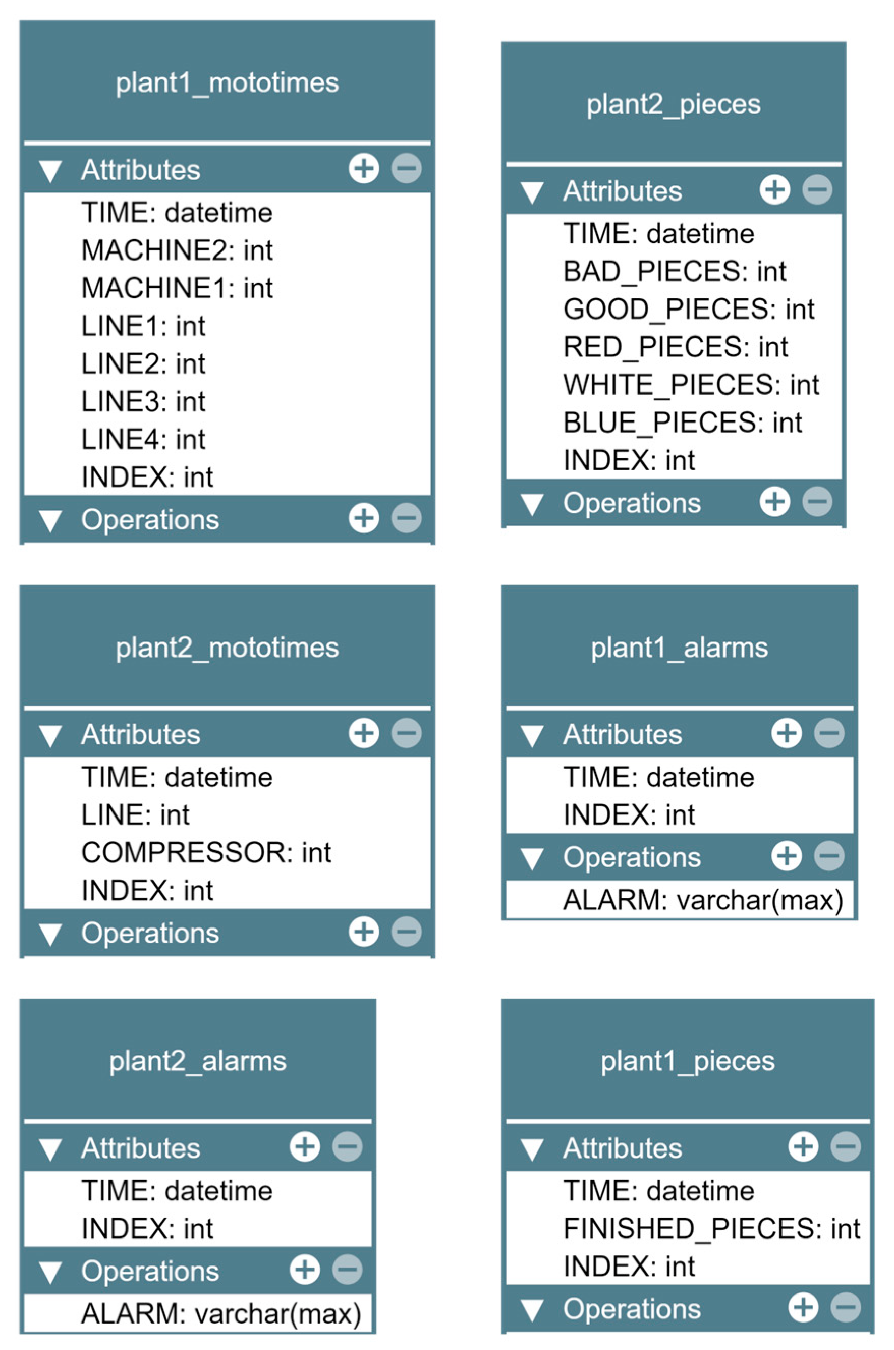
Once the server was configured, we could create the database structure. Each of the production lines contained three groups of analytical data: they were the engine hours, number of products, and alarms. Accordingly, we adapted the structure of the database (
Figure 7). We created six tables in which each row corresponded to one entry. Each of the tables contained a primary key index that was filled in automatically. The other values corresponded to the types of variables that we wrote in the table.
3.3.2. App Service
The next development step was to ensure access to the data using the backend application. Uploading the application was made possible by MS Azure [
33] through the App Service. Here, it was necessary to configure the server environment. We chose the operating system under which the server should work, the Java version of the platform, its location, and which project should be uploaded to it. We chose the location in the data center. Linux, which is compatible with Java applications, was chosen as the operating system, and the Java version of the Java 17 SE platform. As the source of the project, we chose a repository on the Github platform [
34], where we later uploaded the project. In this case, the project is uploaded automatically after the new version of the project is uploaded to the repository.
The backend application had to be created and tested in the initial phase on a local environment. We used the InteliJ tool for development, used the same version of the Java platform as on the server, and created a new project in Springboot framework version 3.0.4 [
35]. First, we connected the application to the MySQL cloud database by implementing the mssql-jdbc library and entering the login credentials. We used the springboot-hibernate library to work with data in the database. With this, we created the basis for our project, and we could further work on creating endpoints for working with data.
The project was based on the REST API architecture in the Springboot framework. For each of the tables, it was necessary to create a model with all attributes. Using the lombok library, we could easily add getter and setter methods for all models using annotations.
Next, we created a repository that directly queried the database. Just like the models, the repositories had to be created separately for each model. Since the repository in the Springboot framework serves as an extension class of the JpaRepository class, there was no need to add new features. All necessary functions were already included in the JpaRepository class. Furthermore, we created services for individual production lines, which provided us with data obtained from repositories for controller classes. In general, the architecture is designed so that the controller configures the path and type that the application queries. Data processing will take place in the service and the repository will provide the data of the given model. In the controller, as already mentioned, we set the endpoint mapping and the http method it responds to. Since data were provided from the backend application, it was a GET-type http method.
We then tested the backend application using the Postman tool, where, after calling the endpoint, the backend application returned data from the database.
3.3.3. Static Web App
As in the previous service, this service also required setting up a server and setting the source from which the frontend application was uploaded. The procedure was the same as in the previous case: we created a new repository on the GitHub platform and connected it to the server. After creating the server, we could start developing the frontend application.
We decided to make the frontend application in the Angular JS framework [
36], version 15.2.3. Currently, a very powerful tool for appearance development is the NgPrime library, which we used in our project to define the appearance of elements on the website.
Before developing the application, it was necessary to build a use case diagram, according to which the application was built. Designed diagram includes two types of users: logged-in and unlogged users. Since the web application is publicly available at the web address
https://wonderful-moss-094cedb03.2.azurestaticapps.net/, e.g., accessed on 6 August 2023, it was also necessary to consider unauthorized access. Therefore, a non-logged-in user can only access the main page and login. In addition to logging in, the application will also include functions such as light/dark mode switching, the display of all lines, and the display of the analytical data of lines in a table and in a graphical interface.
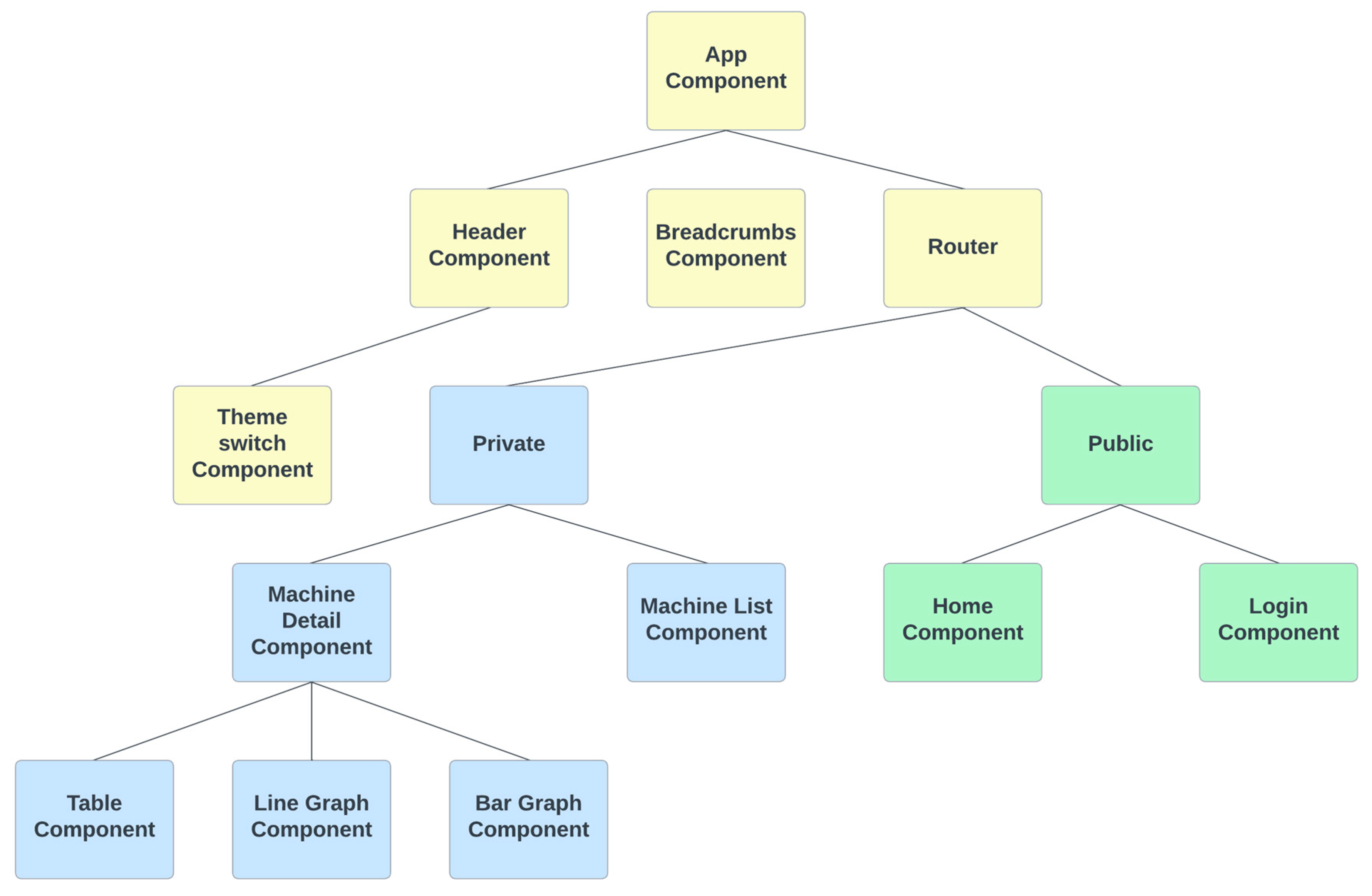
The application was designed to meet current web application standards; be sufficiently clear, intuitive, and minimalist; and avoid unnecessary loading. The designed application can be adapted to mobile devices of different sizes as well as personal computer screens. The application was built using the Angular JS framework, so when the content changes, instead of loading the entire application from the server, only the content that changes is dynamically updated. In the application, we used the angular-router library, which uses the concept of routes to control navigation within the application. Routes are defined as a combination of a path (usually a URL segment) and a component that should be displayed when navigating to the path. We also used the lazy loading technique, which allows Angular modules to be loaded as needed, instead of loading the entire content when the application is launched. This can help improve the initial load time and overall performance of an application, especially in cases where it has many components, services, or other resources. In our application, the initial app-component module is loaded, which contains the main page component and the login component. After the user logs in, the private module with the components of the private part is loaded (see
Figure 8).
As already mentioned, the application can be divided into three groups. They are the basic part of the application, which is found throughout the application, the public part, and the private part. Accordingly, it is possible to divide the components into a diagram. In
Figure 8, we can see a diagram of the components, where the individual parts are distinguished by color. The basic part (yellow color) consists of a header, color mode switch component, navigation (breadcrumbs), and routing. The public part (green color) is accessible to a non-logged-in user, and it includes components such as the home page and login. We present the individual subpages in detail below. The private part (blue color) is accessible only after the user has logged in and includes data visualizations of laboratory production models.
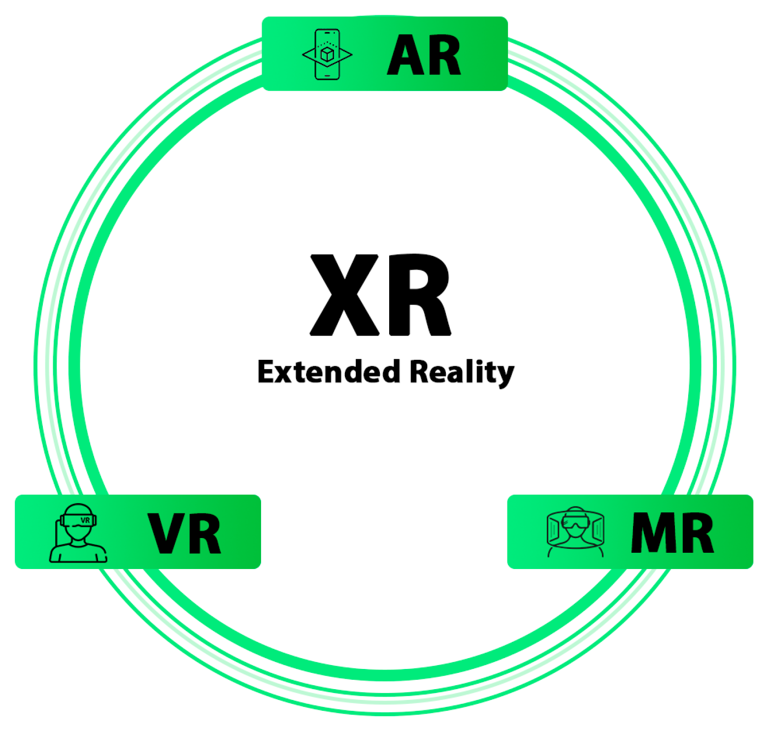
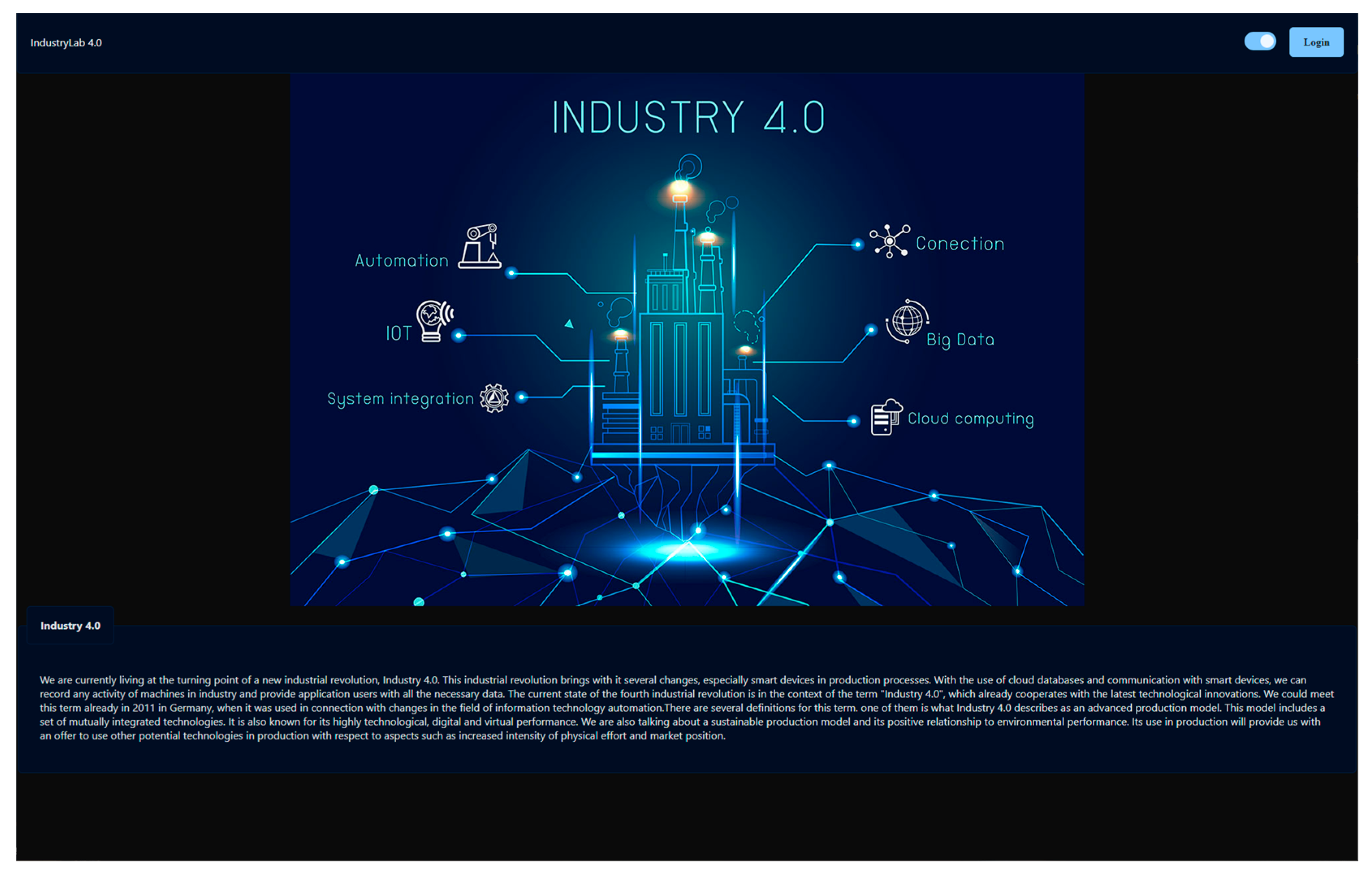
After the initial loading of the web application, we get to the initial page (
Figure 9). There is a header where we can switch the state of the color mode or log in. After clicking on the login button, the application redirects us to the login form. Since the developed platform is based on the Industry 4.0 concept, there is also an image with accompanying text about Industry 4.0 on the opening page.
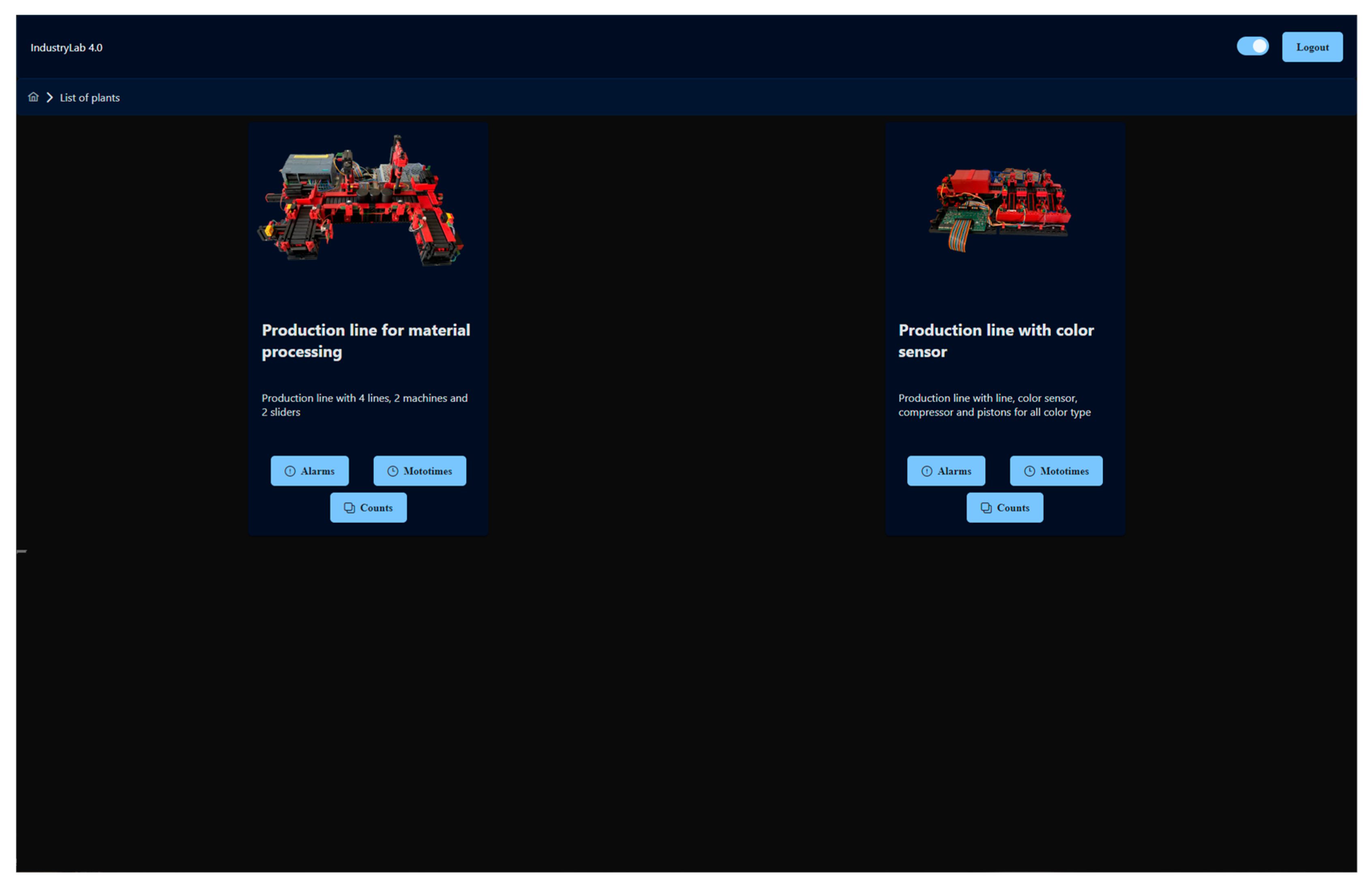
After logging in, the user gets to the list of production lines, which is shown in
Figure 10. This subpage offers the user a quick overview of all the production lines in the system. Each of the lines provides an image of the production line, its name, and a brief description. It also contains buttons that redirect the user to the display of the individual data that the given production line contains.
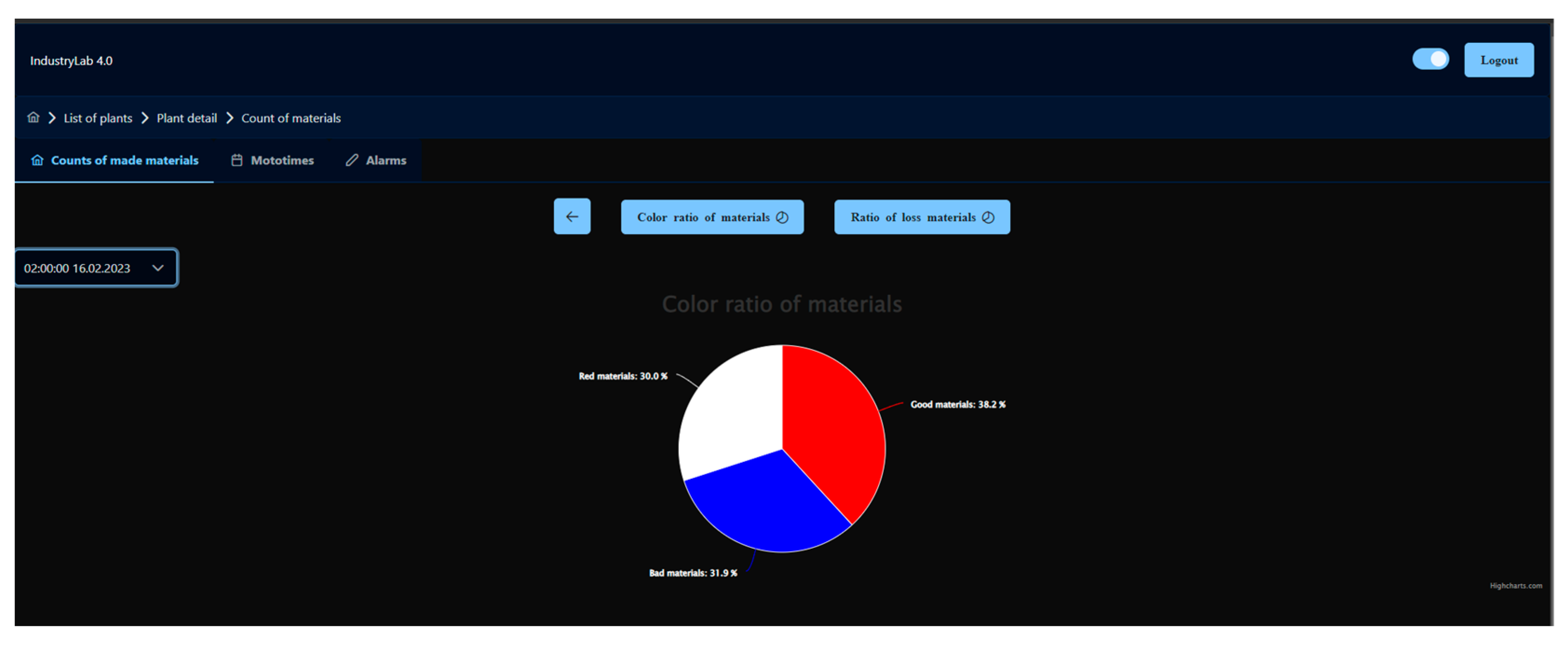
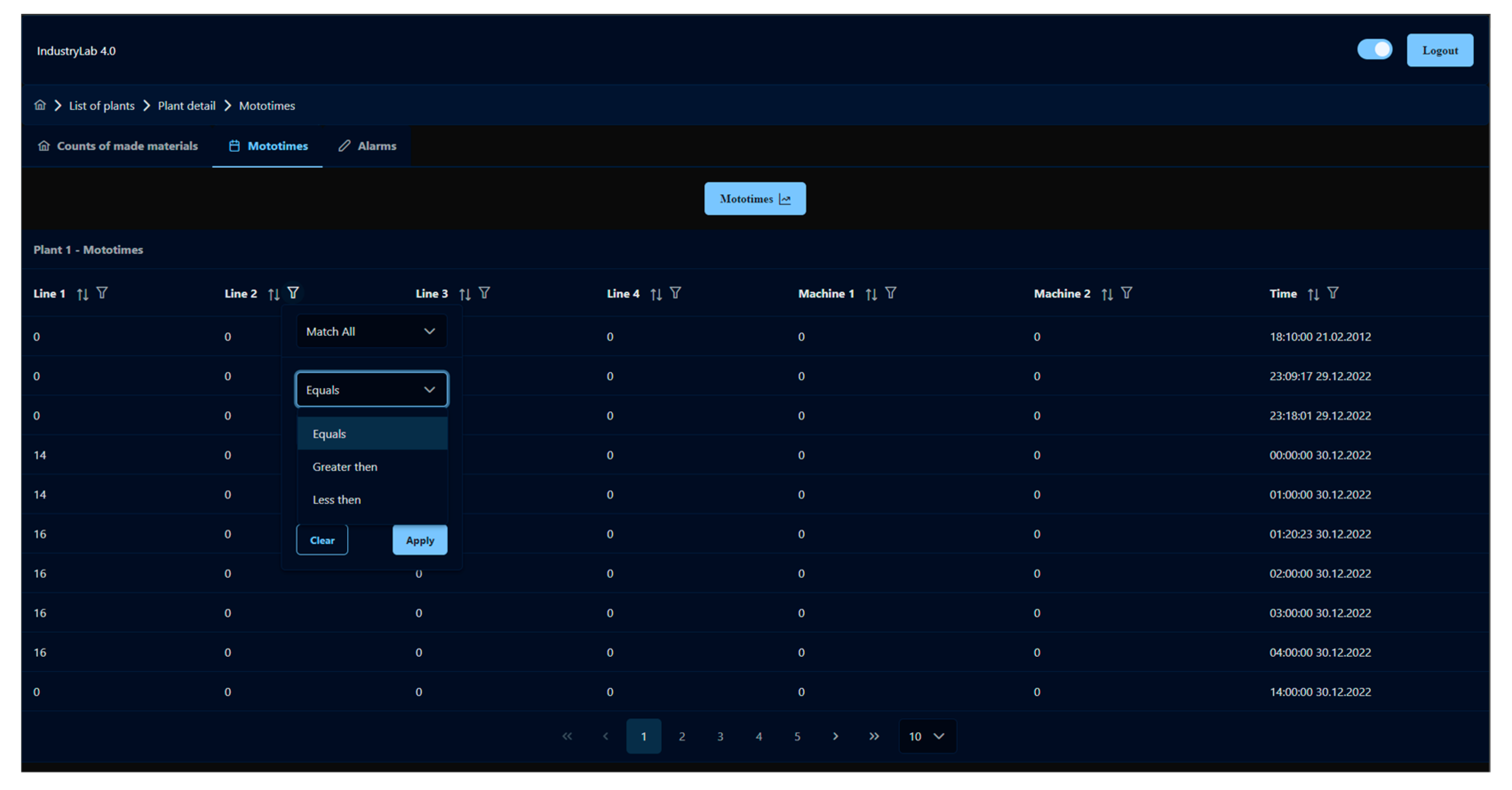
The display of the production line data is represented in tables (
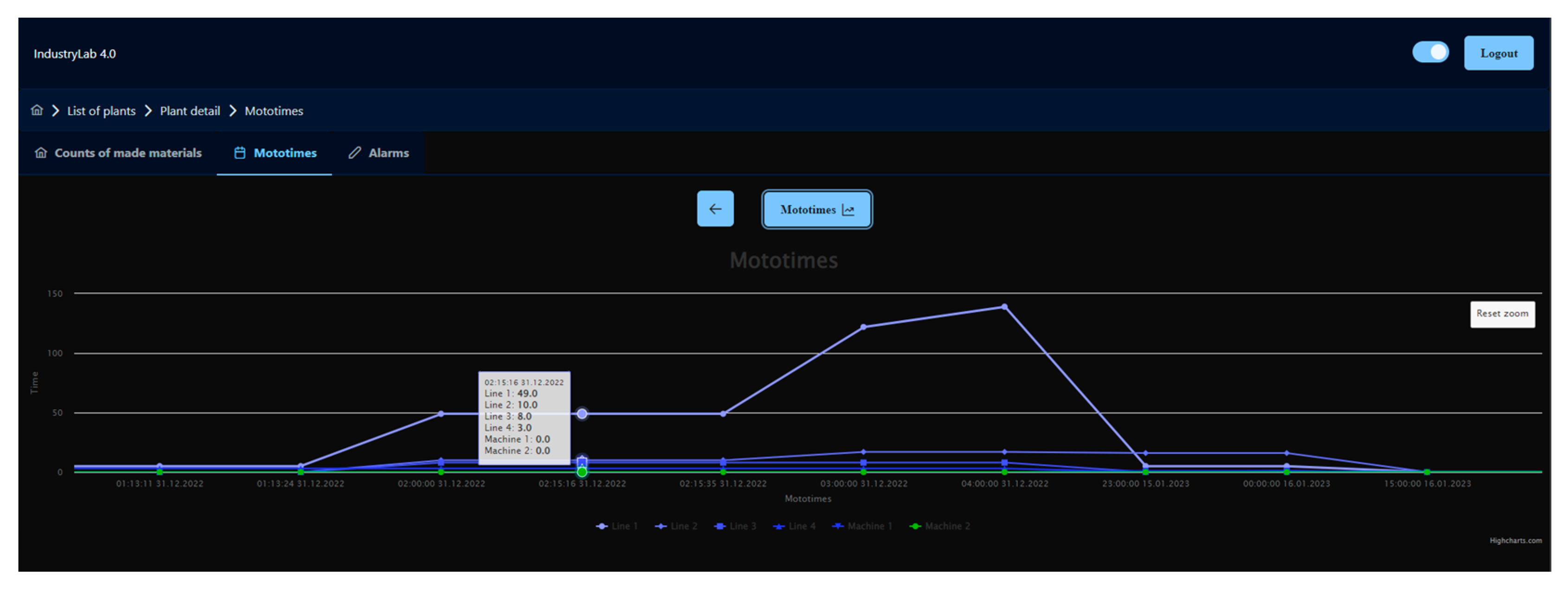
Figure 11). Individual columns can be sorted from smallest to largest (numerically, chronologically, or alphabetically). It is also possible to sort the data according to the entered value. The tables also allow pagination and the option of choosing the number of displayed rows. For each variable from the production line, it is possible to change the data type in the submenu. Each type of data also allows a graphical display of the data after configuration, which is described below. If the data provide a graphical display, a button with the corresponding icon is displayed above the table. The graphical presentation of the data is possible in two ways, a line graph (
Figure 12) and a pie chart (
Figure 13). The line graph allows the display of data in a time plane with the possibility of zooming. The pie chart displays specific data in one record and allows the selection of the given record using the select html element. Every change of data in the graphs is performed with the help of animation.
In practice, it is common for web applications to download data and generate content from them, such as data in a table. But in the HTML code the table expects the exact type of data, so separate components must be made for each type of data. In our case, there is one component for the list of all production lines, one component for the data table, one component for the line chart, and one for the pie chart. How individual components are generated depends on the data we enter into the configuration file. The configuration data for the production line model are compiled in the form of an object. In the entire configuration file, there is an array of multiple data object models from which the cards in the list are generated. The machine key contains the name of the card, the image key contains the path to the image, and the text key contains the accompanying text displayed below the name.
The detail key contains information about whether the given model contains data and what kind. In our case, the models can contain three types of data, alarms, engine hours, and the number of products. Therefore, the detail contains the keys’ alarms, times, and counts. Each of the details contains the same data, which are also in the form of an object. In this object, the show key determines whether the model contains these data. If it does not contain them, the given button is not displayed in the model tab and it is not possible to click on the given data in the model detail submenu. The title key contains the name of the table, and the path key contains the path to the endpoint from which the data are requested. In the header key, all the columns that are displayed in the table are in the field, and each of the columns contains settings, such as its name, whether it can be sorted, and what type of data it contains. The data type determines what filtering would be applied to that column. Furthermore, the data key contains all the data that should be displayed in the table. The individual data contain their name in the data that are obtained from the backend and in what way they should be transformed. In our case, we only transform dates to the dd.mm.yyyy format.
The last key is the graphs key, which determines how many and what kind of graphs for a given type of data are provided. The configuration data for the graphs are in the format of an array, according to which the graph buttons above the table are generated. Individual graphs represent objects in which the type key determines whether it is a line graph or a pie graph. The buttonText key contains the text displayed in the button above the table. The show key determines whether the graph will be displayed by default (in priority over the table) when displaying data. The unit key specifies the name of the x-axis and y-axis in the string format “axisX~axisY”. The moreTimes key determines whether the select html element will be displayed with all of the time data. The data key determines which data will be displayed on the graph, and in the color key we can choose our own colors for individual data.
If we leave only an empty field in the color key, the colors will be determined by default. If we also leave the graphs key as an empty field, then the data will not contain any graphic representation of the data.
3.4. Development of a Mixed Reality Application
The important part of the smart platform development was the creation of an application for mixed reality, which we implemented in the environment of the Unity game engine. We worked specifically in version 2020.3.33f1, which is verified for compatibility with the MRTK software 2.8 development toolkit. This part is one of the key paper contributions, as it enables the detection of a real production model in mixed reality and contains an algorithm for a generic rendering of the visualization of individual production models. As part of the development, it was necessary to implement the following libraries and settings into the Unity application:
Set up an application for MRTK development;
Implement the MQTT library for communication with the local server;
Implement the Vuforia library for object recognition;
Create an algorithm for rendering the user interface.
Next, we describe the procedure for individual implementations of functionalities in the project.
3.4.1. MRTK
It was necessary to set the project up to be compatible for work with MRTK. Since the MRTK package is not in the package manager, the implementation had to be performed using the MS Mixed Reality Feature Tool, an external application. Using this application, we were able to import the MRTK package into the Unity project.
3.4.2. MQTT Communication
We used the M2MqttUnity library to implement MQTT communication in the Unity project. It provided us with basic functions, such as connecting and disconnecting to the MQTT broker, receiving data from the given session, and sending values to the MQTT sessions, which we specified. We laid the foundations of our communication algorithm on these functions.
The ConnectToMQTTServer function ensured the connection to the MQTT broker. The input data were a string in the format ipAdresa~port. Based on the received data, the function connected the application to the MQTT broker. The default value of the input string was 192.168.50.60~1883, which ensured that the function was called without entering data. Also, the algorithm contained a function for disconnecting communication, which was provided by the DisconnectFromMQTTServer function. This function also provided disconnection from all sessions that were active at the given time.
The function SendDataToMQTTServerByValue ensured the sending of data. In this case, the input variable was of the GameObject type. Each button that interacted with one of the variables from the PLC device contained all the necessary data for communication. This also enabled the simple implementation of our algorithm, where the data it contains was not specified in advance. From the name of the object, the type of variable was found out, and it was taken from the global variable, which contained all the data from the PLC device. Subsequently, the data were sent to the MQTT broker.
The SubscribeTopics function provided us with a connection to the MQTT session. Functions like StartSubscribePlant and GetJSONPlant were built on top of this function. The StartSubscribePlant function allowed to connect to one of the models. This includes disconnecting from all sessions, clearing the current global variable, connecting to the systemX_initializer, the systemX_reader session, and requesting initialization data. The GetJSONPlant function, in turn, connects to the systemX_json session and requests user interface data for the given system.
Another important function was the OnMessageArrivedHandler. This decided the treatment of the data that the Unity application received from the MQTT broker. In this case, whether the data were user interface data or actual data from production models was recognized. We present both cases of data processing in detail below.
In the communication structure, the local server was the data intermediary between the PLC device and the Unity application. The local server therefore did not keep information about the state of all data, but these states had to be stored in the Unity application. However, since the Unity application is not specified for one type of production model, it was necessary to provide a dynamic variable with different types of data and different keys. Therefore, an important part of the proposed MQTT implementation is also the method of data storage in the Unity application.
The data storage resides in the GlobalVariables static class we created. This class contained the variable MQTT_data in the form of a dictionary, which was based on defining a key in a string format and also data in a string format. It was necessary to store the data in one form, as Unity has a very difficult time working with dynamic variables. The class also contained functions for handling global data. They were functions such as the getter, the setter, dictionary emptying, data format checking functions, or data format converting functions.
The getter and setter were functions based on returning or storing data based on a key. In the case of the setter, if the key was not found in the dictionary, a new key was created with the value we wanted to write. In the case of the getter, if the given key was not found in the dictionary, a null value was returned.
When initializing the new model of the production line, the data were filled with all the variables that the given PLC device contained, and when the data changed it simply updated the data to the current value. During MQTT communication, all data were received in a string format and therefore it was necessary to first convert them to the JSON format, from which the name of the variable and its value were then obtained. The global data could not be updated from the Unity application; every data change was sent to the PLC device, and, based on the change in the given variable in the PLC device, its current value was accepted. In this way, we ensured the reliable display of the current values of all variables from the PLC device, and it was impossible for the application to display the wrong value.
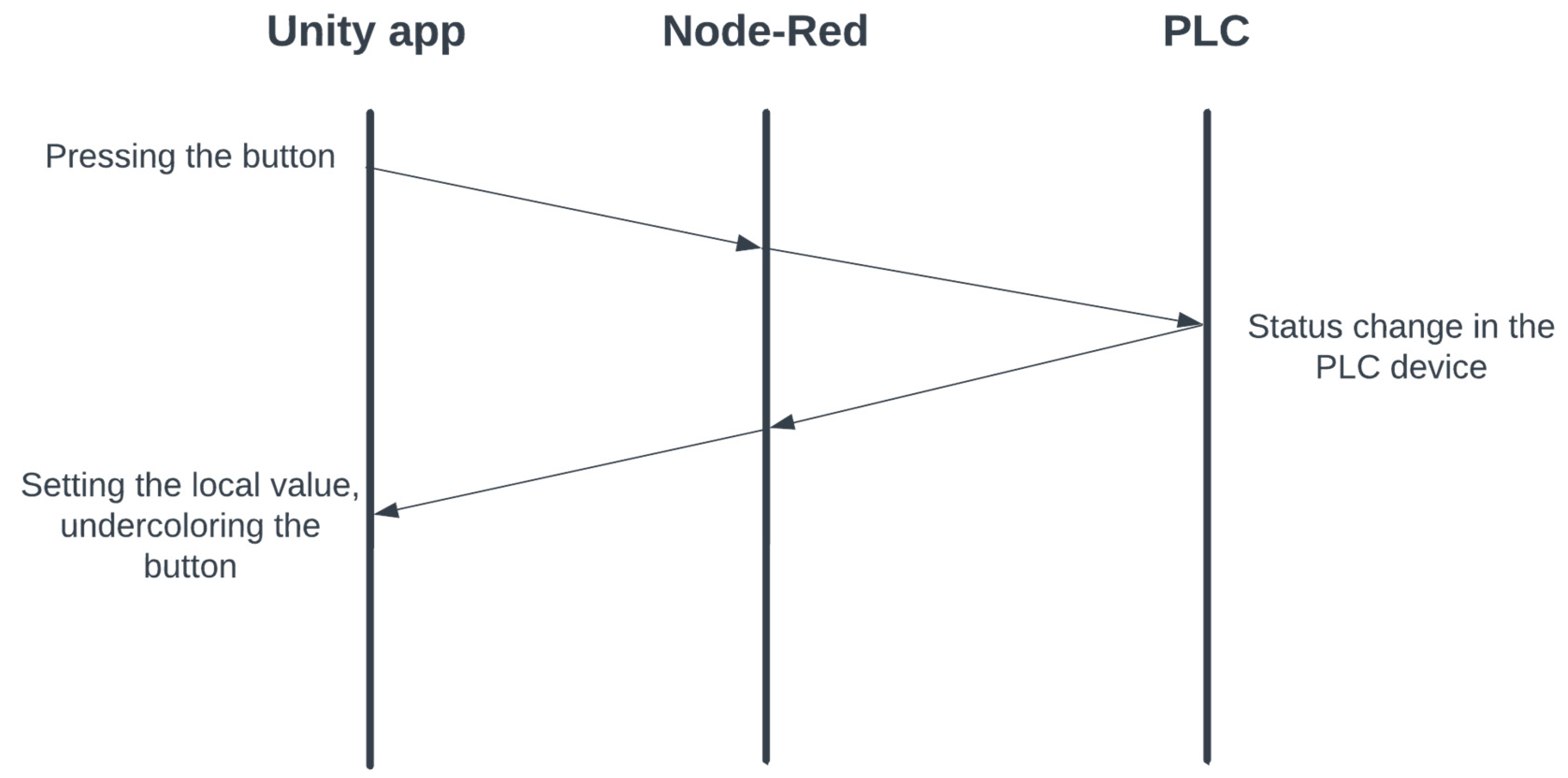
An example of communication can be seen in
Figure 14. When the button is pressed, we send the value of the given variable using MQTT communication, which sets it in the PLC device. The local server records the change of the given variable and then sends it using MQTT communication to the Unity application, where the change in the value of the variable is stored in (from the point of view of the application) a global variable.
3.4.3. Vuforia
Vuforia [
37] is an augmented reality (AR) software platform that enables developers to integrate digital elements into the physical world using mobile devices. The implementation of Vuforia in the Unity project allowed us to recognize 3D objects and track them in real time. But this was preceded by the creation of 3D models of production lines, based on which Vuforia was able to recognize a real object.
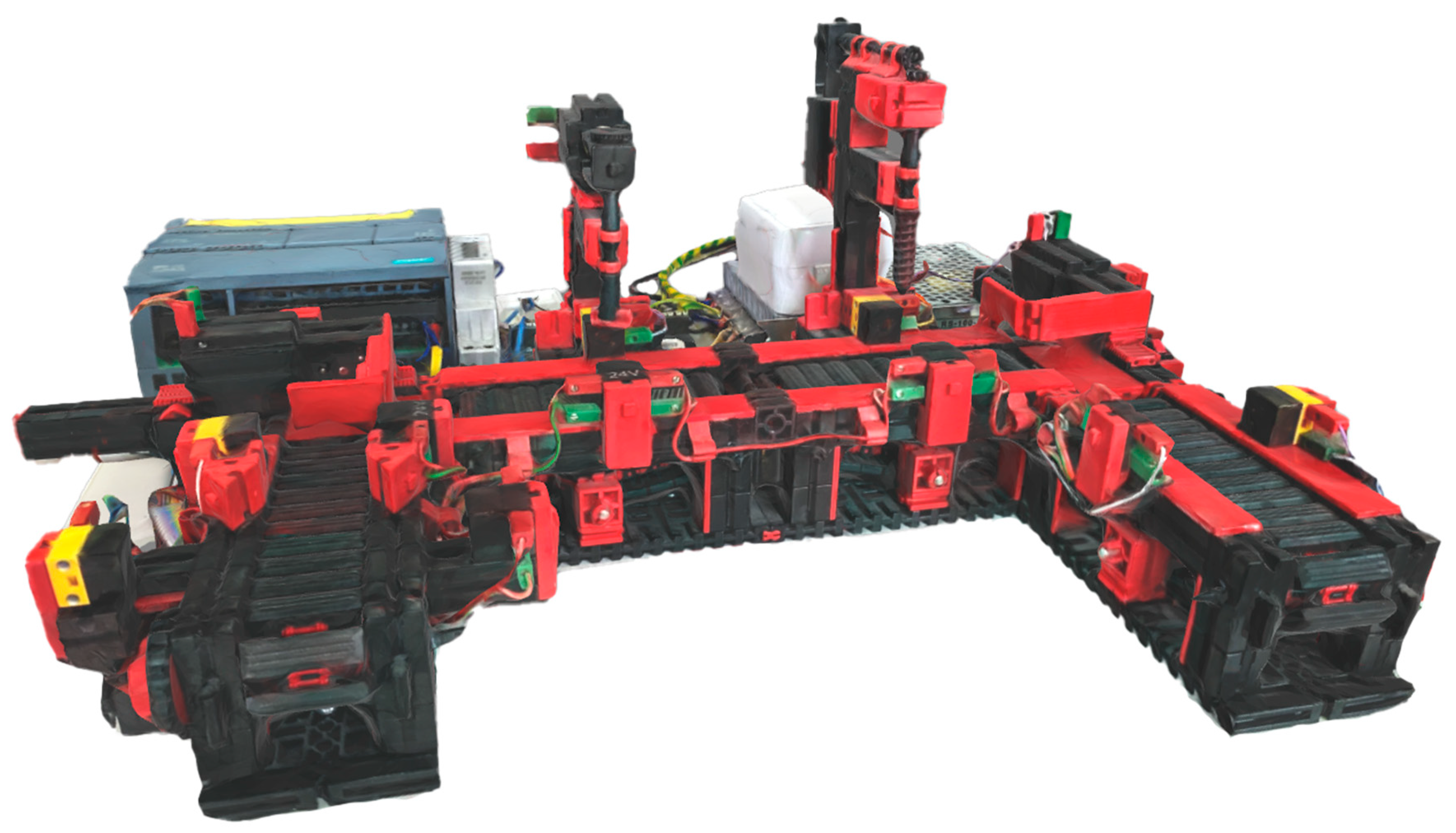
We tested several applications for creating 3D objects of production lines, such as Polycam, Scandy Pro, Metascan, Qlone, and MafiScan. Polycam was the most effective, providing us with the most authentic 3D models at no cost, with object size data that could be exported in common 3D model file types, e.g., in an .obj or .fbx format.
Using the Polycam application, we scanned 3D objects using a mobile device. In our case, it was an iOS mobile device, the iPhone 11 Pro Max. The device had a sufficiently high-quality camera, with which we captured more than 100 photos of the laboratory model of the production line. These photos were used by the application to create a 3D model of the corresponding production line and export it to an .fbx file. In this way, we created 3D models of the production lines. In
Figure 15 and
Figure 16, we can see scanned 3D models created using the Polycam application.
To detect real world objects, it was necessary to train the recognition of real models based on the obtained 3D models. This was enabled by the Vuforia Model Target Generator application. Based on the obtained 3D models, we created the SustavyPro database, which contained the data of the 3D models.
It was necessary to import the Vuforia Engine AR library into the Unity project. We implemented the trained database into the Unity project and created all the necessary objects for recognizing real objects. Here, all Vuforia objects had to be put into an empty object called VuforiaContent. If we skipped this step, the Vuforia library would not record objects at all. Objects System1 and System2 represent 3D objects, based on which real objects are recognized. Both objects required a connection to the database and the target model in the database. After connecting the target model, the dimensions of the object were automatically delivered.
Another necessary configuration was to set what should happen when objects are recognized and lost. We use the RecognitionObjects object for this, which provides functions that are performed in these events. When the object is recognized, the Unity project connects to all MQTT sessions, requests the local server for the JSON UI, and, after rendering the user environment, requests all the initialization data of the PLC device of the given system. When the object is lost, it is disconnected from all MQTT sessions and the currently generated user environment is deleted from the scene.
3.4.4. User Interface Rendering Algorithm
As already mentioned, the application renders the user interface of individual production lines based on the data defined by us—the JSON UI. The data reside in files on a local server where they can be changed at any time without the need to build a new version of the Unity application.
When receiving data from the local server, the MQTT session the data were received from is monitored. If the data were received from a session that carries a JSON string, the data will be treated according to the user interface rendering algorithm. This algorithm consists of the following steps:
Reformatting data from a string format to a JSON format;
Removing the previous user environment if it exists in the scene;
The rendering of a new user environment;
Connections to all MQTT sessions of the recognized production line;
A request for initialization data of the current production line.
In the C# programming language, when formatting from a string we are expected to know in advance what data format the string will give us. In our case, we expect data in the form of an object that carries information about the name of the production model and its number. Based on the name of the model, the algorithm determines to which object in the scene it will render all the objects. Thus, if we accept the name PLC1, the data will be rendered into a 3D object named MenuPLC1. Each of the 3D models of production lines contains such a menu object, thanks to which we ensure that the user environment of the production line will always be located at the coordinates of the recognized production line. The production line number, in turn, determines which MQTT sessions the Unity application will connect to.
Furthermore, the object contains the field content, which represents the content of all the objects located in the user environment, for example, background objects that contain nested objects, such as texts, buttons, squares, or circles.
The background object contains information: the name of the 3D object, the background color, the visibility of the 3D object, the position and size of the 3D object, and the nested 3D object’s content. We can set the background color to red, green, yellow, blue, gold, black, or white. The background color is represented as a renderer component, and the color spectrum is determined using the spectrum map. Every color that can be set on a 3D object was created in Photoshop. Since the user environment can contain several panels, the visibility of the 3D object determines which one will be active during rendering. When switching between panels, the currently displayed panel is deactivated and the panel to which we want to switch is activated. Nested 3D objects represent all objects that are displayed on the given panel. We list them below.
The key of the position object carries the data that each of the objects in the JSON UI representing the 3D object contains. It contains posY, posX, and posZ data, which are represented in a float format and determine the position of the 3D object depending on its parent 3D object. It also contains scaleX, scaleY, and scaleZ data, which determine the size in individual axes.
The key of the content object contains the array of nested objects that are located on the given panel. Depending on the type of 3D object, the data object can contain different data. Each data object representing a nested object contains data, such as the name, tag, gameObjectType, and position. Depending on the type specified by the gameObjectType key, the data object may additionally contain buttonProperties (in the case of a button), textProperties (in the case of text), or squadProperties (in the case of a circle and square).
Common data determine the basic properties of 3D objects. The name key represents the name of the 3D object, and the tag key specifies the tag to be assigned to the 3D object. According to the tag of the 3D object, which MQTT session the data will be sent to is determined. The gameObjectType key specifies what type of 3D object it is: in the case of a button, it contains the value button; in the case of text, it contains the value text; in the case of a square, it contains the value squad; and in the case of a circle, it contains the circle. The position key, as already mentioned, determines the position and dimension of the 3D object.
If it is a 3D text object data, it is supplemented with the text value (text), font size (fontSize), text color (textColor), text style (fontStyle), vertical alignment (verticalAlign), and horizontal alignment (horizontalAlign). In the case of the text type, the values can be normal, bold, or normal. The color of the text can be defined using the values black, white, red, blue, yellow, or green. The text can be aligned in the vertical plane using the values center, top, and bottom and in the horizontal plane using the values left, right, center, or flush. The flush value aligns the text from one edge to the other.
The 3D objects squad and circle are the simplest objects in the algorithm, and they only contain the color value, with which we can change the background color of the object. A circle, unlike a squad 3D object, is rendered with a 50% radius.
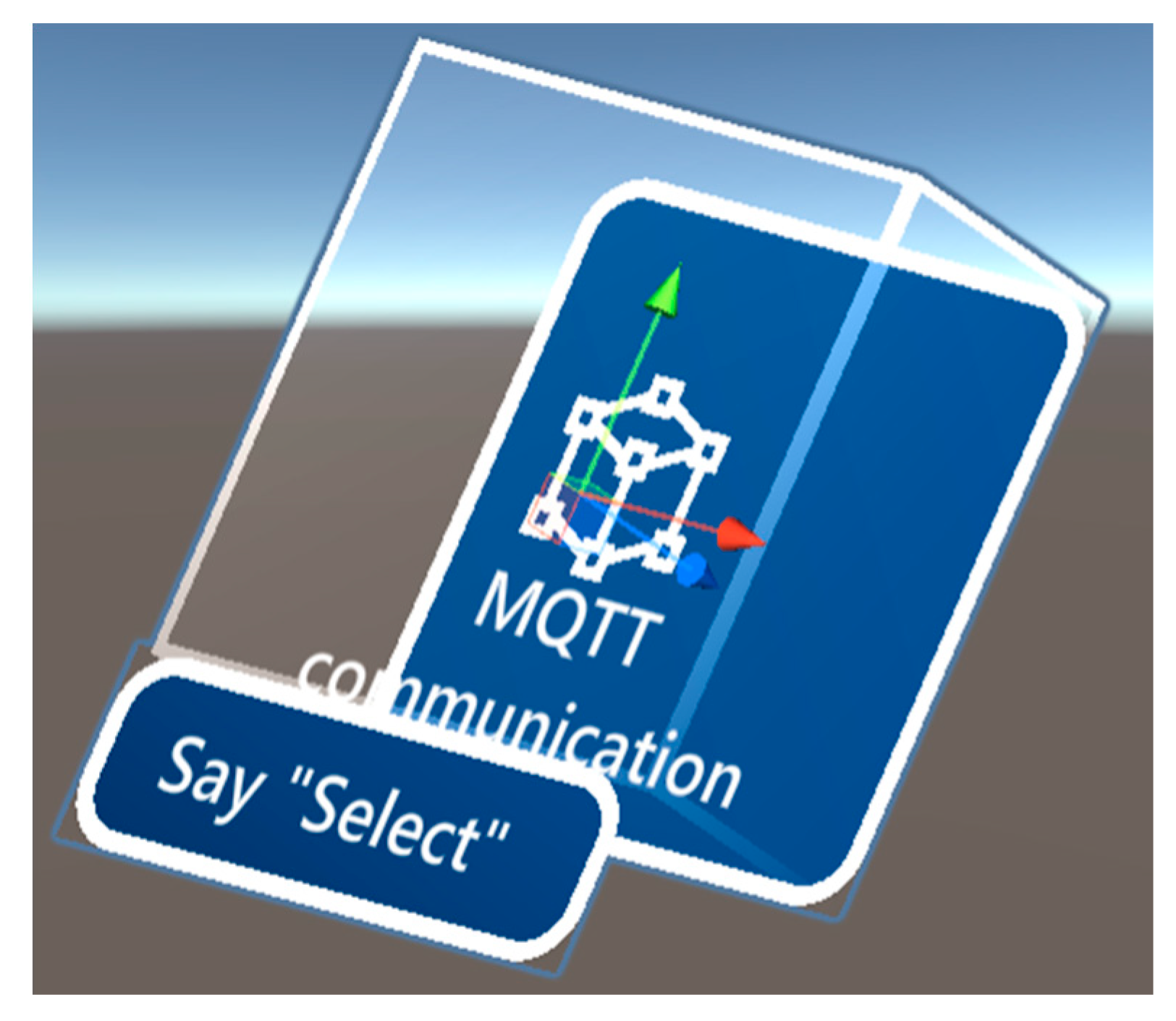
Button-type 3D objects are the most complex objects in our algorithm. In addition, the data contain the text that is displayed on the button and in the text label, to which the application reacts when controlled by the speech label. The setting of the icon of the button is enabled by the icon key, and the color of the button is set by the color key (with the same values as the background). The clickable key carries a Boolean value that specifies whether the button is clickable and a list of functions that will be performed when the button is pressed. If the button control is not enabled, the function list is ignored. Enabling button control determines whether the button will also include a visualization of the button outline in a 3D environment (
Figure 17).
Individual functions contain data, such as the function name (functionName), variable value, and variable type (variableType).
There are several functions to choose from:
SendDataToMQTTServerByValue—sending data to the PLC device with value negation;
SendDataToMQTTServer—fixed sending of data to the PLC device with a static value;
HandleVisibility—switching the active panel;
HandleVisibilityByControl—switching the active panel based on a variable;
HandleVisibilityByControlWithOtherValue—the same function as the previous one, enriched by sending data to the PLC device.
Since some 3D objects, such as a button, contain multiple nested 3D objects, it would be too complicated to create new 3D objects in a script. Therefore, we created predefined 3D objects, called prefabs, in Unity. Based on the received data, we used specific prefab objects for buttons, texts, backgrounds, or squares/circles and adjusted their configuration according to the object type.
3.4.5. Appearance of the Application
Since the application was developed for the MS HoloLens 2 device, the appearance of the application was designed according to the MRTK design. The components from the MRTK templates library were used and modified according to our needs.
The application contains a main menu with the option of activating and deactivating communication with the MQTT broker, displaying the active production line, and debugging buttons for activating individual production lines. Since it is a mixed reality application, it was not possible to use common practices, like web or mobile applications. The menu is therefore realized by following the user with the possibility of opening and closing, as it occupies a large area when open. The menu is animated upon interaction.
Each of the lines provides multiple panels, and when a production line is recognized an initial panel is displayed with the option of redirecting to all panels that the production lines contain. Redirection is performed by pressing the button. Each panel in this section is generated from the JSON UI.
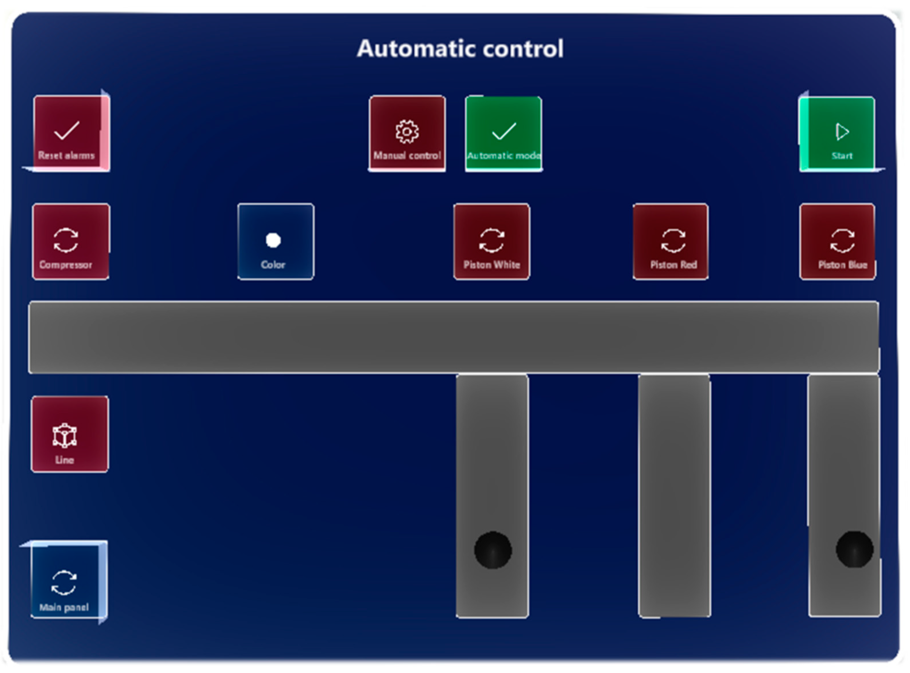
For each of the control modes of the laboratory production models, a panel was designed according to
Section 3.1. When switching control modes, the panels corresponding to the activated control mode are also switched automatically. In
Figure 18 and
Figure 19, we can see panels of automatic modes at both production lines. In the manual mode, we can see the same layout of objects, with the difference that the buttons respond to pressing; in the automatic mode, the buttons are blocked.
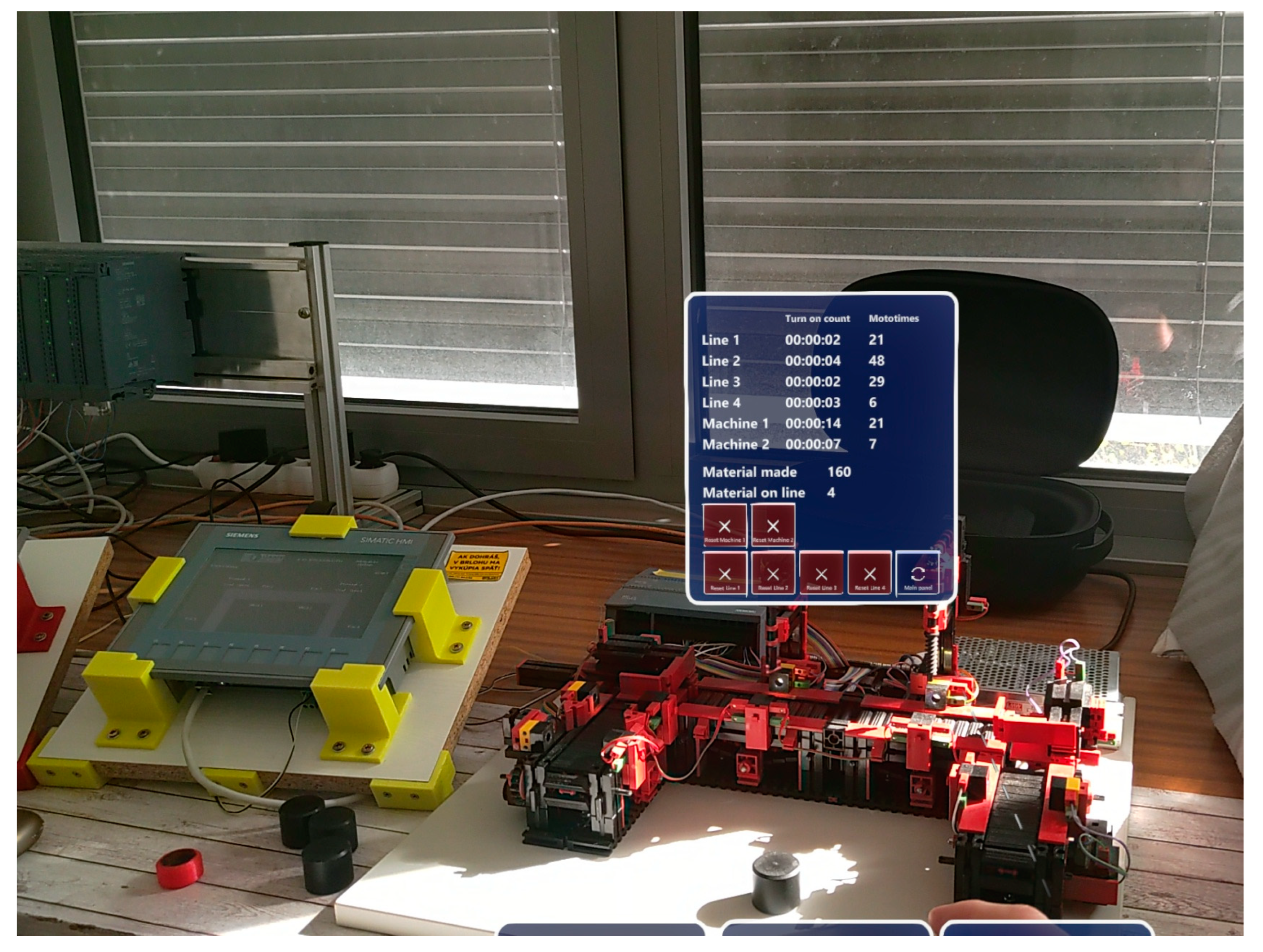
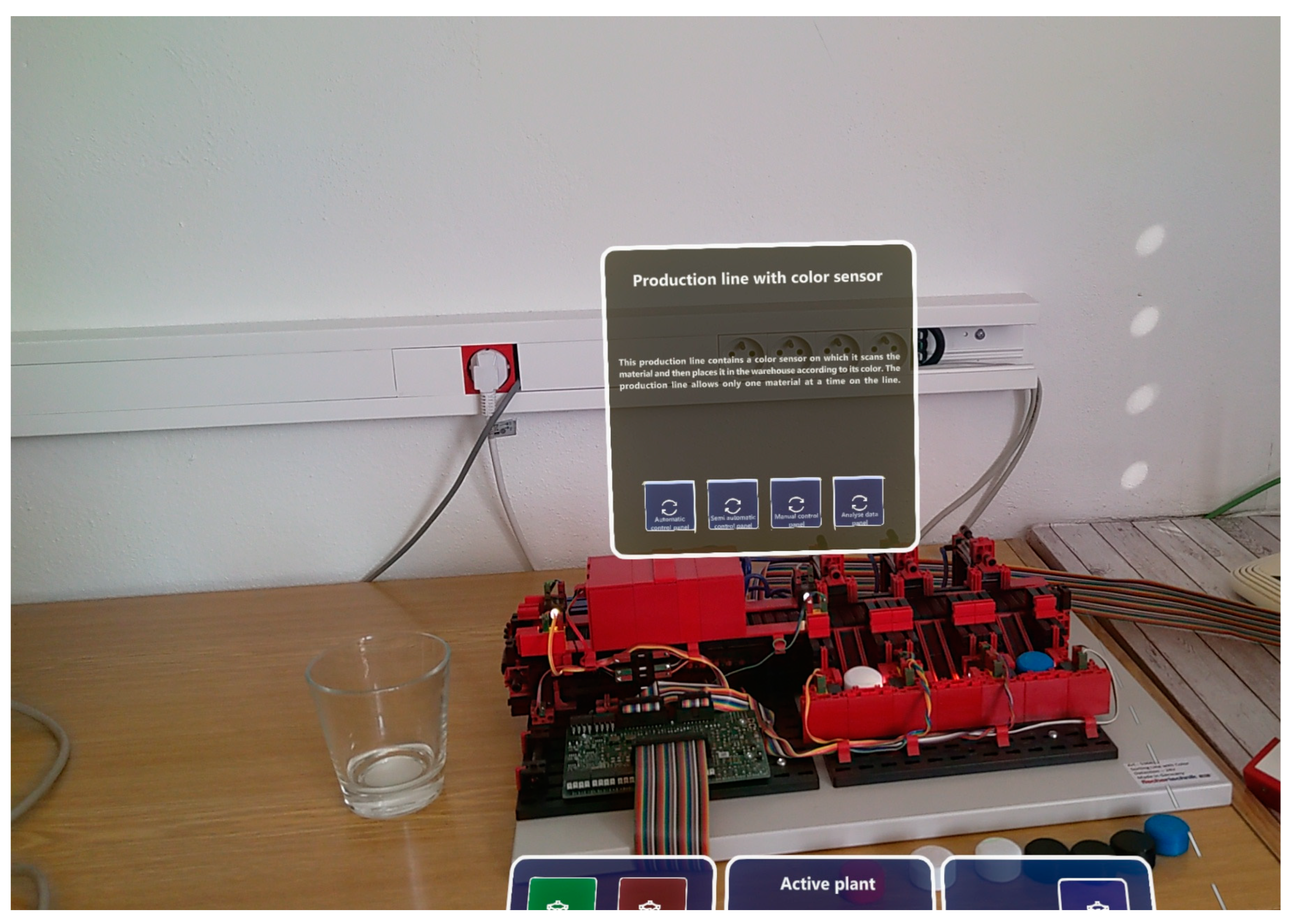
Once the line is recognized in the real world, the panels appear above the production line and hold that position throughout. With the loss of the detected production line, the panels are erased from the virtual reality scene. As the user moves, the panels tilt behind the user, thus ensuring a good viewing angle from any position of the user. Virtual panels placed above real production lines can be seen in
Figure 20 and
Figure 21.


