Faster R-CNN-LSTM Construction Site Unsafe Behavior Recognition Model

Abstract

Aiming at the problem of insufficient accuracy caused by the insufficient mining of spatiotemporal features in the process of unsafe behavior and danger identification of construction personnel, the traditional two-stream convolution model is improved, and a two-stream convolution dangerous behavior recognition model based on Faster R-CNN-LSTM is proposed. In this model, the Faster R-CNN network is connected in parallel with the LSTM network. The Faster R-CNN network is used as the spatial flow, and the human spatial motion posture is divided into static and dynamic features to extract the anchor point features, respectively. The fusion of the two is used as the output of the spatial flow. An improved sliding long-term and short-term memory network is used in the time flow to increase the extraction ability of the time series features of the construction personnel. Finally, the two branches are fused in time and space to classify and identify whether the construction personnel wear safety helmets. The results show that the MAP of the improved Faster R-CNN-LSTM network framework is increased by 15%. The original CNN-LSTM network framework detected four targets, but there was one misdetection, with an accuracy of 91.48%. The improved frame detection accuracy reaches 99.99%, and there is no error detection. The proposed method is superior to the pre-improvement and other methods that can effectively identify the unsafe behavior of construction workers on construction sites and also has a good distinction effect on fuzzy actions.

1. Introduction

Human unsafe behavior recognition stands at the crossroads of safety management and artificial intelligence applications, playing an indispensable role in preempting criminal activities and fortifying accident responses [1,2,3]. This state-of-the-art technology hinges on computer-assisted video analyses, pinpointing and classifying specific human actions. Yet, the effectiveness of these systems is, more often than not, impeded by challenges like occlusions, motion perspective shifts, and intricate backgrounds, all of which complicate exhaustive information extraction [4,5,6].

The construction industry, infamous for its high incidence of safety mishaps attributed to human behaviors, presents a pertinent case study [7,8,9]. Traditional safety oversight, largely predicated on managerial surveillance, exhibits glaring inefficiencies, exacerbated by transient personnel, rapidly evolving environments, and convoluted production dynamics [10]. Even with the exponential growth of data-driven insights, hurdles such as integration bottlenecks and elevated overheads persist, necessitating an innovative shift in construction safety paradigms.

Amidst this backdrop, intertwining safety management with computational methodologies is emerging as a promising research direction. The recent renaissance in deep learning equips us with sophisticated object detection frameworks—algorithms like R-CNN, Fast R-CNN, and YOLO being prime examples [11,12]. These pioneering technologies herald a transformative era in safety management, streamlining data acquisition, processing, and dissemination.

The scholarly community has made remarkable headway in worker safety helmet detection, leveraging cutting-edge algorithms. Hu et al. [13] laid the groundwork, birthing the inaugural algorithm tailored for automatic worker safety helmet identification. Subsequent trailblazers like Fang et al. [14] and Zhang Mingyuan et al. [15] further refined detection accuracy. Delving into nuances, Wu Dongmei et al. [16] and Wang [17] extended detection capabilities, differentiating helmet nuances and optimizing detection metrics. In the realm of ear print recognition, Aiadi et al. [18] introduced MDFNet, a lightweight unsupervised network known for its efficiency. Utilizing gradient magnitude, direction, and data-driven filters, MDFNet outperformed many existing methods, showing high recognition rates and robustness against occlusions on three public datasets. Despite such advancements, glaring gaps persist. Contemporary detection methodologies often neglect intricate spatiotemporal dynamics ingrained in human motions. Human action recognition is inherently nuanced, necessitating the discernment of both distinct action types and subtle variations within identical actions. The predominant models, particularly spatiotemporal two-stream convolution, falter when faced with intricate or ambiguous human behaviors.

While these strides in helmet detection technology are commendable, the broader domain of human behavior detection still grapples with challenges. Most existing methodologies tend to overlook the complex spatiotemporal dynamics inherent to human movements. The intricacies of human action recognition are profound, given its nature of interclass recognition; not only do we have to categorize distinct types of actions, but there is also the nuance of identifying subtle variations within the same action, often influenced by its amplitude or intensity. Conventional models, especially spatiotemporal two-stream convolution, find themselves outpaced in scenarios demanding the recognition of complex or ambiguous human actions. Recognizing these gaps, this paper ventures to introduce an optimized two-stream convolution model, meticulously crafted for pinpointing unsafe behavior.

2. Method

2.1. Convolutional Neural Networks

Convolutional Neural Networks (CNNs) have emerged as a cornerstone in the realm of deep learning [19,20,21]. Their prowess lies in processing data with a grid-like structure. A quintessential example of this would be images, where data can be visualized as a two-dimensional grid made up of pixels. One of the core processes in a CNN is the convolution operation, designed to automatically extract a range of features from the input data [22]. The design of a CNN as a spatial stream is geared towards capturing spatial features within images, especially those pertinent to human dynamics and postures. The localized nature of convolutional operations allows for the detection of localized features in images, such as edges, textures, and shapes, which are instrumental in recognizing human postures. Through pooling operations, CNNs exhibit spatial invariance, ensuring that humans can be detected regardless of their position in an image. Multiple convolutional and pooling layers in CNNs facilitate multilevel feature extraction, ranging from rudimentary edges and textures to intricate human body parts and postures.

Convolutional Neural Networks (CNNs) primarily comprise two processing stages: the feature learning phase and the classification phase. The feature learning phase is realized through a combination of convolutional and pooling layers. This phase is dedicated to extracting the most salient features from training examples. Subsequently, these extracted features are fed into fully connected layers. The final layer of a deep neural network typically consists of a fully connected layer combined with a Softmax classification network, producing a classifier with a number of classes equivalent to the requirements of the project.

(1) This operation involves moving through the input data using a convolution kernel, based on a predefined step size, known as the “Stride”. Each of these movements entails a convolution operation. To grasp this concept in a more mathematical sense, consider the following formula: In this paper, the VGG 16 model is selected in the spatial flow. The model uses a 16-layer deep network, including 13 convolutional layers and 3 fully connected layers. The convolution kernel is 3 × 3, and the step size is 1.

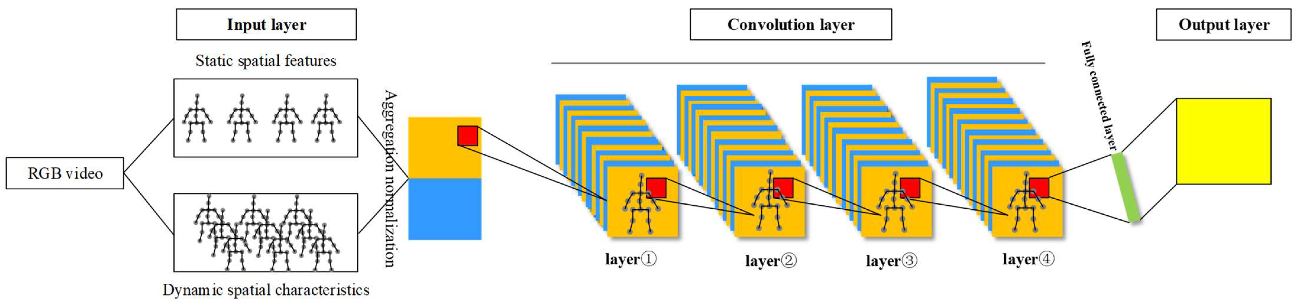
(2) The input layer serves as the initial layer in the CNN architecture, facilitating the introduction of data into the neural network. In Convolutional Neural Networks (CNNs), the primary role of the input layer is to receive and prepare raw grid-structured data, such as images. For colored images, the input layer typically handles a three-dimensional array with dimensions (height, width, and channel count). In the case of RGB images, there are three channels, representing red, green, and blue, respectively, while grayscale images consist of a single channel. Prior to propagation through the network, image data are commonly normalized, converting each pixel value to a range between [0, 1], which aids in expediting the model’s convergence.

The input of the network layer is video frame data with helmet feature point information. Firstly, the static feature of the human motion space attitude is extracted from the image containing feature points, and then, the hidden dynamic feature is obtained by the position transformation of the same joint point of two video frames under Δt time difference. The network diagram of the process is shown in Figure 1.

Specifically, the spatial flow defines a single action as p in the process of extracting information, the total number of action sequences is T, the individual time is t (t ∈ T), and its action feature is $f_i^p(i)$. Now, the information obtained by the network layer in the feature extraction process is integrated, and the sequence values of each frame of action are aggregated and normalized; that is, the maximum and minimum values obtained during the change of the joint vector i of the action are integrated.

$$h_i=\min f_i^p(i)$$

(1)

$$H_i=\max f_i^p(i)$$

(2)

The set of all static features is represented as

$$V_{\mathrm{stat}}^p=\left[h_1,h_2,\cdots ,h_m;H_1,H_2,\cdots ,H_m\right]$$

(3)

where $V_{\mathrm{stat}}^p$ denotes the static feature of the video sequence.

The dynamic features of human spatial pose motion are represented by the sequence difference of joint point data in adjacent video frames. Let the difference between adjacent intervals be $\mathsf{\Delta }{f}_t^p$, then $\mathsf{\Delta }{f}_t^p=f_{t+\mathsf{\Delta }t}^p-f_t^p$, which can be integrated into m − 1 corresponding data values in m video frames as hidden features to enhance the static spatial pose data. The process can be expressed as

$$V_{\mathrm{dyn}}^p=\left[\mathsf{\Delta }{h}_1,\mathsf{\Delta }{h}_2,\cdots ,\mathsf{\Delta }{h}_{m-1};\mathsf{\Delta }{H}_1,\mathsf{\Delta }{H}_2,\cdots ,\mathsf{\Delta }{H}_{m-1}\right]$$

(4)

(3) The pooling layer is designed to reduce the dimensionality of the output from the convolutional step (feature maps), both diminishing the size of the model and retaining crucial information within this reduced model. Pooling layers are typically situated between two convolutional layers, with each pooling layer’s feature map connected to its preceding convolutional layer’s feature map, hence maintaining an equivalent number of feature maps. The primary pooling operations are max pooling and average pooling, with max pooling being more prevalently utilized.

(4) The fully connected layer abstracts image data into a one-dimensional array. After undergoing processes through two rounds of convolutional and pooling layers, the final classification result in a Convolutional Neural Network is delivered by three fully connected layers. The transition from either a convolutional or pooling layer to a fully connected layer necessitates a “Flatten” layer that linearizes multidimensional inputs. The first fully connected layer, denoted as “fullc-1”, receives its input from the output of the “pooling-2” layer, transforming this node matrix into a vector. The purpose of the dense layer is to take the previously extracted features and, through nonlinear transformations in the dense layer, capture the relationships among these features, eventually mapping them onto the output space.

2.2. TS-LSTM

In real-world action detection, relying solely on the spatial flow convolution to extract human body information often falls short in accurately representing the entirety of the action features. This limitation becomes particularly evident when trying to differentiate actions that are similar in nature. To overcome this, we introduce a temporal layer network that meticulously extracts the temporal dynamics present within the motion. This is achieved by combining the features derived from both the spatial and temporal flows, providing a more comprehensive understanding of the action.

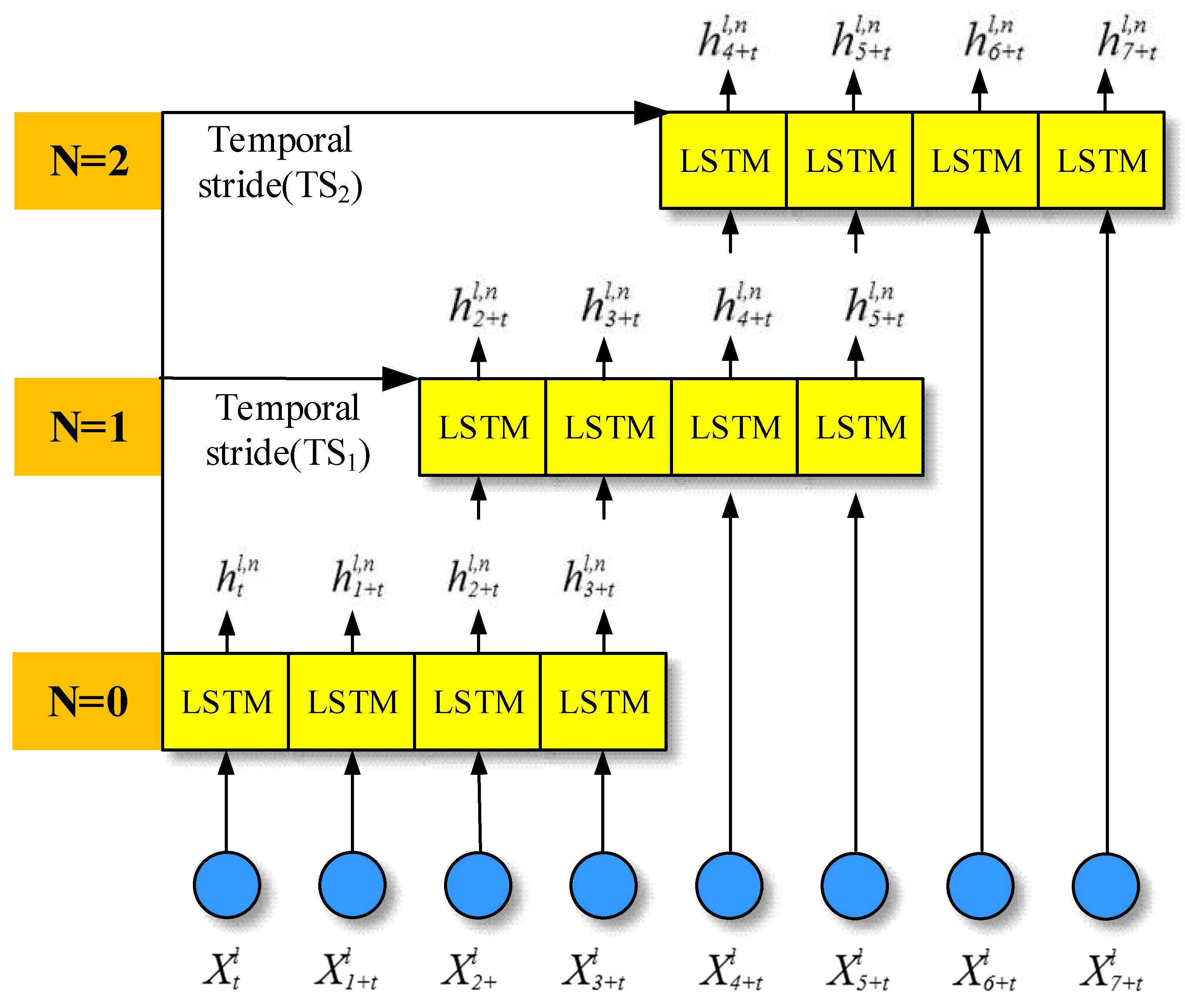
The long short-term Memory (LSTM) network, an advanced variant of the recurrent neural network, has gained traction for modeling time series data, especially in the domain of human behavior recognition [23,24]. Traditional LSTM networks, while effective, primarily capture global time dynamics. This overarching approach often overlooks intricate temporal nuances, sidelining potentially crucial details pivotal for precise action recognition. Recognizing this gap, our research innovates upon the conventional LSTM. We introduce an enhanced time stream sliding LSTM mechanism, complete with three cyclic modules catering to long-term, medium-term, and short-term memory. This design emphasizes capturing local joint information with heightened precision. Utilizing a sliding window mechanism, our model sequentially extracts skeletal timing data, effectively synthesizing it into the action’s attribute profile. A visual representation detailing the sliding operation process is elucidated in Figure 2.

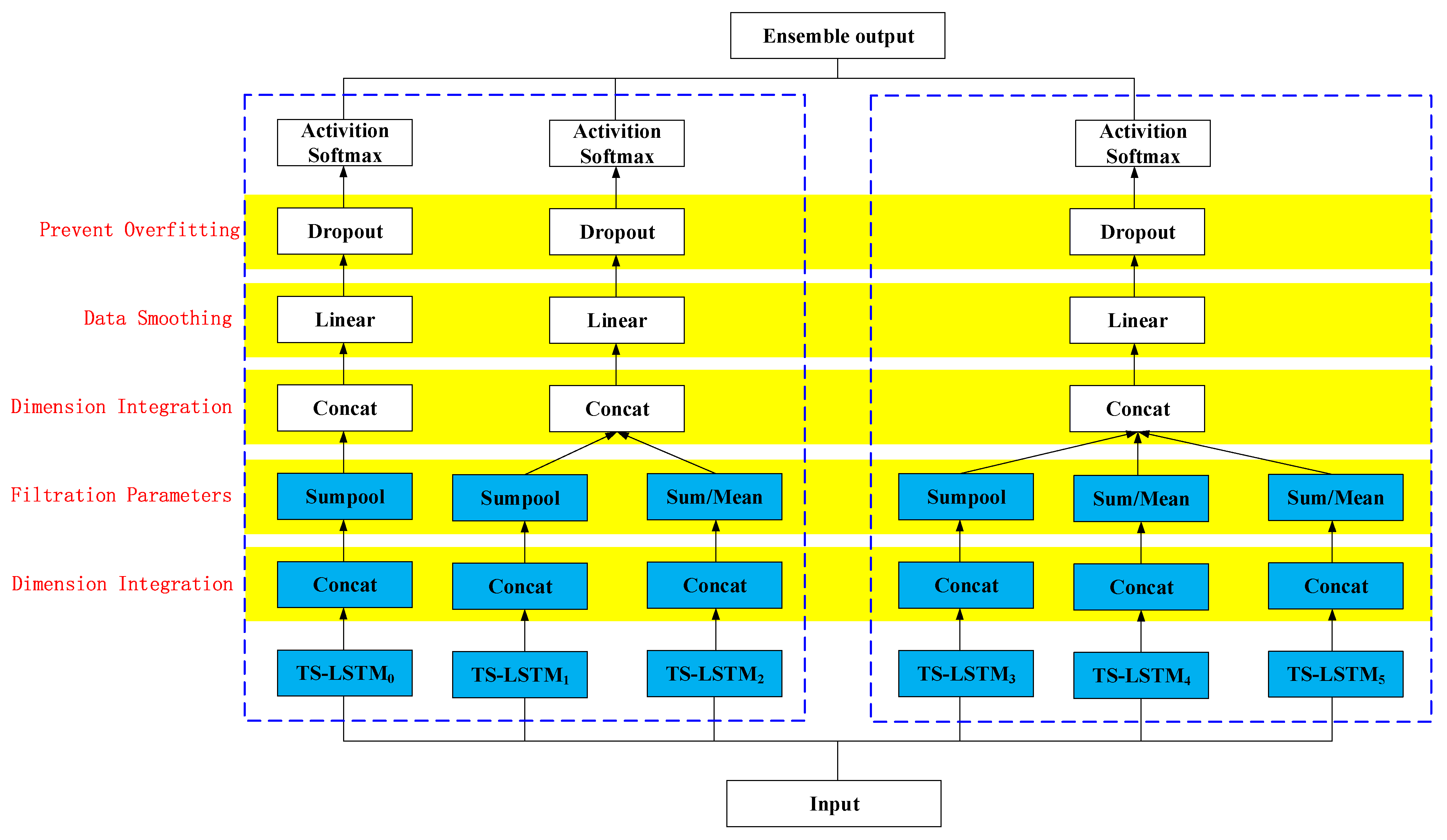
The improved TS-LSTM module is shown in Figure 3. The model is composed of three modules in the long and short term and adds a Concat layer, Sumpool layer, Linear layer, and Dropout layer to enhance the ability of feature extraction. The function of the Concat layer is to integrate the dimensions of the output data of the TS-LSTM layer, the Sumpool layer and the Meanpool layer are used to filter irrelevant parameters to prevent the network from overfitting during training, and the Linear layer is a fully connected layer that is used to smooth the data and integrate the local features extracted by different neurons into complete human skeleton motion information. The Dropout layer is used to prevent the parameters of the previous layer from overfitting and stop the invalid part of the neurons from working. The parameters of the three cycles of the network in this paper are determined by the proportion of the number of channels and one in the TS-LSTM unit in each module. Because there is only one channel in the first module, the number of cycles is one, the period of each channel in the second module is 0.5, and the period of each channel in the third module is 0.33.

The number of LSTM is set to N_l, its sliding window is set to W_l, and the time step is set to TS_l. Different LSTM units form different sliding windows, and more efficient feature extraction is achieved by adjusting the size of the sliding window and the time step. Assuming that $O{X}_t^l$ is the output of the lth unit layer at time t, the output and three gates of the LSTM unit can be expressed as

$$i_t^{l,n}=\sigma \left({\mathit{W}}_{ix}^{l,n}O{X}_t^{l,n}+{\mathit{W}}_{i,h}^{l,n}{h}_{t-1}^{l,n}+b_i^{l,n}\right)$$

(5)

$$f_t^{l,n}=\sigma \left({\mathit{W}}_{fx}^{l,n}O{\mathit{X}}_t^{l,n}+{\mathit{W}}_{fh}^{l,n}{h}_{t-1}^{l,n}+{\mathit{b}}_f^{l,n}\right)$$

(6)

$$c_t^{l,n}=f_t^{l,n}{c}_{t-1}^{l,n}+i_t^{l,n}\tanh \left({\mathit{W}}_c^{l,n}\mathit{O}{\mathit{X}}_t^{l,n}+{\mathit{W}}_{ch}^{l,n}{\mathit{h}}_{t-1}^{l,n}+{\mathit{b}}_c^{l,n}\right)$$

(7)

$${\mathit{o}}_t^{l,n}=\sigma \left({\mathit{W}}_{ox}^{l,n}\mathit{O}{\mathit{X}}_t^{l,n}+{\mathit{W}}_{oh}^{l,n}{\mathit{h}}_{t-1}^{l,n}+{\mathit{b}}_o^{l,n}\right)$$

(8)

In the formula, $i_t^{l,n}$ is the input gate, $f_t^{l,n}$ is the forgetting gate, ${\mathit{o}}_t^{l,n}$ is the output gate, $c_t^{l,n}$ is the activation unit, $h_{t-1}^{l,n}$ is the output of the unit, $W_{mn}^{l,n}$ is the connection weight matrix of the nth unit to the mth unit in the l-layer TS LSTM, and the update formula of each LSTM unit is:

$$h_t^{l,n}=o_i^{l,n}\tanh \left(c_i^{l,n}\right)$$

(9)

Next, let the mth time series input be ${\mathit{X}}_t^l$, which is expressed as ${\mathit{X}}_t^{l,m}$ and substituted into Formulas (6)–(9). Similarly, $h_t^{l,n}$ is expressed as $h_t^{l,n,m}$ and substituted into Formula (10).

$$q_{\mathrm{S}}^{l,m}=\sum _{t=0}^{w_l-1}concat\left({\left[h_{n^{\ast }T{S}_{t+i}}^{l,n,m}\right]}_{n=0}^{n=N_t-1},0\right);{((\cdot )]}_{n=0}^{n=N_t-1}=[\left(\cdot h_0{(\cdot )}_1\cdots {(\cdot )}_{N_l-1}\right)$$

(10)

$$q_{\mathrm{M}}^{l,m}=\frac{q_{\mathrm{S}}^{l,m}}{W_l}$$

(11)

Expressions (11) and (12) represent the MeanPool value and the SumPool value of the nth unit in the l layer under the n time sequence, respectively. Then, it is connected in a series to obtain

$$\{\begin{array}{l}{r}_{\mathrm{S}}^m={\left[q_{\mathrm{S}}^{0,m}\right]}^{\mathrm{T}}\hfill \\ r_{\mathrm{M}}^m={\left[concat\left(\left[q_{\mathrm{S}}^{1,m},q_{\mathrm{S}}^{2,m}\right],1\right)\right]}^{\mathrm{T}}\hfill \\ r_{\mathrm{L}}^m={\left[concat\left(\left[q_{\mathrm{S}}^{3,m},q_{\mathrm{S}}^{4,m},q_{\mathrm{S}}^{5,m}\right],1\right)\right]}^{\mathrm{T}}\hfill \end{array}$$

(12)

The linear activation algorithm of the TS-LSTM module is given by Expressions (13)–(15).

$$a_{\mathrm{S}}^m=w_{\mathrm{S}}\cdot r_{\mathrm{S}}^m+b_{\mathrm{S}}$$

(13)

$$a_{\mathrm{M}}^m=w_{\mathrm{M}}\cdot r_{\mathrm{M}}^m+b_{\mathrm{M}}$$

(14)

$$a_{\mathrm{L}}^m=w_{\mathrm{L}}\cdot r_{\mathrm{L}}^m+b_{\mathrm{L}}$$

(15)

In the formula, w and b represent the weight and deviation of the linear layer, respectively. After activation, the kth action values of $a_{\mathrm{S}}^m$, $a_{\mathrm{M}}^m$, and $a_{\mathrm{L}}^m$ are set to $a_{\mathrm{S}}^{m,k}$, $a_{\mathrm{M}}^{m,k}$, and $a_L^{m,k}$, respectively, and finally, they are normalized.

$$\mathrm{Pr}\left(c\mid a_{\mathrm{S}}^m\right)=\frac{\exp \left(a_{\mathrm{S}}^{m,c}\right)}{{\displaystyle \sum _{k=0}^{N_c-1}}\exp \left(a_{\mathrm{S}}^{m,k}\right)}$$

(16)

$$\mathrm{Pr}\left(c\mid a_{\mathrm{M}}^m\right)=\frac{\exp \left(a_{\mathrm{M}}^{m,c}\right)}{{\displaystyle \sum _{k=0}^{N_c-1}}\exp \left(a_{\mathrm{M}}^{m,k}\right)}$$

(17)

$$\mathrm{Pr}\left(c\mid a_{\mathrm{L}}^m\right)=\frac{\exp \left(a_{\mathrm{L}}^{m,c}\right)}{{\displaystyle \sum _{k=0}^{N_c-1}}\exp \left(a_{\mathrm{L}}^{m,k}\right)}$$

(18)

N_c and c represent the number of action types and the index of the corresponding class, respectively. The maximum likelihood estimation of the sample using the cross-entropy function is shown in Equation (20).

$$e=-\sum _{m=0}^{N_M-1}\sum _{c=0}^{N_c-1}{y}_c^m\ln \{Pr\}$$

(19)

In the formula, N_M−1 and $y_c^m$ represent the total number of training samples and the actual action labels, respectively. In order to highlight the interclass gap caused by the different motion amplitudes of the same action, the minimum objective function is used to train it again, and the average value of the results of the three activation functions (16)–(18) is taken in the final test.

2.3. Fusion Strategy

Cross-entropy serves as a metric to gauge the discrepancy between two probability distributions. Given a true distribution P and a predicted distribution Q from the model, cross-entropy is defined as

$$H(P,Q)=-\sum _{i}P(i)\log Q(i)$$

(20)

where i refers to each potential category. In the realm of classification tasks, the genuine distribution P is often represented in a one-hot encoded fashion, implying that the probability for a singular category is 1, while it remains 0 for others.

Considering the mean squared error (MSE) loss function, it is defined as

$$MSE=\frac{1}{n}\sum _{i=1}^n{(P(i)-Q(i))}^2$$

(21)

where n denotes the number of categories. In comparison with cross-entropy, when the predictive values deviate substantially from the genuine labels, the growth rate of the MSE is relatively more gradual. Contrarily, cross-entropy penalizes misclassifications more heavily.

Delving into the dual-stream network, $y_{ct}$ and $y_{cs}$ respectively represent the predicted probabilities from the spatial and temporal streams. The objective of the fusion strategy is to identify an optimal weight λ that amalgamates these predictions, aiming for the best comprehensive prediction $y_c$. Employing cross-entropy, the fusion loss can be articulated as

$$H_{\mathrm{fusion}}=-\sum _{i}P(i)\log \left(\lambda \frac{1}{n}\sum _j{y}_{ct}(j)+(1-\lambda )\frac{1}{n}\sum _j{y}_{cs}(j)\right)$$

(22)

Before obtaining the final output, it is necessary to perform spatiotemporal fusion on the two-stream network. The loss function uses the cross-entropy function to obtain the probability that the current prediction sample belongs to all categories. The specific calculation method is

$${\widehat{y}}_c=\lambda \frac{{\displaystyle \sum _n}{\widehat{y}}_{ct}}{n}+(1-\lambda )\frac{{\displaystyle \sum _n}{\widehat{y}}_{st}}{n}$$

(23)

In the formula, ${\widehat{y}}_{ct}$ and ${\widehat{y}}_{st}$ are the prediction probability vectors of the space flow and the time flow for the current input, respectively, and λ is a constant of (0–1). In order to find a more appropriate λ value, the problem is described as a simple optimal solution value problem. The particle swarm optimization algorithm is used to obtain the most suitable solution to the problem by using different λ values.

2.4. Feature Extraction Method

More unsafe behaviors in the construction industry are people’s unsafe behaviors. Through the investigation of production safety accidents in the construction industry, most production safety accidents are caused by not wearing safety protection appliances, illegal operations, and breaking through safety protections. Among them, not wearing safety protection appliances is the main cause of accidents, while breaking through safety protections and being close to dangerous areas are secondary causes. Therefore, according to the definitions of the three unsafe behaviors, the unsafe behaviors of construction workers are identified from three aspects: safety protection appliance detection, human dangerous actions, and personnel detection in dangerous areas.

The Faster R-CNN-LSTM network framework consists of two parts: RPN (candidate box extraction) uses a fully Convolutional Neural Network to extract candidate boxes, and the detection module uses the proposal window extracted by RPN to classify and regress the targets. The RPN structure is shown in Figure 4. The basic idea is to find all possible candidate regions in the feature map.

2.5. Loss Function

In complex operational scenarios, the primary objective of the loss function is to address the imbalance between positive and negative samples in the safety helmet dataset. To tackle this challenge, during the training process, samples are assigned varying weights based on their level of difficulty. Weights of simpler samples are reduced, while those of more challenging samples are increased, thereby enhancing the model’s discriminative capability.

$$L=-y\log (p)-(1-y)\log (1-p)$$

(24)

In the formula, L is the cross-entropy loss function, p is the probability that the predicted sample belongs to 1, and y is the label, such as [−1, 1]. The Focal loss function is as follows. To further address the imbalance between the positive and negative samples, the Focal loss function was employed. This loss function is an evolution of the cross-entropy loss function, incorporating modulating coefficients and balancing factors to better handle challenging samples. It is defined as follows:

$$L_f=-\alpha {(1-p)}^{\gamma }y\log (p)-(1-y)p^{\gamma }\log (1-p)$$

(25)

L_f is the Focal loss functio, γ is the adjustment coefficient, and α is the balance factor.

The Focal loss function adds an adjustment coefficient compared to the cross-entropy loss function, which reduces the loss of a large number of simple samples by making γ > 0, so the model is more focused on the mining of difficult samples. In addition, the balance factor α is added to solve the problem of class imbalance in the dataset.

3. Network Model Based on Faster R-CNN-LSTM

3.1. Structure Feature Extraction Strategy

With the proliferation of camera installations across construction sites, advancements in data collection speed, information processing capabilities, and swift transmission have been realized. Such progress furnishes an expansive data trove, brimming with images of construction personnel donned in protective gear. Capitalizing on this, our study harnesses site surveillance footage, further augmented with web crawler technology, focusing on a quintessential safety accessory: the safety helmet.

Utilizing the TensorFlow framework, this paper endeavors to discern the adherence to safety helmet usage among construction workers. Our methodology commences with a meticulous collection of images, capturing workers both with and without safety helmets across a plethora of intricate operational backdrops. Once acquired, these images undergo pre-annotation and are segmented to align with the training prerequisites of the Faster R-CNN-LSTM network framework. In light of the initial training and test results, tweaks are made to the Faster R-CNN-LSTM framework, fostering iterative refinements. This iterative process culminates in target detection that satisfactorily meets the accuracy benchmarks. A schematic representation of the safety helmet identification procedure can be glimpsed in Figure 5.

3.2. Dataset Construction

The complex operation of the building site is defined as two operation modes. One is that multiple operation groups work on the same operation object in different areas at the same time. The second is a series operation of multiple operation objects in the same area at different times by a single operation group. Complex operations include two types of operations: parallel operations and vertical operations. Complex operations are composed of four characteristics: personnel organization, time, operation object, and operation location. The formation process is shown in Figure 6; the black solid arrow is the formation process of parallel operations, and the black virtual arrow is the formation process of vertical operations.

With the popularity and wide application of cameras in construction sites, this paper uses video surveillance at the sites of construction projects to collect the situation of construction workers wearing safety helmets under complex operating conditions. In this paper, a total of 7581 images were collected, including wearing a helmet (positive class) and not wearing a helmet (negative class), as shown in Figure 7.

3.3. Experimental Settings and Evaluation Metrics

The dataset was annotated with the Labellmg annotation tool, and the annotation results were saved as an XML file in VOC format, which can be called python. In this paper, a safety helmet dataset under complex operation scenarios is established, and an improved Faster R-CNN safety helmet detection method is proposed; three sets of anchor points are added to detect small target safety helmets, combining Focal loss instead of the original loss function to solve the problem of class imbalance in the dataset, and the improved strategy further improves the accuracy of helmet recognition in complex job scenarios.

The number of anchor points is an important hyperparameter in RPN. The anchor points are located in the sliding window, which directly affects the generation of feature maps. There are nine anchor points in the original Faster R-CNN network framework; that is, three sizes and three aspect ratios, determining the position of the current sliding window and the corresponding candidate region. However, in the complex operation scenario, the safety helmet belongs to the category of small targets, and the default nine anchor points make it difficult to recall the safety helmets of small targets, which, in turn, affects their subsequent classification and regression. Therefore, this paper adds three groups of anchor points (smaller than the default value) onto the basis of the original network framework, so that it can detect the helmets of small targets, improve the detection ability, and increase the number of detections.

The images labeled by Labellmg are input into the improved CNN-LSTM network framework for training. Validate all the data, and assign the training set. The 7581 labeled and classified images are divided into four categories according to the VOC2007 format. The results of the image data division of helmet detection are shown in

Table 1. Safety helmet detection image dataset division.

Data Type	Number of Samples
Training set	5457
Vertify set	607
All set	6064
Test set	1517

.

3.4. Model Evaluation

AP (average precision) is a comprehensive measure of accuracy and recall rate. It first calculates the accuracy rate of each category and then calculates the average accuracy of each category.

$$P_i=\frac{n_{pi}}{n_0}$$

(26)

In the formula, P_i is the accuracy rate, n_pi is the true number of i-type pictures, and n₀ is the number of all targets for the dataset category i.

$$A{P}_i=\frac{\sum P_i}{n_t}$$

(27)

In the formula, $\sum P_i$ is the sum of the accuracy, and n_t is the number of images that contain category i targets.

The mean average precision (MAP) measures the pros and cons of each category in the model for all the detection categories.

$$MAP=\frac{\sum A{P}_i}{N}$$

(28)

In the formula, MAP is the average accuracy, $\sum A{P}_i$ is the sum of the average accuracy, and N is the number of all classes.

3.5. Test Process and Results

In the training process of Faster R-CNN, SGD is typically employed as the optimizer, with an initial learning rate set at 0.001, momentum at 0.9, and weight decay of 0.0005. For the LSTM training, the Adam optimizer is commonly adopted, with an initial learning rate of 0.001, incorporating a dropout rate of 0.5 for model regularization. To prevent overfitting and ensure the timely termination of the training, the process is halted if the loss in the validation set does not show significant improvement over 20 consecutive epochs. This strategy ensures that the model achieves the optimal training results without compromising its generalization capabilities. The original Faster R-CNN-LSTM network framework and the improved Faster R-CNN network framework are trained using the safety helmet dataset under complex operation conditions. As shown in Figure 8, after the unimproved Faster R-CNN-LSTM network framework is iterated to 80,000 times, the loss value tends to converge, and the loss value is 0.8. The improved Faster R-CNN-LSTM network structure converges into 0.2 after 50,000 iterations. The improved network framework can effectively reduce the loss value and optimize the network structure.

After the training is completed, the model accuracy of the two network frameworks is evaluated, and the best effect MAP of the two algorithms is shown in

Table 2. Model comparisons.

Methods	Wear a Helmet AP	Not Wear a Helmet AP	MAP
CNN-LSTM	0.7515	0.4878	0.6197
Faster R-CNN-LSTM	0.8084	0.7386	0.7735

.

From the data presented in Table 2, we observe that the mean average precision (MAP) of the refined Faster R-CNN-LSTM framework surpasses that of the conventional CNN-LSTM framework by a significant 15%. The respective detection outcomes from both methods are further examined in Figure 9. In our experiments, the CNN-LSTM model detected four instances correctly with one instance misclassified, culminating in an average detection accuracy of 91.48%. Conversely, the enhanced Faster R-CNN-LSTM model demonstrated impeccable performance with a flawless detection rate, achieving a remarkable accuracy of 99.99%. These results substantiate the proficiency of the improved Faster R-CNN-LSTM framework, especially in recognizing small target helmets, thus underscoring its capability to bolster the overall network performance.

Further analysis of the model’s recognition accuracy was conducted by comparing the recognition results in complex environments, as illustrated in Figure 10. The CNN-LSTM network framework detected five instances, exhibited one false detection, and had one miss. In contrast, the improved Faster R-CNN network framework showed no false detections or misses, indicating its superior recognition accuracy. As depicted in Figure 8, a comparison of the two models’ recognition abilities can be observed with the individual on the far right of the image. The CNN-LSTM tends to misidentify individuals wearing regular hats as those wearing safety helmets. The enhanced model, on the other hand, exhibits a greater accuracy in recognizing the edge features of safety helmets, accurately determining whether individuals are donning safety helmets.

Besides the baseline Faster R-CNN model, our research juxtaposes its performance against variants of the Faster R-CNN employing different feature extraction networks.

Table 3. Model comparisons.

Model	MAP
CNN-LSTM	0.619
SE-ResNET50	0.702
VGG16	0.646
Faster R-CNN-LSTM	0.773

delineates the detection efficacy of these diverse extraction networks. Evidently, the network framework deployed in this study stands out, with a MAP score of 0.773, reflecting a commendable 15% augmentation when contrasted with the foundational network framework.

4. Discussion

In this study, we introduced and tested a dual-stream convolutional model for hazardous behavior recognition based on Faster R-CNN-LSTM. The primary advantage of this model lies in its ability to holistically consider spatiotemporal features by integrating the spatial characteristics of Faster R-CNN with the temporal properties of LSTM. This integration provides a more comprehensive perspective for behavior recognition. The experimental results affirmed its high accuracy in recognizing unsafe behaviors, especially in classifying whether construction workers wear safety helmets. Additionally, the model is equipped with the capability to process video streams in real time, offering instantaneous safety monitoring on construction sites.

However, due to the amalgamation of two network structures, the computational complexity of the model is relatively high, which might lead to increased computational resource demands. The model could also face the risk of overfitting when the dataset is limited, potentially diminishing its generalization capacity in practical applications.

Two pivotal areas emerge for future improvements: (1) The model’s structure can be further refined to reduce the computational resource requirements and enhance its efficiency. (2) There is potential in integrating other types of sensor data, such as audio or temperature, to furnish the model with richer contextual information, thereby further improving its recognition accuracy.

In terms of practical applications, this model boasts significant potential. It can be implemented on construction sites to provide the real-time monitoring of workers’ behaviors, allowing for early detection and warnings of potential unsafe actions. By analyzing and evaluating workers’ behaviors, the model can also serve as a robust data support for safety training initiatives on construction sites.

5. Conclusions

This study introduces an innovative approach to enhance the traditional two-stream convolution model. The proposed “Two-Stream Convolution Danger Recognition Model based on CNN-LSTM” effectively integrates the strengths of both CNN and LSTM networks. Within this synergy, the CNN network, acting as the spatial stream, is finely tuned to extract spatial motion posture information from the human body. Concurrently, in the temporal stream, an improved TS-LSTM network is employed to amplify the model’s temporal feature extraction capability.

This innovative fusion yields promising outcomes. A notable 15% increase in the MAP was observed, signifying a substantial enhancement in the model’s accuracy in pinpointing unsafe behaviors. This improvement holds profound practical implications. In environments such as construction sites, the enhanced model can significantly reduce risks for workers by adeptly identifying potential hazards.

To validate the model’s credibility and robustness, it underwent rigorous testing using four distinct verification methods. Across all tests, the results consistently underscored the high accuracy of the Faster R-CNN-LSTM network framework. Particularly in complex settings, the improved Faster R-CNN-LSTM excels, especially in recognizing edge features of safety helmets. Simultaneously, when compared to models with other feature extraction networks, the framework utilized in this study distinctly outperforms, achieving a MAP of 0.773. In essence, this research successfully elevates the model’s recognition accuracy and robustness, offering powerful technical support for safety monitoring in intricate environments like construction sites.

References

1. Chen, S.; Cheng, K.; Yang, J.; Zang, X.; Luo, Q.; Li, J. Driving Behavior Risk Measurement and Cluster Analysis Driven by Vehicle Trajectory Data. Appl. Sci. 2023, 13, 5675. [Google Scholar]
2. Hou, L.; Chen, H.; Zhang, G.; Wang, X. Deep Learning-Based Applications for Safety Management in the AEC Industry: A Review. Appl. Sci. 2021, 11, 821. [Google Scholar]
3. Lattanzi, E.; Castellucci, G.; Freschi, V. Improving Machine Learning Identification of Unsafe Driver Behavior by Means of Sensor Fusion. Appl. Sci. 2020, 10, 6417. [Google Scholar]
4. Guo, H.; Liu, W.; Zhang, W.; Skitmor, M. A BIM-RFID Unsafe On-Site Behavior Warning System. In Proceedings of the 2014 International Conference on Construction and Real Estate Management, Kunming, China, 27–28 September 2014. [Google Scholar]
5. Tong, R.; Cui, P. Unsafe factor recognition and interactive analysis based on deep learning. China Saf. Sci. J. 2017, 27, 49–54. [Google Scholar]
6. Dan, X.U.; Yong, D.; Junhong, J. Research on driver behavior recognition method based on convolutional neural network. China Saf. Sci. J. 2019, 29, 12–17. [Google Scholar]
7. Tong, P.; Zhang, Y. Integration between artificial intelligence technologies for miners’ unsafe behavior identification. China Saf. Sci. J. 2019, 29, 7. [Google Scholar]
8. Wang, Z.; Zhao, Y. Construction Workers’ Unsafe Behavior Research Analysis and Evaluation Model. Acta Anal. Funct. Appl. 2015, 17, 198–208. [Google Scholar]
9. Girshick, R.; Donahue, J.; Darrell, T.; Malik, J. Region-based convolutional networks for accurate object detection and segmentation. IEEE Trans. Pattern Anal. Mach. Intell. 2015, 38, 142–158. [Google Scholar]
10. Girshick, R. Fast r-cnn. In Proceedings of the IEEE International Conference on Computer Vision, Santiago, Chile, 7–13 December 2015; IEEE: Piscataway, NJ, USA, 2015; pp. 1440–1448. [Google Scholar]
11. Ren, S.; He, K.; Girshick, R.; Sun, J. Faster R-CNN: Towards real-time object detection with region proposal networks. IEEE Trans. PatternAnalysis Mach. Intell. 2017, 39, 1137–1149. [Google Scholar]
12. Redmon, J.; Divvala, S.; Girshick, R.; Farhadi, A. You only look once: Unified, real-time object detection. In Proceedings of the IEEE Conference on Computer Vision and Pattern Recognition, Las Vegas, NV, USA, 26 June–1 July 2016; IEEE: Piscataway, NJ, USA, 2016; pp. 779–788. [Google Scholar]
13. Hu, T.; Wang, X. Analysis and Design of Safety Helmet Identification System Based on Wavelet Transform and Neural Network. Softw. Guide 2006, 26, 37–39. [Google Scholar]
14. Fang, Q.; Li, H.; Luo, X.; Ding, L.; Luo, H.; Rose, T.M.; An, W. Detecting non-hardhat-use by a deep learning method from far-field surveillance videos. Autom. Constr. 2018, 85, 1–9. [Google Scholar] [CrossRef]
15. Zhang, M.; Cao, Z.; Zhao, X.; Yang, Z. Research on Construction Worker Safety Helmet Wearing Recognition Based on Deep Learning. J. Saf. Environ. 2019, 19, 535–541. [Google Scholar]
16. Wu, D.; Wang, H.; Li, J. Safety Helmet Detection and Identity Recognition Based on Improved Faster RCNN. Inf. Technol. Informatiz. 2020, 1, 17–20. [Google Scholar]
17. Wang, B.; Li, W.; Tang, H. Improved YOLO v3 Algorithm and Its Application in Safety Helmet Detection. Comput. Eng. Appl. 2020, 56, 33–40. [Google Scholar]
18. Aiadi, O.; Khaldi, B.; Saadeddine, C. MDFNet: An unsupervised lightweight network for ear print recognition. J. Ambient. Intell. Humaniz. Comput. 2023, 14, 13773–13786. [Google Scholar] [CrossRef]
19. Zhang, H.; Ma, C.; Pazzi, V.; Zou, Y.; Casagli, N. Microseismic Signal Denoising and Separation Based on Fully Convolutional Encoder–Decoder Network. Appl. Sci. 2020, 10, 6621. [Google Scholar] [CrossRef]
20. Xiao, S.; Nie, A.; Zhang, Z.; Liu, S.; Song, M.; Zhang, H. Fault Diagnosis of a Reciprocating Compressor Air Valve Based on Deep Learning. Appl. Sci. 2020, 10, 6596. [Google Scholar] [CrossRef]
21. Park, J.; Kim, J.K.; Jung, S.; Gil, Y.; Choi, J.I.; Son, H.S. ECG-Signal Multi-Classification Model Based on Squeeze-and-Excitation Residual Neural Networks. Appl. Sci. 2020, 10, 6495. [Google Scholar] [CrossRef]
22. Aiadi, O.; Khaldi, B.; Kherfi, M.; Mekhalfi, L.; Alharbi, A. Date Fruit Sorting Based on Deep Learning and Discriminant Correlation Analysis. IEEE Access 2022, 10, 79655–79668. [Google Scholar] [CrossRef]
23. Son, N.; Yang, S.; Na, J. Deep Neural Network and Long Short-Term Memory for Electric Power Load Forecasting. Appl. Sci. 2020, 10, 6489. [Google Scholar] [CrossRef]
24. Do, N.T.; Kim, S.H.; Yang, H.J.; Lee, G.S. Robust Hand Shape Features for Dynamic Hand Gesture Recognition Using Multi-Level Feature LSTM. Appl. Sci. 2020, 10, 6293. [Google Scholar] [CrossRef]
Figure 1. CNN-based action recognition.
Applsci 13 10700 g001
Figure 2. TS-LSTM model structure.
Applsci 13 10700 g002
Figure 3. TS-LSTM unsafe behavior recognition network structure.
Applsci 13 10700 g003
Figure 4. RPN structure.
Applsci 13 10700 g004
Figure 5. Safety helmet identification process.
Applsci 13 10700 g005
Figure 6. Complex task formation process.
Applsci 13 10700 g006
Figure 7. Examples of dataset pictures.
Applsci 13 10700 g007
Figure 8. Model loss comparisons.
Applsci 13 10700 g008
Figure 9. Comparison of monitoring effects. (a) CNN-LSTM. (b) Faster R-CNN-LSTM.
Applsci 13 10700 g009
Figure 10. Comparison of complex environment models. (a) CNN-LSTM. (b) Faster R-CNN-LSTM.
Applsci 13 10700 g010