Modeling of Pipe Whip Phenomenon Induced by Fast Transients Based on Fluid–Structure Interaction Method Using a Coupled 1D/3D Modeling Approach

Abstract

The sudden increase in the operating pressure of nuclear power plants (NPPs) is due to the water hammer phenomenon, which tends to produce a whipping effect that causes serious damage to the pipes and their surroundings. The mechanical response of these pipelines under the influence of such fast fluid transients can be estimated using the fluid–structure interaction (FSI) method. The computational time and expense are predominantly dependent on the number of finite elements developed in the model. Hence, an effective modeling technique with limited and efficient nodes and elements is desired to obtain the closest possible results. A coupled 1D/3D finite element modeling approach using the FSI method is proposed to determine the influence of fast transients on the mechanical pipe whipping behavior of gas pipelines in NPPs. The geometric coupled modeling approach utilizes the presence of both the 3D solid elements and the 1D beam elements sharing a local conjunction. The computational model is modelled for a pipe-to-wall impact test scenario taken from the previously conducted French Commissariat a l’Energie Atomique (CEA) pipe whip experiments. The results of displacement, stresses, and impact velocity at the 3D section featuring the elbow are compared for the change in the 3D solid length varied at the juncture of the elbow. The computed results from the Ansys FSI coupling method using the Fluent and Transient Structural modules provides fair validation with the previously conducted experimental results and correlates with the CEA pipe whip tests on pipe-to-wall impact models. Thus, the 1D/3D coupled modeling approach, which minimizes the area of the solid region by constricting it to the impact area with appropriate contact modeling at the junctures, can be considered in the future for decreasing the computational time and the creation of finite elements.

1. Introduction

Research on pipe whipping phenomenon is restricted to certain analytical and experimental methods, and the development of numerical methods are limited to intricate finite element models owing to the complexity of the structural dynamics of the analyses. The French Commissariat a l’Energie Atomique (CEA) conducted several experimental tests in their laboratory in the 1980s to analyze the pipe whip phenomenon. These tests were oriented towards the safety assessment of NPP’s installments the with development of structural safety methods for nuclear components. The safety assessment of the piping systems of the NPPs is crucial in preventing major loss due to structural impacts. The propagation of such damage should be critically analyzed to prevent derivative failures based on such inevitable events. The CEA put forth much effort in the development of nuclear safety engineering and other such related safety issues with advancing experimental and numerical models through applied research [1].

1.1. Background of Pipe Whip Tests

The French CEA along with the FRAMATOME agency has carried out several dynamic tests on nuclear piping financed by the Electric Power Research Institute (EPRI). The experimental tests on pipe impacts were performed in the Cadarache Laboratory in France. The main objective of these tests was to determine the effect of impact on the surrounding structures and piping systems in the NPPs and to assess the safety of the related components and structures for the development of the power plants for future applications.

The restraining system of the piping in the NPPs are known to be developed using a conservative approach and, hence, various structural parameters, like material non-linearity and large displacements, are often neglected in the restraint design methodology. An intricate restraint design would be expensive as well as redundant in certain cases. Therefore, studying the whipping behavior and the large displacements of NPP pipes during failure conditions would be beneficial in developing the restraint technology and assessing the surrounding structural damage [2].

The experimental tests proved to be expensive and complex owing to the intricacy of the operating conditions and the testing procedure. Due to this, several numerical methods and finite element models were developed over time to replicate the experimental tests. However, computational models are also sometimes computationally expensive and difficult to model with such operating conditions and demand coherence with the experimental models [3]. Several finite element codes have simulated the pipe whipping behavior by incorporating beam and shell elements with linear spring behavior using ABAQUS-EPGEN (Version 4.5), EUROPLEXUS-2005, and TEDEL (CEASEMT-V1) codes [2,4,5]. These codes use an explicit numerical algorithm to solve large deformations, fast dynamics, and strain rate-related problems.

The pipe whipping behavior as simulated in the previous research using computational tools does not justify the effect of material non-linearity and the pipe response to fluidic forces in three-dimensional models incorporating the fluid–structure interaction method without compromising the computational time. Computational time and feasibility have become major concerns with the advancement of numerical models for fast dynamics problems. These explicit models can alternatively be conservative and redundant depending on the complexity of the analysis and loading conditions. Hence, simpler and more efficient finite element models are preferred over complicated models.

Several attempts have been made to simplify the finite element models to achieve feasibility and solve complex explicit problems without compromising the accuracy. These developed numerical models are validated with the experimental results from time to time to evaluate their degree of acceptability [3,5,6,7].

This research applies the functions of both finite volume method (FVM) and finite element method (FEM) to solve large displacement problems of pipe whipping phenomenon with a simplified modeling approach by using a coupled one-dimensional and three-dimensional (1D/3D) numerical model. The fluid–structure interaction (FSI) methodology of the Ansys Workbench software is applied in this research to predict the response of the pipe under transient loading conditions.

The FSI methodology can be classified as one-way or two-way depending upon the coupling approaches integrated in the simulation. The one-way FSI approach uses the fluidic loads from the FVM simulation as the input load for the structural simulation whereas the two-way FSI approach includes the flow changes due to the structural deformations caused by the fluid forces from the FVM simulations, and the cycle continues. The two-way FSI approach is deemed to be computationally expensive, while the one-way FSI is conservative, as per the previously conducted research [8,9]. However, the one-way FSI approach is solved in this research, owing to the very small duration of the whipping event (milliseconds) with no significant changes disrupting the fluid flow [2,4,5,6].

1.2. Pipe Whip Based on Water Hammer Effect

Water and steam are the predominantly used fluid components in the nuclear power systems for their cooling and heating functions, respectively, since the working medium follows a thermodynamic cycle [10]. Some of the steam during the physical flowing process experiences a phase transition by condensing to water, causing a change in the flow. The change in flow inside a pipe creates a pressure difference inside the pipe, and the sudden pressure difference causes a cavitation effect where the absolute pressure waves of the fluid act on the walls of the pipe creating a dynamic load during the flow. Cavitation occurs at both the instances of high-pressure and low-pressure peaks inside the pipe [11,12].

During the four stages of cavitation, the pulsating pressure with bubble formation and collapse can sometime be fatal for the pipe and surroundings when vibrating at high pressure frequencies while affecting the strength and durability at lower frequencies. Such cavitations occur due to the fast fluid transients under dynamic conditions, eventually leading to a water hammer effect and, hence, the prevention of such fast fluid transients is of important consideration. Over the years, there has been a considerable amount of research conducted on the prevention of the water hammer effect, and various computational and analytical methods have been developed and demonstrated to minimize the fluid transients [13,14,15,16,17]. The method of characteristics (MOC) and the finite volume and the finite difference methods (FVM and FDM) are some of the classical methods for solving the water hammer effect with the use of partial differential equations (PDEs) and computational solvers [18]. The immersed boundary layer method (IBM) is another technique which uses feedback variables around the boundary to solve turbulent flows and intricate models. The computational grid is fixed and solved through Eulerian methods while the force is pointed towards the nodes of the Lagrangian grid. Computational accuracy can be enhanced by combining the lattice Boltzmann method (LBM) and IBM together by defining the boundary velocity through particle interactions. The fluid is defined as a body force in this method through Lagrangian force density by interpolating IBM and LBM, and a coupled approach between LBM and the FEM can be attained through FSI to solve complex models of fluid flow [19,20,21,22].

Research on water hammers under three variable states were studied previously, where they occurred as non-condensable gas-induced, column separated-induced, and condensed steam-induced water hammers. Under transient flow conditions, any disruption to the flow causes fluctuations which can result in severe rupture of the pipe. The classical approaches to solving the water hammer problems is to deal with the elastic vibrations of lower order frequencies assuming the pipes are linear elastic and thin-walled structures. Solving the wavefront model of the vibrating medium is another drawback of the linear models and, hence, MOC was used as an appropriate method. Several new approaches were demonstrated, eliminating the use of wavefronts and pipe lengths, and incorporating modern methods of recursions [23,24,25].

1.3. Applications of Numerical Codes for Pipe Whip Phenomenon

The modeling methodology for predicting the dynamic structural response of the high-pressure filled pipes for simulating the pipe whipping phenomenon is complex and develops significant data when the pressure–velocity coupling is considered. The simulation of water hammers using numerical tools has largely been conducted in recent years owing to the new methods of solving for various phenomena.

The computational fluid dynamics (CFD) studies are widely used to simulate valve closure effect while incorporating dynamic meshing techniques in ICEM. The various fluid parameters, like the velocity–pressure relationship, phase flows, and mass flow rate have been performed in the Ansys Fluent module over the years. Coupling the Fluent models with other numerical software is of major importance, as various solution methods solve multiple water hammer problems which can be a drawback in the classical methods.

The pressure induced in high-pressure pipes from the reservoirs and tanks during failure causes catastrophic effects in the nearby structures when the pipe undergoes fracture at operating conditions. The failure caused by such high-pressure fluid transients causes large displacements of the pipe when their free ends are not restrained appropriately. The water hammer effect can be modelled by considering the pressure and velocity of the flow inside the fluid by controlling a set of parameters in the fluid domain.

The structural response of the pipe due to fluid transients can be modelled using the fluid–structure interaction (FSI) method. The equilibrium between the solid and the fluid medium is considered during the FSI problem when the fluid forces cause a reaction force on the structure. The FSI model for solving impact behavior based on fast fluid transients was performed by Zhang et al. by considering the frequencies of the non-harmonic excitations, and they successfully solved the natural frequencies and mode shapes of the FSI model. The MOC-based frequency models with linear boundary conditions were attempted, and the major matrices were similar for the time-based arbitrary functions. Hamed et al. proposed a transfer matrix method for the FSI problem with a viscoelastic pipe with both Poisson and junction coupling models in the frequency domain. Riedelmeier et al., provided an oscillatory flow domain to determine the strength of a two-way coupling though variable excitation frequencies and validated it using numerical simulations [6,26,27,28,29].

The failure occurring at thermo-hydraulic conditions causes a whipping effect on the pipes and, hence, the appropriate modeling technique should be used with finite elements to define the non-linear behaviour of the material under transient conditions. Daude and Galon [30], proposed a finite volume method (FVM) approach based on Godunov model for solving compressible flows with both single- and two-phase media. A coupled model using FVM was solved for the governing equations of state for multi-dimensions for coupling one-dimensional (1D) and two-dimensional (2D) models. The time steps of the numerical simulations play a vital role in defining the equilibrium state and, hence, the Courant number should be satisfied considering the eigen frequency and the length of the beam and shell elements [6,30].

Computational time is one of the primary factors when modeling non-linearity and, hence, limited but efficient elements should be created in the domain of interest. The number of finite elements created in the domain of interest significantly affects the solution. The methodology used here is a coupled model containing both the one-dimensional (1D) beam elements and three-dimensional (3D) solid elements.

The results of the coupled modeling approach are validated with the experimental results conducted in the CEA’s Cadarache test facility [2,4].

2. Experimental Setup

2.1. CEA Pipe Whip Tests

This research deals with the validation of the simulated numerical models of the 1D/3D coupled system with the previously conducted French Commissariat a l’Energie Atomique (CEA) tests. Several CEA tests were conducted in the Cadarache Laboratory in France using the Aquitaine II steam facility to analyze the pipe whipping phenomenon. A total of 16 tests were performed under PWR conditions on the Schedule 80, 3-inch pipe, and they validated the pipe response with their numerical codes. These bulk tests were classified into two types based on the object of impact. The impact tests on stiff structural members and concrete slab were the two major considerations, with deviations in their gap dimensions [2,4,5].

Test 5 from the CEA experiments is compared with the numerical results of the presented modeling approach. The experimental results of test 5 are often considered a benchmark for validation of numerical models with its “pipe-on-wall-impact” scenario [2,4]. Test 5 includes a long pipe with an elbow made of French steel which has mechanical properties equivalent to that of A106 grade B steel. The experiment is carried out under controlled PWR conditions with the use of an explosive cord to initiate the instantaneous high-pressure flow or line break. The pipe is maintained at a temperature of about 300° Celsius and a pressure of around 16.6 MPa is maintained inside the pipe [2]. With such high operating pressures, the estimated duration of the tests was kept at 20 to 30 milliseconds (ms).

A typical experimental setup of the pipe is shown in Figure 1, where one end of the straight horizontal section of the pipe is attached to a water filled tank kept at operating pressure while the other end containing the elbow is kept unrestrained. A slab of concrete is kept fixed right below the elbow with a fixed gap where the pipe is expected to impact after a sudden high-pressure flow is initiated. The original experiments involved two major studies which included the mechanical response of the impacted slab during the pipe whipping effect and the measurement of the impact force on the slab. The large displacements of the whipping pipe are measured with a high-speed 5000 fps camera along with strain gauges kept on the rebars of the concrete slab to measure the impact parameters.

The deformation of the pipes in every experimental test depends on the geometry of the pipe, where the strain rate plays a vital role in the mechanical response of the pipe to the fluid transient. It is observed that the plastic strain is distributed uniformly along the length of the pipe for longer dimensions while localized plastic strain is present for shorter dimensions. Hence, the strain rate influence on the material behavior for the pipe whipping scenario can be neglected with reasonable justifications. The maximum impact force was observed in test 5 with a value of 385 kN and with a time to impact of 13.2 ms, as well as a localized crushing stiffness at the impact zone [4].

2.2. Previously Validated Research through Numerical Codes

Limited attempts were made with the numerical codes to model the pipe whip behavior and validate the obtained numerical data with the CEA tests. Garcia et al. [2] calculated the elastoplastic models of the CEA tests with the TEDEL numerical code. The dynamic pipe model is a simple pipe geometry with beam formulation modelled with a local linear stiffness at impact. The results found that this local stiffness greatly influences the pipe whip impact when compared to the strain rate, which can be neglected.

Hsu et al. [4] developed three modeling approaches using the Abaqus-EPGEN code with two models created completely with pipe and beam elements throughout the pipe. Two nodal beam and truss elements were modeled for the pipe, and a contact model based on a unidirectional gap element with a compression spring type was created between the pipe and the impacting slab. The impact on the slab is measured by the change in the gap closing of this element during the simulation process. The third model was created using a coupled modeling technique with beam elements modelled along the linear horizontal section of the pipe and shell elements at the elbow section of the pipe. The impact time, velocity, and forces were solved for the three models under controlled operating pressure and temperature. The ANSI 58.2 standard approach was used as a validatory tool to analyze the model parameters, and the results showed justifiable comparisons and suggested that the strain rate has a significant influence on the stiffness of the pipe when compared to the high-temperature pipe impacts.

With the developing FE codes, the versatility of such structural dynamic simulations should be presented from time to time with efficient models without compromising the computational accuracy and predictions. Simplified FE models are necessary for certain applications where the conservative approach is required with negligible changes to the accuracy of the solution. This research finds such model simplifications for the pipe whip tests where the dynamic response of the structural members is studied with a localized solid and beam modeling technique.

3. Computational Modeling Method

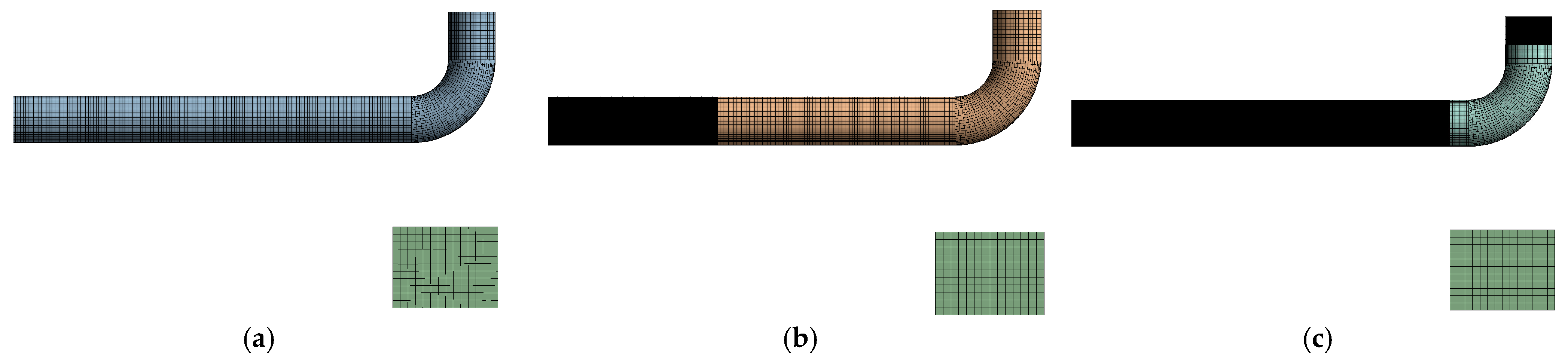
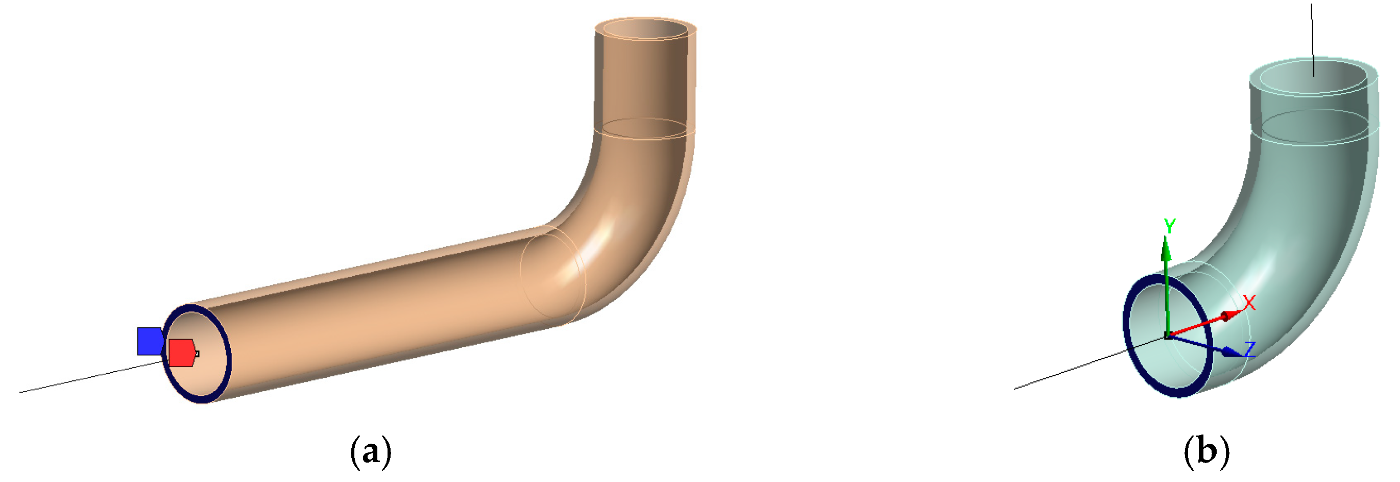
3.1. Pipe Whip Model

The pipe is modelled with a coupled 1D/3D modeling approach with three-dimensional solid elements created at the localized region of interest (elbow) of the pipe, and the rest of the horizontal length of the pipe is modelled with one-dimensional elements (Figure 1). These simplified models are then compared with a fully 3D model for simplified model verification. The design is based on the Aquitaine II pipe model layout as experimentally tested in the CEA tests [5]. The dimensions of the pipe model are taken from the standard Schedule 80 3″ pipe made of equivalent material to A106 grade B carbon steel.

The 3D elements are created in the region of the elbow where the pipe is expected to impact on the neighboring concrete slab kept at a distance of 200 mm from the longitudinal axis of the pipe. The solid elbow region of the pipe is modelled for two different pipe lengths of 550 mm and 150 mm to evaluate the structural response to the same failure conditions for predicting and comparing the computational time for the change in the number of elements. This research is dedicated to understanding the structural behaviour of simplified and localized 1D/3D coupled models under dynamic loading conditions through a fluid–structure interaction method.

Grid Independence Study for the Fluid Domain

The resultant values of pressure and velocity from the CFD simulations will serve as the input parameters of the structural study and, hence, the CFD results are required to be accurate. A grid independence test is performed to justify the use of the selected element size of 4 mm for the fluid domain inside the 3 m pipe model by considering the flow conditions with the change in element size. The grid test is performed in the parametric design study of the Ansys Workbench module by taking into consideration the outlet velocity and pressure. The 3D fluid domain of the 3 m pipe is first discretized into an element size of 8 mm using the multizone meshing algorithm to produce hexahedral mesh throughout the fluid domain. Five layers of inflated mesh with a growth-rate of 1.2 are created along the wall boundary to facilitate further accuracy, and a face meshing method was applied to the cross-sectional surface to prevent unstructured mesh (Figure 2). The inflation algorithm is applied to the model due to the significance of the wall boundary which affects the flow conditions. Increasing the number of finite elements leads to an increased accuracy in the solution but can be inadequate in situations where the geometry is significantly large. Hence, an efficient meshing method and procedure is necessary to provide a balance between the computational time and accuracy [31,32]. The CFD analysis is solved for the operational conditions of the pipe whip test, and the parametric grid test is analyzed for the change in element size. The results of the parametric grid study are shown in Figure 3. The element size is reduced from 8 mm to 1 mm (See Figure 4) for the grid test and the corresponding values of pressure and velocity outlet are plotted where the linear trendline is seen closer to 3 mm and 4 mm, thereby justifying the use of the 4 mm element which can be efficient for the CFD simulations.

3.2. Fluid Flow Modeling

The Fluent module of Ansys is computationally used with a k-ε turbulence model to solve the energy–momentum equations for the fluid domain containing water where a high pressure of 16.6 MPa is applied instantaneously at the inlet. This pressure is constantly supplied at the inlet for 20 microseconds and the change in velocity and pressure of the pipe featuring the elbow is monitored. The fluid domain is solved in the three-dimensional volume of the 3 m model pipe where the inlet is kept at the straight end of the pipe, as depicted in the CEA tests. The walls of the fluid domain are partitioned (Figure 5) such that each partition represents the input surface of the simplified models (550 mm and 150 mm). The fluid domain is solved twice for the two input walls for the simplified models, and the corresponding wall pressure is imported to the structural models to perform the FSI simulations.

This research incorporates a partitioned FSI approach where the fluid domain and the structural domain are solved independently and joined together with a coupling algorithm. This independent solving capability uses unique solver codes for both the flow and structural equations.

The fluid equations are solved independently through the governing equations for large displacement problems for incompressible Newtonian fluids with Navier–Stokes criterion from the following Equation (1) [33,34]:

$${\rho }^F{\left.\frac{du}{dt}\right|}_x+{\rho }^F\left(u-u^G\right)\cdot \nabla u-2\mu \nabla .\epsilon \left(u\right)+\nabla \overline{p}={\rho }^F{b}^F$$

(1)

$$\nabla u=0$$

(2)

where ${\rho }^F$ and $b^F$ represent the density and body forces of the fluid with $\overline{p}$ as the physical pressure, viscosity $\mu$, and fluid velocity $u$. Since the mass is conserved within the fluid, we obtain Equation (2). The strain rate tensor is represented by $\epsilon \left(u\right)$, and it is derived from the following Equation (3):

$$\epsilon \left(u\right)=\frac{1}{2}\left(\nabla u+{\left(\nabla u\right)}^T\right)$$

(3)

The instantaneous high-pressure inlet can be depicted as the water hammer phenomenon expected to cause a large deformation at the free end of the pipe which produces the pipe whip effect. The fluid flow is solved in the three-dimensional region of the pipe using the finite volume method (FVM) where the elements are modelled with uniform hexahedral elements (Figure 2 and Figure 4) with inflated layers of mesh at the fluid domain wall to create accurate flow modeling. The flow is kept under transient conditions, and the longitudinal high velocity motion of the incompressible fluid flow inside the pipe can be given by the following Equation (4):

$${\rho }_f{A}_f\mathrm{d}x\frac{DV}{Dt}{A}_f\left(P+\frac{\partial P}{\partial x}-P\right)\mathrm{d}x=0$$

(4)

where ${\rho }_f \mathrm{and} A_f$ are the density and area of the fluid inside the pipe, with $x$ being the flow direction of the fluid with respect to time $t$, and $P$ is the pressure of the fluid in the center [35].

The computational fluid dynamics (CFD) analysis in the Ansys Fluent module is solved for three-dimensional flow model under the action of the inlet pressure surge at the initial instance. The walls of the pipe are partitioned based on the length of the corresponding simplified models, as shown in Figure 5, such the resultant fluid pressure distribution inside the pipe wall with respect to time is then transferred to the FSI study. Wall 1 is the entire fluid domain which is used for the fully 3D computational study. Walls 2, 3, 4, and 5 are used as the imported pressure input for the 550 mm model, and walls 3 and 4 are used for the 150 mm model. The pressure and velocity distribution at the final instant at the vertical mid-plane is shown in Figure 6. The pressure tends to decrease over time throughout the model due to the constant flow at the inlet, while there is a significant change in velocity at the inlet, thereby producing a downward force to initiate the pipe whip impact onto the neighboring wall beneath.

4. Fluid–Structure Interaction

The fluid–structure interaction (FSI) responses to the water hammer effect using numerical simulations are determined in this research to assess the safety and design of the high-pressure pipelines in NPPs. The FSI response on the dynamic behavior of the CEA model pipe is studied by coupling Ansys CFD and Transient Structural modules. The one-way FSI approach is used in this simulation where the fluidic forces influence the structural deformation of the pipe. The cyclic disturbance to the fluid flow due to the structural response is neglected in this research owing to the very short duration of the entire event. The fluid to structural coupling is automatically generated in the Ansys workbench module to facilitate ease of data transfer, although both the domains are independent of each other.

A strongly implicit coupling algorithm is used in this research through the applications of Ansys workbench, where the solver pertains to a sub-iterative approach to attain convergence at the end of the time step. The sub-iterative approach helps to balance the fluidic forces at the end of each consecutive time steps where the applied time steps should satisfy the Courant–Friedrichs–Lewy (CFL) conditions [3,36]. The structural response to the fluidic forces can be obtained on the common boundary interface Г. The governing equation for the structure is given in the following Equation (5):

$${\rho }^s\frac{D^{2}d}{D{t}^2}-\nabla \left(F\cdot S\left(d\right)\right)={\rho }^s{b}^s$$

(5)

where ${\rho }^s$ and $b^s$ represent the density and the body forces applied on the structure, with $F$, $d$, and $S$ being the deformation gradient tensor, structural displacement, and the second Piola–Kirchhoff stress tensor, respectively.

Aune et al. reported that the influence of the FSI on their component initiates a non-uniform distribution of dynamic loads [37]. Another study attempted a numerical simulation on the comparison of the dynamic behavior of the crack under blast loading conditions of the coupled (FSI) and uncoupled models. The numerical simulations proved to be a validatory backdrop to evaluate its prediction with the experimental results [38].

Hu et al. solved a k-ε turbulence model to determine the Reynolds stress through an implicit FEM to obtain the structural behavior of the pipe due to the whipping effect on high energy pipelines, and the governing equations are given by Equation (6), based on the effects of external time-dependent fluidic pressure [39,40]. Equation (6) is as follows:

$$\left[M\right]\left\{\ddot{u}\left(t\right)\right\}+\left[C\right]\left\{\dot{u}\left(t\right)\right\}+\left[K\right]\left\{u\left(t\right)\right\}+\left\{\mathrm{G}\cdot \mathrm{A}\mathrm{p}\left(\mathrm{t}\right)\right\}=\left\{F\left(t\right)\right\}$$

(6)

where $\left[M\right]$, $\left[C\right]$, and $\left[K\right]$ are the mass, damping, and stiffness matrices of the system with $\ddot{u}$, $\dot{u}$, and $u$ acceleration, velocity, and displacement vectors, respectively, and $F\left(t\right)$ is the thrust and fluid force on the pipe with $\mathrm{G}$ being the rectangular transformation matrix of the forces in the normal direction in the fluid area and $\mathrm{A}$ as the diagonal matrix in the fluid area, with $\mathrm{p}$ as the total fluidic pressure on the pipe.

The classical Hooke’s stress–strain relationship is applied to the FSI response in the pipe’s longitudinal direction, and the continuity equation can be derived by Equation (7), as follows:

$${\epsilon }_x=\frac{\partial w_x}{\partial x}=\frac{1}{E}\left[{\sigma }_x-\nu \left(\overline{{\sigma }_r}+\overline{{\sigma }_{\theta }}\right)\right]$$

(7)

where $w_x$ is the axial displacement of the pipe wall due to the motion of the fluid, with ${\sigma }_x$ being the pipe stress along the direction [35]. The dynamic and kinematic continuity at the interface is attained through the following Equation (8) (dynamic continuity) and Equation (9) (kinematic continuity):

$$h^s\left(t\right)+h^F\left(t\right)=0$$

(8)

$$u_{\Gamma }\left(t\right)=d_{\Gamma }^F\left(t\right); {\dot{u}}_{\Gamma }\left(t\right)=v_{\Gamma }\left(t\right); {\ddot{u}}_{\Gamma }\left(t\right)={\dot{v}}_{\Gamma }\left(t\right)$$

(9)

where $d_{\Gamma }^F\left(t\right)$ represents the nodal displacement of the finite elements at the interface boundary, with $h$ signifying the traction vector [41].

Guo et al. presented eight model equations for the FSI-induced water hammer which were solved using FVM. A significant change in discharge from the chamber during the water hammer is observed, with the negligible pressure waves in the axial direction agreeing well with the experimental data [42].

The pipe is modelled with similar properties to A106 Steel. The linear elastic material properties of the computational model are given in

Table 1. Material properties equivalent to A106 steel and concrete.

General Material Properties of the Computational Model
	Pipe (A106 Steel)	Wall (Concrete)
Density (Kg/m3)	7844	2400
Young’s modulus (GPa)	207	27
Poisson’s ratio	0.3	0.2
Tensile stress (GPa)	0.399	0.0015

. In addition to the general material properties, the non-linear (NL) parameters contain a yield stress of 0.220 GPa, and a 31% ultimate strain is modelled with a bilinear isotropic hardening for the pipe [43]. The material properties of the impact wall follow the NL concrete material with a compressive strength of 0.017 GPa.

The use of 5 mm elements for the structural simulations is justified by the grid independence test. The element size is varied from 8 mm to 4 mm for both the 550 mm model and 150 mm model, and then their characteristics are evaluated against the von Mises stress (Figure 7). The simplified pipe models are discretized into hexahedral solid mesh of 5 mm element size in the 3D regions and 5 mm beam elements in the 1D regions, as shown in Figure 8. Both the models show similar behaviour at a 5 mm element size and, hence, all three models were solved under similar conditions using the 5 mm hexahedral solid elements, while the beam elements were kept at a 5 mm constant element size for both the simplified models.

The contact of the 1D and 3D region is kept as bonded with a simplified point-to-surface contact model for the beam and solid models, as shown in Figure 9. The contact between one-dimensional and three-dimensional elements is possible with the transient structural module of Ansys from non-linear simulations, contrary to the unavailability of contact models in the Ansys LS Dyna module for beam–solid contact formulation. Hence, the general contact model formulation is used with ease for both the cases of the simulations.

The output pressure from the CFD analysis is applied as the imported input pressure for the inner walls of the pipe as shown in Figure 10. The output from the different wall partitions is applied to the corresponding models to obtain the fluid behaviour at that particular surface. The elbow region is considered to be of importance since the fluid velocity varies significantly at the elbow based on the CFD simulations. Owing to be the extreme end of the free end of the cantilever pipe is also one of the reasons to have a wall-split near the elbow to provide independent pressure-imports for the FSI study.

The results of displacements, impact velocity, and stresses due to fluid transients in the pipe on impact with the wall is simulated with a structural solution in Ansys, and the corresponding plots are shown in Figure 11 and Figure 12. The displacements of all three models look similar before the impact, with negligible differences after the impact. The refined plot of the displacements after the impact is shown in Figure 11b. The velocity distribution plots of all three models show similar values of the velocity at impact, with negligible deviations.

The stresses associated with each model vary in time from the start till the impact but show similar stress fields at the impact location. This is due to the absence of solid elements along the deformable bend of the pipe during the whip phenomenon where the stress distribution is not calculated for the one-dimensional elements. The stress distribution contours on the lateral section of the fully 3D model is shown in Figure 13, depicting the impact location, which helps in further simplifying the model by considering the region around the impact for solid modeling and neglecting the other regions. Figure 14 shows the stress fields around the impact location for all three model pipes where no significant changes could be seen. Since this research is dedicated to the behavior at the impact location, the differences in the stress distribution along the length of the pipe can be deemed negligible.

From

Table 2. Validation of the 1D/3D modeling approach with the experimental results.

Pipe-to-Wall Impact Testing Method
Model Type	Time to Impact (ms)	Velocity at Impact (m/s)
CEA Experiment [2]	13.2	-
ANSI 58.2 Standard [4]	10.1	13.42
ABAQUS-EPGEN (V4.5) Code [4] (beam–shell formulation)	7.1	13.51
TEDEL (CEASEMT-V-1) Code [2] (beam formulation)	8.4	-
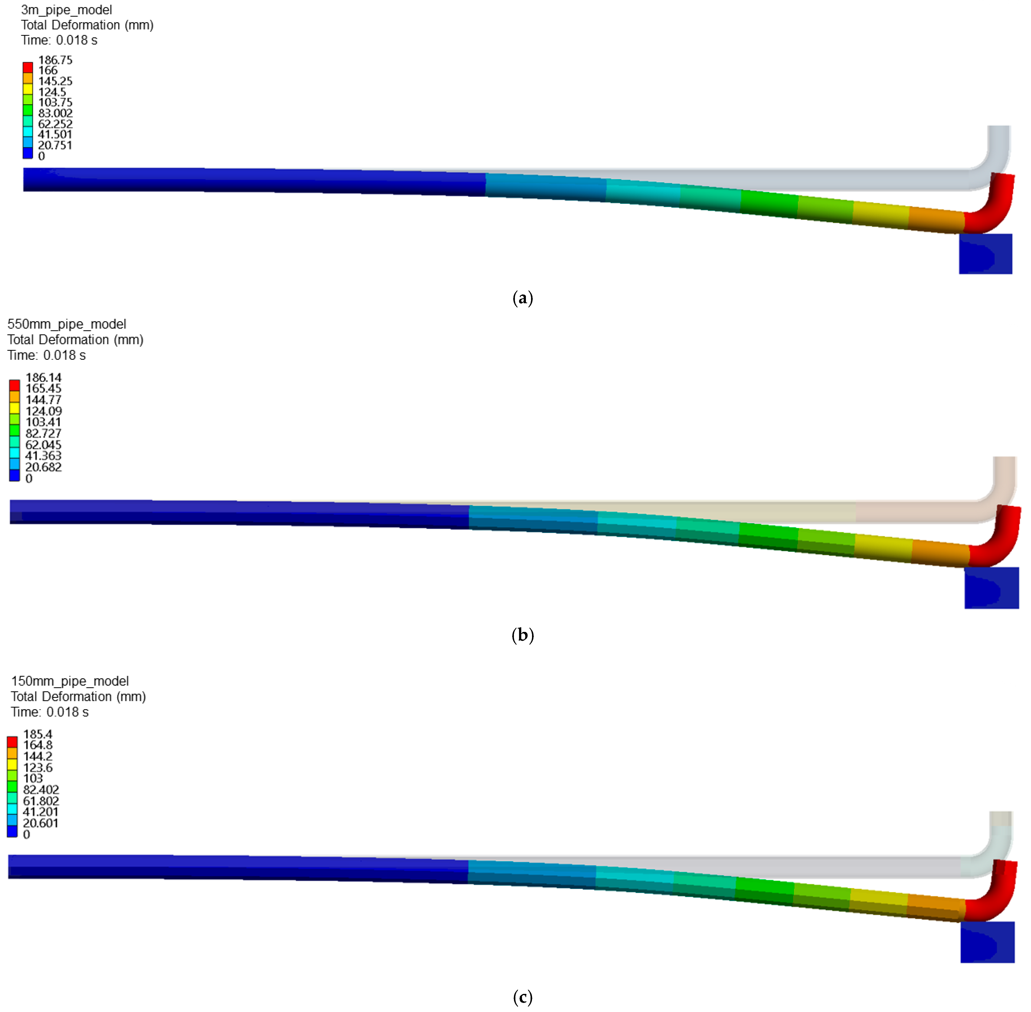
Fully 3D model (Ansys R2)	18	16.26
550 mm Solid Pipe model (Extended) (beam–solid formulation)	18	15.97
150 mm Solid Pipe model (Shortened) (beam–solid formulation)	18	16.37

, it is evident that all three models possess similarity in the time taken to impact after fluid flow initiation, while negligible differences can be observed in the impact velocity comparable with the experimental results [4]. The comparison of the models with the results of the ABAQUS-EPGEN and TEDEL codes are in close agreement with the impact time.

These results show that the simplified coupled models can be substituted for the solid models where the kink locations are being majorly considered to estimate the mechanical behaviour under impact conditions. All three models show similar deformable behaviour, as shown in Figure 12, even with the simplified approach of reducing the solid model to 5% of its original length. However, the fluid modeling parameters can be developed for the FSI models by taking into consideration the two-way FSI approach and solving under controlled water hammer conditions.

The comparison of the model parameters is shown in

Table 3. Structural response of the three models in the transient structural module.

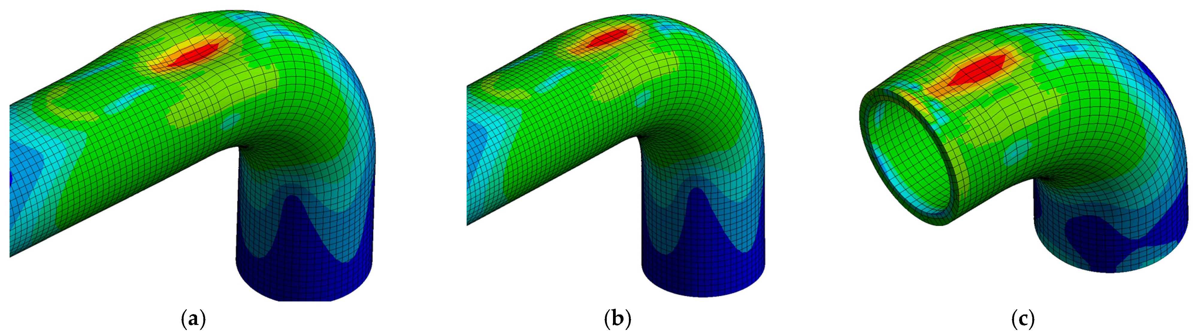
		Structural Pipe Models with 5 mm Element Size
		Fully 3D Model	550 mm Pipe Model	150 mm Pipe Model
Total displacement (mm)		186.75	186.14	185.4
Eq. von Mises stress (MPa)		487.49	488.19	492.32
Finite elements count	Total nodes	448,244	87,021	35,184
	Total elements	83,206	16,688	7149
Computational time (min)		111.8	15.9	6.6

and their independent displacement contours are shown in Figure 15a–c which predicts similar mechanical displacements for all three models, suggesting that a localized solid modeling technique can generate equal and optimal results with significant differences in their computational time and effort. The maximum values of total displacement and the equivalent von Mises stress are almost similar to the pipe-to-wall impact model for both the simplified model cases. However, the computational time is significantly reduced for the localized 150 mm model, which contains less than half the number of finite elements when compared to the 550 mm model, and all three models behave similarly under the dynamic structural conditions.

5. Discussion

This research was dedicated to analyzing the structural response due to fluid fast transients of the pipe models for varying localized 1D/3D coupled numerical models. A complete numerical three-dimensional model involves huge data with an increased computational time and expense which can be demanding in complex non-linear and dynamic structural problems. Hence, the localization of model strengthening and model simplification in the areas of non-interests is desired to reduce the computational expense overall. This research simulates a fully three-dimensional model and two locally simplified models coupled with 1D and 3D elements with varying lengths by estimating the model behavior under dynamic FSI conditions depicting the pipe whipping effect.

The phenomenon of water hammer effect was attempted using the finite volume approach in Ansys Fluent module with a water inlet pressure of 16.6 MPa in the three-dimensional fluid domain, and the corresponding structural response was simulated in the Transient Structural module of Ansys using the FSI approach. The structural models were developed with a coupled 1D/3D elements with localized solid elements in and near the impact zone. The displacement, stresses, and impact velocities were measured for both the extended and shortened 1D/3D models and compared with their modeling characteristics.

All three model predictions generated similar results in their mechanical behaviour under dynamics conditions with certain amounts of deviation in the equivalent stress plot for the 20 ms duration of the whipping phenomenon. It can be seen that the localized 3D model of 150 mm decreased the computational time significantly, even with a reduction in more than half the number of finite elements, as modelled with a 550 mm 3D model. These results help in understanding the structural behaviour of the simplified models and their necessity for use in dynamic simulations.

6. Conclusions

To validate the modeling of pipe whipping phenomenon based on fluid–structure interaction, the Ansys computational tool was used, utilizing both Fluent and Transient Structural modules coupled together. Two different simplified pipe geometries were modelled using a coupled 1D/3D modeling approach differentiating in their longitudinal length (550 mm and 150 mm) at the elbow region of the free end of the Aquitaine pipe model. An instantaneous break of high-pressure fluid at the inlet of the pipe was considered to model the pipe whipping effect using CFD computation. The relative pressure differences inside the walls of the pipe were coupled to the Transient Structural module of Ansys to predict the structural response of the model until impact on the neighboring wall. A fully 3D model was also solved under similar conditions and then compared to the simplified models for model verification.

The numerical results as predicted by the Ansys computational tool provided fair validation with the experimental results of the CEA pipe whipping tests on the structural behaviour under dynamic conditions. Both the extended and shortened models (550 mm and 150 mm) along with the fully 3D model provided good correlation with the experimental results on the velocity at impact with deviations in the impact time against the ABAQUS-EPGEN (V4.5) and TEDEL (CEASEMT-V1) codes which used specific beam formulations, which diminished certain structural parameters, like strain rate and crushing stiffness. The pipe models were then compared for the accuracy on structural response from geometrical variance. The displacement and stresses came into good agreement with all three models while the 150 mm model containing much fewer elements than the 550 mm model decreased the computational time by 55%.

Thus, the simplified 1D/3D coupled modeling approach by minimizing the area of the solid region by constricting it to the impact area with appropriate contact modeling at the junctures can be considered in the future for decreasing the computational time and the formulation of finite elements. This computational research can be applied to internal FSI problems involving dynamic response and structural non-linearity. Structural impact simulations can further be developed using beam–shell element formulation by prioritizing the contact models for localized coupling approaches and to estimate the various other mechanical characteristics, like strain rate and localized stiffness behavior.

References

- Guilbaud, D.; Blay, N.; Broc, D.; Chaudat, T.; Feau, C.; Sollogoub, P.; Wang, F.; Baj, F.; Bung, H.; Combescure, D.; et al. An Overview of Studies in Structural Mechanics; CEA-R-6113; 2006; Available online: https://inis.iaea.org/search/search.aspx?orig_q=RN:38045517 (accessed on 21 September 2023).
- Garcia, J.L.; Chouard, P.; Sermet, E. Experimental Studies of Pipe Impact on Rigid Restraints and Concrete Slabs. Nucl. Eng. Des. 1984, 77, 357–368. [Google Scholar] [CrossRef]
- Kulak, R.F.; Narvydas, E. Verification of the NEPTUNE Computer Code for Pipe Whip Analysis. In Proceedings of the SMiRT 16—16th International Conference on Structural Mechanics in Reactor Technology, Washington, DC, USA, 12–17 August 2001. [Google Scholar]
- Hsu, L.C.; Kuo, A.Y.; Tang, H.T. Nonlinear Analysis of Pipe Whip. In Proceedings of the SMiRT 8, Brussels, Belgium, 19–23 August 1985. F1 4/6. [Google Scholar]
- Potapov, S.; Galon, P. Modelling of Aquitaine II Pipe Whipping Test with the EUROPLEXUS Fast Dynamics Code. Nucl. Eng. Des. 2005, 235, 2045–2054. [Google Scholar] [CrossRef]
- Daude, F.; Galon, P.; Douillet-Grellier, T. 1D/3D Finite-Volume Coupling in Conjunction with Beam/Shell Elements Coupling for Fast Transients in Pipelines with Fluid–Structure Interaction. J. Fluids Struct. 2021, 101, 103219. [Google Scholar] [CrossRef]
- Everstine, G.C. Dynamic Analysis of Fluid-Filled Piping Systems Using Finite Element Techniques. J. Press. Vessel. Technol. 1986, 108, 57–61. [Google Scholar] [CrossRef]
- Ezkurra, M.; Ander Esnaola, J.; Martinez Agirre, M. Analysis of One-Way and Two-Way FSI Approaches to Characterise the Flow Regime and the Mechanical Behaviour during Closing Manoeuvring Operation of a Butterfly Valve; ALUHYDRO View Project Green Hydrogen Technologies: H2 Generation, Storage and Transformation View Project; World Academy of Science, Engineering and Technology: Istanbul, Turkey, 2018. [Google Scholar]
- Dahmane, M.; Boutchicha, D.; Adjlout, L. One-Way Fluid Structure Interaction of Pipe under Flow with Different Boundary Conditions. Mechanics 2017, 22, 495–503. [Google Scholar] [CrossRef]
- Cai, S.; Li, Q.; Liu, C.; Zhou, Y. Evaporation of R32/R152a Mixtures on the Pt Surface: A Molecular Dynamics Study. Int. J. Refrig. 2020, 113, 156–163. [Google Scholar] [CrossRef]
- Lema, M.; López Peña, F.; Buchlin, J.-M.; Rambaud, P.; Steelant, J. Analysis of Fluid Hammer Occurrence with Phase Change and Column Separation Due to Fast Valve Opening by Means of Flow Visualization. Exp. Therm. Fluid Sci. 2016, 79, 143–153. [Google Scholar] [CrossRef]
- Bergant, A.; Simpson, A.R.; Tijsseling, A.S. Water Hammer with Column Separation: A Historical Review. J. Fluids Struct. 2006, 22, 135–171. [Google Scholar] [CrossRef]
- Uspuras, E.; Kaliatka, A.; Dundulis, G. Analysis of Potential Waterhammer at the Ignalina NPP Using Thermal-Hydraulic and Structural Analysis Codes. In Proceedings of the Transactions of the 15th International Conference on Structural Mechanics in Reactor Technology (SMiRT-15), Seoul, Republic of Korea, 15–20 August 1999. [Google Scholar]
- Martins, N.M.C.; Soares, A.K.; Ramos, H.M.; Covas, D.I.C. CFD Modeling of Transient Flow in Pressurized Pipes. Comput. Fluids 2016, 126, 129–140. [Google Scholar] [CrossRef]
- Jha, P.N.; Zhang, J.; Dalton, C. Numerical Simulation of Laminar Water Hammer Flow in a Pipe with Varying Cross-Section. J. Appl. Water Eng. Res. 2018, 6, 228–235. [Google Scholar] [CrossRef]
- Sun, Z.; Liu, D.; Yuan, H.; Sun, Z.; Pan, W.; Zhang, Z.; Ma, B.; Jiang, Z. The Water Hammer in the Long-Distance Steam Supply Pipeline: A Computational Fluid Dynamics Simulation. Cogent Eng. 2022, 9, 2127472. [Google Scholar] [CrossRef]
- Zhang, X.; Cheng, Y.; Xia, L.; Yang, J. CFD Simulation of Reverse Water-Hammer Induced by Collapse of Draft-Tube Cavity in a Model Pump-Turbine during Runaway Process. IOP Conf. Ser. Earth Environ. Sci. 2016, 49, 052017. [Google Scholar] [CrossRef]
- Geng, J.; Yuan, X.; Li, D.; Du, G. Simulation of Cavitation Induced by Water Hammer. J. Hydrodyn. 2017, 29, 972–978. [Google Scholar] [CrossRef]
- Huang, Q.; Liu, Z.; Wang, L.; Ravi, S.; Young, J.; Lai, J.C.S.; Tian, F.-B. Streamline Penetration, Velocity Error, and Consequences of the Feedback Immersed Boundary Method. Phys. Fluids 2022, 34, 097101. [Google Scholar] [CrossRef]
- Blair, S.R.; Kwon, Y.W. Modeling of Fluid–Structure Interaction Using Lattice Boltzmann and Finite Element Methods. J. Press. Vessel. Technol. 2015, 137, 021302. [Google Scholar] [CrossRef]
- Mei, R.; Shyy, W.; Yu, D.; Li, F.; Luo, L.-S. Lattice Boltzmann Method for 3-D Flows with Curved Boundary; NASA Langley Research Center: Hampton, VA, USA, 2002. [Google Scholar]
- Xu, L.; Tian, F.-B.; Young, J.; Lai, J.C.S. A Novel Geometry-Adaptive Cartesian Grid Based Immersed Boundary–Lattice Boltzmann Method for Fluid–Structure Interactions at Moderate and High Reynolds Numbers. J. Comput. Phys. 2018, 375, 22–56. [Google Scholar] [CrossRef]
- Feng, T.; Zhang, D.; Song, P.; Tian, W.; Li, W.; Su, G.H.; Qiu, S. Numerical Research on Water Hammer Phenomenon of Parallel Pump-Valve System by Coupling FLUENT with RELAP5. Ann. Nucl. Energy 2017, 109, 318–326. [Google Scholar] [CrossRef]
- Tijsseling, A.S.; Bergant, A.; Ljubljana, L.E. Meshless Computation of Water Hammer. Scientific Bulletin of the “Politehnica”. In Proceedings of the 2nd IAHR International Meeting of the Workgroup on Cavitation and Dynamic Problems in Hydraulic Machinery and Systems, Timisoara, Romania, 24–26 October 2007; Volume 52. [Google Scholar]
- Kumar Patel, A. Experimental Study of Water Hammer Pressure in a Commercial Pipe. IOSR J. Mech. Civ. Eng. Spec. Issue–AETM 2016, 16, 16–21. [Google Scholar] [CrossRef]
- Riedelmeier, S.; Becker, S.; Schlücker, E. Identification of the Strength of Junction Coupling Effects in Water Hammer. J. Fluids Struct. 2017, 68, 224–244. [Google Scholar] [CrossRef]
- Aliabadi, H.K.; Ahmadi, A.; Keramat, A. Frequency Response of Water Hammer with Fluid-Structure Interaction in a Viscoelastic Pipe. Mech. Syst. Signal Process 2020, 144, 106848. [Google Scholar] [CrossRef]
- Zhang, L.; Tijsseling, A.S.; Vardy, A.E. FSI Analysis of Liquid-Filled Pipes. J. Sound Vib. 1999, 224, 69–99. [Google Scholar] [CrossRef]
- Zhang, Y.; Vairavamoorthy, K. Analysis of Transient Flow in Pipelines with Fluid-Structure Interaction Using Method of Lines. Int. J. Numer. Methods Eng. 2005, 63, 1446–1460. [Google Scholar] [CrossRef]
- Daude, F.; Galon, P. A Finite-Volume Approach for Compressible Single- and Two-Phase Flows in Flexible Pipelines with Fluid-Structure Interaction. J. Comput. Phys. 2018, 362, 375–408. [Google Scholar] [CrossRef]
- Martins, N.M.C.; Carriço, N.J.G.; Covas, D.I.C.; Ramos, H.M. Velocity-Distribution in Pressurized Pipe Flow Using CFD: Mesh Independence Analysis; 2014; ISBN 9789899647923. Available online: https://www.researchgate.net/profile/Nuno-Martins-14/publication/266259133_Velocity-Distribution_in_Pressurized_Pipe_Flow_using_CFD_Mesh_Independence_Analysis/links/542aeac80cf29bbc126a7a27/Velocity-Distribution-in-Pressurized-Pipe-Flow-using-CFD-Mesh-Independence-Analysis.pdf (accessed on 21 September 2023). [CrossRef]
- Knotek, S.; Schmelter, S.; Olbrich, M. Assessment of Different Parameters Used in Mesh Independence Studies in Two-Phase Slug Flow Simulations. Meas. Sens. 2021, 18, 100317. [Google Scholar] [CrossRef]
- Förster, C.; Wall, W.A.; Ramm, E. Artificial Added Mass Instabilities in Sequential Staggered Coupling of Nonlinear Structures and Incompressible Viscous Flows. Comput. Methods Appl. Mech. Eng. 2007, 196, 1278–1293. [Google Scholar] [CrossRef]
- Meduri, S.; Cremonesi, M.; Perego, U.; Bettinotti, O.; Kurkchubasche, A.; Oancea, V. A Partitioned Fully Explicit Lagrangian Finite Element Method for Highly Nonlinear Fluid-Structure Interaction Problems. Int. J. Numer. Methods Eng. 2018, 113, 43–64. [Google Scholar] [CrossRef]
- Chen, Y.; Zhao, C.; Guo, Q.; Zhou, J.; Feng, Y.; Xu, K. Fluid-Structure Interaction in a Pipeline Embedded in Concrete During Water Hammer. Front. Energy Res. 2022, 10, 956209. [Google Scholar] [CrossRef]
- Gnedin, N.Y.; Semenov, V.A.; Kravtsov, A.V. Enforcing the Courant–Friedrichs–Lewy Condition in Explicitly Conservative Local Time Stepping Schemes. J. Comput. Phys. 2018, 359, 93–105. [Google Scholar] [CrossRef]
- Aune, V.; Valsamos, G.; Casadei, F.; Langseth, M.; Børvik, T. Fluid-Structure Interaction Effects during the Dynamic Response of Clamped Thin Steel Plates Exposed to Blast Loading. Int. J. Mech. Sci. 2021, 195, 106263. [Google Scholar] [CrossRef]
- Aune, V.; Valsamos, G.; Casadei, F.; Langseth, M.; Børvik, T. Influence of Fluid-Structure Interaction Effects on the Ductile Fracture of Blast-Loaded Steel Plates. EPJ Web Conf. 2021, 250, 02019. [Google Scholar] [CrossRef]
- Hu, J.; Wang, X.; Li, Y.; Wen, X.; Wu, Y.; Huang, Y. Investigation of Whipping Effect on High Energy Pipe Based on Fluid-Structure Interaction Method. Int. J. Impact Eng. 2023, 173, 104463. [Google Scholar] [CrossRef]
- Everstine, G.C. Transient Fluid-Structure Interaction Using Finite Elements. In Proceedings of the Fluid-Structure Interaction and Structural Mechanics—Joint ASME/JSME Pressure Vessels and Piping Conference, Honolulu, HI, USA, 23–27 July 1995; pp. 77–84. [Google Scholar]
- Andersson, C.; Ahl, D. Fluid Structure Interaction; Halmstad University: Halmstad, Sweden, 2011. [Google Scholar]
- Guo, Q.; Zhou, J.; Li, Y.; Guan, X.; Liu, D.; Zhang, J. Fluid-Structure Interaction Response of a Water Conveyance System with a Surge Chamber during Water Hammer. Water 2020, 12, 1025. [Google Scholar] [CrossRef]
- Sai, V.; Sudula, P. Bilinear Isotropic and Bilinear Kinematic Hardening of AZ31 Magnesium Alloy. Int. J. Adv. Res. Eng. Technol. 2020, 11, 518–531. [Google Scholar]