Article

High-Fidelity Drone Simulation with Depth Camera Noise and Improved Air Drag Force Models

Department of Mechanical Engineering, Sungkyunkwan University, Suwon 16419, Republic of Korea
*
Authors to whom correspondence should be addressed.
Appl. Sci. 2023, 13(19), 10631; https://doi.org/10.3390/app131910631
Submission received: 8 August 2023 / Revised: 18 September 2023 / Accepted: 19 September 2023 / Published: 24 September 2023
(This article belongs to the Special Issue Advanced Robotics and Mechatronics)

Abstract

:
Drone simulations offer a safe environment for collecting data and testing algorithms. However, the depth camera sensor in the simulation provides exact depth values without error, which can result in variations in algorithm behavior, especially in the case of SLAM, when transitioning to real-world environments. The aerodynamic model in the simulation also differs from reality, leading to larger errors in drag force calculations at high speeds. This disparity between simulation and real-world conditions poses challenges when attempting to transfer high-speed drone algorithms developed in the simulated environment to actual operational settings. In this paper, we propose a more realistic simulation by implementing a novel depth camera noise model and an improved aerodynamic drag force model. Through experimental validation, we demonstrate the suitability of our models for simulating real-depth cameras and air drag forces. Our depth camera noise model can replicate the values of a real depth camera sensor with a coefficient of determination ( R 2 ) value of 0.62, and our air drag force model improves accuracy by 51% compared to the Airsim simulation air drag force model in outdoor flying experiments at 10 m/s.

1. Introduction

Autonomous drones, also known as unmanned aerial vehicles (UAVs), hold tremendous potential across various domains due to their high-speed flight capabilities and capacity to perform missions without human intervention [1]. These applications include reconnaissance [2,3], security [4], transportation [5], agriculture [6], construction [7,8], and mapping [9,10]. However, deploying and testing autonomous drones in real-world environments poses challenges, including safety concerns [11,12], as well as the costs and time required. Consequently, many studies on autonomous drones opt for simulation-based experimentation over real-world scenarios [13].
Among numerous drone simulators, Airsim stands as a widely adopted environment for autonomous drone testing, offering comprehensive components such as environment models, vehicle models, physics engines, sensor models, and a rendering interface. It harnesses the high-speed processing capabilities of the NVIDIA PhysX engine, performing kinematic computations at 1000 Hz using state values, including position, orientation, linear velocity, linear acceleration, angular velocity, and angular acceleration [14]. Airsim can also simulate the standard temperature and pressure using the 1976 U.S. standard atmosphere model. As seen in Figure 1, Unreal Engine, known for its exceptional rendering quality, powers the simulation environment. Unreal Engine’s robust collision detection system provides detailed information about collision impact positions, impact normals, and penetration depths. This synergy enables Airsim to simulate camera sensors with high-quality rendering when coupled with Unreal Engine. Regarding sensor models, Airsim features realistic representations of a barometer (MEAS MS5611-01BA), magnetometer (Honeywell HMC5883), and IMU (InvenSense MPU 6000), complete with Gaussian noise modeling. Additionally, Airsim includes GPS models with simulated vertical and horizontal error, along with a 200 ms latency.
Although Airsim with Unreal Engine simulator has many advantages, it still has some disadvantages that need to be improved. In fact, for drones, the high-resolution rendering does not replicate the sensing and control in the same way between a real-world environment and in a simulation environment [15,16]. Compared to high-resolution rendering, the accurate implementation of depth camera and air drag force models is more important to make the simulation environment close to the real-life environment [17]. However, those models in Airsim simulation are unrealistic for accurately evaluating the control and estimation algorithms of a drone flight [18,19]. Specifically, the depth camera model is overly idealistic in the simulation since it provides the exact value without any errors [20]. In contrast, the aerodynamic model is too simplified, so the external force caused by air drag when the drone flies is unrealistic [21]. As a result, the algorithms for filtering the noise from the depth sensor [22], one of the most common sensors in drones to sense the surrounding environments [23], which are developed to test the drone in a real-world environment, cannot be adequately verified through simulations. The control algorithms tested in simulations, which aim to counter external forces like air drag, can lead to significant issues when applied in real-world scenarios. Therefore, in order to align the performance of autonomous drone algorithms developed in simulations with real-world operation, enhancements to the simulation are required. These enhancements should include a more realistic depth camera sensor and a dynamic air drag force model.
In this paper, our objective is to enhance the realism and accuracy of the drone simulation environment in Airsim with Unreal Engine. We propose two novel models: one for stereo IR depth camera noise and the other for air drag force, known as the rotor drag force model. As previously mentioned, Airsim lacks a depth camera noise model, which we address by introducing our own. In addition to considering noises caused by distance, as proposed in [24], we contribute to depth camera noise modeling by also accounting for noises caused by the materials of detected objects. This addition is significant as it has been demonstrated to have a substantial impact on depth camera noise [25]. Regarding the aerodynamic drag model, while Airsim currently uses only the velocity and rotation matrix to calculate the aerodynamic drag force [26], we enhance the modeling by incorporating thrust values. This enhancement has shown a substantial improvement in performance compared to the embedded model in Airsim. Furthermore, in addition to proposing these models, to the best of our knowledge, we are the first to implement these improved models in a drone simulator such as Airsim. This implementation is expected to make a significant contribution to drone research by providing a more effective platform for testing drone algorithms and training reinforcement learning methods.
Specifically, the depth noise is modeled as Gaussian noise. To identify and verify the parameters of the depth camera noise model, depth measurements were collected using the Intel RealSense D435 camera at distances ranging from 0.5 m to 8 m and on various materials. Additionally, simulations and experiments were conducted at various flight speeds to compare the accuracy of the proposed drag force model with the embedded model in Airsim. Experimental results demonstrated that the depth camera model becomes more accurate and realistic with varying distances and materials. Furthermore, the proposed drag force model was shown to reduce acceleration errors by up to 51 % when compared to the Airsim-provided model during high-speed flights at 10 m/s in a real flight scenario.
In short, our contribution includes:
  • Development of an improved model of the depth model by embedding a Gaussian noise model, which was verified through experiments, into the depth camera model. This modification makes the depth camera model more accurate and realistic across various distances and materials.
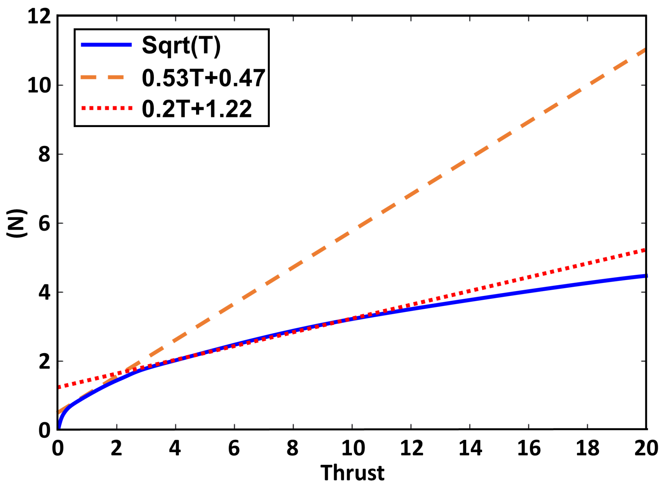
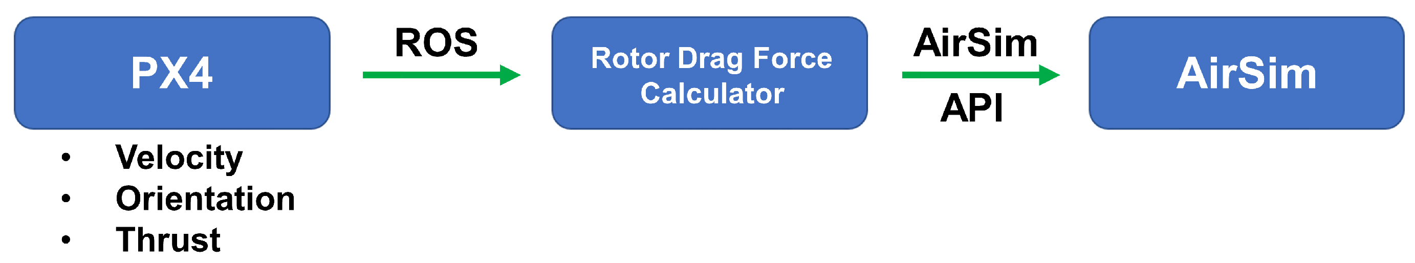
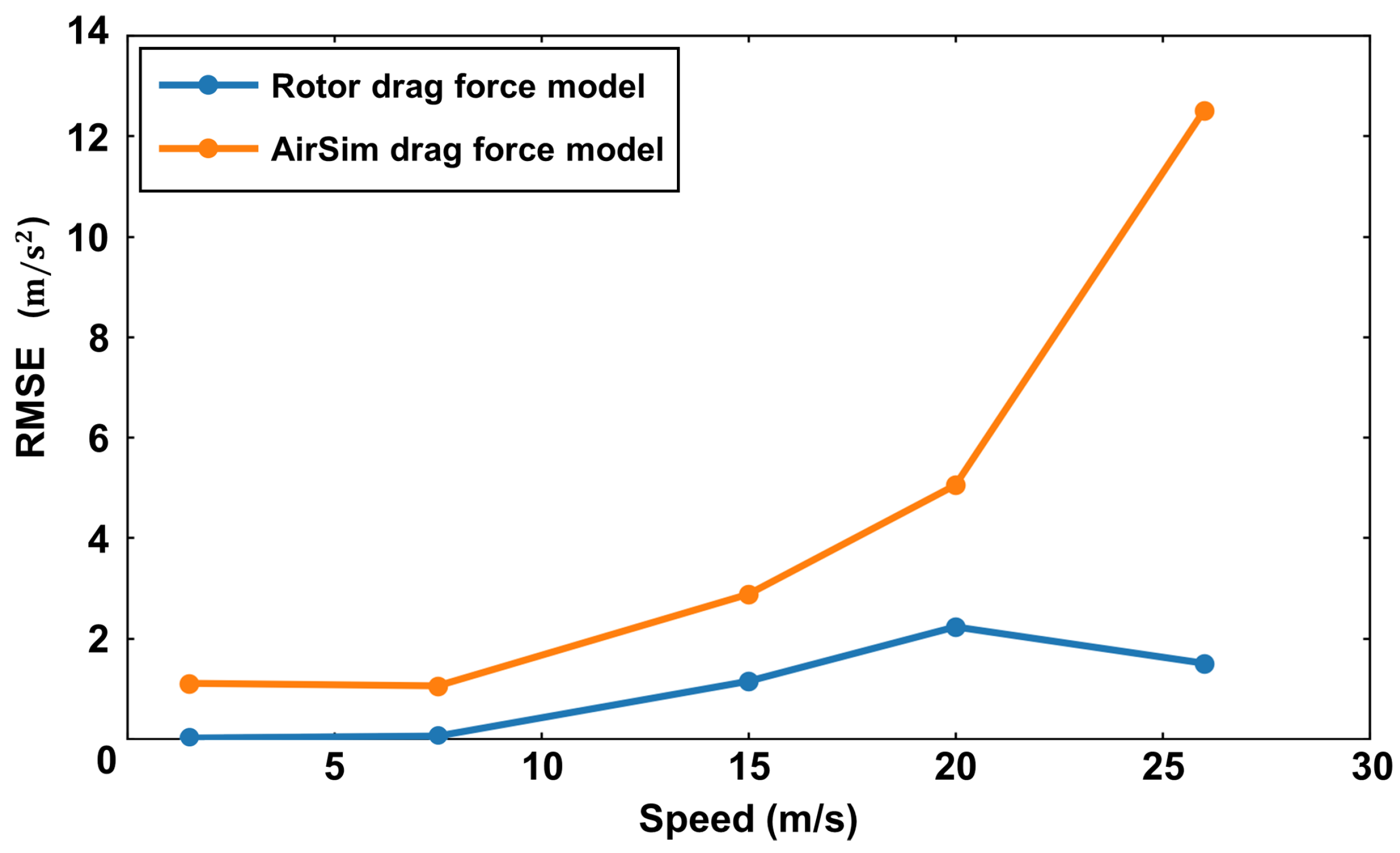
  • Development of an improved rotor air drag force model. By including thrust values in addition to drone velocity and rotation, we create a force model that more accurately represents real-world air drag forces.
  • Providing an improved simulation environment that is more reliable for testing the real-world behavior of autonomous drones compared with the existing Airsim simulator, especially in high-speed drone flight experiments.
This paper is composed as follows. Section 2 presents depth camera modeling with simulation implementation. Section 3 shows rotor drag force model implementation with test results, and finally, Section 4 provides a conclusion.

2. Depth Camera Modeling and Implementation

In this section, we briefly introduce the stereo IR depth camera and propose the Stereo IR depth camera noise model. For depth cameras, noises might originate from various factors. Primary sources include the distance from the camera to the object. Lateral noise, lighting conditions, and the materials of the detecting objects also play significant roles in the noise profile [25]. For the active sensor D435, there is negligible lateral noise [25]. In this paper, we focus particularly on two dominant noise sources: the distance from the camera to the object and the noises originating from the materials of the detecting objects. The noise model’s parameters will be identified and verified through experiments involving various materials and distances. The depth camera model will be implemented in the simulation and compared to the real camera values using the coefficient of determination.

2.1. Stereo IR Depth Camera

A Stereo IR depth camera comprises an IR projector and two IR cameras. The IR projector emits a dot pattern on the front of the camera, and two IR cameras capture the pattern. As in Figure 2a, the Intel realsense D435 camera has two IR cameras and an IR projector. When detecting objects, the projected dot pattern from the IR projector is reflected off the measured materials and detected by the IR cameras. Because of the distance between the two cameras, the position of the pattern measured on the two cameras is different. As in Figure 2b, The depth between the camera and an object can be calculated using the disparity value from two camera measurements. The equation is written as follows [27]:
b Z = ( b + x L ) x R Z f
Z = b · f x R x L
The Z is the depth value, x R is the measurement of the right camera, x L is the measurement of the left camera, b is the distance between the two cameras, and f is the focal length of the camera as shown in Figure 2b.
When the detecting object is close to the depth camera, the disparity value is high, and an accurate depth value can be calculated [28]. Conversely, when the detecting object is far from the depth camera, the error of the calculated depth is increased due to a small disparity value [29]. Moreover, since different materials have different surface structures, they will affect the visibility of the pattern leading to variations in depth error.

2.2. Experimental Setup

To investigate the impact of distance and material of the detecting object on the depth error, indoor experiments using Intel Realsense D435 depth camera have been conducted to collect the depth values with 3 different materials. Our experimental setup is similar to the setup proposed in [30]. While we also vary the distance in the experiment, the significant difference between our setup and the setup in [30] is that we adopt different wall materials (plastic, cement, formboard) to analyze their effects on the depth noise. The experimental setup can be seen in Figure 3.
Before conducting the experiment, we calibrated the D435 depth camera by utilizing Intel’s Dynamic Calibration tool, following the connection of the D435 camera to a laptop via a USB3 cable [30]. During the calibration process, the program analyzes all depth values within the full field of view. In addition, we assessed the depth quality using the depth quality tool provided by the Intel RealSense SDK [30,31]. To confirm depth quality, the camera needed to have more than 50 % valid depth points, without the requirement for a flat or perpendicular surface. Following calibration, we employed the Realsense ROS program to publish the sensor data from the depth camera to our laptop. For each material, the distance of the depth camera to the wall was manually set from 0.5 m to 8 m at 1 cm step (751 camera positions in total) using a roller. The distance was measured with the accuracy of 1 mm. After calibrating the camera’s position, we check again if the camera is perpendicular to the wall using the depth image. Using the real-time data streaming from a ROS topic, we divided the depth image into four sections; the perpendicular condition is then guaranteed if the average depth values of all sections were the same. A depth image with the size of 460 × 320 pixels was obtained at each distance. For 751 camera positions, 751 corresponding depth images can be obtained for each material.

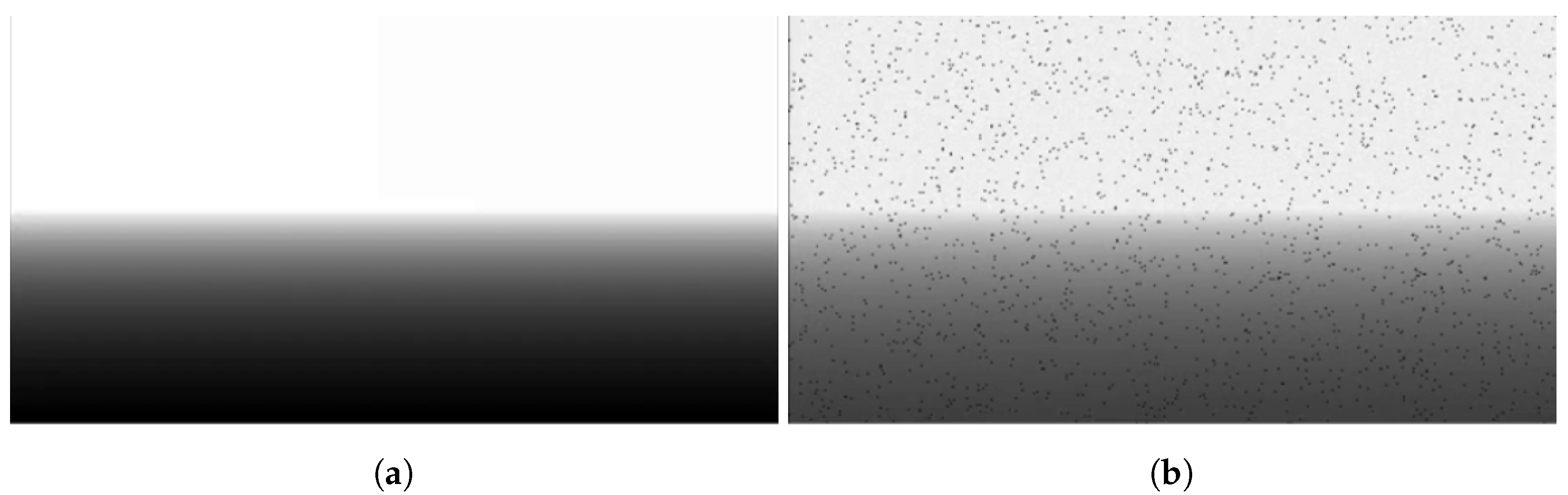
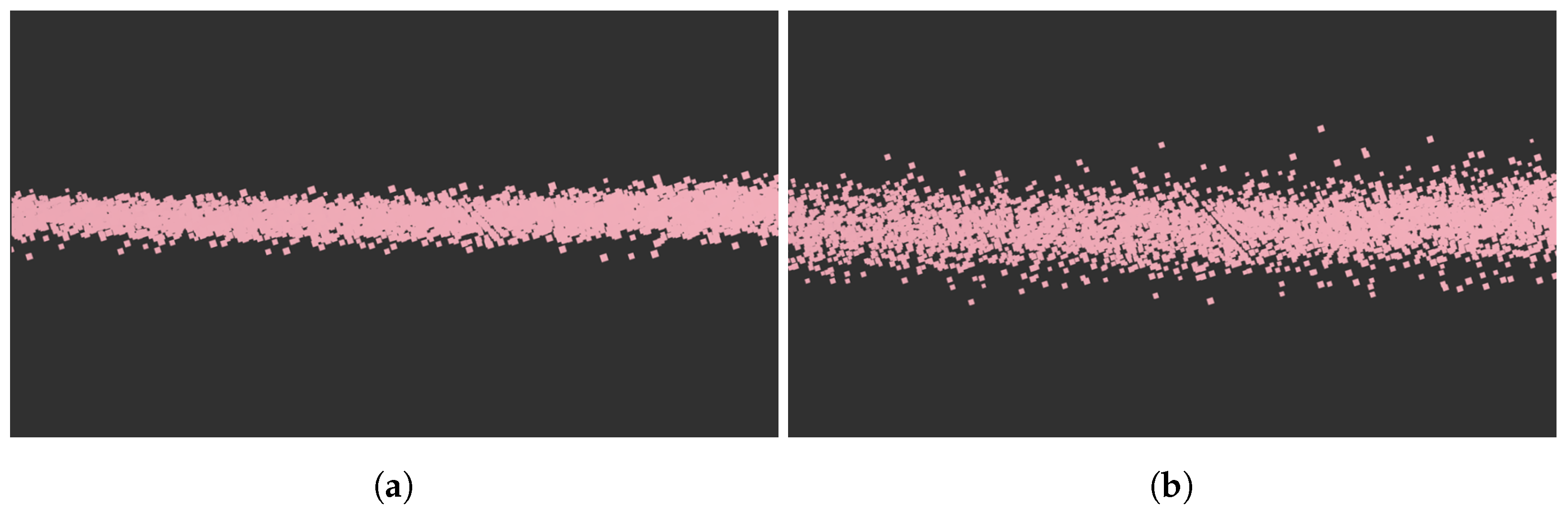
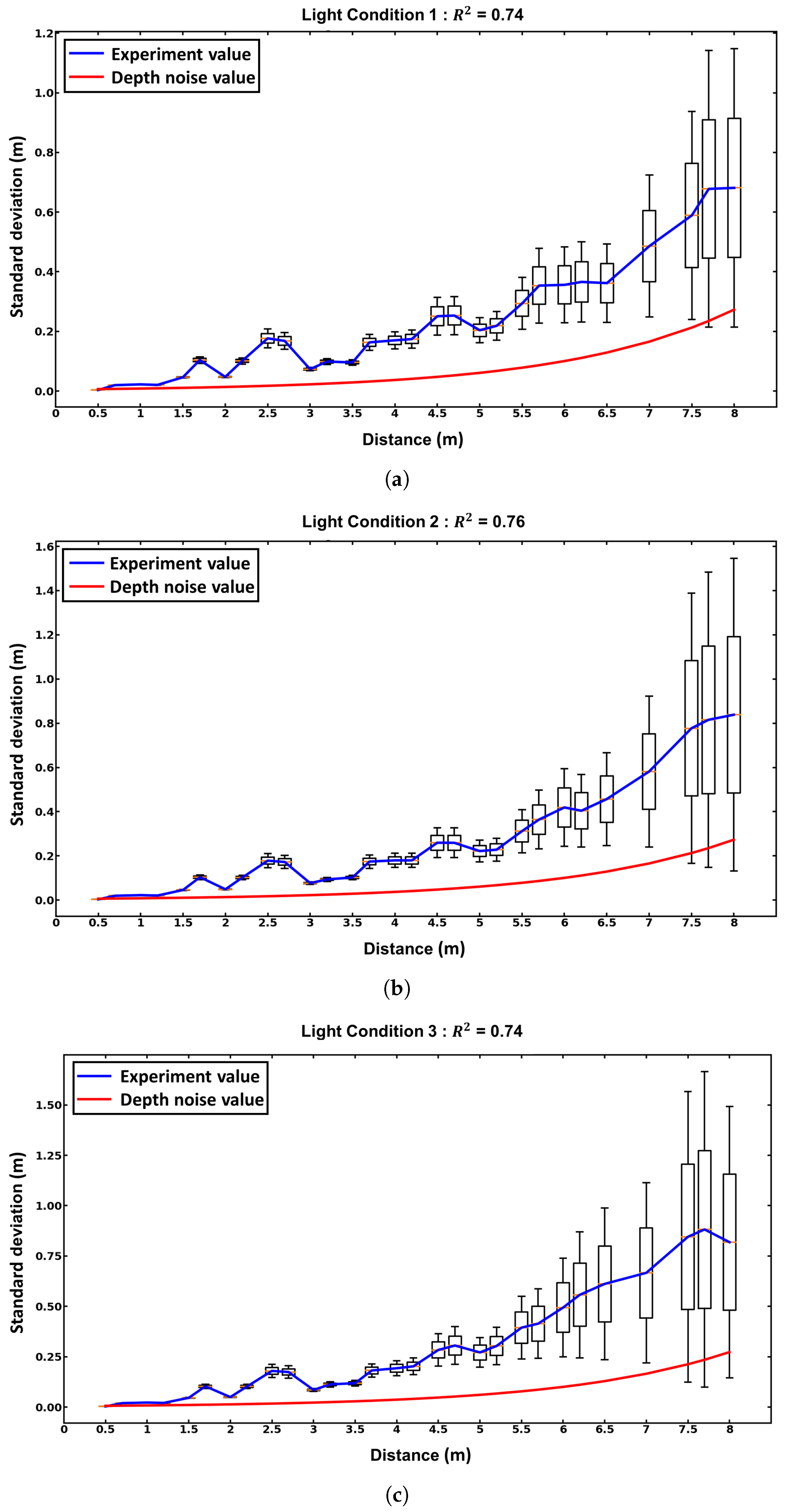
2.3. Depth Noise Modeling

It was pointed out that the depth noise from Intel Realsense D435 can be modeled as a Gaussian model [25,30]. The standard deviation of the noise model is calculated based on the depth data obtained in Section 2.2 as follows. Since the true distance value is known, the depth error at each pixel can be calculated as in Equation (3).
D e p t h e r r o r = D e p t h m e a s u r e d D e p t h t r u e
The standard deviation value of the 460 × 320 D e p t h e r r o r values can then be computed. Figure 4 illustrates the calculated standard deviation values of the depth error for all three materials. It was observed that the standard deviation values for each material increase exponentially with distance. This trend is exhibited by all three materials, albeit with different specific patterns. Based on this observation, multiple candidate functions, including exponential functions and other polynomial functions, were tested to find the best fit for the data. The exponential function model in Equation (4) was ultimately selected because it yielded the smallest Root Mean Square Error (RMSE) values.
s t d n o i s e = 0.005 e m × d
where s t d n o i s e is the standard deviation of the depth error, m is the material value with the unit of 1/m, d is the distance value with the unit of meter, and 0.005 is the fitting coefficient with the unit of meter.
The graph depicted in Figure 4 illustrates how the standard deviation of the depth value varies with different material values. Additionally, there is another type of error known as the fill-rate error, which arises when the depth camera cannot calculate the depth value for certain pixels due to the absence of a detectable dot pattern. These pixels are assigned a depth value of 0, and this error occurs randomly in 1 % of the depth camera pixels [32], as demonstrated in Figure 5. This fill-rate error is simulated by setting 1 % of the depth values to 0.

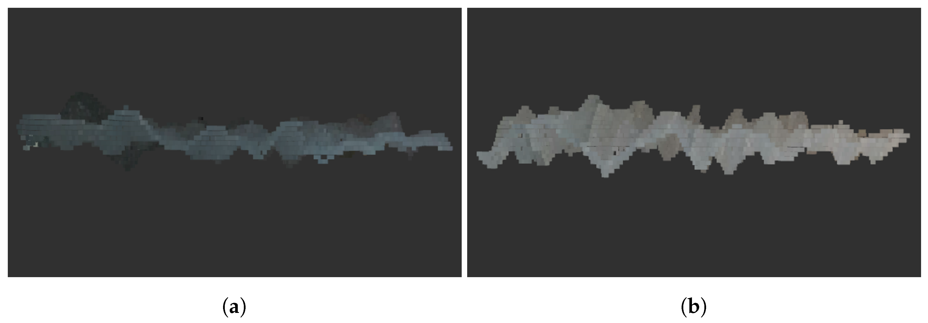
2.4. Simulation Implementation and Results

The depth camera model is implemented in the Airsim simulation to provide realistic depth camera functionality for drone simulations. As shown in Figure 6, the depth camera model (Equation (4)) generates a noise model based on the simulated depth value and subsequently applies it to the simulated depth value. In our work, we conducted simulations with a MSI laptop (Taipei, Taiwan) equipped with the following specifications: Intel i7-10750H processor, 16 GB DDR4 RAM, and an NVIDIA GeForce GTX 1660 Ti (laptop version). The simulation is run on Ubuntu 18.04 with ROS melodic version, Unreal Engine 4, Airsim, and PX4 programs [33]. Unreal Engine 4 was responsible for visualization of the simulation and enabled the creation of simulation environments with obstacles. On the other hand, PX4, an open-source drone control program, provided simulated internal sensors such as IMU and barometer [34,35]. Airsim links PX4 to Unreal Engine 4 and allows for the attachment of GPS, RGB camera, and depth camera to the simulated drone [26], as well as the ability to perform collision detection and map-scanning. When a control command is input into PX4, the control value is calculated, and the simulated drone begins to move [35]. The simulated drone’s position, velocity, and rotation are calculated in Airsim and visualized in Unreal Engine 4. Figure 5a illustrates that all pixels of the depth camera from the simulation have true depth values, while Figure 5b demonstrates the implementation of the fill-rate error in the simulation. Figure 6 provides an overview of the implementation of our depth camera noise model in simulation. We subscribe to the depth camera topic from Airsim to obtain depth information for the camera depth noise model. This information is used in our ROS package to compute Gaussian noise, following Equation (4). Subsequently, we publish the resulting noise values back to Airsim through another topic. The depth noise calculation at each pixel includes 2 multiplications and 1 exponential calculation. Its required calculation time depends on the processor’s capabilities. The complexity of the algorithm is then O ( n ) , where n is the number of depth points. Using our hardware setup, it takes approximately 0.0121 s to calculate the depth noise data for 460 × 320 pixels. The depth camera noise topic is then published back to Airsim at a rate of about 30 Hz, enabling real-time usage.
Figure 7a,b demonstrate how the depth value appears as a pointcloud when the material value is altered, causing the simulated measurement of a wall to appear thicker due to increased noise. To further evaluate our model, the coefficient of determination ( R 2 ) value was calculated between two standard deviation data sets for each material. One set is the standard deviation values calculated from a real environment using Intel Realsense D435 depth camera, while the other set is standard deviation values calculated from simulation using our depth camera model. Each set has 751 values as described in Section 2.2. R 2 values are shown in Table 1. The average coefficient of determination ( R 2 ) value is 0.6204, indicating that the depth camera noise model can accurately simulate different noise levels for different materials. However, it is important to note that the model errors tend to increase with distance. It is observed that the model performs optimally in the distance range from 0.5 m to 3 m (ideal range for D435 [36]) with an average R 2 of 0.92 for all materials (0.89 for plastic walls). In the range from 0.5 m to 6 m (the maximum range for drones), those values decrease to 0.73 and 0.5948, respectively.
The realism of our simulator can be visually verified as seen in Figure 7, Figure 8 and Figure 9. In Figure 7 and Figure 8, the depth data obtained from the real wall with different materials closely resemble the simulation depth data generated using the depth camera noise model. As shown in Figure 9, the depth camera noise model exhibits larger noise levels with increasing distance. To validate the proposed model, we conducted another indoor experiment using a Realsense D435 depth camera. The camera was stationary, capturing static objects from a perpendicular angle, as described in the experimental setup Section 2.2. For this experiment, we used a different cement wall than the one described in Section 2.2. The experimental setup remained consistent with the previous section. To vary the lighting conditions in real-world experiments, we utilized different LED lights (3000 Lumens, Z-9020M (Nanjing, China)). Light density was measured using a cellphone, and the recorded light density represented the average value measured in the testing area when the cellphone camera was directed from the wall towards the Realsense camera in a perpendicular direction. Three different light conditions were observed: 160 Lux, 230 Lux, and 300 Lux, all falling within the typical range of indoor lighting conditions [37]. It is worth noting that the light condition can be easily adjusted in the simulator.
The distance between the depth camera and the wall was manually adjusted from 0.5 m to 8 m, resulting in a total of 29 camera positions, using a roller. At each distance, we captured five depth images, each with a size of 460 × 320 pixels. The standard deviation values of the depth errors and their deviations can then be achieved. Using the depth camera model with noise for a cement wall (material value 0.5 1/m) obtained in Section 2.3, the comparison between the real standard deviations of the depth errors and the simulated standard deviations of the depth using our depth noise model for cement walls is shown in Figure 10. It is observed from Figure 10 that the average value of R 2 is 0.74 for three light conditions, validating the accuracy of our depth noise model. Furthermore, it is also observed that the noise model is not affected by the lighting condition under 300 Lux. Similar results were also observed with the same depth camera D435 tested under different lighting conditions under 540 Lux, but at shorter distances (1 m, 1.5 m) [38].
It was shown that incorporating a noise model results in better performance in SLAM and reconstruction algorithms [38], object recognition [39], segmentation [40], 3D reconstruction [41], and camera tracking [42]. Our depth noise camera model for those applications will be validated in our future work.

3. Rotor Drag Force Model Implementation

This section presents the development of the model for rotor air drag force. As our improved model is based on the embedded model in Airsim, we will first provide an overview of the Airsim drag force model, followed by an introduction to our proposed rotor drag force model in Section 3.1.
The process to verify our aerodynamic drag model is as follows. First, thrust experiments will be carried out to find the relationship between thrust and PWM inputs sent from Pixhawk (high-level controller) to the ESC (electronic speed controllers), as presented in Section 3.2.1. Because drag force cannot be measured directly, we will verify the model indirectly by comparing the calculated acceleration, which is the resulting acceleration caused by the thrust and drag force, and the measured acceleration of the drone, which is obtained using IMU and GPS sensors, as in Section 3.2.2. Both models are compared through both simulation and outdoor experimental tests at different speeds.

3.1. Rotor Drag Force Model
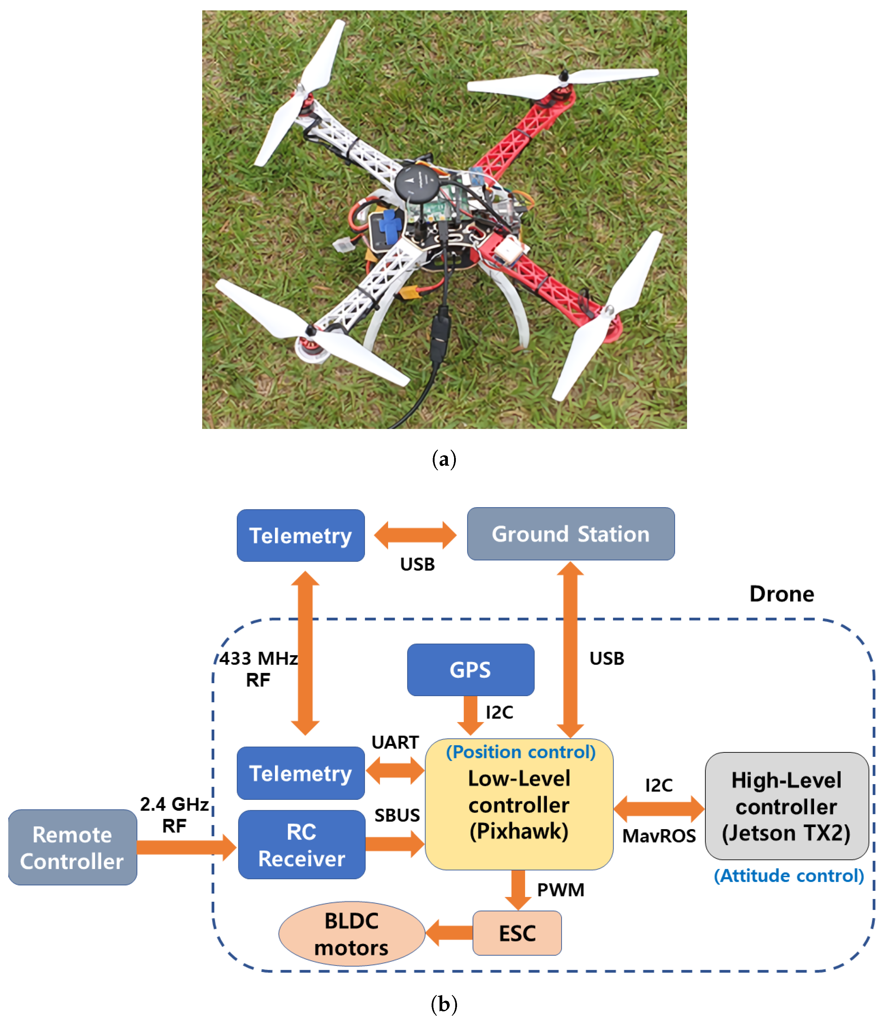
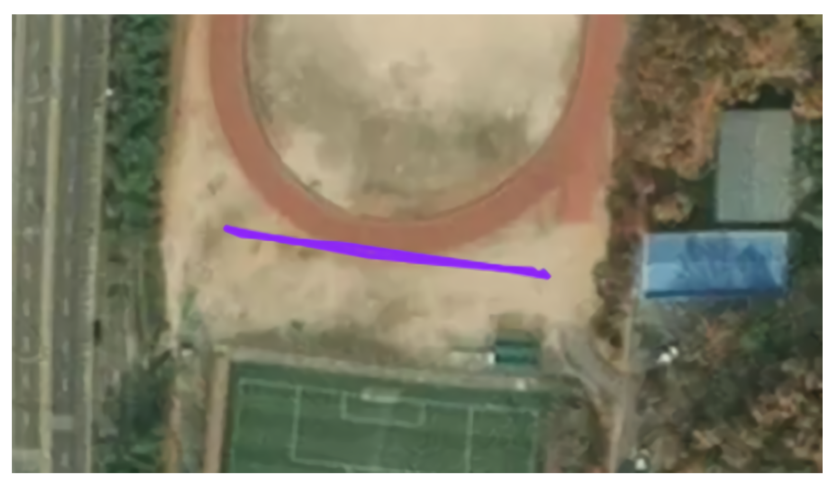
The air drag force model calculates the air friction in simulation. In Gazebo and Airsim simulator, the air drag force model [43] is implemented using the equation below.
F a = D R T V
where F a is the air drag force, D is the coefficient matrix, R is the rotation matrix of a drone, and V is the velocity of a drone. However, Equation (5) is too simplified for high-speed drone flight. To accurately simulate high-speed drone flight, we calculate more realistic aerodynamic forces by considering the forces acting on the drone’s rotor. The following equation demonstrates how air drag force acts on one rotor [44]:
F a i = T i c d 1 π e 3 V a i
where T i is the thrust generated by rotor i, V a i is relative air velocity expressed in the body frame, π e 3 = I e 3 e 3 , and e 3 is 0 0 1 . Due to T i in Equation (6), the rotor drag force does not satisfy differential flatness [45]. As shown in Figure 11, to satisfy differential flatness, T is linearized as below.
T i k T i + b , k , b > 0
where k and b are coefficients. Using the approximation in Equation (7), we can write Equation (6) as below:
F a i = k T i + b c d 1 π e 3 V a i
Since there are four rotors in a quadrotor, and the total air drag force can be expressed as follows.
F a = i = 1 4 F a i = i = 1 4 k T i + b c d 1 π e 3 V a i
where F a is the total air drag force acting on the quadrotor. The position vector of each rotor, represented as d i , is a combination of the horizontal position vector d ( x , y , i ) and the vertical position vector d ( z , i ) . By incorporating this information, Equation (9) can be expressed in the following form:
F a = i = 1 4 F a i = i = 1 4 k T i + b c d 1 π e 3 ( R T V a + ω × ( d i ) )
F a = i = 1 4 F a i = i = 1 4 k T i + b c d 1 π e 3 ( R T V a + ω × ( d x , y , i + d z , i ) )
where ω is angular velocity of quadrotor. It is common practice to place rotors symmetrically around the center of gravity and at the same height. This arrangement implies the use of an even number of rotors. According to [46], the effect of the wind, with speeds below 4 m/s, on the drone’s position can be considered negligible. In our experiments, the wind speed was consistently below 4 m/s, so we assumed there was no wind. Therefore, Equation (11) can be simplified as below:
F a = k T + b c d 1 π e 3 v k c d 1 π e 3 n / 2 i = 1 ( T i T i + n / 2 ) ( ω × d x , y , i )
where v is the quadrotor’s velocity. Since the thrust difference is primarily used to adjust the thrust vector when there is a change in the trajectory direction, it is assumed to be significantly smaller compared to the total thrust, which is responsible for hovering and following the trajectory. Equation (12) can then be rewritten as below:
F a = k T + b c d 1 π e 3 v
As shown in Figure 12, to implement rotor drag force in Airsim simulation, PX4 and Airsim program are used. The PX4 program subscribes to thrust, rotation, velocity topics published from Airsim. And we use the information from the topics to calculate the air drag force in our air drag force ROS package following Equation (13). The calculated result is then published back to the Aisim through another air drag force topic. Since the rotor drag force model involves only 21 basic calculations (multiplications and addition) as in Equation (13), it typically executed nearly instantly on current processors. With our hardware setup, the model takes only 4.36 × 10 6 s, making it suitable for real-time applications.

3.2. Experiments

To validate the drag force model, we conducted both simulated and real experiments using the F450 quadrotor equipped with a Sunnysky V3508 700 Kv BLDC motor (Shenzhen, China) and an 11 × 4.7 inch propeller, as shown in Figure 13a. Due to its simple structure and relatively small surface area, the drag force generated by the rotor is significant in comparison to the drag force originating from other parts of the drone, such as the drag force caused by the frame’s surface area. As shown in Figure 13b, the drone’s system architecture comprises an Nvidia Jetson TX2 with a J120 carrier board serving as the high-level controller and a Pixhawk2 as the low-level controller. The drone can operate in either manual mode or auto-pilot mode. In manual mode, commands are transmitted from a remote controller (RadioLink T8FB (Shenzhen, China)) to a remote controller receiver via 2.4 GHz radio communication. The receiver then relays signals to the low-level controller using the SBUS protocol. In auto-pilot mode, as depicted in Figure 13b, the drone’s position and speed are controlled by the high-level controller (Nvidia Jetson TX2 (Taipei, Taiwan)). The high-level controller subsequently sends commands to the Pixhawk using the MavROS package. In both modes, the Pixhawk manages the drone’s target attitude values, sending Pulse Width Modulation (PWM) values to the electronic speed controllers (ESCs) responsible for controlling the drone’s rotors. Flight data, including PWM signals sent to ESCs and the drone’s position, can be transmitted from the low-level controller to a ground station through telemetry using radio communication at 433 MHz or via a USB connection. The experiment utilized an Ubuntu 18.04 operating system, ROS Melodic, Mavlink, ROS, and PX4 programs. The IMU employed in flight experiments was integrated into the Pixhawk module, and a GPS device (CubePilot HERE2 M8N GPS (Xiamen, China)) was directly connected to the Pixhawk.

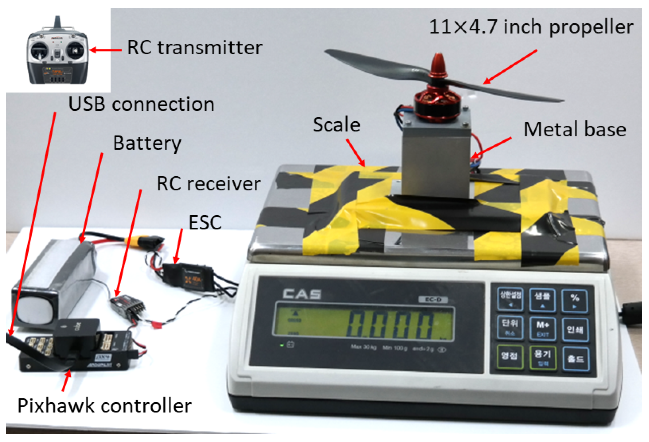
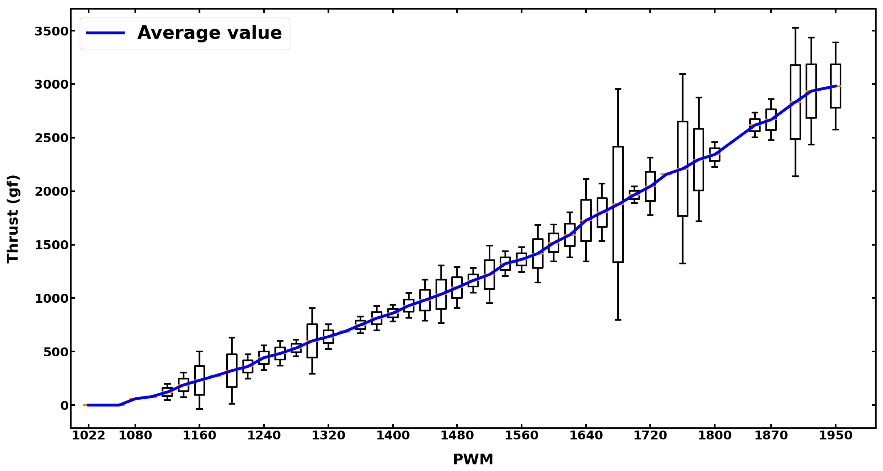
3.2.1. Thrust Experiments

To calculate the drag force in our model, the thrust value of the rotor is needed. Therefore, experiments have been conducted to determine the relationship between the PWM signals sent from Pixhawk to the ESC and the thrust produced by the rotor. The experimental setup can be seen in Figure 14. We used a Sunnysky V3508 700 Kv BLDC motor (Shenzhen, China) with an 11 × 4.7 inch propeller, the same as what was used in our drone. This motor was attached to a metal base fixed to a scale using tape. A 14.8 V battery powered the ESC. Throttle commands to adjust the rotor speed were sent from a remote control (RC) transmitter to an RC receiver, which then transmitted corresponding PWM signals to the electronic speed controller (ESC) responsible for regulating the rotor’s speed. We monitored the PWM values on a notebook through a ROS topic, received directly from the Pixhawk controller via USB connection. During experiments, we manually adjusted the remote controller to vary the PWM values from 1000 to 1950 in steps of approximately 20. We recorded thrust values displayed on the scale’s screen with a 1 g resolution. For each PWM value, we recorded five thrust values over 5 s, with measurements taken every 1 s. The test results are presented in Figure 15.

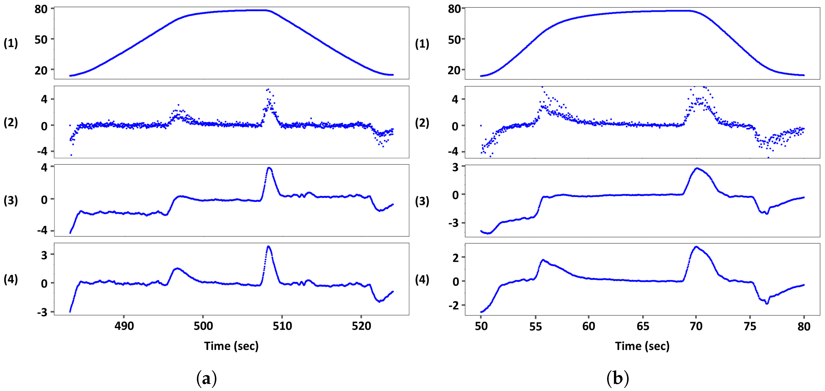
3.2.2. Rotor Drag Force Experiments

To validate our model, simulated experiments in an indoor environment at five different speeds of 1.5 m/s, 7.5 m/s, and 26 m/s have been carried out. These experiments included circular and lemniscata trajectories, which are commonly used to assess tracking error performance due to their balanced motion on all axes and trajectory aggressiveness. The Root Mean Square Error (RMSE) results for both our model and the Airsim model are presented in Figure 16. Figure 16 clearly demonstrates that our proposed rotor drag force model exhibits significant improvements over the Airsim drag force model, especially at high speeds. On average, the RMSE error when using our model was 4.58 times smaller than that of the Airsim model across all speeds. The accuracy of our model relative to the Airsim model increased with higher speeds, reaching a reduction in RMSE errors by 7.3 times at a wind speed of 26 m/s. These results validate the effectiveness of our model in accurately representing the drag force. A real-world experiment was conducted to compare the rotor and air drag force at various speeds.
The drone flew back and forth at a straight distance of 80 m at an altitude of 15 m, and at speeds of 5 m/s and 10 m/s. Data were acquired using IMU and GPS sensors as shown in Figure 17. The force acting on the drone during flight can be written as follows:
a input = F input / m = R i = 1 4 T i / m
where a input is acceleration calculated by thrust input from the quadrotor’s controller, m is the mass of the quadrotor, and F input is the input force acting on the drone by the quadrotor’s rotors.
a cal = a input F a / m a measured F a = F airsim F a = F rotor
where a measured is the measured acceleration of the quadrotor by IMU and GPS sensors and F airsim is Airsim’s air drag force as shown in Equation (5), F rotor is rotor drag force as shown in Equation (13). To figure out the accuracy of the two different air drag force models, RMSE error is used as below:
RMSE = a measured x a cal x 2 + a measured y a cal y 2 + a measured z a cal z 2
The comparison of the rotor drag force model and the Airsim drag force model reveals significant differences in accuracy when the drone undergoes acceleration. We also conducted outdoor experiments at speeds of 5 m/s and 10 m/s, the results of which are presented in Table 2 and Figure 18, Figure 19 and Figure 20. At a speed of 5 m per second, the two models exhibited similar accuracy, with only a minor discrepancy between predicted values and real-world data. However, at a higher speed of 10 m per second, the rotor drag force model demonstrated significantly less error, achieving a 51 % reduction compared to the Airsim drag force model.

4. Conclusions and Discussion

4.1. Conclusions

In this work, we present a realistic drone simulation that incorporates accurate models for the depth sensor and air drag force. In our work, the depth sensor model incorporates the noise behavior of the depth camera as a Gaussian process and factors in the impact of various materials at different distances. Additionally, the enhanced rotor drag force model incorporates thrust values along with the drone’s velocity and rotation to enhance drag force accuracy. These models were identified, validated through experiments, and subsequently implemented in Ubuntu with ROS and PX4 programs. They were then visualized using Unreal Engine 4, creating a valuable simulation tool for testing and evaluating autonomous drone systems.

4.2. Comparison with Other Drone Simulators

In Table 3, we compared our proposed simulator with popular drone simulators such as Gazebo [47], Hector [20,48], RotorS [49] and FlightGoogles [50] across several criteria: visual quality (which is related to the rendering Engine), provided sensors and sensor noise models, interface to configure multiple vehicle models (the number of vehicles), support for virtual reality (VR) headset, and embedded aerodynamic drag force models. It is seen from the table that, compared to other simulators, Airsim stands out as a notable drone simulation tool in all listed criteria. It excels in providing high visual quality, supporting VR headset interfaces, and offering a wide range of sensor models commonly used in drones, including IMU, GPS, RGBD, and Lidar. Airsim’s application program interface (API) facilitates the easy launch and control of multiple vehicles, providing an advantage over other simulators like Gazebo, Hector, RotorS, and FlightGoogles. Although all simulators offer embedded aerodynamic drag force models, the specific inputs required for each model vary.
In comparison to the current Airsim simulator, we introduced two significant contributions. Firstly, we presented a novel depth camera noise model, which is not available in Airsim, offering an advantage over other simulators, as indicated in Table 3. Additionally, we introduced an enhanced aerodynamic drag force model, which we proposed and verified in Section 3. Our focus was on improving the existing aerodynamic drag force model in Airsim, so we did not assess our model against other aerodynamic drag force models in different simulators. Nevertheless, this will be a direction for our future work.

4.3. Discussion

An essential aspect of using simulations is to provide them with sensor signals that mimic those generated by real sensors and to obtain the same control behavior as real drones in the same environment, which requires an accurate drag force model. It was shown that our depth sensor noise model successfully simulates a real-depth sensor, and our improved drag force model outperforms the existing Airsim drag force model. These results affirm the realism of our simulation environment for drone testing.
Moreover, this simulator not only provides a realistic simulation environment but also opens up possibilities for studying drone object detection, SLAM (Simultaneous Localization and Mapping), and control algorithms using depth camera sensors before implementing them in real-world scenarios. One research scenario involves configuring various material properties for objects and testing drone behavior in confined spaces, such as underground tunnels, using realistic depth sensor signals generated by our model.
Another application is simulating high-speed drone flights with surrounding obstacles like walls or gate frames, as seen in autonomous Drone Racing (ADR) [51,52], the AlphaPilot [53]. Given that our drag force model demonstrates higher precision than the AirSim model at high speeds, it can be invaluable for competitors to fine-tune their algorithms before real-world tests. Additionally, our simulator is expected to yield superior results in reinforcement learning applications compared to existing simulators.
The noise characteristics of widely used depth cameras, such as ASUS Xtion Pro Live, Occipital Structure IO, Orbbec Pro, Microsoft Kinect V2, Intel Realsense D435, Intel Realsense ZR300, Intel Realsense R200, Intel Realsense F200, Intel Realsense SR300, and Ensenso N35, often depend on the material or distance of the detected objects [25]. Given that our depth camera noise model is designed to be general, we believe it can be readily extended to accommodate these cameras. Furthermore, our air drag force model can be applied to any type of propeller, provided that the relationship between PWM and thrust values can be established. By following our approach, Airsim users can develop both the depth camera noise model and the improved air drag force model as ROS packages, making them accessible within the Airsim environment. We are also considering the integration of these models as plugins into the Airsim environment for our future work.
In future work, we plan to make several enhancements. These include considering factors like the angle of the observed surface, variations in light conditions, and addressing other sources of noise, such as those arising from the edges of detected materials or caused by sunlight [24]. In our current rotor drag force model experiments, we focused on low wind speeds below 4 m/s, where the wind’s impact on the drone’s position is negligible [46]. However, for wind speeds exceeding 4 m/s, wind can affect the rotor drag force, potentially leading to errors in the model. As part of our future work, we plan to investigate the influence of wind speed on the rotor drag force model. Furthermore, while the Intel Realsense D435 depth camera is widely used in autonomous drones, we aim to test other depth cameras to offer a broader range of camera options for the drone simulator. Our future work will also explore more realistic effects related to drone operations and delve into the impact of thrust differences on the model during complex trajectories. It is important to note that the PWM-to-ESC and rotor thrust relationship can vary depending on the specific propeller. To provide more propeller options within the drone simulator, we intend to conduct experiments to obtain PWM–thrust relationships for different propellers.

Author Contributions

Conceptualization, W.K. and H.M.; methodology, W.K., T.L. and H.M.; data curation, W.K., T.L, Y.H., M.D. and J.F.M.Y.; writing—original draft preparation, W.K. and T.L.; writing—review and editing, W.K. and T.L.; visualization, W.K., Y.H. and T.L.; supervision, H.M. All authors have read and agreed to the published version of the manuscript.

Funding

This research was supported by the MSIT(Ministry of Science and ICT), Korea, under the ITRC(Information Technology Research Center) support program (IITP-2023-2020-0-01460) supervised by the IITP(Institute of Information & Communications Technology Planning & Evaluation.

Institutional Review Board Statement

Not applicable.

Informed Consent Statement

Not applicable.

Data Availability Statement

Not applicable.

Conflicts of Interest

The authors declare no conflict of interest.

References

  1. Fennelly, L.J.; Perry, M.A. Unmanned aerial vehicle (drone) usage in the 21st century. In The Professional Protection Officer; Elsevier: Amsterdam, The Netherlands, 2020; pp. 183–189. [Google Scholar]
  2. Restas, A. Drone applications for supporting disaster management. World J. Eng. Technol. 2015, 3, 316. [Google Scholar] [CrossRef]
  3. Daud, S.M.S.M.; Yusof, M.Y.P.M.; Heo, C.C.; Khoo, L.S.; Singh, M.K.C.; Mahmood, M.S.; Nawawi, H. Applications of drone in disaster management: A scoping review. Sci. Justice 2022, 62, 30–42. [Google Scholar] [CrossRef] [PubMed]
  4. Pobkrut, T.; Eamsa-Ard, T.; Kerdcharoen, T. Sensor drone for aerial odor mapping for agriculture and security services. In Proceedings of the 2016 13th International Conference on Electrical Engineering/Electronics, Computer, Telecommunications and Information Technology (ECTI-CON), Chiang Mai, Thailand, 28 June–1 July 2016; IEEE: Hoboken, NJ, USA, 2016; pp. 1–5. [Google Scholar]
  5. Cvitanić, D. Drone applications in transportation. In Proceedings of the 2020 5th International Conference on Smart and Sustainable Technologies (SpliTech), Bol, Croatia, 2–4 July 2020; IEEE: Hoboken, NJ, USA, 2020; pp. 1–4. [Google Scholar]
  6. Ahirwar, S.; Swarnkar, R.; Bhukya, S.; Namwade, G. Application of drone in agriculture. Int. J. Curr. Microbiol. Appl. Sci. 2019, 8, 2500–2505. [Google Scholar] [CrossRef]
  7. Li, Y.; Liu, C. Applications of multirotor drone technologies in construction management. Int. J. Constr. Manag. 2019, 19, 401–412. [Google Scholar] [CrossRef]
  8. Goessens, S.; Mueller, C.; Latteur, P. Feasibility study for drone-based masonry construction of real-scale structures. Autom. Constr. 2018, 94, 458–480. [Google Scholar] [CrossRef]
  9. Fraundorfer, F.; Heng, L.; Honegger, D.; Lee, G.H.; Meier, L.; Tanskanen, P.; Pollefeys, M. Vision-based autonomous mapping and exploration using a quadrotor MAV. In Proceedings of the 2012 IEEE/RSJ International Conference on Intelligent Robots and Systems, Algarve, Portugal, 7–12 October 2012; IEEE: Hoboken, NJ, USA, 2012; pp. 4557–4564. [Google Scholar]
  10. Kabiri, K. Mapping coastal ecosystems and features using a low-cost standard drone: Case study, Nayband Bay, Persian gulf, Iran. J. Coast. Conserv. 2020, 24, 62. [Google Scholar] [CrossRef]
  11. Chashmi, S.Y.N.; Asadi, D.; Dastgerdi, K.A. Safe land system architecture design of multi-rotors considering engine failure. Int. J. Aeronaut. Astronaut. 2022, 3, 7–19. [Google Scholar] [CrossRef]
  12. Tutsoy, O.; Asadi, D.; Ahmadi, K.; Nabavi-Chasmi, S.Y. Robust reduced order thau observer with the adaptive fault estimator for the unmanned air vehicles. IEEE Trans. Veh. Technol. 2023, 72, 1601–1610. [Google Scholar] [CrossRef]
  13. Hentati, A.I.; Krichen, L.; Fourati, M.; Fourati, L.C. Simulation tools, environments and frameworks for UAV systems performance analysis. In Proceedings of the 2018 14th International Wireless Communications & Mobile Computing Conference (IWCMC), Limassol, Cyprus, 25–29 June 2018; IEEE: Hoboken, NJ, USA, 2018; pp. 1495–1500. [Google Scholar]
  14. Maciel, A.; Halic, T.; Lu, Z.; Nedel, L.P.; De, S. Using the PhysX engine for physics-based virtual surgery with force feedback. Int. J. Med. Robot. Comput. Assist. Surg. 2009, 5, 341–353. [Google Scholar] [CrossRef]
  15. Wang, S.; Chen, J.; Zhang, Z.; Wang, G.; Tan, Y.; Zheng, Y. Construction of a virtual reality platform for UAV deep learning. In Proceedings of the 2017 Chinese Automation Congress (CAC), Jinan, China, 20–22 October 2017; IEEE: Hoboken, NJ, USA, 2017; pp. 3912–3916. [Google Scholar]
  16. Silano, G.; Iannelli, L. CrazyS: A software-in-the-loop simulation platform for the crazyflie 2.0 nano-Quadcopter. In Robot Operating System (ROS); Springer: Berlin/Heidelberg, Germany, 2020; pp. 81–115. [Google Scholar]
  17. Medrano, J.; Moon, H. Rotor drag model considering the influence of thrust and moving speed for multicopter control. In Proceedings of the 2020 15th Korea Robotics Society Annual Conference, Seoul, Republic of Korea, 3–5 November 2015; KROS: Seoul, Republic of Korea, 2020. [Google Scholar]
  18. Oguz, S.; Heinrich, M.; Allwright, M.; Zhu, W.; Wahby, M.; Garone, E.; Dorigo, M. S-Drone: An Open-Source Quadrotor for Experimentation in Swarm Robotics; IRIDIA: Bruxelles, Belgium, 2022. [Google Scholar]
  19. Nabavi-Chashmi, S.Y.; Asadi, D.; Ahmadi, K.; Demir, E. Image-Based UAV Vertical Distance and Velocity Estimation Algorithm during the Vertical Landing Phase Using Low-Resolution Images. Int. J. Aerosp. Mech. Eng. 2023, 17, 28–35. [Google Scholar]
  20. Song, Y.; Naji, S.; Kaufmann, E.; Loquercio, A.; Scaramuzza, D. Flightmare: A flexible quadrotor simulator. In Proceedings of the Conference on Robot Learning, London, UK, 8–11 November 2021; PMLR: Baltimore, MA, USA, 2021; pp. 1147–1157. [Google Scholar]
  21. Medrano, J.; Yumbla, F.; Jeong, S.; Choi, I.; Park, Y.; Auh, E.; Moon, H. Jerk estimation for quadrotor based on differential flatness. In Proceedings of the 2020 17th International Conference on Ubiquitous Robots (UR), Kyoto, Japan, 22–26 June 2020; IEEE: Hoboken, NJ, USA, 2020; pp. 99–104. [Google Scholar]
  22. Nemra, A.; Aouf, N. Robust INS/GPS sensor fusion for UAV localization using SDRE nonlinear filtering. IEEE Sens. J. 2010, 10, 789–798. [Google Scholar] [CrossRef]
  23. Aguilar, W.G.; Rodríguez, G.A.; Álvarez, L.; Sandoval, S.; Quisaguano, F.; Limaico, A. Visual SLAM with a RGB-D camera on a quadrotor UAV using on-board processing. In Proceedings of the International Work-Conference on Artificial Neural Networks, Cadiz, Spain, 14–16 June 2017; Springer: Berlin/Heidelberg, Germany, 2017; pp. 596–606. [Google Scholar]
  24. Haider, A.; Hel-Or, H. What can we learn from depth camera sensor noise? Sensors 2022, 22, 5448. [Google Scholar] [CrossRef] [PubMed]
  25. Halmetschlager-Funek, G.; Suchi, M.; Kampel, M.; Vincze, M. An empirical evaluation of ten depth cameras: Bias, precision, lateral noise, different lighting conditions and materials, and multiple sensor setups in indoor environments. IEEE Robot. Autom. Mag. 2018, 26, 67–77. [Google Scholar] [CrossRef]
  26. Shah, S.; Dey, D.; Lovett, C.; Kapoor, A. Airsim: High-fidelity visual and physical simulation for autonomous vehicles. In Proceedings of the 11th Conference on Field and Service Robotics, Zurich, Switzerland, 12–15 September 2017; Springer: Berlin/Heidelberg, Germany, 2018; pp. 621–635. [Google Scholar]
  27. Li, X.; Chen, L.; Li, S.; Zhou, X. Depth segmentation in real-world scenes based on U–V disparity analysis. J. Vis. Commun. Image Represent. 2020, 73, 102920. [Google Scholar] [CrossRef]
  28. Carfagni, M.; Furferi, R.; Governi, L.; Santarelli, C.; Servi, M.; Uccheddu, F.; Volpe, Y. Metrological and critical characterization of the Intel D415 stereo depth camera. Sensors 2019, 19, 489. [Google Scholar] [CrossRef]
  29. Giancola, S.; Valenti, M.; Sala, R. Metrological qualification of the Intel D400™ active stereoscopy cameras. In A Survey on 3D Cameras: Metrological Comparison of Time-of-Flight, Structured-Light and Active Stereoscopy Technologies; Springer: Berlin/Heidelberg, Germany, 2018; pp. 71–85. [Google Scholar]
  30. Ahn, M.S.; Chae, H.; Noh, D.; Nam, H.; Hong, D. Analysis and noise modeling of the intel realsense d435 for mobile robots. In Proceedings of the 2019 16th International Conference on Ubiquitous Robots (UR), Jeju, Republic of Korea, 24–27 June 2019; IEEE: Hoboken, NJ, USA, 2019; pp. 707–711. [Google Scholar]
  31. Niu, H.; Ji, Z.; Zhu, Z.; Yin, H.; Carrasco, J. 3d vision-guided pick-and-place using kuka lbr iiwa robot. In Proceedings of the 2021 IEEE/SICE International Symposium on System Integration (SII), Fukushima, Japan, 11–14 January 2021; IEEE: Hoboken, NJ, USA, 2021; pp. 592–593. [Google Scholar]
  32. Grunnet-Jepsen, A.; Sweetser, J.N.; Winer, P.; Takagi, A.; Woodfill, J. Projectors for Intel® Realsense™ Depth Cameras d4xx; Intel Support, Interl Corporation: Santa Clara, CA, USA, 2018. [Google Scholar]
  33. Ma, C.; Zhou, Y.; Li, Z. A New Simulation Environment Based on Airsim, ROS, and PX4 for Quadcopter Aircrafts. In Proceedings of the 2020 6th International Conference on Control, Automation and Robotics (ICCAR), Singapore, 20–23 April 2020; IEEE: Hoboken, NJ, USA, 2020; pp. 486–490. [Google Scholar]
  34. Meier, L.; Honegger, D.; Pollefeys, M. PX4: A node-based multithreaded open source robotics framework for deeply embedded platforms. In Proceedings of the 2015 IEEE International Conference on Robotics and Automation (ICRA), Seattle, WA, USA, 26–30 May 2015; IEEE: Hoboken, NJ, USA, 2015; pp. 6235–6240. [Google Scholar]
  35. Atoev, S.; Kwon, K.R.; Lee, S.H.; Moon, K.S. Data analysis of the MAVLink communication protocol. In Proceedings of the 2017 International Conference on Information Science and Communications Technologies (ICISCT), Seattle, WA, USA, 26–30 May 2015; IEEE: Hoboken, NJ, USA, 2017; pp. 1–3. [Google Scholar]
  36. Intel Realsense D435 Specification. Available online: https://www.intelrealsense.com/depth-camera-d435/ (accessed on 21 March 2023).
  37. Fields, A.J.; Linnville, S.E.; Hoyt, R.E. Correlation of objectively measured light exposure and serum vitamin D in men aged over 60 years. Health Psychol. Open 2016, 3, 2055102916648679. [Google Scholar] [CrossRef]
  38. Nguyen, C.V.; Izadi, S.; Lovell, D. Modeling kinect sensor noise for improved 3d reconstruction and tracking. In Proceedings of the 2012 Second International Conference on 3D Imaging, Modeling, Processing, Visualization & Transmission, Zurich, Switzerland, 13–15 October 2012; IEEE: Hoboken, NJ, USA, 2012; pp. 524–530. [Google Scholar]
  39. Fäulhammer, T.; Ambruş, R.; Burbridge, C.; Zillich, M.; Folkesson, J.; Hawes, N.; Jensfelt, P.; Vincze, M. Autonomous learning of object models on a mobile robot. IEEE Robot. Autom. Lett. 2016, 2, 26–33. [Google Scholar] [CrossRef]
  40. Tateno, K.; Tombari, F.; Navab, N. Real-time and scalable incremental segmentation on dense slam. In Proceedings of the 2015 IEEE/RSJ International Conference on Intelligent Robots and Systems (IROS), Hamburg, Germany, September 28–2 October 2015; IEEE: Hoboken, NJ, USA, 2015; pp. 4465–4472. [Google Scholar]
  41. Nießner, M.; Zollhöfer, M.; Izadi, S.; Stamminger, M. Real-time 3D reconstruction at scale using voxel hashing. ACM Trans. Graph. (ToG) 2013, 32, 169. [Google Scholar] [CrossRef]
  42. Zhou, Q.Y.; Koltun, V. Depth camera tracking with contour cues. In Proceedings of the IEEE Conference on Computer Vision and Pattern Recognition, Boston, MA, USA, 7–12 June 2015; pp. 632–638. [Google Scholar]
  43. Faessler, M.; Franchi, A.; Scaramuzza, D. Differential flatness of quadrotor dynamics subject to rotor drag for accurate tracking of high-speed trajectories. IEEE Robot. Autom. Lett. 2017, 3, 620–626. [Google Scholar] [CrossRef]
  44. Kai, J.M.; Allibert, G.; Hua, M.D.; Hamel, T. Nonlinear feedback control of quadrotors exploiting first-order drag effects. IFAC-PapersOnLine 2017, 50, 8189–8195. [Google Scholar] [CrossRef]
  45. Mellinger, D.; Kumar, V. Minimum snap trajectory generation and control for quadrotors. In Proceedings of the 2011 IEEE International Conference on Robotics and Automation, Kyoto, Japan, 1–5 November 2011; IEEE: Hoboken, NJ, USA, 2011; pp. 2520–2525. [Google Scholar]
  46. Lee, D. A linear acceleration control for precise trajectory tracking flights of a quadrotor UAV under high-wind environments. Int. J. Aeronaut. Space Sci. 2021, 22, 898–910. [Google Scholar] [CrossRef]
  47. Sciortino, C.; Fagiolini, A. ROS/Gazebo-based simulation of quadcopter aircrafts. In Proceedings of the 2018 IEEE 4th International Forum on Research and Technology for Society and Industry (RTSI), Palermo, Italy, 10–13 September 2018; IEEE: Hoboken, NJ, USA, 2018; pp. 1–6. [Google Scholar]
  48. Sagitov, A.; Gerasimov, Y. Towards DJI phantom 4 realistic simulation with gimbal and RC controller in ROS/Gazebo environment. In Proceedings of the 2017 10th International Conference on Developments in eSystems Engineering (DeSE), Paris, France, 14–16 June 2017; IEEE: Hoboken, NJ, USA, 2017; pp. 262–266. [Google Scholar]
  49. Furrer, F.; Burri, M.; Achtelik, M.; Siegwart, R. RotorS—A modular gazebo MAV simulator framework. In Robot Operating System (ROS); Springer: Berlin/Heidelberg, Germany, 2016; pp. 595–625. [Google Scholar]
  50. Guerra, W.; Tal, E.; Murali, V.; Ryou, G.; Karaman, S. Flightgoggles: Photorealistic sensor simulation for perception-driven robotics using photogrammetry and virtual reality. In Proceedings of the 2019 IEEE/RSJ International Conference on Intelligent Robots and Systems (IROS), Macao, Macau, 3–8 November 2019; IEEE: Hoboken, NJ, USA, 2019; pp. 6941–6948. [Google Scholar]
  51. Moon, H.; Sun, Y.; Baltes, J.; Kim, S.J. The IROS 2016 competitions [competitions]. IEEE Robot. Autom. Mag. 2017, 24, 20–29. [Google Scholar] [CrossRef]
  52. Moon, H.; Martinez-Carranza, J.; Cieslewski, T.; Faessler, M.; Falanga, D.; Simovic, A.; Scaramuzza, D.; Li, S.; Ozo, M.; De Wagter, C.; et al. Challenges and implemented technologies used in autonomous drone racing. Intell. Serv. Robot. 2019, 12, 137–148. [Google Scholar] [CrossRef]
  53. Foehn, P.; Brescianini, D.; Kaufmann, E.; Cieslewski, T.; Gehrig, M.; Muglikar, M.; Scaramuzza, D. Alphapilot: Autonomous drone racing. Auton. Robot. 2022, 46, 307–320. [Google Scholar] [CrossRef] [PubMed]
Figure 1. (a) Simulation in Gazebo, (b) simulation in Unreal Engine.
Applsci 13 10631 g001
Figure 2. (a) Intel Realsense D435 depth camera, (b) stereo IR depth camera diagram.
Applsci 13 10631 g002
Figure 3. Experimental setup to calculate standard deviation values in both simulation and real experiment using Intel Realsense D435 depth camera. The depth camera was positioned to perpendicularly face a wall, and the distance was set from 0.5 m to 8 m at 1 cm step. A depth image with the size of 460 × 320 was taken at each distance.
Applsci 13 10631 g003
Figure 4. Comparison between real standard deviations of the depth errors and simulated standard deviations of the depth using our depth noise model for (a) cement, (b) formboard, and (c) plastic materials.
Applsci 13 10631 g004aApplsci 13 10631 g004b
Figure 5. (a) Simulation depth camera value, (b) value with fill-rate error implemented.
Applsci 13 10631 g005
Figure 6. Stereo IR depth camera error implementation in simulation.
Applsci 13 10631 g006
Figure 7. Pointcloud visualization of depth value with noise implemented when (a) m = 0.35 ( 1 / m), (b) m = 0.55 ( 1 / m).
Applsci 13 10631 g007
Figure 8. Pointcloud visualization of real world wall (a) with wallpaper, and (b) with reflective plastic.
Applsci 13 10631 g008
Figure 9. Simulation depth camera (a) without noise, and (b) with noise.
Applsci 13 10631 g009
Figure 10. Depth noise standard deviation value of cement wall in real environments and noise model using material value 0.5 m 1 in (a) 160 Lux light density, (b) 230 Lux light density, and (c) 300 Lux light density.
Applsci 13 10631 g010
Figure 11. Linearization of T to k T + b .
Applsci 13 10631 g011
Figure 12. Rotor drag force implementation in Airsim simulation.
Applsci 13 10631 g012
Figure 13. Image of the drone used in the experiment and its system architecture. (a) Top-view image; (b) system architecture of the drone.
Applsci 13 10631 g013
Figure 14. Experiment to find out the relationships between PWM (to ESC) and the rotor thrust.
Applsci 13 10631 g014
Figure 15. Box plot of the experiment results of PWM-thrust relationships using a battery of 14.8 V.
Applsci 13 10631 g015
Figure 16. RMSE of drag force models at different speeds of 1.5 m/s (circular trajectory), 7.5 m/s (circular trajectory), 15 m/s (leminiscata trajectory), 20 m/s (leminiscata trajectory), 26 m/s (circular trajectory).
Applsci 13 10631 g016
Figure 17. Drone flight trajectory.
Applsci 13 10631 g017
Figure 18. (1) Distance, (2) X-axis measured acceleration, and (3) X-axis calculated acceleration with rotor drag force model and (4) Airsim drag force model at (a) 5 m/s flight and (b) 10 m/s flight.
Applsci 13 10631 g018
Figure 19. (1) Distance, (2) Y-axis measured acceleration, and (3) Y-axis calculated acceleration with rotor drag force model and (4) Airsim drag force model at (a) 5 m/s flight and (b) 10 m/s flight.
Applsci 13 10631 g019
Figure 20. (1) Distance, (2) Z-axis measured acceleration, and (3) Z-axis calculated acceleration with rotor drag force model and (4) Airsim drag force model at (a) 5 m/s flight and (b) 10 m/s flight.
Applsci 13 10631 g020
Table 1. Coefficient of determination ( R 2 ) between standard deviations of the depth errors and simulated standard deviations of the depth using our depth noise model for different materials.
PlasticCementFormboard
m = 0.85 (1/m)m = 0.50 (1/m)m = 0.55 (1/m)
R 2 Value0.260490.71260.5438
Table 2. RMSE errors of Airsim drag force model and rotor drag force model in outdoor experiments.
SpeedAirsim Drag Force ModelRotor Drag Force Model
5 m/s0.57 m/s 2 0.64 m/s 2
10 m/s1.48 m/s 2 0.98 m/s 2
Table 3. Comparison of drone simulators.
SimulationDynamicsVisual QualitySensor TypeSensor Noise ModelVR HeadsetVehiclesAerodynamic Drag Force Model
Gazebo [47]Gazebo-basedLow(OpenGL)IMU, GPS, RGBD, LidarXXSingleVelocity (drone), rotation dependent coefficients (drone)
Hector [20,48]Gazebo-basedLow (OpenGL)IMU, GPS, RGBD, LidarGPS, IMUXSingleVelocity (drone)
RotorS [49]Gazebo -basedLow (OpenGL)IMU, GPS, RGBD, LidarIMU, GPS, RGBXSingleVelocity (drone), angular velocities (rotors)
FlightGoggles [50]FlexibleHigh (Unity)IMU, GPS, RGBIMU, RGBOSingleVelocity (drone)
Airsim [26]PhysXHigh (Unreal Engine)IMU, GPS, RGBD, LidarIMU, GPS, RGBOMultipleVelocity (drone), rotation (drone)
Airsim with our modelPhysXHigh (Unreal Engine)IMU, GPS, RGBD, LidarIMU, GPS, RGB, Depth CameraOMultipleVelocity (drone), rotation (drone), thrust values (rotors)
Disclaimer/Publisher’s Note: The statements, opinions and data contained in all publications are solely those of the individual author(s) and contributor(s) and not of MDPI and/or the editor(s). MDPI and/or the editor(s) disclaim responsibility for any injury to people or property resulting from any ideas, methods, instructions or products referred to in the content.

