An Improved Method for Optimizing the Timing of Preventive Maintenance of Pavement: Integrating LCA and LCCA

Abstract

The optimal preventive maintenance timing of traditional asphalt pavement is based on the maximum benefit-cost ratio. For cost evaluation indicators, mainly agency cost and user cost, use life cycle cost analysis (LCCA) to determine. The environmental impact of pavement preventive maintenance activities is often overlooked. For the benefit evaluation index, only the new area under the performance curve is used to express the maintenance benefit, and the benefit evaluation index is single. This study proposes an integrated approach combining life cycle assessment (LCA) and LCCA to model preventive maintenance timing decisions considering economic, social, and environmental factors. In this paper, LCA is used to quantitatively analyze the energy consumption and emissions in the pavement operation and maintenance process, and the environmental costs are also included in the accounting scope of the costs. The costs that constitute pavement use are analyzed from three aspects: the agency cost, the user cost, and the environmental cost. At the same time, in the process of constructing the cost model, the costs caused by the maintenance construction process to users and the environment are also taken into consideration. Aiming at the benefit index and comprehensively considering the economic benefits, social benefits, and environmental benefits brought by maintenance, a comprehensive evaluation model of maintenance benefits was constructed based on the analytic hierarchy process (AHP). On the basis of accurately calculating the cost and benefit of maintenance in the life cycle, the model of the optimal preventive maintenance timing of asphalt pavement is constructed so as to calculate the optimal timing of preventive maintenance and provide certain information for the formulation of expressway pavement preventive maintenance programs. For reference. Taking a highway project in China as an example to verify the applicability of the model

1. Introduction

Preventive maintenance of asphalt pavement is an active protection project taken in advance in order to delay the rapid decline of pavement performance in view of the good overall performance of the pavement, but with minor diseases [1]. Foreign preventive maintenance practices have proven that preventive maintenance of asphalt pavement will greatly prolong the service life of the road and significantly increase economic benefits [2]. Because pavement preventive maintenance has the advantages of extending the service life of pavement and reducing maintenance costs throughout its life cycle, it has been widely used in many countries around the world and occupies an important position in road maintenance work. One of the most critical issues in preventive maintenance is the best time for maintenance [3]. It is very important to select the appropriate maintenance plan at the maintenance time for pavement maintenance to ensure the performance of expressway pavement, delay the damage to pavement structure, prolong the service life of pavement, and obtain more maintenance benefits. The timing of preventive maintenance is usually determined by maximizing the benefit–cost ratio.

The purpose of cost analysis is to select the best plan through an economic comparison of different preventive maintenance timing plans. LCCA refers to the method of selecting the optimal solution for economic indicators by calculating and analyzing the various costs incurred by all feasible solutions throughout the life cycle, including agency costs and user costs [4]. With the richness of theory and the success of practice, more and more decision-makers have begun to use the life-cycle cost analysis method to make pavement maintenance decisions [5]. When making maintenance timing decisions, cost components ignore user costs or exclude key components of user costs for simplicity [6,7,8,9]. During the life-cycle stage of pavement, user costs can be divided into two categories. Normal operating costs and work zone costs. Normal operating costs occur during the normal lifetime of the pavement and are primarily a function of the pavement surface condition for a given road geometry and topography. Work zone costs are due to work zones installed during initial construction or maintenance activities. In the current economic evaluation method, there are relatively mature methods for estimating agency costs and normal operating costs, but there are relatively few studies on work zone costs. This part of the cost is also often overlooked when performing a life-cycle cost analysis. Research [6,7,8,9] has determined the timing of preventive maintenance, but in the cost calculation, they have not considered the cost issues caused by the maintenance construction process for users. Such an incomplete LCCA may lead to biased results.

At present, the calculation of highway pavement maintenance benefits is mainly based on the pavement performance decay law. O’Brien believes that the area enclosed by the pavement performance curve in the coordinate system can be used to represent the benefits of preventive maintenance [10]. The US Michigan Highway Administration uses the comprehensive pavement damage rate (DR) and ride quality index (RQI) to calculate the maintenance benefits of stone chip seals and thin layer overlays. Existing benefit evaluation indicators only quantify the performance changes of pavement facilities before and after maintenance to characterize maintenance benefits, which only reflect a certain aspect of the maintenance process while ignoring others. It is difficult to achieve the purpose of comprehensively evaluating maintenance project management and measuring maintenance benefits only by a single index [6].

At the same time, China vigorously advocates the construction of “resource-saving and environment-friendly” production methods to reduce resource and energy consumption and enhance my country’s sustainable development capabilities. Highway maintenance management requires not only development but also green and sustainable development. Conventional maintenance decisions mostly focus on the two aspects of cost and pavement performance and do not consider the environmental impact, or mostly describe the environmental impact qualitatively. Therefore, in order to scientifically, objectively, and systematically make asphalt pavement maintenance decisions, not only environmental factors must be considered, but also environmental impacts should be quantitatively and qualitatively evaluated [11]. Life cycle assessment (LCA) is an effective means to achieve this goal.

LCA can identify and quantify energy consumption and gas emissions over the life cycle of a structure and is a scientific and comprehensive environmental assessment method. Pavement LCA studies are limited but have been developing quickly. In pavement LCA, it is generally divided into five phases of the interactive cycle: material production phase, construction phase, use phase, maintenance and repair phase, and structural demolition stage [12]. Among them, due to the long service life of the road surface, most of the emissions and energy consumption are generated by transport vehicles after the road surface is put into use [13,14]. Pavement maintenance is more sensitive to changes in traffic parameters, and road maintenance and repair will inevitably cause disturbance to traffic, resulting in delays of vehicles in this road section, additional fuel consumption, and exhaust emissions. For more information regarding the status of pavement LCA studies, one can read Pan [15], Huang et al. [16], Zhang et al. [17], and Milachowski et al. [18].

LCCA deals with economic aspects, while LCA deals with environmental aspects of pavement. Therefore, in this study, it is hoped that these two tools will be combined to form a complete LCA-LCCA model to further enrich the cost assessment system and improve pavement design and maintenance strategies.

Under the above background, this study first integrated LCCA and LCA based on the principle that energy consumption and air pollutants, e.g., CO₂, HC, NOx, and CO, were assigned monetary values for unit mass. Then, the environmental damage cost computed by multiplying unit price with energy consumption and air pollutant mass, together with agency cost and user cost, was treated as inputs for the LCCA. Secondly, in the process of building the cost calculation model, the construction process will be maintained by taking into account the cost issues caused by users, the environment, etc., and we provided an improved calculation method to estimate the fuel consumption and environmental emissions associated with speed changes through the work zone areas. Again, consider the maintenance plan’s economic benefits, social benefits, and environmental benefits, using the AHP analytical hierarchy process to build a comprehensive evaluation model of expressway pavement maintenance benefits. Finally, on the basis of accurately calculating the cost and benefit of maintenance in the life cycle, the optimal timing determination model of expressway pavement preventive maintenance is constructed using the cost-benefit ratio method, and the feasibility of the model is verified by case analysis. This integrated LCA-LCCA method can be used to identify cost-effective and eco-friendly preventive maintenance plans.

2. Cost Components

In the past, the calculation of the life-cycle cost of expressway preventive maintenance mainly included agency costs and user costs. This paper also includes environmental costs in the scope of cost accounting. Among them, the agency cost includes the initial construction cost, maintenance cost, and salvage value of the expressway; the user cost includes time cost, vehicle operating cost, safety cost, etc.; and the environmental cost mainly includes energy consumption and emission costs. During the pavement analysis period, from the beginning of the design to the end of the analysis period, the specific cost composition is shown in

Table 1. Cost components in the pavement life cycle.

Cost Classification	Cost Components
Agency Cost	Initial construction cost
	routine maintenance costs
	Preventive maintenance costs
	Cost of major and medium maintenance
	salvage value
Road User Cost	Normal operating user cost	vehicle operating costs	Fuel consumption cost
			Tire Wear-and-Tear Cost
			Repair and Maintenance Cost
		User Travel Time cost
		accident cost
	work zone user cost	Additional vehicle fuel consumption cost
		time delay cost
environment cost	Normal operating environmental costs	energy consumption costs
		Environmental emission costs
	Environmental costs of construction activities	Energy Consumption cost of construction activities
		Environmental emission costs of construction activities
	Environmental costs of work zone	Energy Consumption cost of work Zone
		Environmental emission costs of work zone

.

2.1. Agency Cost

Agency costs mainly include initial construction costs, maintenance costs, and salvage value. Among them, the maintenance cost is the cost required by the management department to ensure that the pavement maintains a certain performance level within the design period. It is usually divided into routine maintenance costs, preventive maintenance costs, and major and medium repair costs. For the cost of major and medium repairs and preventive maintenance of the pavement, considering that the technical measures adopted are relatively simple, the basic cost can be calculated according to the quota. The routine maintenance cost is changeable, and its maintenance cost model needs to establish a directional maintenance cost model. This study refers to the typical domestic maintenance cost model [19,20] and establishes the daily maintenance cost model, as shown in Formula (1):

$${\mathrm{M}\mathrm{C}}_{\mathrm{i}}=\mathrm{a}+\mathrm{b}·(100-{\mathrm{P}\mathrm{C}\mathrm{I}}_{\mathrm{i}}){\mathrm{A}\mathrm{A}\mathrm{D}\mathrm{T}}_{\mathrm{i}}$$

(1)

where

${\mathrm{M}\mathrm{C}}_{\mathrm{i}}$—Maintenance cost for the i-th year (yuan/m²)

${\mathrm{P}\mathrm{C}\mathrm{I}}_{\mathrm{i}}$—Pavement condition index for the i-th year

${\mathrm{A}\mathrm{A}\mathrm{D}\mathrm{T}}_{\mathrm{i}}$—Average annual daily traffic in the i-th year

a, b—parameters, calibrated according to actual situation in different regions.

The salvage value of expressway pavement refers to the value of the remaining life of the pavement, so the salvage value of expressway pavement can be calculated by Formula (2) [21]:

$$\mathrm{S}\mathrm{V}=(1-\frac{{\mathrm{L}}_{\mathrm{A}}}{{\mathrm{L}}_{\mathrm{E}}}){\mathrm{C}}_{\mathrm{r}}$$

(2)

where

${\mathrm{L}}_{\mathrm{A}}$—Road age from the last maintenance to the end of the analysis period

${\mathrm{L}}_{\mathrm{E}}$—The last maintenance measure extends the life of the pavement

${\mathrm{C}}_{\mathrm{r}}$—The cost of this maintenance measure

2.2. Road User Cost

2.2.1. Normal Operating User Costs

This refers to user costs during normal highway operations (non-work zone). It has a direct relationship with pavement performance. For each candidate preventive maintenance schedule, this cost can be estimated using the following models: Each preventive maintenance schedule has its own associated expected performance model (level of condition at each year of the schedule). Then, using cost-condition models, the user cost associated with each preventive maintenance schedule can be determined.

(1) Vehicle Operating Costs

Vehicle operating costs mainly include fuel consumption during driving, tire wear, and maintenance material consumption.

① Fuel consumption cost

Fuel consumption is the cost generated by the consumption of power energy during the driving process of the vehicle. The vehicle fuel consumption cost of the road section is calculated by Formula (3) [22]:

$$\mathrm{F}\mathrm{C}\mathrm{C}=\mathrm{Q}·\mathrm{F}\mathrm{C}/100·{\mathrm{P}}_{\mathrm{F}}·\mathrm{l}$$

(3)

where

$\mathrm{F}\mathrm{C}\mathrm{C}$—vehicle fuel consumption cost of the road section (yuan)

$\mathrm{Q}$—traffic volume of the road section (vehicle/y)

${\mathrm{P}}_{\mathrm{F}}$—unit price of fuel oil (yuan/L); the current reference price of gasoline is 7.16 yuan/L; and the price of diesel oil is 6.76 yuan/L

$\mathrm{l}$—the section distance (km),

$\mathrm{F}\mathrm{C}$—unit vehicle fuel consumption (L/100 km); the calculation formulas of fuel consumption, vehicle speed, and IRI of different models are shown in Table 2:

Table 2. The relationship between fuel consumption, speed, and IRI [23].

Vehicle Type	Relationship Model
passenger car	$\mathrm{F}\mathrm{C}=-0.21637\times \mathrm{V}+0.0013055\times {\mathrm{V}}^2+0.24808\times \mathrm{I}\mathrm{R}\mathrm{I}+15.36580$
bus	$\mathrm{F}\mathrm{C}=-1.07275\times \mathrm{V}+0.0084534\times {\mathrm{V}}^2+1.12121\times \mathrm{I}\mathrm{R}\mathrm{I}+43.00515$
small truck	$\mathrm{F}\mathrm{C}=-0.56612\times \mathrm{V}+0.0040141\times {\mathrm{V}}^2+0.56222\times \mathrm{I}\mathrm{R}\mathrm{I}+25.29872$
big truck	$\mathrm{F}\mathrm{C}=-1.64706\times \mathrm{V}+0.014388\times {\mathrm{V}}^2+1.5899\times \mathrm{I}\mathrm{R}\mathrm{I}+62.90253$

where V—the vehicle speed (km/h). IRI—International Roughness Index, m/km.

Table 2. The relationship between fuel consumption, speed, and IRI [23].

Vehicle Type	Relationship Model
passenger car	$\mathrm{F}\mathrm{C}=-0.21637\times \mathrm{V}+0.0013055\times {\mathrm{V}}^2+0.24808\times \mathrm{I}\mathrm{R}\mathrm{I}+15.36580$
bus	$\mathrm{F}\mathrm{C}=-1.07275\times \mathrm{V}+0.0084534\times {\mathrm{V}}^2+1.12121\times \mathrm{I}\mathrm{R}\mathrm{I}+43.00515$
small truck	$\mathrm{F}\mathrm{C}=-0.56612\times \mathrm{V}+0.0040141\times {\mathrm{V}}^2+0.56222\times \mathrm{I}\mathrm{R}\mathrm{I}+25.29872$
big truck	$\mathrm{F}\mathrm{C}=-1.64706\times \mathrm{V}+0.014388\times {\mathrm{V}}^2+1.5899\times \mathrm{I}\mathrm{R}\mathrm{I}+62.90253$

where V—the vehicle speed (km/h). IRI—International Roughness Index, m/km.

② Tire Wear-and-Tear Cost

Tire wear and tear cost refers to the depreciation cost of tires caused by the continuous wear and tear of surface materials caused by mechanical and chemical reactions during the relative movement of tires and road surfaces during the vehicle’s operation [24]. The tire consumption cost of vehicles on the road section is calculated using the following formula [22]:

$$\mathrm{W}\mathrm{C}=\mathrm{Q}·\mathrm{W}/1000·{\mathrm{P}}_{\mathrm{T}}·\mathrm{l}$$

(4)

where

$\mathrm{W}\mathrm{C}$—vehicle tire consumption cost of the road section (yuan)

${\mathrm{P}}_{\mathrm{T}}$—Tire unit price (yuan/piece), as shown in

Table 3. Tire unit price.

Vehicle Type	Tire Unit Price (Yuan/Piece)
passenger car	450
Bus	1100
small truck	800
big truck	1400

.

$\mathrm{W}$—Tire loss per unit vehicle (per 1000 km) The calculation formula for tire consumption and IRI of different vehicle models is shown in (5) [19]:

$$\mathrm{W}={\mathrm{a}}_0+{\mathrm{a}}_1·\mathrm{I}\mathrm{R}\mathrm{I}$$

(5)

where

${\mathrm{a}}_0$, ${\mathrm{a}}_1$ is the regression coefficient [21], and the regression coefficients for different vehicle models are shown in

Table 4. Regression coefficients of the relationship between tire consumption and IRI.

Regression Coefficient	Passenger Car	Bus	Small Truck	Big Truck
${\mathsf{\alpha }}_0\left({10}^{-2}\right)$	4.66	7.39	6.99	15.56
${\mathsf{\alpha }}_1\left({10}^{-3}\right)$	7.1	1.6	10.7	3.4

.

③ Repair and Maintenance Cost

The vehicle repair and maintenance costs mainly involve labor costs and material consumption costs during the repair process. The vehicle repair and maintenance cost for the road section is calculated using the following formula [22]:

$$\mathrm{R}\mathrm{C}=\mathrm{Q}·\mathrm{R}/1000·{\mathrm{P}}_{\mathrm{R}}·\mathrm{l}$$

(6)

where

$\mathrm{R}\mathrm{C}$—vehicle Repair and Maintenance cost of the road section (yuan)

${\mathrm{P}}_{\mathrm{R}}$—Unit price of a new vehicle (yuan/vehicle),

$\mathrm{R}$—The ratio of maintenance cost per kilometer for 1000 vehicles to the price of a new car. The calculation of R for different vehicle models is shown in Equations (7) and (8) [21].

$$\mathrm{Passenger} \mathrm{car}: \mathrm{R}=\mathrm{e}·\mathrm{K}·\exp \left(\mathrm{f}·\mathrm{I}\mathrm{R}\mathrm{I}\right)·{\mathrm{C}\mathrm{K}\mathrm{M}}^{\mathrm{p}}$$

(7)

$$\mathrm{truck}: \mathrm{R}=\mathrm{e}·\mathrm{K}·(1+\mathrm{f}·\mathrm{I}\mathrm{R}\mathrm{I})·{\mathrm{C}\mathrm{K}\mathrm{M}}^{\mathrm{p}}$$

(8)

where

$\mathrm{e}$, $\mathrm{f}$—The regression coefficient of the model;

$\mathrm{K}$—Maintenance cost coefficient;

$\mathrm{p}$—Vehicle aging coefficient;

$\mathrm{C}\mathrm{K}\mathrm{M}$—Total vehicle mileage;

Among them, the recommended values of the e, f, K, and p coefficients are shown in

Table 5. Recommended values of maintenance cost model coefficients.

Vehicle Type	$\mathbf{e}\left({10}^{-6}\right)$	$\mathbf{K}$	$\mathbf{f}\left({10}^{-3}\right)$	$\mathbf{p}$
passenger car	32.49	1.54	17.81	0.308
bus	1.77	2.86	4.63	0.483
small truck	1.49	2.86	327.33	0.371
big truck	8.61	1.43	45.9	0.371

.

(2) User Travel Time cost

The cost of vehicle travel time generally refers to the value generated by the opportunity cost of the time consumed by the vehicle during travel [25]. The vehicle travel time cost of the road section is calculated using the following formula:

$$\mathrm{T}\mathrm{T}\mathrm{C}=\mathrm{Q}·\mathrm{T}·\mathsf{\theta }$$

(9)

where θ—the time value coefficient (yuan/h), usually related to the personal income of regional travelers [26].

$\mathrm{T}$—the travel time of a single vehicle before maintenance (h). The functional relationship between $\mathrm{v}$ and the $\mathrm{P}\mathrm{C}\mathrm{I}$ can be obtained through tests on a large number of road sections, which is expressed as follows [27]:

$$\mathrm{Light}-\mathrm{Duty} \mathrm{Vehicle}: \mathrm{T}=\raisebox{1ex}{$\mathrm{l}$}\!\left/ \!\raisebox{-1ex}{$\mathrm{v}$}\right.=\raisebox{1ex}{$\mathrm{l}$}\!\left/ \!\raisebox{-1ex}{$(0.82\mathrm{P}\mathrm{C}\mathrm{I}+16.5)$}\right.$$

(10)

$$\mathrm{Large} \mathrm{vehicle}: \mathrm{T}=\raisebox{1ex}{$\mathrm{l}$}\!\left/ \!\raisebox{-1ex}{$\mathrm{v}$}\right.=\raisebox{1ex}{$\mathrm{l}$}\!\left/ \!\raisebox{-1ex}{$(0.76\mathrm{P}\mathrm{C}\mathrm{I}+0.75)$}\right.$$

(11)

(3) Accident cost

The vehicle accident cost refers to the cost caused by the loss caused by the traffic accident of the vehicle driving on the expressway. For the loss cost of a single traffic accident, my country makes a preliminary division according to the different degrees of the accident. The specific accident cost is shown in

Table 6. China’s traffic accident levels and accident costs [28].

Accident Level	Accident Cost/Yuan
property damage only	640
injury accident	6770
fatal accident	24,460

.

This article uses the relationship between the number of occurrences of various vehicle models at different accident levels obtained by Mao Xinhua through regression [6], as shown in Table 7.

Table 7. Relationship between Annual Accidents of Different Vehicle Types.

Vehicle Type	Property Damage Only	Injury Accident	Fatal Accident
passenger car	$\left[{0.682}^{\left(\mathrm{I}\mathrm{R}\mathrm{I}-0.3\right)}+1.018\right]·\mathrm{K}$	$\left[{0.769}^{\left(\mathrm{I}\mathrm{R}\mathrm{I}-0.3\right)}+1.527\right]·\mathrm{K}$	$\left[{0.738}^{\left(\mathrm{I}\mathrm{R}\mathrm{I}-0.3\right)}+1.982\right]·\mathrm{K}$
bus	$\left[{0.683}^{\left(\mathrm{I}\mathrm{R}\mathrm{I}-0.3\right)}+1.114\right]·\mathrm{K}$	$\left[{0.684}^{\left(\mathrm{I}\mathrm{R}\mathrm{I}-0.3\right)}+1.257\right]·\mathrm{K}$	$\left[{0.718}^{\left(\mathrm{I}\mathrm{R}\mathrm{I}-0.3\right)}+1.327\right]·\mathrm{K}$
small truck	$\left[{0.738}^{\left(\mathrm{I}\mathrm{R}\mathrm{I}-0.3\right)}+0.828\right]·\mathrm{K}$	$\left[{0.746}^{\left(\mathrm{I}\mathrm{R}\mathrm{I}-0.3\right)}+1.498\right]·\mathrm{K}$	$\left[{0.749}^{\left(\mathrm{I}\mathrm{R}\mathrm{I}-0.3\right)}+1.511\right]·\mathrm{K}$
big truck	$\left[{0.782}^{\left(\mathrm{I}\mathrm{R}\mathrm{I}-0.3\right)}+1.028\right]·\mathrm{K}$	$\left[{0.805}^{\left(\mathrm{I}\mathrm{R}\mathrm{I}-0.3\right)}+1.847\right]·\mathrm{K}$	$\left[{0.823}^{\left(\mathrm{I}\mathrm{R}\mathrm{I}-0.3\right)}+2.156\right]·\mathrm{K}$

where K—traffic density.

Table 7. Relationship between Annual Accidents of Different Vehicle Types.

Vehicle Type	Property Damage Only	Injury Accident	Fatal Accident
passenger car	$\left[{0.682}^{\left(\mathrm{I}\mathrm{R}\mathrm{I}-0.3\right)}+1.018\right]·\mathrm{K}$	$\left[{0.769}^{\left(\mathrm{I}\mathrm{R}\mathrm{I}-0.3\right)}+1.527\right]·\mathrm{K}$	$\left[{0.738}^{\left(\mathrm{I}\mathrm{R}\mathrm{I}-0.3\right)}+1.982\right]·\mathrm{K}$
bus	$\left[{0.683}^{\left(\mathrm{I}\mathrm{R}\mathrm{I}-0.3\right)}+1.114\right]·\mathrm{K}$	$\left[{0.684}^{\left(\mathrm{I}\mathrm{R}\mathrm{I}-0.3\right)}+1.257\right]·\mathrm{K}$	$\left[{0.718}^{\left(\mathrm{I}\mathrm{R}\mathrm{I}-0.3\right)}+1.327\right]·\mathrm{K}$
small truck	$\left[{0.738}^{\left(\mathrm{I}\mathrm{R}\mathrm{I}-0.3\right)}+0.828\right]·\mathrm{K}$	$\left[{0.746}^{\left(\mathrm{I}\mathrm{R}\mathrm{I}-0.3\right)}+1.498\right]·\mathrm{K}$	$\left[{0.749}^{\left(\mathrm{I}\mathrm{R}\mathrm{I}-0.3\right)}+1.511\right]·\mathrm{K}$
big truck	$\left[{0.782}^{\left(\mathrm{I}\mathrm{R}\mathrm{I}-0.3\right)}+1.028\right]·\mathrm{K}$	$\left[{0.805}^{\left(\mathrm{I}\mathrm{R}\mathrm{I}-0.3\right)}+1.847\right]·\mathrm{K}$	$\left[{0.823}^{\left(\mathrm{I}\mathrm{R}\mathrm{I}-0.3\right)}+2.156\right]·\mathrm{K}$

where K—traffic density.

According to the number of annual traffic accidents, combined with the accident cost ${\mathrm{P}}_{\mathrm{A}}$, the annual traffic accident cost can be calculated [8].

$$\mathrm{A}\mathrm{C}=\mathrm{A}\mathrm{T}·{\mathrm{P}}_{\mathrm{A}}$$

(12)

where $\mathrm{A}\mathrm{C}$—Annual traffic accident vehicle accident costs (yuan)

$\mathrm{A}\mathrm{T}$—the number of accidents per year; the calculation formula is shown in Table 7.

${\mathrm{P}}_{\mathrm{A}}$—The loss cost of a single traffic accident (yuan); the value is shown in Table 6.

2.2.2. Work Zone-Related User Costs

Since maintenance activities need to close some lanes, the lanes are compressed, the vehicle speed is reduced, or even congestion occurs, and the resulting increase in user costs can be calculated through the additional fuel and time costs due to vehicle delays.

Based on the FHWA report [29] entitled “Work Zone Road User Costs: Concepts and Applications,’’ in this study, we provided an improved calculation method to estimate the fuel consumption associated with speed changes through the work zone areas. Limited by the length requirement, for the present study, we list only the improved inputs here.

The formula for calculating fuel consumption related to the work zone is as follows:

$$\mathrm{No} \mathrm{queue}: {\mathrm{F}\mathrm{C}}_{\mathrm{W}\mathrm{Z}}={\sum }_{\mathrm{i}=1}^2({\mathrm{R}}_{\mathrm{F}\mathrm{C}}^{{\mathrm{C}}_{\mathrm{i}}}\times {\mathrm{t}}^{{\mathrm{C}}_{\mathrm{i}}}\times {\mathrm{n}}^{{\mathrm{C}}_{\mathrm{i}}}+{\mathrm{R}}_{\mathrm{F}\mathrm{C}}^{{\mathrm{R}}_{\mathrm{i}}}\times {\mathrm{n}}^{{\mathrm{R}}_{\mathrm{i}}}\times {\mathrm{L}}_{\mathrm{w}}+{\mathrm{R}}_{\mathrm{F}\mathrm{C}}^{{\mathrm{D}}_{\mathrm{i}}}\times {\mathrm{n}}^{{\mathrm{D}}_{\mathrm{i}}}\times {\mathrm{L}}_{\mathrm{D}})$$

(13)

$$\mathrm{Queue}: {\mathrm{F}\mathrm{C}}_{\mathrm{W}\mathrm{Z}}={\sum }_{\mathrm{i}=1}^2({\mathrm{R}}_{\mathrm{F}\mathrm{C}}^{{\mathrm{C}}_{\mathrm{i}}}\times {\mathrm{t}}^{{\mathrm{C}}_{\mathrm{i}}}\times {\mathrm{n}}^{{\mathrm{C}}_{\mathrm{i}}}++{\mathrm{R}}_{\mathrm{F}\mathrm{C}}^{{\mathrm{R}}_{\mathrm{i}}}\times {\mathrm{n}}^{{\mathrm{R}}_{\mathrm{i}}}\times {\mathrm{L}}_{\mathrm{w}}+{\mathrm{R}}_{\mathrm{F}\mathrm{C}}^{{\mathrm{D}}_{\mathrm{i}}}\times {\mathrm{n}}^{{\mathrm{D}}_{\mathrm{i}}}\times {\mathrm{L}}_{\mathrm{D}}+{\mathrm{R}}_{\mathrm{F}\mathrm{C}}^{{\mathrm{q}}_{\mathrm{i}}}\times {\mathrm{n}}^{{\mathrm{q}}_{\mathrm{i}}}\times {\mathrm{L}}_{\mathrm{q}})$$

(14)

${\mathrm{R}}_{\mathrm{F}\mathrm{C}}^{{\mathrm{C}}_{\mathrm{i}}}$—The average instantaneous acceleration/deceleration fuel consumption emission rate of the i type of vehicle (g/s/vehicle)

${\mathrm{t}}^{{\mathrm{C}}_{\mathrm{i}}}$—the speed change time per vehicle of vehicle type i in seconds

${\mathrm{n}}^{{\mathrm{C}}_{\mathrm{i}}}$—the number of affected vehicles of type i under speed change conditions

${\mathrm{R}}_{\mathrm{F}\mathrm{C}}^{{\mathrm{R}}_{\mathrm{i}}}$—the change in the fuel consumption rate of the $\mathrm{i}$-th type of vehicle at its original speed and restricted speed (L/km/vehicle)

${\mathrm{n}}^{{\mathrm{R}}_{\mathrm{i}}}$—the number of affected vehicles of type i under speed reduction conditions.

${\mathrm{L}}_{\mathrm{w}}$—work zone length (km)

${\mathrm{R}}_{\mathrm{F}\mathrm{C}}^{{\mathrm{D}}_{\mathrm{i}}}$—the change in the fuel consumption rate of the i-th type of vehicle at its original speed and detour speed (L/km/vehicle)

${\mathrm{n}}^{{\mathrm{D}}_{\mathrm{i}}}$—the number of affected vehicles of type i-th under detour conditions.

${\mathrm{L}}_{\mathrm{D}}$—Detour distance (km).

${\mathrm{R}}_{\mathrm{F}\mathrm{C}}^{{\mathrm{q}}_{\mathrm{i}}}$—The change in the fuel consumption rate of the i-th type of vehicle at its original speed and queue speed (L/km/vehicle)

${\mathrm{n}}^{{\mathrm{q}}_{\mathrm{i}}}$—the number of affected vehicles of type i under queue conditions.

${\mathrm{L}}_{\mathrm{q}}$—queue length, km.

Unlike the methods used in the FHWA report to determine various fuel consumption costs related to speed changes, this study used a micro-vehicle-based model.

This model provides a better method to estimate vehicle fuel consumption under changing vehicle speed conditions, which can consider the fuel consumption caused by acceleration and deceleration modes at various speeds [30]. This specific model was developed by combining on-site experiments with the comprehensive mode emission model (CMEM). On-site experiments collected second-by-second vehicle speed and acceleration data on highway sections during peak hours and working hours, and then CMEM generated second-by-second emissions of light-duty vehicles and high-duty vehicles. For more information on this method, please refer to the publication in [30].

Therefore, the additional fuel consumption cost of vehicles in the work zone area is calculated as shown in Equation (15).

$${{\mathrm{F}\mathrm{C}\mathrm{C}}_{\mathrm{W}\mathrm{Z}}=\mathrm{P}}_{\mathrm{F}}\times {\mathrm{F}\mathrm{C}}_{\mathrm{W}\mathrm{Z}}$$

(15)

According to the FHWA report, Life-Cycle Cost Analysis in Pavement Design [31], the following Formulas (16) and (17) can be used to calculate the delay time of work zones and queues. For more information on this method, view the publication of [31].

$${\mathrm{D}\mathrm{T}}_{\mathrm{W}\mathrm{Z}}=\frac{\mathrm{w}\mathrm{o}\mathrm{r}\mathrm{k} \mathrm{z}\mathrm{o}\mathrm{n}\mathrm{e} \mathrm{l}\mathrm{e}\mathrm{n}\mathrm{g}\mathrm{t}\mathrm{h}}{\mathrm{w}\mathrm{o}\mathrm{r}\mathrm{k} \mathrm{z}\mathrm{o}\mathrm{n}\mathrm{e} \mathrm{s}\mathrm{p}\mathrm{e}\mathrm{e}\mathrm{d}}-\frac{\mathrm{w}\mathrm{o}\mathrm{r}\mathrm{k} \mathrm{z}\mathrm{o}\mathrm{n}\mathrm{e} \mathrm{l}\mathrm{e}\mathrm{n}\mathrm{g}\mathrm{t}\mathrm{h}}{\mathrm{u}\mathrm{p}\mathrm{s}\mathrm{t}\mathrm{r}\mathrm{e}\mathrm{a}\mathrm{m} \mathrm{s}\mathrm{p}\mathrm{e}\mathrm{e}\mathrm{d}}$$

(16)

$${\mathrm{D}\mathrm{T}}_{\mathrm{q}\mathrm{u}\mathrm{e}\mathrm{u}\mathrm{e}}=\frac{\mathrm{q}\mathrm{u}\mathrm{e}\mathrm{u}\mathrm{e} \mathrm{l}\mathrm{e}\mathrm{n}\mathrm{g}\mathrm{t}\mathrm{h}}{\mathrm{q}\mathrm{u}\mathrm{e}\mathrm{u}\mathrm{e} \mathrm{s}\mathrm{p}\mathrm{e}\mathrm{e}\mathrm{d}}-\frac{\mathrm{q}\mathrm{u}\mathrm{e}\mathrm{u}\mathrm{e} \mathrm{l}\mathrm{e}\mathrm{n}\mathrm{g}\mathrm{t}\mathrm{h}}{\mathrm{u}\mathrm{p}\mathrm{s}\mathrm{t}\mathrm{r}\mathrm{e}\mathrm{a}\mathrm{m} \mathrm{s}\mathrm{p}\mathrm{e}\mathrm{e}\mathrm{d}}$$

(17)

Therefore, the additional time cost for the work zone is calculated as shown in Equation (18).

$$\mathrm{D}\mathrm{T}\mathrm{C}=\mathsf{\theta }\times ({\mathrm{D}\mathrm{T}}_{\mathrm{W}\mathrm{Z}}+{\mathrm{D}\mathrm{T}}_{\mathrm{q}\mathrm{u}\mathrm{e}\mathrm{u}\mathrm{e}})$$

(18)

2.3. Environment Costs

Pavement life cycle assessment is mainly a quantitative analysis and evaluation of energy consumption and emissions in the whole process of pavement construction, operation, maintenance, and final abandonment. This study focuses on the process closely related to pavement maintenance decision-making and management, including two main parts: the maintenance phase and the operation phase. The calculation and analysis links include the normal driving energy consumption and emissions of users, the energy consumption and emissions of asphalt pavement maintenance construction activities (raw materials, mixture production, transportation, paving, rolling), and the energy consumption and emissions of the work zone.

2.3.1. Energy Consumption and Emission Costs during the Operation Phase of Asphalt Pavement

According to the classification of road vehicles and their emission factors, as well as the vehicle fuel consumption estimation model, the user’s environmental emissions during operation can be calculated, as shown in Equation (19) [32] (Table 8). Considering the highest levels of CO, HC, NOX, and CO₂ in vehicle exhaust emissions, only CO, HC, NOX, and CO₂ are used to represent typical environmental emission components.

$${\mathrm{E}\mathrm{E}}_{\mathrm{j}}={\sum }_{\mathrm{i}}\left({\sum }_{\mathrm{m}}{\mathrm{F}\mathrm{C}}_{\mathrm{i},\mathrm{m}}\times {\mathrm{E}\mathrm{F}}_{\mathrm{j},\mathrm{i},\mathrm{m}}\right)$$

(19)

where

${\mathrm{E}\mathrm{E}}_{\mathrm{j}}$—The emission amount of environmental emissions, $\mathrm{j}$ is CO, HC, NOX, or CO₂

${\mathrm{F}\mathrm{C}}_{\mathrm{i},\mathrm{m}}$—The consumption of m-type fuel for i-type vehicles is calculated according to Equation (2).

${\mathrm{E}\mathrm{F}}_{\mathrm{j},\mathrm{i},\mathrm{m}}$—Emission factors for corresponding vehicle types and fuel types

Table 8. Environmental Emission Factors of Road Transport Vehicles.

Vehicle Type	Fuel Type	CO	NOx	HC	CO2
		g/kg			kg/kg
Passenger Car	gasoline	132	14.5	7	3.180
Light-Duty Vehicle	diesel oil	11.0	15.0	8	3.140
High-Duty Vehicle	diesel oil	8.0	37.0	18

Table 8. Environmental Emission Factors of Road Transport Vehicles.

Vehicle Type	Fuel Type	CO	NOx	HC	CO2
		g/kg			kg/kg
Passenger Car	gasoline	132	14.5	7	3.180
Light-Duty Vehicle	diesel oil	11.0	15.0	8	3.140
High-Duty Vehicle	diesel oil	8.0	37.0	18

Based on the environmental emissions and unit price of emissions, the environmental emission cost during the operation period can be calculated, as shown in Equation (20).

$${\mathrm{E}\mathrm{E}\mathrm{C}}_{\mathrm{j}}={\mathrm{E}\mathrm{E}}_{\mathrm{j}}\times {\mathrm{P}}_{\mathrm{E},\mathrm{j}}$$

(20)

where

${\mathrm{P}}_{\mathrm{E},\mathrm{j}}$—Cost of unit environmental emission i (yuan/ton)

Based on vehicle fuel consumption, fuel calorific value, and energy consumption unit price, the energy consumption cost of users during operation can be calculated according to Equation (21):

$${\mathrm{N}\mathrm{C}}_{\mathrm{o}\mathrm{p}\mathrm{e}\mathrm{r}}=\mathrm{Q}\times \mathrm{F}\mathrm{C}/100\times \mathrm{R}\times \mathrm{l}\times {\mathrm{P}}_{\mathrm{N}}$$

(21)

${\mathrm{N}\mathrm{C}}_{\mathrm{o}\mathrm{p}\mathrm{e}\mathrm{r}}$—Vehicle energy consumption cost of the road section (yuan)

R—the calorific value of the fuel; the calorific value of gasoline is 31.2 MJ/L, while the calorific value of diesel is 35.8 MJ/L

${\mathrm{P}}_{\mathrm{N}}$—Unit price of energy consumption (yuan/MJ)

2.3.2. Work Zone Additional Energy Consumption and Emission Costs

In the work zone, CO, HC, NOX, and CO₂ emissions are closely related to fuel consumption, which is calculated using Equations (13) and (14). Maintaining consistency with fuel consumption cost calculation, the speed-change-related CO, HC, NOX, and CO₂ emissions rates were obtained from [30], respectively.

$$\mathrm{No} \mathrm{queue}: {\mathrm{E}\mathrm{E}}_{\mathrm{W}\mathrm{Z}}={\sum }_{\mathrm{i}=1}^2({\mathrm{R}}_{\mathrm{E}\mathrm{E}}^{{\mathrm{C}}_{\mathrm{i}}}\times {\mathrm{t}}^{{\mathrm{C}}_{\mathrm{i}}}\times {\mathrm{n}}^{{\mathrm{C}}_{\mathrm{i}}}+{\mathrm{R}}_{\mathrm{E}\mathrm{E}}^{{\mathrm{R}}_{\mathrm{i}}}\times {\mathrm{n}}^{{\mathrm{R}}_{\mathrm{i}}}\times {\mathrm{L}}_{\mathrm{w}}+{\mathrm{R}}_{\mathrm{E}\mathrm{E}}^{{\mathrm{D}}_{\mathrm{i}}}\times {\mathrm{n}}^{{\mathrm{D}}_{\mathrm{i}}}\times {\mathrm{L}}_{\mathrm{D}})$$

(22)

$$\mathrm{Queue}:{\mathrm{E}\mathrm{E}}_{\mathrm{W}\mathrm{Z}}={\sum }_{\mathrm{i}=1}^2({\mathrm{R}}_{\mathrm{E}\mathrm{E}}^{{\mathrm{C}}_{\mathrm{i}}}\times {\mathrm{t}}^{{\mathrm{C}}_{\mathrm{i}}}\times {\mathrm{n}}^{{\mathrm{C}}_{\mathrm{i}}}+{\mathrm{R}}_{\mathrm{E}\mathrm{E}}^{{\mathrm{R}}_{\mathrm{i}}}\times {\mathrm{n}}^{{\mathrm{R}}_{\mathrm{i}}}\times {\mathrm{L}}_{\mathrm{w}}+{\mathrm{R}}_{\mathrm{E}\mathrm{E}}^{{\mathrm{D}}_{\mathrm{i}}}\times {\mathrm{n}}^{{\mathrm{D}}_{\mathrm{i}}}\times {\mathrm{L}}_{\mathrm{D}}+{\mathrm{R}}_{\mathrm{E}\mathrm{E}}^{{\mathrm{q}}_{\mathrm{i}}}\times {\mathrm{n}}^{{\mathrm{q}}_{\mathrm{i}}}\times {\mathrm{L}}_{\mathrm{q}})$$

(23)

where

${\mathrm{R}}_{\mathrm{E}\mathrm{E}}^{{\mathrm{C}}_{\mathrm{i}}}$—The average instantaneous acceleration/deceleration environmental emission rate of the i-th vehicle type, g/s/vehicle

${\mathrm{R}}_{\mathrm{E}\mathrm{E}}^{{\mathrm{R}}_{\mathrm{i}}}$—The change in environmental emission rate of the i-th type of vehicle at its original speed and restricted speed, g/km/vehicle

${\mathrm{R}}_{\mathrm{E}\mathrm{E}}^{{\mathrm{D}}_{\mathrm{i}}}$—The change in environmental emission rate of the i-th type of vehicle at its original speed and detour speed, g/km/vehicle;

${\mathrm{R}}_{\mathrm{E}\mathrm{E}}^{{\mathrm{q}}_{\mathrm{i}}}$—The change in environmental emission rate of the i-th vehicle type at its original speed and queue speed, g/km/vehicle

As expressed in Equation (24), vehicle emissions costs (VEC) were obtained by multiplying the user emissions and CO, HC, NOX, and CO₂ price units.

$${\mathrm{E}\mathrm{E}\mathrm{C}}_{\mathrm{W}\mathrm{Z}}={\mathrm{E}\mathrm{E}}_{\mathrm{W}\mathrm{Z}}\times {\mathrm{P}}_{\mathrm{E},\mathrm{j}}$$

(24)

The additional energy consumption cost of the work zone can be calculated based on Equations (13) and (14), combined with the calorific value of the fuel and the unit price of energy consumption, to calculate the energy consumption cost of the additional users in the work zone according to Equation (25).

$${\mathrm{N}\mathrm{C}}_{\mathrm{W}\mathrm{Z}}={\mathrm{F}\mathrm{C}}_{\mathrm{W}\mathrm{Z}}\times \mathrm{R}\times {\mathrm{P}}_{\mathrm{N}}$$

(25)

${\mathrm{N}\mathrm{C}}_{\mathrm{W}\mathrm{Z}}$—work zone vehicle energy consumption cost (yuan)

${\mathrm{F}\mathrm{C}}_{\mathrm{W}\mathrm{Z}}$—work zone additional vehicle fuel consumption.

2.3.3. Energy Consumption and Emission Costs of Construction Activities

Referring to the “Highway Engineering Budget Quota” (JTG/T B06-02-2007) [33] and “Highway Engineering Machinery Shift Cost Quota” (JTG/TB06-03-2007) [34], the energy consumption of the raw material production stage, raw material transportation stage, construction stage, and various machinery fuel consumption related to the construction activity itself can be calculated by combining Equation (19), the unit price of environmental emissions, and the unit price of energy consumption.

3. Benefit Components

Previously, the consideration of maintenance benefits was mainly based on the improvement of pavement performance after the implementation of maintenance measures, and less consideration was given to the improvement of user comfort and environmental climate. This paper selects economic benefit indicators, user benefit indicators, and environmental benefit indicators to evaluate maintenance benefits.

3.1. Economic Benefits

The economic benefit indicators in this study adopt the maintenance benefit-cost rate (MBCR) calculated based on road condition indicators [23].

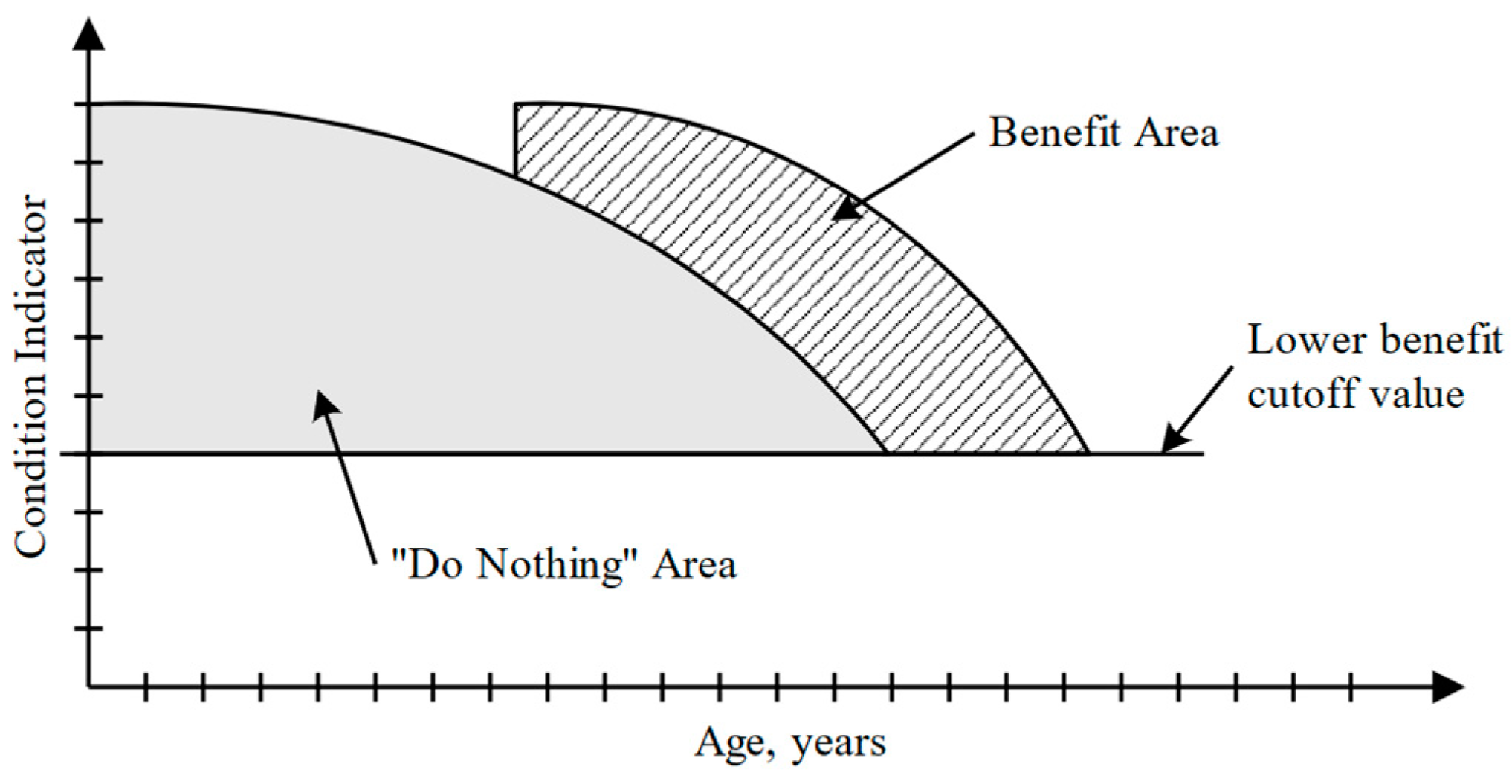
Pavement conditions can be defined in accordance with commonly accepted measures, such as PCI, IRI, PSI, or any custom-defined performance measure. The benefit of a pavement preventive maintenance treatment is calculated as the difference in the area beneath the performance curve due to the treatment application and that of the “do nothing” alternative (see Figure 1).

MBCR is expressed as a ratio of costs and benefits. The costs are in terms of unit costs. The benefit associated with the application of a maintenance treatment is based on the improvement in performance compared with that for the “do-nothing” alternative.

$$\mathrm{M}\mathrm{B}\mathrm{C}\mathrm{R}=\mathrm{B}\mathrm{e}\mathrm{n}\mathrm{e}\mathrm{f}\mathrm{i}\mathrm{t}/\mathrm{C}\mathrm{o}\mathrm{s}\mathrm{t}$$

(26)

3.2. Social Benefit Indicators

The social benefits brought by the maintenance plan mainly consider the extension of road surface service life and savings in user costs after the implementation of maintenance measures.

① Extension of road service life

The pavement’s life without preventive maintenance is ${\mathrm{T}}_{\mathrm{n}}$. The service life of the road surface after implementing some preventive maintenance when the road age is j is ${\mathrm{T}}_{\mathrm{a}}^{\mathrm{j}}$, then the calculation of the extension of pavement service life $∆{\mathrm{T}}^{\mathrm{j}}$ is as follows [8]:

$$∆{\mathrm{T}}^{\mathrm{j}}={\mathrm{T}}_{\mathrm{a}}^{\mathrm{j}}-{\mathrm{T}}_{\mathrm{n}}$$

(27)

② Road user cost savings

The cost savings in fuel consumption after pavement maintenance can be expressed as [22]

$$∆\mathrm{F}\mathrm{C}\mathrm{C}=\mathrm{Q}·{(\mathrm{F}\mathrm{C}}_0-{\mathrm{F}\mathrm{C}}_1)/100·{\mathrm{P}}_{\mathrm{F}}·\mathrm{l}$$

(28)

where

${\mathrm{F}\mathrm{C}}_0$—the fuel consumption of a single vehicle before maintenance.

${\mathrm{F}\mathrm{C}}_1$—the fuel consumption of a single vehicle after maintenance.

The cost savings in tire wear after pavement maintenance can be calculated using the following formula [22].

$$∆\mathrm{W}\mathrm{C}=\mathrm{Q}·\left({\mathrm{W}}_0-{\mathrm{W}}_1\right)/1000·{\mathrm{P}}_{\mathrm{T}}·\mathrm{l}$$

(29)

where

${\mathrm{W}}_0$—the tire wear of a single vehicle before maintenance.

${\mathrm{W}}_1$—the tire wear of a single vehicle after maintenance.

The cost savings in repair materials after pavement maintenance can be calculated using the following formula [22].

$$∆\mathrm{R}\mathrm{C}=\mathrm{Q}·\left({\mathrm{R}}_0-{\mathrm{R}}_1\right)/1000·{\mathrm{P}}_{\mathrm{R}}·\mathrm{l}$$

(30)

where

${\mathrm{R}}_0$—The ratio of maintenance cost per kilometer for 1000 vehicles before maintenance to the price of a new car

${\mathrm{R}}_1$—The ratio of maintenance cost per kilometer for 1000 vehicles after maintenance to the price of a new car

The savings in user travel time cost after implementing pavement maintenance ΔT can be expressed by the following equation [22]:

$$∆\mathrm{T}\mathrm{T}\mathrm{C}=\mathrm{Q}·{(\mathrm{T}}_0-{\mathrm{T}}_1)·\mathsf{\theta }$$

(31)

where

T0—the travel time of a single vehicle before maintenance.

T1—the travel time of a single vehicle after maintenance.

The savings in accident cost after implementing pavement maintenance ΔAC can be expressed by the following Equation (32) [22]:

$$∆\mathrm{A}\mathrm{C}={(\mathrm{A}\mathrm{T}}_0-{\mathrm{A}\mathrm{T}}_1)·{\mathrm{P}}_{\mathrm{A}}$$

(32)

where

${\mathrm{A}\mathrm{T}}_0$—The number of accidents before maintenance.

${\mathrm{A}\mathrm{T}}_1$—The number of accidents after maintenance.

3.3. Environmental Benefit Indicators

The cost savings in emission costs after pavement maintenance can be expressed as

$$∆{\mathrm{E}\mathrm{E}\mathrm{C}}_{\mathrm{j}}=({\mathrm{E}\mathrm{E}}_{\mathrm{j}0}-{\mathrm{E}\mathrm{E}}_{\mathrm{j}1})\times {\mathrm{P}}_{\mathrm{E},\mathrm{j}}$$

(33)

where

${\mathrm{E}\mathrm{E}}_{\mathrm{j}0}$—emissions of environmental emissions j before maintenance

${\mathrm{E}\mathrm{E}}_{\mathrm{j}1}$—emissions of environmental emissions j after maintenance

The cost savings in energy consumption cost after pavement maintenance can be expressed as

$${∆\mathrm{N}\mathrm{C}}_{\mathrm{o}\mathrm{p}\mathrm{e}\mathrm{r}}=\mathrm{Q}\times {(\mathrm{F}\mathrm{C}}_0-{\mathrm{F}\mathrm{C}}_1)/100\times \mathrm{R}\times \mathrm{l}\times {\mathrm{P}}_{\mathrm{N}}$$

(34)

where

${\mathrm{F}\mathrm{C}}_0$—the fuel consumption of a single vehicle before maintenance.

${\mathrm{F}\mathrm{C}}_1$—the fuel consumption of a single vehicle after maintenance.

3.4. Maintenance Benefit Evaluation System Based on AHP Model

The various evaluation indicators for evaluating maintenance benefits have already been proposed in the previous text, which makes it crucial to use comprehensive analysis and evaluation of each indicator. Given the diversity of maintenance benefit evaluation objectives, traditional weighting methods find it difficult to coordinate the weights of various indicators. The analytic hierarchy process (AHP) can effectively solve decision-making problems with complex structures and multiple decision-making criteria. It is a systematic decision-making method that transforms problems from qualitative analysis to quantitative analysis and can effectively calculate the weight of the comprehensive evaluation model for maintenance benefits.

According to the basic usage process of the AHP method, it can be divided into three steps: constructing a hierarchical structure model; construct a judgment matrix; model weight calculation.

① Hierarchy model.

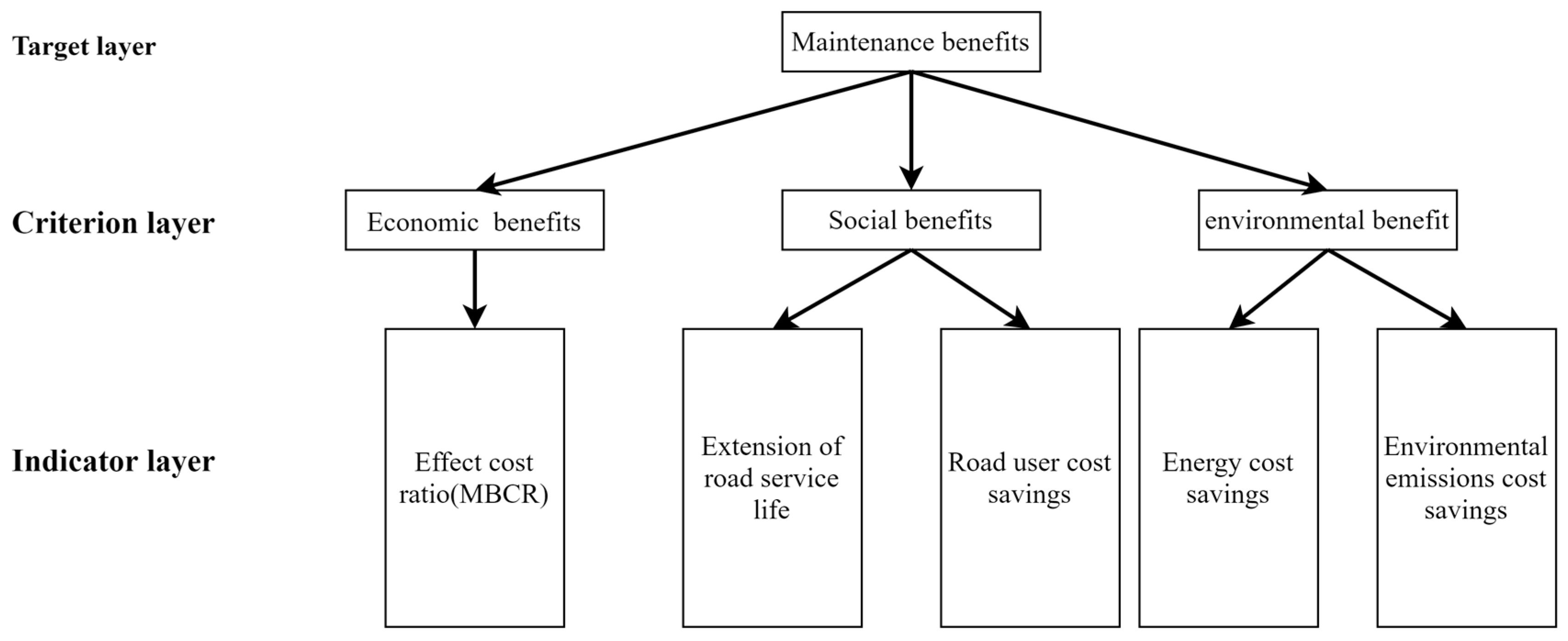
AHP reflects the hierarchical relationship of the model through the established hierarchical model. Among them, the highest level of the model is the target level, that is, maintenance benefits, the middle layer is the criterion layer composed of maintenance economic benefits; social benefits, and environmental benefits; and the lowest level is the index layer composed of various benefit indicators, as shown in Figure 2.

② Constructing a judgment matrix

The construction of the judgment matrix is the core part of the analytic hierarchy method, and the decision-makers are based on the AHP maintenance benefit evaluation hierarchy model, comprehensive advice, research, and calculation results of owners and experts, and compare the elements of the next layer one by one based on the goals of the previous layer, analyze the relative importance of the factors of each layer, and determine the importance of the next layer of elements to the goals of the previous layer. The construction method of each layer judgment matrix often adopts the 1–9 scale method shown in

Table 9. Definition of Judgment Index Scale.

Scale	Definition
1	Factor i is equally important as factor j
3	Factor i is slightly more important than factor j
5	Factor i is stronger and more important than factor j
7	Factor i is more important than factor j
9	Factor i and factor j are absolutely important
2, 4, 6, 8	Judgment value between adjacent degrees
count backwards	The comparison between factor j and factor i shows a reciprocal relationship of 7 with the comparison between factor i and factor j

.

a. Criterion layer judgment matrix

The criterion layer mainly includes three aspects of benefits: economic benefits, social benefits, and environmental benefits. The judgment matrix of the criterion layer is shown in

Table 10. Judgment Matrix of Criterion Layer.

Maintenance Benefits	Economic Benefits	Social Benefits	Environmental Benefit
Economic benefits	1	2	2
Social benefits	½	1	1
environmental benefit	½	1	1

[23]:

b. Indicator layer judgment matrix

In the construction of the indicator layer judgment matrix, the economic benefit indicator adopts the performance improvement value; the social benefit indicators adopt service life extension and road user cost savings; and the environmental benefit indicators adopt the cost savings of energy consumption and environmental emissions [36].

For road user cost savings, it is very necessary to save users’ time while driving on the road. At the same time, on the basis of saving time, it is necessary to ensure the safety of drivers and passengers before considering the operating cost of the vehicle [8]. Therefore, the judgment matrix of the social benefit indicator layer is constructed as shown in

Table 11. Judgment Matrix of Social Benefits.

Social Benefit Indicators	Extension of Road Service Life	Cost Savings in Vehicle Travel Time	Vehicle Fuel Consumption Cost Savings	Vehicle Accident Cost Savings
Extension of road service life	1	1	4	2
Cost savings in vehicle travel time	1	1	4	2
Vehicle operating cost savings	1/4	¼	1	1/3
Vehicle accident cost savings	1/2	½	3	1

. The judgment matrix for constructing the indicator layer of environmental benefit indicators is shown in

Table 12. Judgment Matrix of Environmental Benefits.

Environmental Benefit Indicators	Emission Savings	Energy Consumption Savings
Emission savings	1	2
Energy consumption savings	½	1

[36].

c. Vehicle operating cost and environmental emission judgment matrix

Vehicle operating costs mainly include fuel consumption costs, tire wear costs, and warranty material consumption costs. Considering that the cost of warranty material consumption involves repairing the vehicle’s condition, priority should be given to avoiding this part of the cost, while fuel consumption and tire wear are inevitable. In real life, compared to fuel consumption costs, tire wear costs are relatively low [8]. The obtained judgment matrix obtained is shown in

Table 13. Vehicle operating cost savings judgment matrix.

Vehicle Operating Cost Savings	Vehicle Fuel Consumption Cost Savings	Tire Wear Cost Savings	Savings in Warranty Material Consumption Costs
Vehicle fuel consumption cost savings	1	3	1/2
Tire wear cost savings	1/3	1	1/5
Savings in warranty material consumption costs	2	5	1

.

Based on expert ratings, the judgment matrix for the four secondary indicators in environmental emission indicators is obtained as follows (

Table 14. Environmental emission indicator judgment matrix.

Environmental Emissions	CO2	HC	NOx	CO
CO2	1	3	5	4
HC	1/3	1	3	2
NOx	1/5	1/3	1	1/3
CO	1/4	1/2	3	1

) [9]:

③ Model weight calculation results

The eigenvectors calculated based on the above judgment matrix are the corresponding weights of the model. The weight coefficients of each layer in the comprehensive benefit calculation model are shown in

Table 15. Model weight coefficient.

Hierarchical Structure	Criterion Layer	Indicator Layer		Weighted Results
	${\mathrm{w}}_{\mathrm{E}\mathrm{c}\mathrm{o}\mathrm{n}\mathrm{o}\mathrm{m}\mathrm{i}\mathrm{c}}^{\mathrm{C}\mathrm{r}\mathrm{i}\mathrm{t}\mathrm{e}\mathrm{r}\mathrm{i}\mathrm{o}\mathrm{n}}=$ 0.500	${\mathrm{w}}_{\mathrm{A}}^{\mathrm{I}\mathrm{n}\mathrm{d}\mathrm{i}\mathrm{c}\mathrm{a}\mathrm{t}\mathrm{o}}=1$		0.500
weight coefficient	${\mathrm{w}}_{\mathrm{S}\mathrm{o}\mathrm{c}\mathrm{i}\mathrm{a}\mathrm{l}}^{\mathrm{C}\mathrm{r}\mathrm{i}\mathrm{t}\mathrm{e}\mathrm{r}\mathrm{i}\mathrm{o}\mathrm{n}}=$ 0.250	${\mathrm{w}}_{{\mathrm{B}}_1}^{\mathrm{I}\mathrm{n}\mathrm{d}\mathrm{i}\mathrm{c}\mathrm{a}\mathrm{t}\mathrm{o}}=0.3593$		0.090
		${\mathrm{w}}_{{\mathrm{B}}_2}^{\mathrm{I}\mathrm{n}\mathrm{d}\mathrm{i}\mathrm{c}\mathrm{a}\mathrm{t}\mathrm{o}}=0.3593$		0.090
		${\mathrm{w}}_{\mathrm{B}3}^{\mathrm{I}\mathrm{n}\mathrm{d}\mathrm{i}\mathrm{c}\mathrm{a}\mathrm{t}\mathrm{o}}=0.0815$	${\mathrm{w}}_{3-1}^{{\mathrm{B}}_3}=0.3090$	0.006
			${\mathrm{w}}_{3-2}^{{\mathrm{B}}_5}=0.1095$	0.002
			${\mathrm{w}}_{3-3}^{{\mathrm{B}}_3}=0.5816$	0.012
		${\mathrm{w}}_{{\mathrm{B}}_4}^{\mathrm{I}\mathrm{n}\mathrm{d}\mathrm{i}\mathrm{c}\mathrm{a}\mathrm{t}\mathrm{o}}=0.1999$		0.050
	${\mathrm{w}}_{\mathrm{E}\mathrm{n}\mathrm{v}\mathrm{i}\mathrm{r}\mathrm{o}\mathrm{n}\mathrm{m}\mathrm{e}\mathrm{n}\mathrm{t}}^{\mathrm{C}\mathrm{r}\mathrm{i}\mathrm{t}\mathrm{e}\mathrm{r}\mathrm{i}\mathrm{o}\mathrm{n}}=$ 0.250	${\mathrm{w}}_{{\mathrm{C}}_1}^{\mathrm{I}\mathrm{n}\mathrm{d}\mathrm{i}\mathrm{c}\mathrm{a}\mathrm{t}\mathrm{o}}=0.67$	${\mathrm{w}}_{1-1}^{{\mathrm{C}}_1}=0.5409$	0.091
			${\mathrm{w}}_{1-2}^{{\mathrm{C}}_1}=0.2298$	0.038
			${\mathrm{w}}_{1-3}^{{\mathrm{C}}_1}=0.0758$	0.013
			${\mathrm{w}}_{1-4}^{{\mathrm{C}}_1}=0.1535$	0.026
		${\mathrm{w}}_{{\mathrm{C}}_2}^{\mathrm{I}\mathrm{n}\mathrm{d}\mathrm{i}\mathrm{c}\mathrm{a}\mathrm{t}\mathrm{o}}=0.33$		0.082

.

According to the model weight coefficient obtained in Table 9, the specific calculation formula of the comprehensive maintenance benefit model is obtained, as shown in Formula (35).

$$\begin{gathered} \mathrm{A}=0.5\times \mathrm{M}\mathrm{B}\mathrm{C}\mathrm{R}+0.09\times ∆{\mathrm{T}}^{\mathrm{j}}+(0.09\times ∆\mathrm{T}\mathrm{T}\mathrm{C}+0.006\times ∆\mathrm{F}\mathrm{C}\mathrm{C}+0.002\times ∆\mathrm{W}\mathrm{C}+0.012\times ∆\mathrm{R}\mathrm{C}+0.05\times ∆\mathrm{A}\mathrm{C}+ \\ 0.091\times ∆{\mathrm{E}\mathrm{E}\mathrm{C}}_{\mathrm{C}\mathrm{O}2}+0.038\times ∆{\mathrm{E}\mathrm{E}\mathrm{C}}_{\mathrm{H}\mathrm{C}}+0.013\times ∆{\mathrm{E}\mathrm{E}\mathrm{C}}_{\mathrm{N}\mathrm{O}\mathrm{x}}+0.026\times ∆{\mathrm{E}\mathrm{E}\mathrm{C}}_{\mathrm{C}\mathrm{O}}+0.082\times {∆\mathrm{N}\mathrm{C}}_{\mathrm{o}\mathrm{p}\mathrm{e}\mathrm{r}}) \end{gathered}$$

(35)

Define the bracket part of the comprehensive benefit calculation Formula (35) as the cost difference (CD), that is, the difference between the cost of pavement use before maintenance and the cost of pavement use after maintenance. Then Formula (35) can be expressed as:

$$\mathrm{A}=0.5\times \mathrm{M}\mathrm{B}\mathrm{C}\mathrm{R}+0.09\times ∆{\mathrm{T}}^{\mathrm{j}}+\mathrm{C}\mathrm{D}$$

(36)

For Equation (36), different evaluation indicators have different units, and in order to make the comprehensive benefits of the final calculation comparable, it is first necessary to standardize different indicators. The purpose of maximizing is to use the maximum value as a reference standard, dividing all data by the maximum value. The calculation formula is X/Max, which means taking the maximum value as the unit and removing all data from the maximum value.

$${\mathrm{A}}^{\prime }=0.5\times {\mathrm{M}\mathrm{B}\mathrm{C}\mathrm{R}}^{\prime }+0.09\times ∆{\mathrm{T}}^{\mathrm{j}}{}^{\prime }+{\mathrm{C}\mathrm{D}}^{\prime }$$

(37)

where

${\mathrm{M}\mathrm{B}\mathrm{C}\mathrm{R}}^{\prime }$, $∆{\mathrm{T}}^{\mathrm{j}}{}^{\prime }$, CD′—Original data dimensionalized value.

4. Determination of Optimal Timing

This study establishes the cost framework in the whole life cycle, gives the benefit model before and after maintenance, and takes the time when the benefit–cost ratio before and after maintenance in the whole life cycle is the best as the best time for maintenance.

The construction process for the preventive maintenance timing decision model is as follows:

4.1. Assumptions

In order to ensure the rationality and effectiveness of the modeling, the following assumptions are made during the model-building process:

① The induced increase in traffic volume due to the change in road performance after maintenance is not considered;

② Before and after the implementation of the maintenance project, the road section toll will not change;

③ There is no overhaul project caused by force majeure during the whole service life of the maintenance road section.

4.2. Life Cycle Cost Calculation

$${\mathrm{P}\mathrm{V}\mathrm{C}}_{{\mathrm{x}}_{\mathrm{i}},\mathrm{n}}={\mathrm{I}\mathrm{C}\mathrm{C}}_{{\mathrm{x}}_{\mathrm{i}}}+{\sum }_{\mathrm{t}=1}^{\mathrm{n}}{\mathrm{p}\mathrm{w}\mathrm{f}}_{\mathrm{i},\mathrm{t}}\left({\mathrm{M}\mathrm{C}}_{{\mathrm{x}}_{\mathrm{i}},\mathrm{t}}+{\mathrm{P}\mathrm{M}\mathrm{C}}_{{\mathrm{x}}_{\mathrm{i}},\mathrm{t}}+{\mathrm{U}\mathrm{C}}_{{\mathrm{x}}_{\mathrm{i}},\mathrm{t}}+{\mathrm{E}\mathrm{C}}_{{\mathrm{x}}_{\mathrm{i}},\mathrm{t}}\right)-{\mathrm{p}\mathrm{w}\mathrm{f}}_{\mathrm{i},\mathrm{n}}·{\mathrm{S}\mathrm{V}}_{\mathrm{i},\mathrm{n}}$$

(38)

where

${\mathrm{P}\mathrm{V}\mathrm{C}}_{{\mathrm{x}}_{\mathrm{i}},\mathrm{n}}$ (Present value of future costs)—the present value of the total cost of plan x_i in n years within the analysis period, and the life of the plan with the shortest life is taken as the analysis period.

${\mathrm{I}\mathrm{C}\mathrm{C}}_{{\mathrm{x}}_{\mathrm{i}}}$ (Initial construction costs)—the initial construction cost of plan ${\mathrm{x}}_{\mathrm{i}}$

${\mathrm{M}\mathrm{C}}_{{\mathrm{x}}_{\mathrm{i}},\mathrm{t}}$ (Maintenance costs)—the routine maintenance cost of plan ${\mathrm{x}}_{\mathrm{i}}$ in year t

${\mathrm{P}\mathrm{M}\mathrm{C}}_{{\mathrm{x}}_{\mathrm{i}},\mathrm{t}}$ (preventive maintenance cost)—the preventive maintenance cost of plan ${\mathrm{x}}_{\mathrm{i}}$ in year t

${\mathrm{U}\mathrm{C}}_{{\mathrm{x}}_{\mathrm{i}},\mathrm{t}}$ (User costs)—the user costs of plan ${\mathrm{x}}_{\mathrm{i}}$ in year t

${\mathrm{E}\mathrm{C}}_{{\mathrm{x}}_{\mathrm{i}},\mathrm{t}}$ (Environment costs)—the environmental cost of plan ${\mathrm{x}}_{\mathrm{i}}$ in year t

${\mathrm{p}\mathrm{w}\mathrm{f}}_{\mathrm{i},\mathrm{n}}$ (present worth factor)—the present value factor of discount rate i in year t. The discount rate is generally 8% [7].

$${\mathrm{p}\mathrm{w}\mathrm{f}}_{\mathrm{i},\mathrm{n}}=1/{(1+\mathrm{i})}^{\mathrm{t}}$$

(39)

4.3. Life Cycle Benefit Calculation

$${\mathrm{B}\mathrm{C}}_{{\mathrm{x}}_{\mathrm{i}},\mathrm{n}}=({\sum }_{\mathrm{t}=1}^{\mathrm{n}}{\mathrm{p}\mathrm{w}\mathrm{f}}_{\mathrm{i},\mathrm{t}}·{\mathrm{C}\mathrm{D}}_{{\mathrm{x}}_{\mathrm{i}},\mathrm{t}}){}^{\prime }+0.5\times \mathrm{M}\mathrm{B}\mathrm{C}\mathrm{R}{}^{\prime }+0.09\times ∆{\mathrm{T}}^{\mathrm{j}}{}^{\prime }$$

(40)

where

${\mathrm{B}\mathrm{C}}_{{\mathrm{x}}_{\mathrm{i}},\mathrm{n}}$—Comprehensive benefits after maintenance in the whole life cycle;

${\mathrm{C}\mathrm{D}}_{{\mathrm{x}}_{\mathrm{i}},\mathrm{t}}$—The difference between the cost of pavement after maintenance and the cost of unmaintained pavement in the i year of plan ${\mathrm{x}}_{\mathrm{i}}$

4.4. Calculation of Optimal Maintenance Timing

The cost–benefit ratio method is used to determine optimal maintenance timing. When the cost–benefit ratio is at its maximum, the corresponding road age is the optimal time for implementing preventive maintenance. The calculation method is shown in the Formula (41).

$${\mathrm{T}}_{\mathrm{t}}=\mathrm{Maximize} (\frac{{\mathrm{B}\mathrm{C}}_{{\mathrm{x}}_{\mathrm{i}},\mathrm{n}}}{{\mathrm{P}\mathrm{V}\mathrm{C}}_{{\mathrm{x}}_{\mathrm{i}},\mathrm{n}}})$$

(41)

where

T_t—The best timing for implementing preventive maintenance on road sections;

5. Case Study Implementation of the Decision-Support Framework

5.1. Brief of Case Study

The highway is constructed with asphalt concrete pavement, and the entire line adopts a fully enclosed, two-way, four-lane highway construction standard. The designed driving speed is 100 km/h. In order to maintain a good level of road conditions, it has been decided to carry out preventive maintenance on its slurry seal layer, starting in 2014 as the analysis cycle and selecting the best maintenance time through analysis and evaluation.

5.2. Data Collection

• Work Zone Characteristics

Work zone capacity was observed from the highway capacity manual (HCM) 2000. The construction duration is 23 days, and the enclosure will not be removed during the construction period. During the construction period, a one-way, one-lane road will be closed with a speed limit of 80 km/h.

• Traffic Characteristics

The historical traffic volume data was obtained from traffic counting stations. Passenger vehicles were classified into passenger cars and passenger buses, accounting for 75% and 25%, respectively. Truck vehicles were classified into light-duty trucks and heavy-duty trucks, accounting for 55% and 45%, respectively.

5.3. Calculation of Effect and Life Extension

According to the predicted road conditions and traffic volume, and based on local experience, a 1 cm slurry seal is adopted as the maintenance plan, and the maintenance timing is when the pavement life is 4, 5, 6, or 7 years (calculated from 2014). Corresponding plans 1, 2, 3, and 4.

5.3.1. Select Pavement Condition Indicators

Due to limited data collection, the effectiveness of the slurry seal layer is measured by the pavement condition index (PCI). According to the “Technical Specification for Highway Asphalt Pavement Maintenance” [23], the minimum acceptable levels of various indicators of asphalt pavement maintenance quality standards are shown in

Table 16. Minimum Acceptable Levels of pavement Condition Indicators.

Indicators	The Lowest Acceptable Level
PCI	≥70
IRI	≤6

.

5.3.2. Decay Curve without Preventive Maintenance Measures

Based on the surveyed pavement condition data, the decay curve equations of PCI and IRI can be regressed when no maintenance measures are taken. As shown in

Table 17. Decay curve without preventive maintenance measures.

Indicators	Decay Curve
PCI	$\mathrm{y}=100\times {\mathrm{e}}^{-0.047\mathrm{x}}$
IRI	$\mathrm{y}=1.73\times {\mathrm{e}}^{0.06\mathrm{x}}$

.

5.3.3. Decay Curve after Preventive Maintenance Measures

Based on the data collected when using slurry seal as a preventive maintenance measure under similar road conditions, the empirical regression method is used to predict the decay of PCI and IRI after using slurry seal as a maintenance measure (x in the decay curve is calculated from the preventive maintenance measure). As shown in

Table 18. Decay curve after preventive maintenance measures.

	Decay Curve	PCI	IRI
Road Age
4		$\mathrm{y}=100 \times {\mathrm{e}}^{-0.0583\mathrm{x}}$	$\mathrm{y}=1.71 \times {\mathrm{e}}^{0.063\mathrm{x}}$
5		$\mathrm{y}=100{ \times \mathrm{e}}^{-0.0456\mathrm{x}}$	$\mathrm{y}=1.75{ \times \mathrm{e}}^{0.058\mathrm{x}}$
6		$\mathrm{y}=100{ \times \mathrm{e}}^{-0.0483\mathrm{x}}$	$\mathrm{y}=1.81{ \times \mathrm{e}}^{0.058\mathrm{x}}$
7		$\mathrm{y}=100{ \times \mathrm{e}}^{-0.0556\mathrm{x}}$	$\mathrm{y}=1.83{ \times \mathrm{e}}^{0.063\mathrm{x}}$

.

5.3.4. Calculation of Time to Reach the Lowest Acceptable Level

From the predicted results in the table, it can be seen that the time when IRI reaches the lowest acceptable level is later than PCI, so as long as the time when PCI reaches the lowest acceptable level is calculated, it is the time when this plan reaches the lowest acceptable level.

The years for each plan to reach the lowest acceptable level of preventive maintenance and the calculation of their respective life extensions are shown in

Table 19. The road age for PCI to reach the lowest acceptable level for each plan.

Decay Curve	X Value at the Lowest Acceptable Level	Road Age at the Lowest Acceptable Level	Life Extension
$\mathrm{y}=100 \times {\mathrm{e}}^{-0.047\mathrm{x}}$	7.5	7.5	0
$\mathrm{y}=100{ \times \mathrm{e}}^{-0.0583\mathrm{x}}$	6.1	10.1	2.6
$\mathrm{y}=100{ \times \mathrm{e}}^{-0.0456\mathrm{x}}$	7.8	12.8	5.3
$\mathrm{y}=100{ \times \mathrm{e}}^{-0.0483\mathrm{x}}$	7.4	13.4	5.9
$\mathrm{y}=100{ \times \mathrm{e}}^{-0.0556\mathrm{x}}$	6.4	13.4	5.9

:

According to Table 19, the analysis period is the road service life of the plan that first reaches the lowest acceptable level of preventive maintenance measures, so the analysis period of LCCA is 10 years.

5.3.5. Calculation of the Effectiveness of Each Plan

Calculate the area A1 between PCI and the lowest acceptable level when no maintenance measures are taken, as follows:

$${\mathrm{A}\mathrm{R}\mathrm{E}\mathrm{A}}_0={\int }_0^{7.5}({100\times \mathrm{e}}^{-0.0473\mathrm{x}}-70)\mathrm{d}\mathrm{x}=106.4$$

The absolute values of the area increase enclosed by PCI and the lowest acceptable level after maintenance are: Plan 1: 64.34, Plan 2: 85.97, Plan 3: 79.7, and Plan 4: 65.82, indicating that the improvement effect of road performance is 60.47%, 80.80%, 74.91%, and 61.86%.

5.4. Cost Calculation for Different Plans

5.4.1. Agency Cost Calculation

(1) Routine maintenance costs

Based on the daily maintenance costs of 1.1, 1.27, and 1.41 yuan/(m² · year), traffic volume, and PCI data invested by the local maintenance department on this road from 2017 to 2019, the coefficients of Formula (1) were calibrated using the least squares method, and a = 0.72 and b = $3.44\times {10}^{-6}$ were obtained, indicating that the daily maintenance cost model is:

$${\mathrm{M}\mathrm{C}}_{\mathrm{i}}=0.72+3.44\times {10}^{-6}·(100-{\mathrm{P}\mathrm{C}\mathrm{I}}_{\mathrm{i}}){\mathrm{A}\mathrm{A}\mathrm{D}\mathrm{T}}_{\mathrm{i}}$$

(2) Preventive maintenance costs

Since we are conducting a life cycle cost analysis on the maintenance project on this road, the initial construction cost is the same. We can assume that the initial construction cost is zero, but the cost of preventive maintenance measures varies. Based on local experience and quota calculations, the cost of a domestic slurry seal layer with a thickness of 1 cm is 27,531 yuan/km.

(3) salvage value

The salvage value is calculated according to Formula (2), and the specific calculation results are shown in

Table 20. Calculation results of salvage value of each plan.

Maintenance Plan	${\mathbf{L}}_{\mathbf{A}}/\mathbf{y}\mathbf{e}\mathbf{a}\mathbf{r}$	${\mathbf{L}}_{\mathbf{E}/\mathbf{y}\mathbf{e}\mathbf{a}\mathbf{r}}$	SV/(10,000 yuan/km)
plan 1	6	6.1	0.4513
plan 2	5	7.8	9.8830
plan 3	4	7.4	12.6494
plan 4	3	6.4	14.6258

.

5.4.2. User Costs

(1) Normal operation user costs

Based on the traffic volume, PCI, and IRI data of Plan 1, the user costs for Plan 1 are calculated using Equations (2)–(12). The other methods are the same, and the normal operation user costs during the analysis period of plan 1 are shown in

Table 21. Calculation table of normal operation user cost of plan 1 (10,000 yuan/km).

Year	$\mathbf{F}\mathbf{C}\mathbf{C}$	$\mathbf{W}\mathbf{C}$	$\mathbf{R}\mathbf{C}$	$\mathbf{T}\mathbf{T}\mathbf{C}$	$\mathbf{A}\mathbf{C}$
1	294.1211	17.4257	0.00154	33.3285	6.1727
2	324.8908	19.2620	0.00154	38.2515	6.6986
3	358.9778	21.2982	0.00155	43.8971	7.2670
4	396.7672	23.5581	0.00156	50.36925	7.8796
5	430.3811	25.4968	0.00153	49.28365	9.0551
6	475.5033	28.1896	0.00154	57.12204	9.8205
7	525.4778	31.1757	0.00155	66.18907	10.645
8	580.8947	34.4909	0.00156	76.67867	11.534
9	642.369	38.1729	0.00156	88.80832	12.491
10	710.544	42.2615	0.00157	102.8211	13.518

.

(2) Work zone Additional User costs

According to the traffic volume of plan 1, the additional user costs for the work zone are calculated using Equations (13)–(18). The other methods are the same, and the additional fuel consumption cost of plan 1 in the analysis period is 157,600 yuan/km; the additional time delay cost is 50,300 yuan/km.

5.4.3. Quantitative Analysis of Life Cycle Energy Consumption and Environmental Emissions

(1) Normal operation Energy Consumption and Environmental Emissions

According to the normal operation fuel consumption of plan 1, Equations (19)–(21) and Table 8 are used to calculate energy consumption and environmental emissions for Plan 1. The other methods are the same, and the normal operation energy consumption and environmental emission costs of plan 1 during the analysis period are shown in

Table 22. Calculation of the normal operation Energy Consumption and Environmental Emission Costs of plan 1 (10,000 yuan/km).

Year	${\mathbf{E}\mathbf{E}\mathbf{C}}_{{\mathbf{C}\mathbf{O}}_2}$	${\mathbf{E}\mathbf{E}\mathbf{C}}_{\mathbf{H}\mathbf{C}}$	${\mathbf{E}\mathbf{E}\mathbf{C}}_{\mathbf{N}\mathbf{O}\mathbf{x}}$	${\mathbf{E}\mathbf{E}\mathbf{C}}_{\mathbf{C}\mathbf{O}}$	${\mathbf{N}\mathbf{C}}_{\mathbf{o}\mathbf{p}\mathbf{e}\mathbf{r}}$
1	3.131607	0.154784	6.368233	0.011757	427.644
2	3.459422	0.171009	7.035792	0.012979	472.410
3	3.82261	0.188989	7.775523	0.014332	522.008
4	4.225284	0.208928	8.595856	0.01583	576.998
5	4.582375	0.226486	9.318247	0.017205	625.756
6	5.063108	0.250281	10.29725	0.018997	691.406
7	5.595587	0.276643	11.38185	0.02098	764.122
8	6.186111	0.305886	12.58495	0.023176	844.765
9	6.841251	0.338336	13.92001	0.025611	934.232
10	7.567882	0.374336	15.40114	0.028307	1033.461

.

(2) Environmental emissions and energy consumption costs of maintenance activities

Referring to the “Highway Engineering Budget Quota” (JTG/T B06-02-2007) and “Highway Engineering Machinery Shift Cost Quota” (JTG/TB06-03-2007), the energy consumption during the production, transportation, and construction stages of slurry seal raw materials, as well as the fuel consumption of various machinery, can be calculated by combining equation (16), the unit price of environmental emissions, and the energy consumption unit price. The calculation results are shown in

Table 23. Environmental emissions and energy consumption costs of maintenance activities (10,000 yuan/km).

CO2 Emission Costs	HC Emission Costs	NOx Emission Costs	CO Emission Costs	Energy Consumption Costs
0.001884	8.13375 × 10−5	0.003349	0.000011	0.26043

.

(3) Additional environmental emissions and energy consumption in the work zone

According to the additional fuel consumption in the construction area of plan 1, Equations (22)–(25) are used to calculate energy consumption and environmental emissions for plan 1. The other methods are the same, and the additional energy consumption and environmental emission costs for the work zone of plan 1 are shown in

Table 24. Additional Energy Consumption and Environmental Emission Costs in the work zone (10,000 yuan/km).

CO2 Emission Costs	HC Emission Costs	NOx Emission Costs	CO Emission Costs	Energy Consumption Costs
0.172170	0.009020	0.371019	0.000458	23.53

.

5.4.4. Present Cost

Based on the above calculation results, the expenses incurred by the four plans at different times are converted into present value (based on 2014) using a discount coefficient of 8%. List only the present value of the cost for plan 1, as shown in

Table 25. Calculation of Present Value of Plan 1 Costs (10,000 yuan/km).

Year	Normal Operation									Work Zone				Maintenance Activities		SV
	$\mathbf{P}\mathbf{M}\mathbf{C}$	$\mathbf{M}\mathbf{C}$	$\mathbf{F}\mathbf{C}\mathbf{C}$	$\mathbf{W}\mathbf{C}$	$\mathbf{R}\mathbf{C}$	$\mathbf{T}\mathbf{T}\mathbf{C}$	$\mathbf{A}\mathbf{C}$	${\mathbf{N}\mathbf{C}}_{\mathbf{o}\mathbf{p}\mathbf{e}\mathbf{r}}$	${\mathbf{E}\mathbf{E}\mathbf{C}}_{\mathbf{o}\mathbf{p}\mathbf{e}\mathbf{r}}$	${\mathbf{F}\mathbf{C}\mathbf{C}}_{\mathbf{W}\mathbf{Z}}$	$\mathbf{D}\mathbf{T}\mathbf{C}$	${\mathbf{N}\mathbf{C}}_{\mathbf{W}\mathbf{Z}}$	${\mathbf{E}\mathbf{E}\mathbf{C}}_{\mathbf{W}\mathbf{Z}}$	Energy Consumption Costs	Emission Costs
1		1.111	272.3	16.13	0.00142	30.85	5.715	395.9	8.95
2		1.148	278.5	16.51	0.00132	32.79	5.742	405.0	9.15
3		1.189	284.9	16.90	0.00123	34.84	5.768	414.3	9.36
4		1.234	291.6	17.31	0.00114	37.02	5.791	424.1	9.58
5	18.7371	0.882	292.9	17.35	0.00104	33.54	6.162	425.8	9.62	10.725	3.4233	16.014	0.3761	0.1772	0.0036
6		0.972	299.6	17.76	0.00097	35.99	6.188	435.7	9.84
7		1.063	306.6	18.19	0.00090	38.62	6.211	445.8	10.07
8		1.155	313.8	18.63	0.00084	41.42	6.231	456.4	10.31
9		1.248	321.3	19.09	0.00078	44.42	6.248	467.3	10.56
10		1.342	329.1	19.57	0.00073	47.62	6.261	478.6	10.82							0.2090

.

5.5. Benefits

5.5.1. Effect Cost Ratio

Based on the effectiveness calculation results in 5.3.5, combined with the cost present value calculation results in Table 19, the effectiveness cost ratios of the four plans are calculated according to Equation (26). The calculation results are shown in

Table 26. Effectiveness cost ratios.

Plan	Effectiveness (%)	Cost (10,000 yuan/km)	Effectiveness Cost Ratio
1	60.47%	8114.228	0.007452
2	80.80%	8082.658	0.009997
3	74.91%	8109.177	0.009238
4	61.86%	10,668.19	0.005799

.

5.5.2. Social and Environmental Benefits

According to Formulas (28)–(34), calculate the social and environmental benefits of the four schemes at different times and convert them into present value (based on 2014) using a discount coefficient of 8%. List only the present value of the benefits of Plan 1, as shown in

Table 27. Calculation Table for Present Value of Benefits.

Year	$∆\mathbf{F}\mathbf{C}\mathbf{C}$	$∆\mathbf{W}\mathbf{C}$	$∆\mathbf{R}\mathbf{C}$	$∆\mathbf{T}\mathbf{T}\mathbf{C}$	$∆\mathbf{A}\mathbf{C}$	${∆\mathbf{E}\mathbf{E}\mathbf{C}}_{\begin{array}{c}\mathbf{oper} \\ {\mathbf{C}\mathbf{O}}_2\end{array}}$	$∆{\mathbf{E}\mathbf{E}\mathbf{C}}_{\begin{array}{c}\mathbf{o}\mathbf{p}\mathbf{e}\mathbf{r} \\ \mathbf{H}\mathbf{C}\end{array}}$	${∆\mathbf{E}\mathbf{E}\mathbf{C}}_{\begin{array}{c}\mathbf{o}\mathbf{p}\mathbf{e}\mathbf{r} \\ {\mathbf{N}\mathbf{O}}_{\mathbf{x}}\end{array}}$	${∆\mathbf{E}\mathbf{E}\mathbf{C}}_{\begin{array}{c}\mathbf{o}\mathbf{p}\mathbf{e}\mathbf{r} \\ \mathbf{C}\mathbf{O}\end{array}}$	${∆\mathbf{N}\mathbf{C}}_{\mathbf{o}\mathbf{p}\mathbf{e}\mathbf{r}}$
1	0	0	0	0	0	0	0	0	0	0
2	0	0	0	0	0	0	0	0	0	0
3	0	0	0	0	0	0	0	0	0	0
4	0	0	0	0	0	0	0	0	0	0
5	5.61	0.1052	2.03 × 10−5	5.784	0.351	0.0606	0.0030	0.1270	0.00019	8.28
6	6.00	0.1013	1.98 × 10−5	5.765	0.360	0.0648	0.0033	0.1359	0.00020	8.86
7	6.42	0.1003	1.921 × 10−5	5.720	0.368	0.0693	0.0035	0.1454	0.00022	9.47
8	6.88	0.1015	1.87 × 10−5	5.645	0.376	0.0742	0.0037	0.1556	0.00023	10.14
9	7.36	0.1042	1.82 × 10−5	5.538	0.382	0.0794	0.0040	0.1665	0.00025	10.85
10	7.85	0.1081	1.77 × 10−5	5.393	0.387	0.0847	0.0043	0.1777	0.00027	11.58

.

According to the established comprehensive evaluation model for maintenance benefits, Formula (41) is used to calculate the comprehensive benefits of the four plans: Plan 1: 0.47, Plan 2: 0.65, Plan 3: 0.62, and Plan 4: 0.44

5.6. Choosing the Best Maintenance Time

The calculation results of the cost-effectiveness ratio are shown in

Table 28. Benefit Cost Ratio.

Time for Taking Maintenance Measures	Comprehensive Benefits	Present Cost	Benefit Cost Ratio
4	0.47	8114.22	5.8 × 10−3
5	0.65	8082.65	8.0 × 10−3
6	0.62	8109.17	7.6 × 10−3
7	0.44	10,668.18	4.0 × 10−3

.

From Table 22, it can be seen that when the pavement service life is five years, the cost-effectiveness ratio of adopting a slurry seal as a preventive maintenance measure is the highest. At this time, it is the best maintenance opportunity to adopt a slurry seal as a preventive maintenance measure.

6. Conclusions

Based on the analysis of the current research status of preventive maintenance timing decision-making at home and abroad, this study starts from the aspects of LCCA and LCA, establishes a comprehensive decision-making method and model for maintenance timing from economic, social, and environmental aspects, and selects maintenance plans with high economic efficiency and small environmental impact throughout the entire life cycle for maintenance projects. It also improve the scientific nature and sustainable development level of road maintenance decision-making. Through case analysis, the following conclusions can be drawn:

(1) Integrated LCCA and LCA by the principle that energy consumption and air pollutants, e.g., CO₂, HC, NOx, and CO, were assigned monetary values for unit mass. Then the environmental damage cost computed by multiplying unit price with energy consumption and air pollutant mass, together with agency cost and user cost, was treated as inputs for the LCCA.

(2) In the process of building the cost model, consider the costs caused by the maintenance and construction processes to users and the environment, and provide an improved calculation method to estimate the fuel consumption and environmental emissions associated with speed changes through the work zone areas.

(3) A functional relationship between user cost-saving benefits, environmental cost-saving benefits, and pavement performance was constructed. Considering the economic, social, and environmental benefits of each maintenance plan, a comprehensive evaluation model for highway pavement maintenance benefits was constructed using the AHP.

(4) The framework of life-cycle maintenance costs and benefits of asphalt pavement is expounded, and a decision-making model for maintenance timing is established from the aspect of maintenance benefit–cost ratio. And using the model constructed to determine the timing of preventive maintenance of asphalt pavement, practical application research on a certain expressway was carried out.

In addition, this study also has the following shortcomings: Firstly, although this article has constructed relevant calculation models for user cost savings and environmental cost savings, it has not accounted for other indirect benefits of road maintenance. Secondly, when constructing the optimal timing method for pavement preventive maintenance in this article, the analysis period is relatively short, and only one preventive maintenance is considered during the analysis period. The corresponding calculation method is not constructed for the optimal timing of multiple preventive maintenance activities within a longer analysis period. Finally, although this article categorizes maintenance benefits and systematically proposes evaluation indicators for maintenance benefits, it is still limited. For future research, more research should be conducted on the establishment and calculation of maintenance efficiency indicators.

References

1. Tu, R.H. An in-depth exploration of the FHWA highway noise prediction model in the United States. Environ. Eng. 1995, 13, 41–45. [Google Scholar]
2. Harford, J.D. Harford. Congestion, Pollution, and Benefit-to-Cost Ratios of US Public Transit Systems. Transp. Res. Part D 2006, 11, 45–58. [Google Scholar] [CrossRef]
3. Peshkin, D.; Hoerner, T. The Optimal Time for Preventive Maintenance: Concepts and Practice. In Proceedings of the 6th International Conference on Managing Pavements: The Lessons, The Challenges, The Way Ahead, Brisbane, QLD, Australia, 19–24 October 2004. [Google Scholar]
4. FHWA. Life Cycle Cost Analysis Primer. Off. Asset Manag. 2002, 8, 608–618. [Google Scholar]
5. Ozbay, K.; Jawad, D.; Parker, N. Life-Cycle Cost Analysis: State of the Practice Versus State of the Art. Transp. Res. Rec. J. Transp. Res. Board 2004, 1864, 62–70. [Google Scholar] [CrossRef]
6. Mao, X.H. Research on Improvement of Decision Model for Highway Pavement Maintenance; Chang’an University: Xi’an, China, 2015. [Google Scholar]
7. Ren, Y. Research on the Timing of Preventive Maintenance of Asphalt Pavement Based on Life Cycle Cost; Chang’an University: Xi’an, China, 2006. [Google Scholar]
8. Yao, Y.Q. Decision Research on Preventive Maintenance Behavior of Asphalt Pavement Based on the Whole Life Cycle; East China Jiaotong University: Nanchang, China, 2023. [Google Scholar]
9. Cui, W.B. Research on Preventive Maintenance Timing Based on the Decay Law of Pavement Performance; Chang’an University: Xi’an, China, 2011. [Google Scholar]
10. O’Brien, L.G. NCHRP Synthesis of Highway Practice 153: Evolution and Benefits of Preventive Maintenance Strategies; Transportation Research Board, National Research Council: Washington, DC, USA, 1989. [Google Scholar]
11. Wang, X.F. Research on the Timing and Strategy of Preventive Maintenance of Asphalt Pavement Based on Full Life Cycle Analysis; Lanzhou Jiaotong University: Lanzhou, China, 2013. [Google Scholar]
12. Santero, N.J.; Masanet, E.; Horvath, A. Life-cycle assessment of pavements—Part I: Critical review. Resour. Conserv. Recycl. 2011, 55, 801–809. [Google Scholar] [CrossRef]
13. Hkkinen, T.; Mäkelä, K. Environmental Adaption of Concrete: Environmental Impact of Concrete and Asphalt Pavements; VTT Technical Research Centre of Finland: Espoo, Finland, 1996. [Google Scholar]
14. Piantanakulchai, M.; Inamura, H.; Takeyama, Y. A life cycle inventory analysis of carbon dioxide for a highway construction project using input-output scheme a case study of the Tohoku expressway construction works. Infrastruct. Plan. Rev. 1999, 16, 411–418. [Google Scholar] [CrossRef]
15. Pan, M.P. Research and Application of LCA Based Calculation Method for Highway Energy Consumption and Carbon Emissions; Huazhong University of Science and Technology: Wuhan, China, 2011. [Google Scholar]
16. Huang, Y. Environmental Impact Analysis of Pavement Maintenance Using Life-Cycle Assessment and Microsimulation. In Proceedings of the Transportation Research Board 88th Annual Meeting, Washington, DC, USA, 11–15 January 2009. [Google Scholar]
17. Zhang, Q. Research on Environmental Assessment Method for Asphalt Pavement Maintenance Based on Life Cycle Theory; Beijing University of Technology: Beijing, China, 2015. [Google Scholar]
18. Milachowski, C.; Stengel, T.; Gehlen, C. Life cycle assessment for road construction and use. In Proceedings of the 11th International Symposium on Concrete Roads, Seville, Spain, 13–15 October 2010. [Google Scholar]
19. Sun, L.J. Theory of Structural Behavior of Asphalt Pavement; People’s Communications Press: Beijing, China, 2005. [Google Scholar]
20. Luo, F.Y.; Sun, L.J. Research on the Design Method of Asphalt Pavement Structure Based on Performance. J. China Highw. Eng. 2001, 4, 35–38. [Google Scholar]
21. Yao, Z.K. Road Management System; People’s Transportation Press: Beijing, China, 1993; pp. 74–80. [Google Scholar]
22. Meng, S.Y.; Shao, Y.Q.; Cao, R. Multi-objective optimization of network level pavement maintenance decision-making considering user costs. In Proceedings of the 2022 World Transportation Congress (WTC2022), Wuhan, China, 13–16 June 2022; People’s Communications Press: Beijing, China, 2022; pp. 693–701. [Google Scholar]
23. Xie, S.J. Research on the Evaluation Method of Expressway Asphalt Pavement Maintenance Efficiency; Southeast University: Nanjing, China, 2016. [Google Scholar]
24. Ahn, K. Microscopic Fuel Consumption and Emission Models; Virginia Polytechnic Institute and State University: Blacksburg, VA, USA, 1998. [Google Scholar]
25. Hao, C. Benefit Analysis and Application Research of Urban Rail Transit Projects; Beijing Jiaotong University: Beijing, China, 2008. [Google Scholar]
26. Chen, J.; Wang, Y.X. Economic Analysis of Construction Projects; Tongji University Press: Shanghai, China, 2009. [Google Scholar]
27. Guan, X.F.; Zhang, H.C.; Du, X.B.; Zhang, X.Y.; Sun, M.T.; Bi, Y.F. Optimization for Asphalt Pavement Maintenance Plans at Network Level: Integrating Maintenance Funds, Pavement Performance, Road Users, and Environment. Appl. Sci. 2023, 13, 8842. [Google Scholar] [CrossRef]
28. Liu, X.M.; He, Y.L.; Ren, F.T. Measurement method for quality of life loss of road traffic accident victims. Ergonomics 1996, 2, 15–21. [Google Scholar]
29. Mallela, J.; Sadasivam, S. Work Zone Road User Costs: Concepts and Applications. 2011. Available online: https://rosap.ntl.bts.gov/view/dot/41649 (accessed on 1 January 2011).
30. Zhang, K.; Batterman, S.; Dion, F. Vehicle emissions in congestion: Comparison of work zone, rush hour and free-flow conditions. Atmos. Environ. 2011, 45, 1929–1939. [Google Scholar] [CrossRef]
31. Federal Highway Administration. Life-Cycle Cost Analysis in Pavement Design; U.S. Department of Transportation: Washington, DC, USA, 1998.
32. Meng, L. Evaluation of Energy Consumption and Emissions of Asphalt Pavements in Heilongjiang Province Based on LCA; Northeast Forestry University: Harbin, China, 2018. [Google Scholar]
33. Traffic and Highway Engineering Quota Station, Ministry of Transport. Highway Engineering Budget Quota; People’s Communications Press: Beijing, China, 2007.
34. JTG/T B06-03-2007; Cost Quota for Highway Engineering Machinery Shift. Quota Station for Transportation and Highway Engineering. People’s Communications Press: Beijing, China, 2008.
35. Shanghai Highway Management Office. Technical Specification for Highway Asphalt Pavement Maintenance; People’s Communications Press: Beijing, China, 2001. [Google Scholar]
36. Ma, L. Research on the Comprehensive Evaluation System of Expressway Maintenance Cost Benefit; Southeast University: Nanjing, China, 2019. [Google Scholar]
Figure 1. Illustration of the do-nothing and benefit areas [35].
Applsci 13 10629 g001
Figure 2. AHP Maintenance Benefit Evaluation Hierarchy Model.
Applsci 13 10629 g002