
FEM Investigation of a Multi-Neck Helmholtz Resonator


Abstract
:1. Introduction
2. Background
2.1. Langfeldt et al. [33] Theoretical Formulation
2.2. FEM Formulation and Setup
2.3. Lumped-Element Approximation (Single Neck, Multi-Neck)
3. Methodology
4. Results
4.1. Single-Neck Models
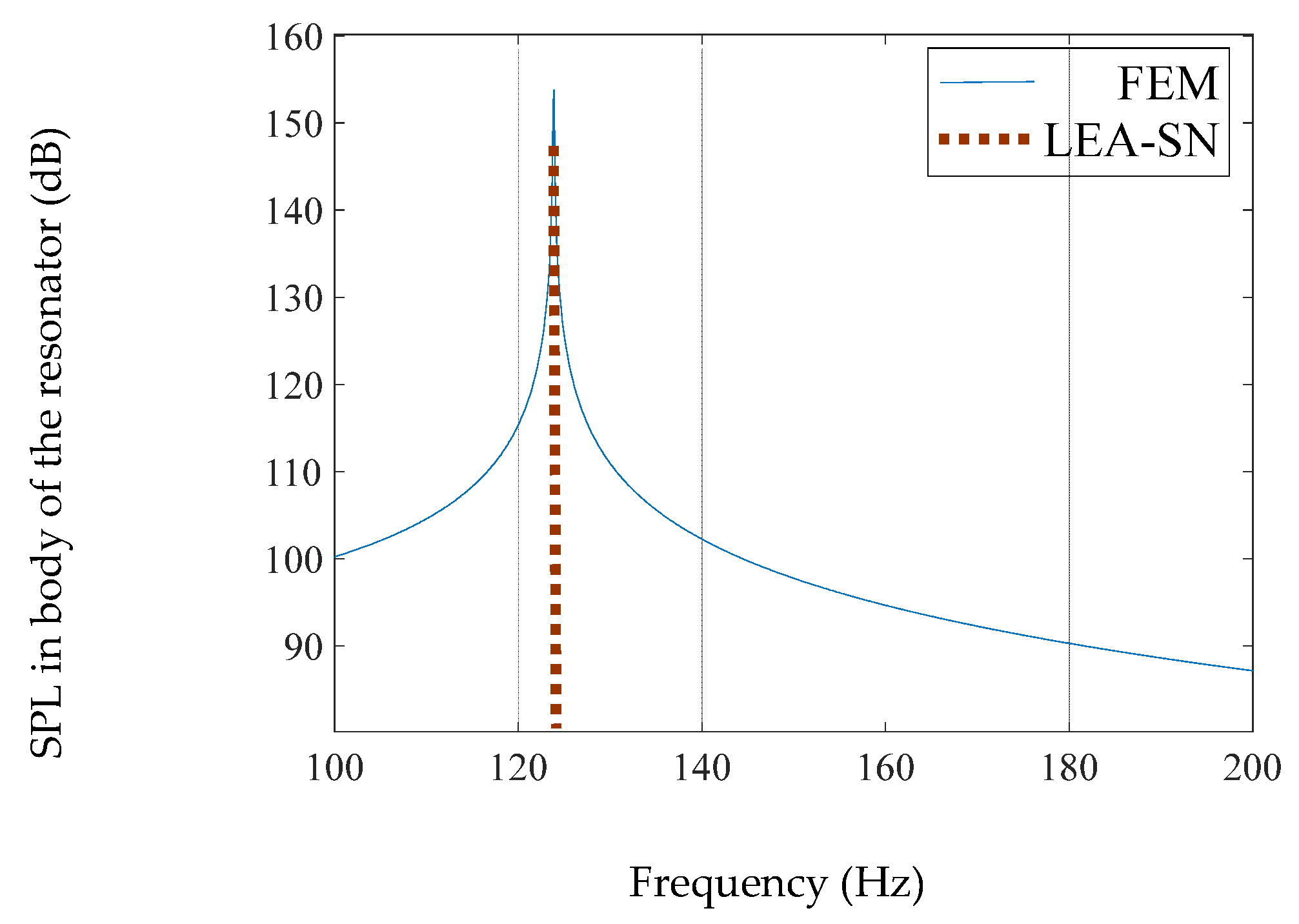
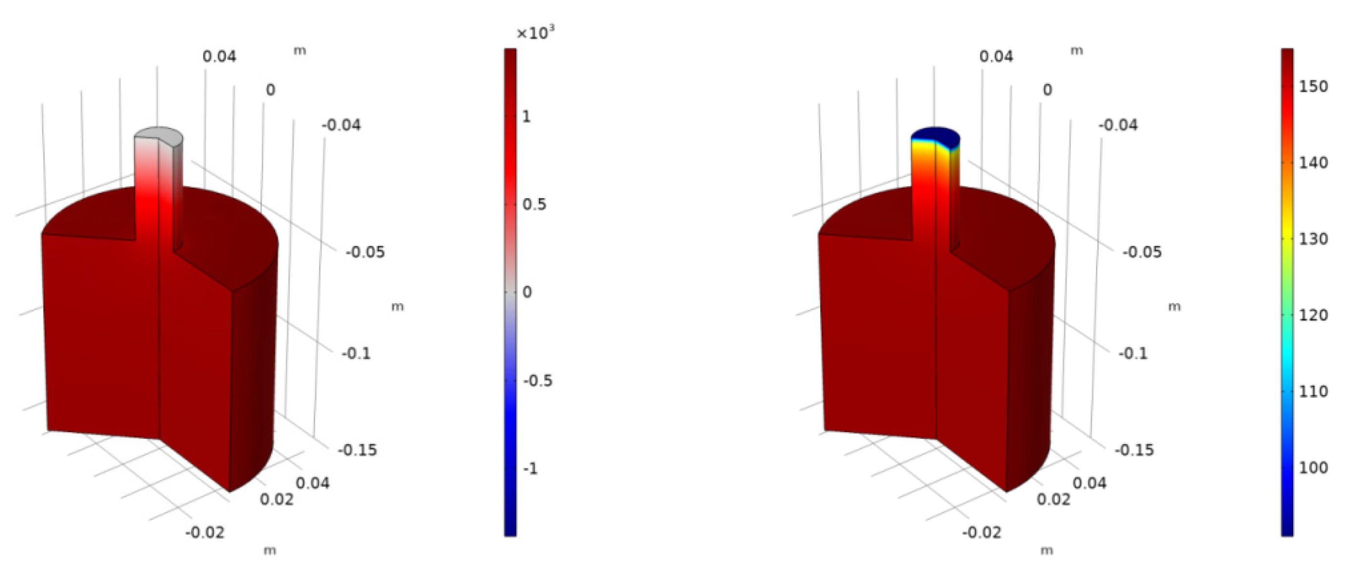
4.1.1. Spherical Body
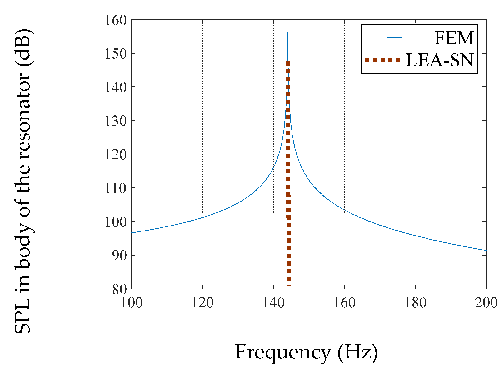
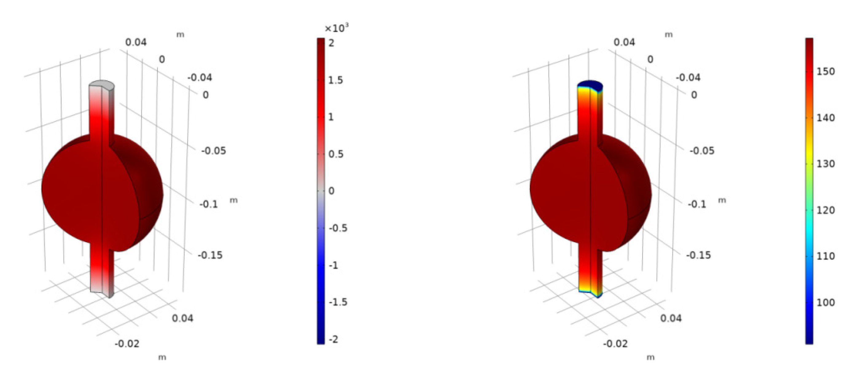
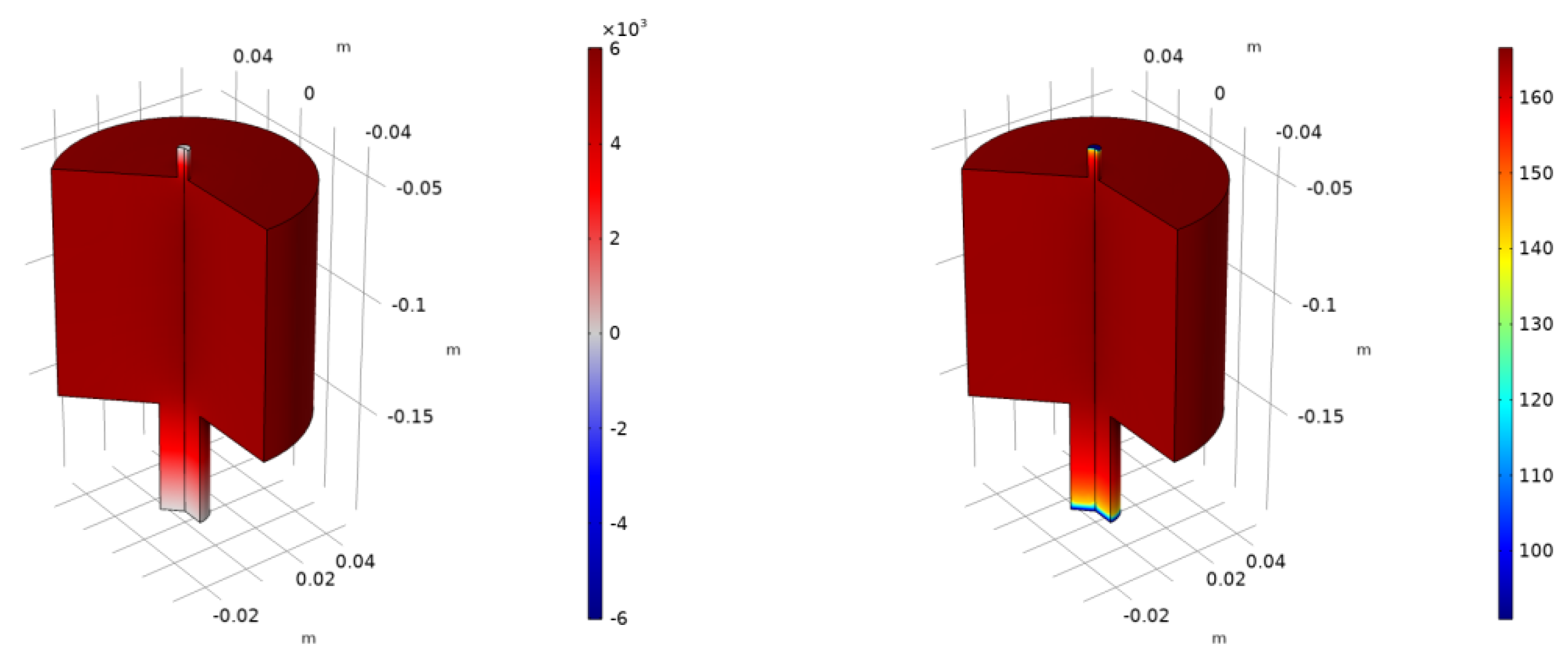
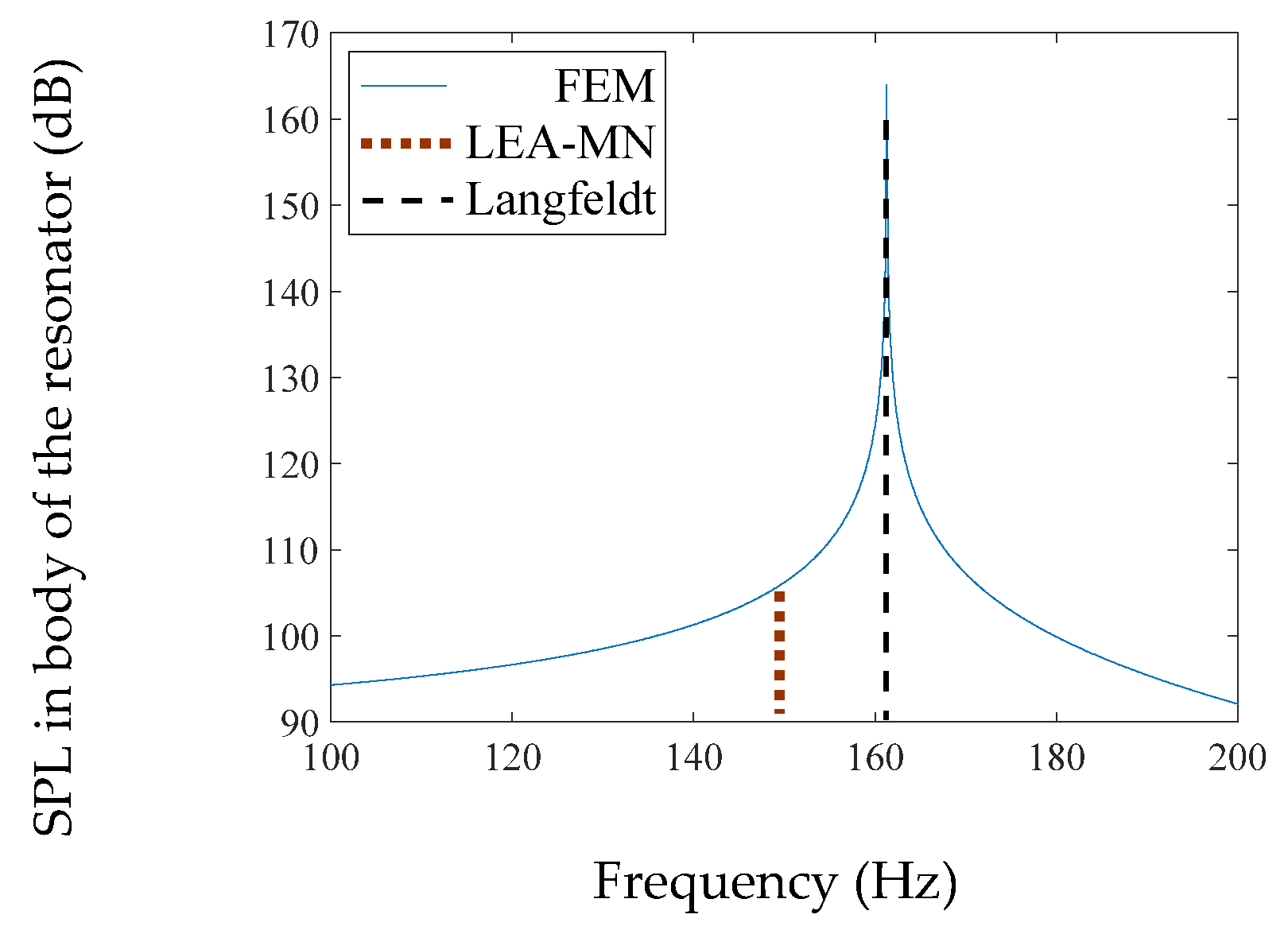
4.1.2. Cylindrical Body
4.2. Multi-Neck Models
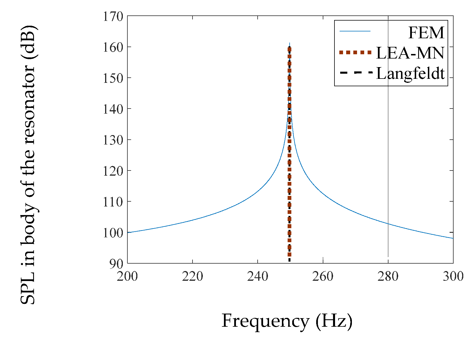
4.2.1. Spherical Body #1 (Identical Necks)
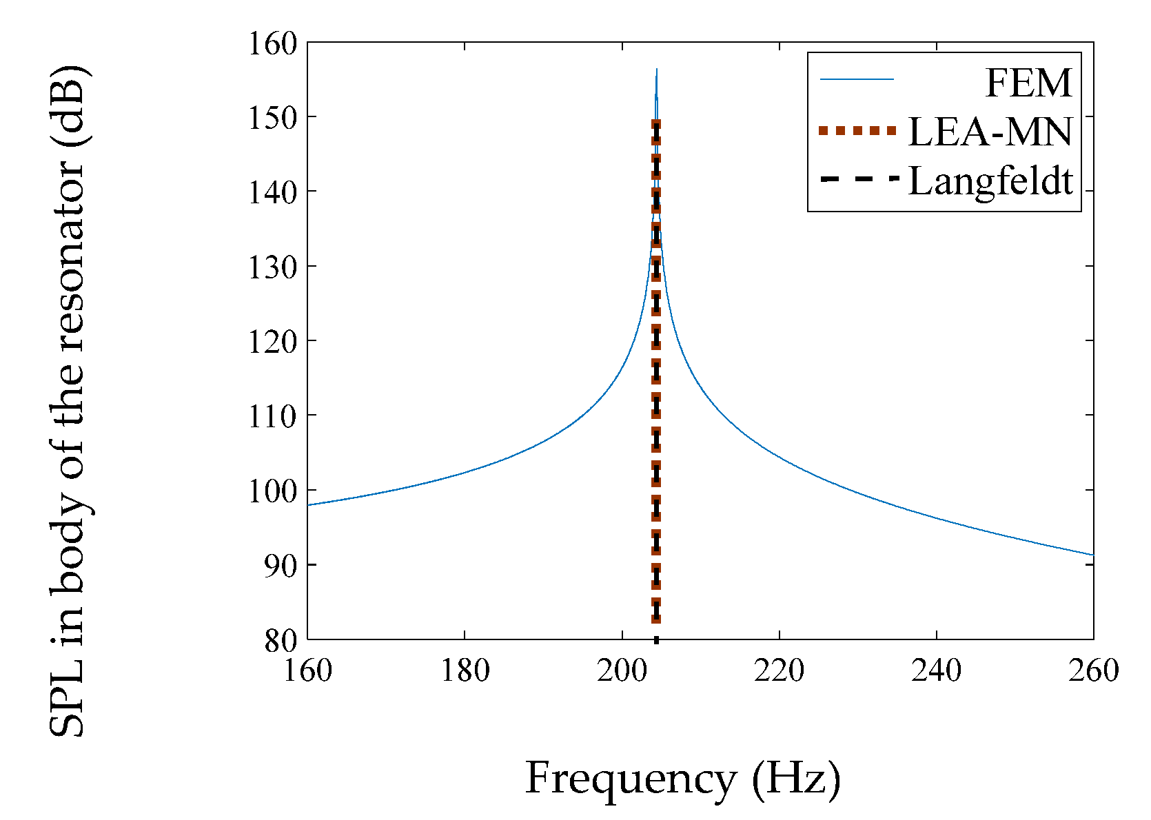
4.2.2. Cylindrical Body #1 (Identical Necks)
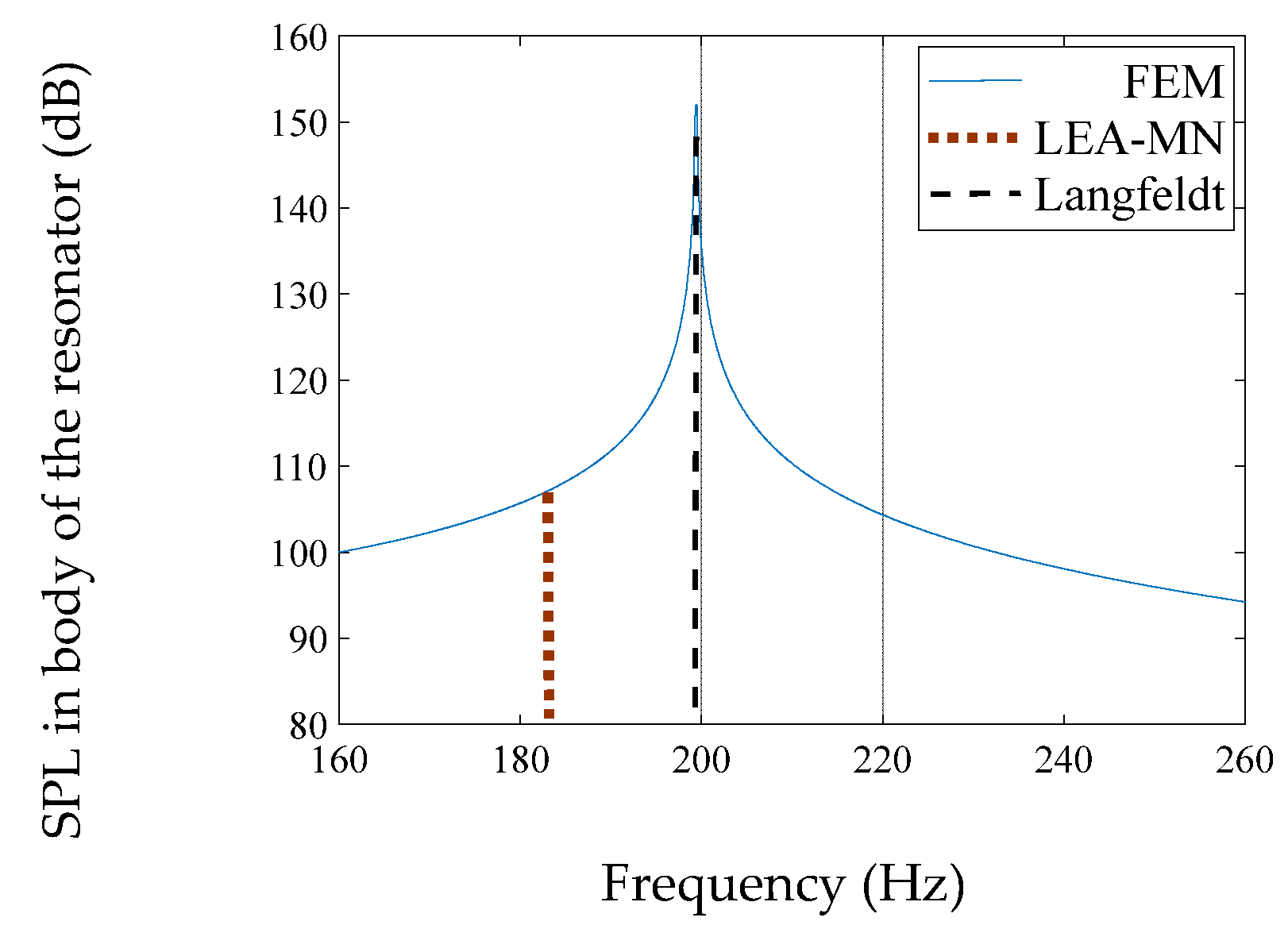
4.2.3. Spherical Body #2 (Different Necks)
4.2.4. Cylindrical Body #2 (Different Necks)
4.2.5. Cylindrical Body #3 (Different Necks, One Flanged Neck)
5. Discussion
6. Conclusions
Author Contributions
Funding
Institutional Review Board Statement
Informed Consent Statement
Data Availability Statement
Conflicts of Interest
References
- Rossing, T.D.; Rossing, T.D. Springer Handbook of Acoustics; Springer: Berlin/Heidelberg, Germany, 2014. [Google Scholar]
- Crocker, M.J.; Price, A.J. Noise and Noise Control: Volume 1; CRC Press: Boca Raton, FL, USA, 2018. [Google Scholar]
- Kone, C.T.; Ghinet, S.; Panneton, R.; Dupont, T.; Grewal, A. Multi-tonal low frequency noise control for aircraft cabin using Helmholtz resonator with complex cavity designs for aircraft cabin noise improvement. In Proceedings of the INTERNOISE-2021, virtually, 1–5 August 2021. [Google Scholar]
- Zhang, Z.; Yu, D.; Liu, J.; Hu, B.; Wen, J. Transmission and bandgap characteristics of a duct mounted with multiple hybrid Helmholtz resonators. Appl. Acoust. 2021, 183, 108266. [Google Scholar] [CrossRef]
- Wu, C.; Chen, L.; Ni, J.; Xu, J. Modeling and experimental verification of a new muffler based on the theory of quarter-wavelength tube and the Helmholtz muffler. SpringerPlus 2016, 5, 1–14. [Google Scholar] [CrossRef] [PubMed]
- Wang, J.; Rubini, P.; Qin, Q.; Houston, B. A model to predict acoustic resonant frequencies of distributed Helmholtz resonators on gas turbine engines. Appl. Sci. 2019, 9, 1419. [Google Scholar] [CrossRef]
- Kanev, N. Maximum sound absorption by a Helmholtz resonator in a room at low frequencies. Acoust. Phys. 2018, 64, 774–777. [Google Scholar] [CrossRef]
- Herrero-Durá, I.; Cebrecos, A.; Picó, R.; Romero-García, V.; García-Raffi, L.M.; Sánchez-Morcillo, V.J. Sound absorption and diffusion by 2D arrays of Helmholtz resonators. Appl. Sci. 2020, 10, 1690. [Google Scholar] [CrossRef]
- Papadakis, N.M.; Stavroulakis, G.E. Review of Acoustic Sources Alternatives to a Dodecahedron Speaker. Appl. Sci. 2019, 9, 3705. [Google Scholar] [CrossRef]
- Papadakis, N.M.; Stavroulakis, G.E. Handclap for Acoustic Measurements: Optimal Application and Limitations. Acoustics 2020, 2, 224–245. [Google Scholar] [CrossRef]
- Papadakis, N.M.; Stavroulakis, G.E. Low Cost Omnidirectional Sound Source Utilizing a Common Directional Loudspeaker for Impulse Response Measurements. Appl. Sci. 2018, 8, 1703. [Google Scholar] [CrossRef]
- Papadakis, N.M.; Antoniadou, S.; Stavroulakis, G.E. Effects of Varying Levels of Background Noise on Room Acoustic Parameters, Measured with ESS and MLS Methods. Acoustics 2023, 5, 563–574. [Google Scholar] [CrossRef]
- Kanev, N. Resonant Vessels in Russian Churches and Their Study in a Concert Hall. In Proceedings of the Acoustics, Virtual, 5–9 October 2020; pp. 399–415. [Google Scholar]
- Pöhlmann, E. Vitruvius De Architectura V: Resounding Vessels in the Greek and Roman Theatre and Their Possible Afterlife in Eastern and Western Churches. Greek Rom. Music. Stud. 2021, 9, 157–174. [Google Scholar] [CrossRef]
- Fredianelli, L.; Del Pizzo, L.G.; Licitra, G. Recent developments in sonic crystals as barriers for road traffic noise mitigation. Environments 2019, 6, 14. [Google Scholar] [CrossRef]
- Castiñeira-Ibañez, S.; Rubio, C.; Sánchez-Pérez, J.V. Environmental noise control during its transmission phase to protect buildings. Design model for acoustic barriers based on arrays of isolated scatterers. Build. Environ. 2015, 93, 179–185. [Google Scholar] [CrossRef]
- Redondo, J.; Ramírez-Solana, D.; Picó, R. Increasing the Insertion Loss of Sonic Crystal Noise Barriers with Helmholtz Resonators. Appl. Sci. 2023, 13, 3662. [Google Scholar] [CrossRef]
- Garcia-Alcaide, V.; Palleja-Cabre, S.; Castilla, R.; Gamez-Montero, P.J.; Romeu, J.; Pamies, T.; Amate, J.; Milán, N. Numerical study of the aerodynamics of sound sources in a bass-reflex port. Eng. Appl. Comput. Fluid Mech. 2017, 11, 210–224. [Google Scholar] [CrossRef]
- Nia, H.T.; Jain, A.D.; Liu, Y.; Alam, M.-R.; Barnas, R.; Makris, N.C. The evolution of air resonance power efficiency in the violin and its ancestors. Proc. R. Soc. A Math. Phys. Eng. Sci. 2015, 471, 20140905. [Google Scholar] [CrossRef]
- Yamamoto, T. Acoustic metamaterial plate embedded with Helmholtz resonators for extraordinary sound transmission loss. J. Appl. Phys. 2018, 123, 215110. [Google Scholar] [CrossRef]
- Casarini, C.; Tiller, B.; Mineo, C.; MacLeod, C.N.; Windmill, J.F.; Jackson, J.C. Enhancing the sound absorption of small-scale 3-D printed acoustic metamaterials based on Helmholtz resonators. IEEE Sens. J. 2018, 18, 7949–7955. [Google Scholar] [CrossRef]
- Yang, X.; Yin, J.; Yu, G.; Peng, L.; Wang, N. Acoustic superlens using Helmholtz-resonator-based metamaterials. Appl. Phys. Lett. 2015, 107, 193505. [Google Scholar] [CrossRef]
- Fang, N.; Xi, D.; Xu, J.; Ambati, M.; Srituravanich, W.; Sun, C.; Zhang, X. Ultrasonic metamaterials with negative modulus. Nat. Mater. 2006, 5, 452–456. [Google Scholar] [CrossRef] [PubMed]
- Ciaburro, G.; Iannace, G. Numerical simulation for the sound absorption properties of ceramic resonators. Fibers 2020, 8, 77. [Google Scholar] [CrossRef]
- Yuan, M.; Cao, Z.; Luo, J.; Chou, X. Recent developments of acoustic energy harvesting: A review. Micromachines 2019, 10, 48. [Google Scholar] [CrossRef]
- Shi, X.; Mak, C.M. Helmholtz resonator with a spiral neck. Appl. Acoust. 2015, 99, 68–71. [Google Scholar] [CrossRef]
- Tang, S.K. On Helmholtz resonators with tapered necks. J. Sound Vib. 2005, 279, 1085–1096. [Google Scholar] [CrossRef]
- Cai, C.; Mak, C.-M.; Shi, X. An extended neck versus a spiral neck of the Helmholtz resonator. Appl. Acoust. 2017, 115, 74–80. [Google Scholar] [CrossRef]
- Ramos, D.; Godinho, L.; Amado-Mendes, P.; Mareze, P. Experimental and numerical modelling of Helmholtz Resonator with angled neck aperture. In Proceedings of the INTER-NOISE and NOISE-CON Congress and Conference Proceedings, Virtual, 16–20 November 2020; pp. 37–47. [Google Scholar]
- Chanaud, R. Effects of geometry on the resonance frequency of Helmholtz resonators, part I. J. Sound Vib. 1994, 178, 337–348. [Google Scholar] [CrossRef]
- Chanaud, R. Effects of geometry on the resonance frequency of Helmholtz resonators, part II. J. Sound Vib. 1997, 204, 829–834. [Google Scholar] [CrossRef]
- Xu, M.; Selamet, A.; Kim, H. Dual helmholtz resonator. Appl. Acoust. 2010, 71, 822–829. [Google Scholar] [CrossRef]
- Langfeldt, F.; Hoppen, H.; Gleine, W. Resonance frequencies and sound absorption of Helmholtz resonators with multiple necks. Appl. Acoust. 2019, 145, 314–319. [Google Scholar] [CrossRef]
- Selamet, A.; Kim, H.; Huff, N.T. Leakage effect in Helmholtz resonators. J. Acoust. Soc. Am. 2009, 126, 1142–1150. [Google Scholar] [CrossRef]
- Lee, I.; Jeon, K.; Park, J. The effect of leakage on the acoustic performance of reactive silencers. Appl. Acoust. 2013, 74, 479–484. [Google Scholar] [CrossRef]
- May, D.; Plotkin, K.; Selden, R.; Sharp, B. Lightweight Sidewalls for Aircraft Interior Noise Control; National Aeronautics and Space Administration: Washington, DC, USA, 1985. [Google Scholar]
- Zolfagharian, A.; Noshadi, A.; Khosravani, M.R.; Zain, M.Z.M. Unwanted noise and vibration control using finite element analysis and artificial intelligence. Appl. Math. Model. 2014, 38, 2435–2453. [Google Scholar] [CrossRef]
- Sakuma, T.; Sakamoto, S.; Otsuru, T. Computational Simulation in Architectural and Environmental Acoustics; Springer: Berlin/Heidelberg, Germany, 2014. [Google Scholar]
- Papadakis, N.M.; Stavroulakis, G.E. Finite Element Method for the Estimation of Insertion Loss of Noise Barriers: Comparison with Various Formulae (2D). Urban Sci. 2020, 4, 77. [Google Scholar] [CrossRef]
- Papadakis, N.M.; Stavroulakis, G.E. Time domain finite element method for the calculation of impulse response of enclosed spaces. Room acoustics application. In Proceedings of the Mechanics of Hearing: Protein to Perception: 12th International Workshop on the Mechanics of Hearing, Cape Sounio, Greece, 31 December 2015; Volume 1703, p. 100002. [Google Scholar] [CrossRef]
- Beranek, L.L.; Mellow, T. Acoustics: Sound Fields and Transducers; Academic Press: Cambridge, MA, USA, 2012. [Google Scholar]
- Ingard, U. Notes on acoustics; Laxmi Publications, Ltd.: Delhi, India, 2010. [Google Scholar]
- Kuttruff, H. Room Acoustics; CRC Press: Boca Raton, FL, USA, 2016. [Google Scholar] [CrossRef]
- Crocker, M.J.; Arenas, J.P. Engineering Acoustics: Noise and Vibration Control; John Wiley & Sons: Hoboken, NJ, USA, 2021. [Google Scholar]
- Marburg, S.; Nolte, B. Computational Acoustics of Noise Propagation in Fluids: Finite and Boundary Element Methods; Springer: Berlin/Heidelberg, Germany, 2008; Volume 578. [Google Scholar]
- Blackstock, D.T. Fundamentals of Physical Acoustics; Wiley: Hoboken, NJ, USA, 2001. [Google Scholar]
- Jena, D.; Dandsena, J.; Jayakumari, V. Demonstration of effective acoustic properties of different configurations of Helmholtz resonators. Appl. Acoust. 2019, 155, 371–382. [Google Scholar] [CrossRef]
- Ihlenburg, F. Finite Element Analysis of Acoustic Scattering; Springer Science & Business Media: Berlin/Heidelberg, Germany, 2006; Volume 132. [Google Scholar]


| Resonant Frequency LEA (Hz) | Resonant Frequency Langfeldt (Hz) | Resonant Frequency FEM (Hz) | Error of Calculation (%) FEM-Langfeldt | Error of Calculation (%) FEM-LEA | |
|---|---|---|---|---|---|
| Single-neck models | |||||
| Spherical | 123.8 | - | 123.7 | - | 0.1 |
| Cylindrical | 144.0 | - | 144.0 | - | 0.0 |
| Multi-neck models | |||||
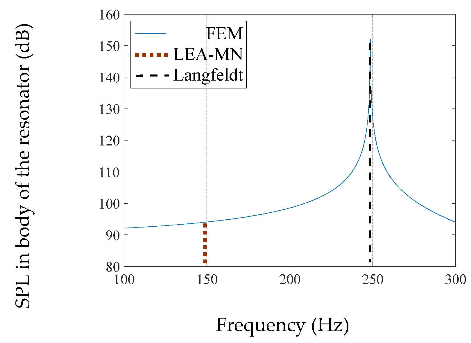
| Spherical #1 | 249.4 | 249.4 | 249.7 | 0.1 | 0.1 |
| Cylindrical #1 | 203.6 | 203.6 | 204.3 | 0.3 | 0.3 |
| Spherical #2 | 181.8 | 197.1 | 199.3 | 1.1 | 8.8 |
| Cylindrical #2 | 148.4 | 161.0 | 161.3 | 0.2 | 8.0 |
| Cylindrical #3 | 148.4 | 245.7 | 248.5 | 1.1 | 40.3 |
Disclaimer/Publisher’s Note: The statements, opinions and data contained in all publications are solely those of the individual author(s) and contributor(s) and not of MDPI and/or the editor(s). MDPI and/or the editor(s) disclaim responsibility for any injury to people or property resulting from any ideas, methods, instructions or products referred to in the content. |
© 2023 by the authors. Licensee MDPI, Basel, Switzerland. This article is an open access article distributed under the terms and conditions of the Creative Commons Attribution (CC BY) license (https://creativecommons.org/licenses/by/4.0/).
Share and Cite
Papadakis, N.M.; Stavroulakis, G.E. FEM Investigation of a Multi-Neck Helmholtz Resonator. Appl. Sci. 2023, 13, 10610. https://doi.org/10.3390/app131910610
Papadakis NM, Stavroulakis GE. FEM Investigation of a Multi-Neck Helmholtz Resonator. Applied Sciences. 2023; 13(19):10610. https://doi.org/10.3390/app131910610
Chicago/Turabian StylePapadakis, Nikolaos M., and Georgios E. Stavroulakis. 2023. "FEM Investigation of a Multi-Neck Helmholtz Resonator" Applied Sciences 13, no. 19: 10610. https://doi.org/10.3390/app131910610
APA StylePapadakis, N. M., & Stavroulakis, G. E. (2023). FEM Investigation of a Multi-Neck Helmholtz Resonator. Applied Sciences, 13(19), 10610. https://doi.org/10.3390/app131910610