


An Improved Cheetah Optimizer for Accurate and Reliable Estimation of Unknown Parameters in Photovoltaic Cell and Module Models


Abstract
:1. Introduction
1.1. Motivation and Incitement
1.2. Literature Review
1.3. Contribution and Paper Organization
- A simplified and improved version of the CO is introduced for parameter estimation of PV models.
- The search phase is controlled according to the leader’s position, and its step length is adjusted following the sorted population. Hence, the proposed search strategy facilitates both global and local search capabilities.
- In the attack phase, the interaction factor is adjusted based on the prey’s position, while the turning factor is determined based on a random value. Using the proposed attack operator, the algorithm is expected to perform better during global searches and achieve faster convergence.
- An extensive study is conducted and compared with other well-established metaheuristic algorithms to evaluate the ICO’s effectiveness.
2. PV Modeling and Problem Formulation
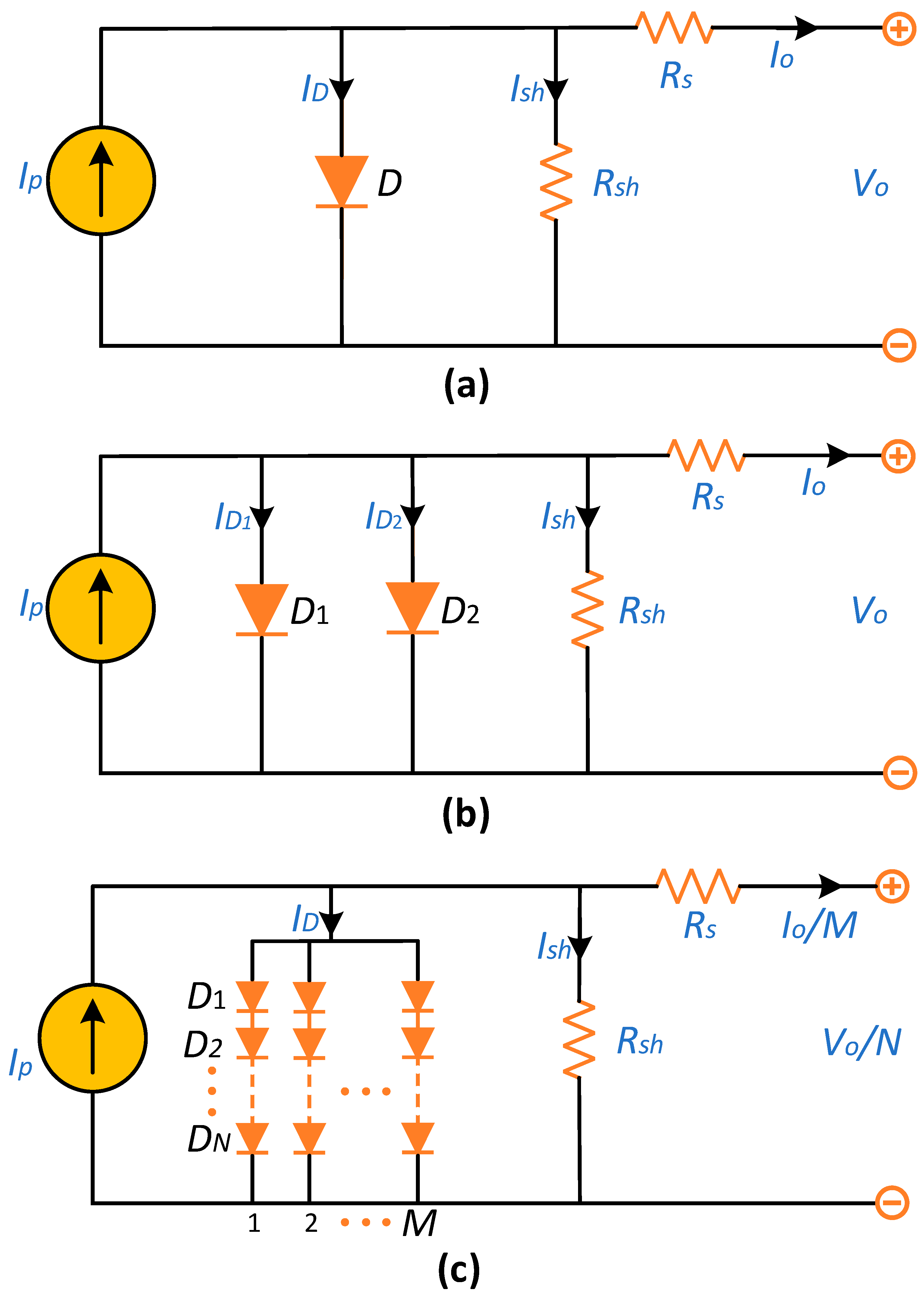
2.1. The Model of a Solar Cell
2.1.1. SDM
2.1.2. DDM
2.2. PVMM
2.3. Problem Formulation
3. Proposed Optimization Algorithm
3.1. Overview of the CO Algorithm
3.1.1. Searching Strategy
3.1.2. Sitting-and-Waiting Strategy
3.1.3. Attacking Strategy
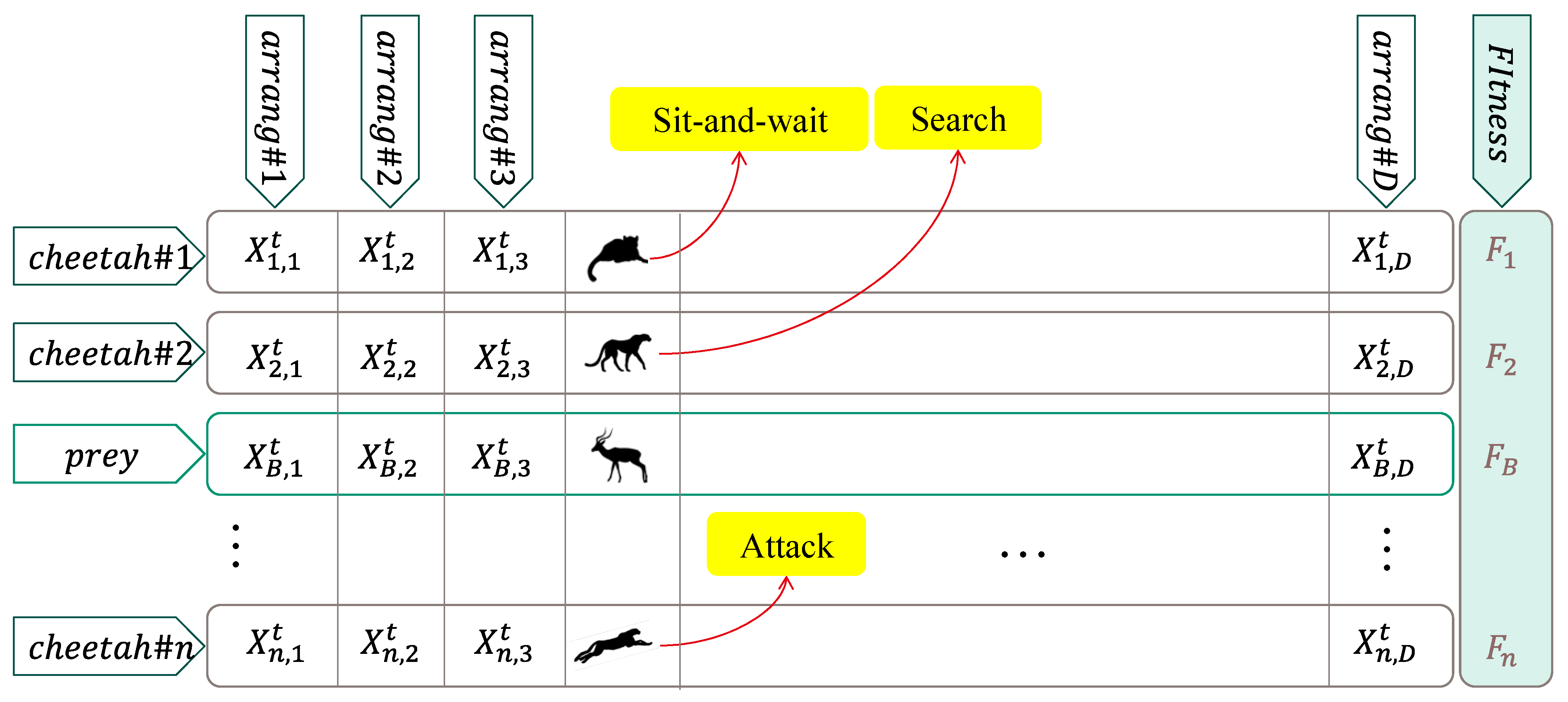
3.1.4. Strategy Selection Mechanism
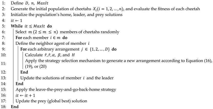
| Algorithm 1. The CO Algorithm |
 |
3.2. Improved Cheetah Optimizer (ICO) Algorithm
3.2.1. Searching Strategy
3.2.2. Attacking Strategy
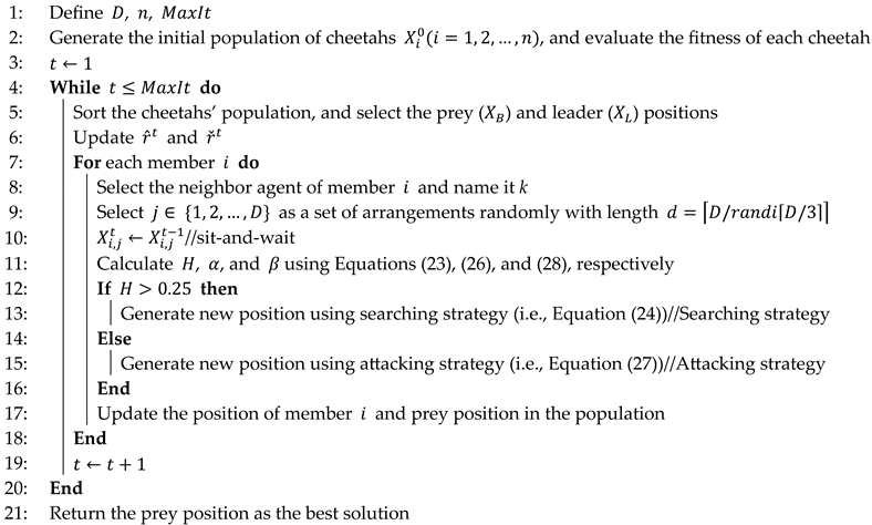
| Algorithm 2. The ICO Algorithm |
 |
4. Experimental Results
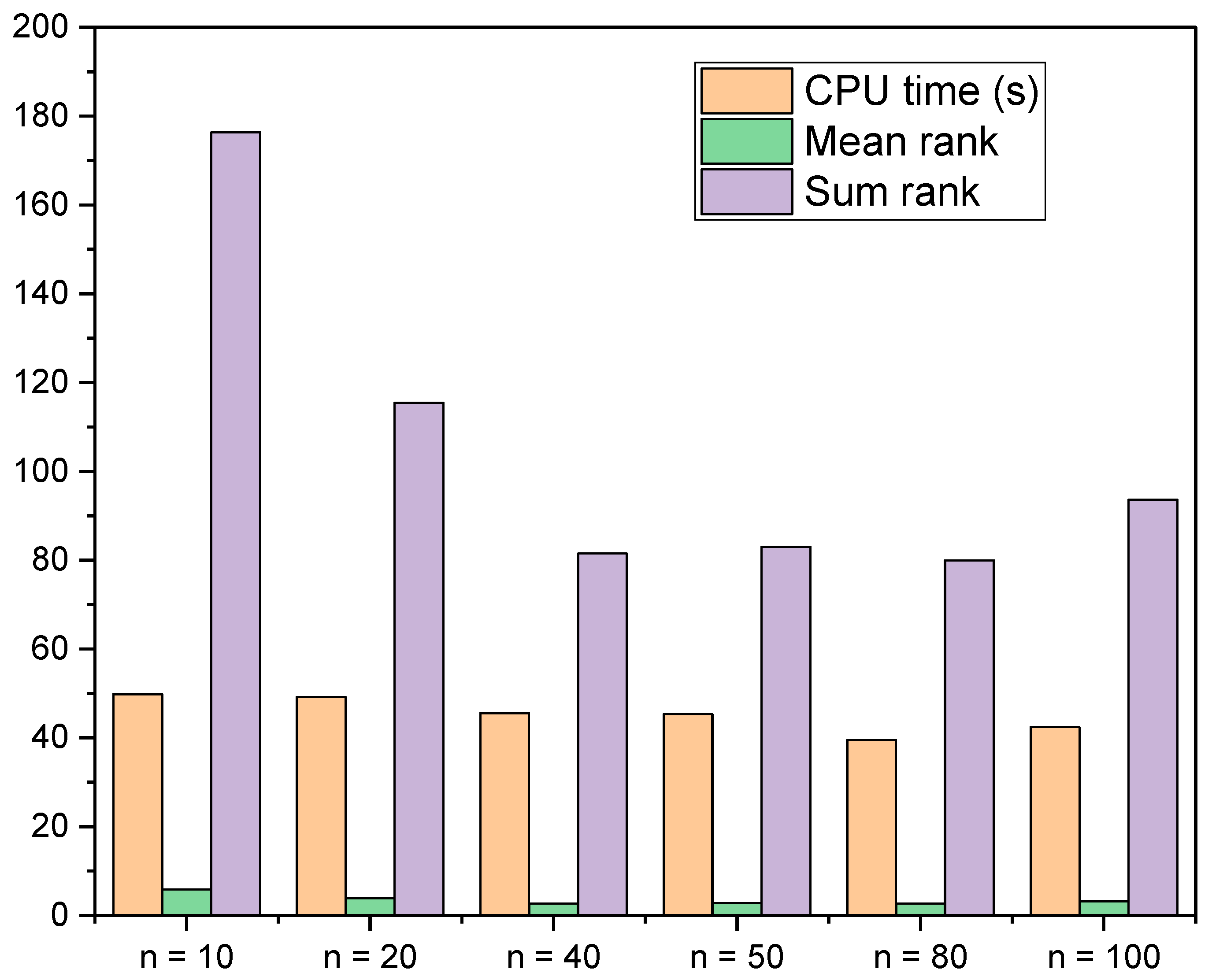
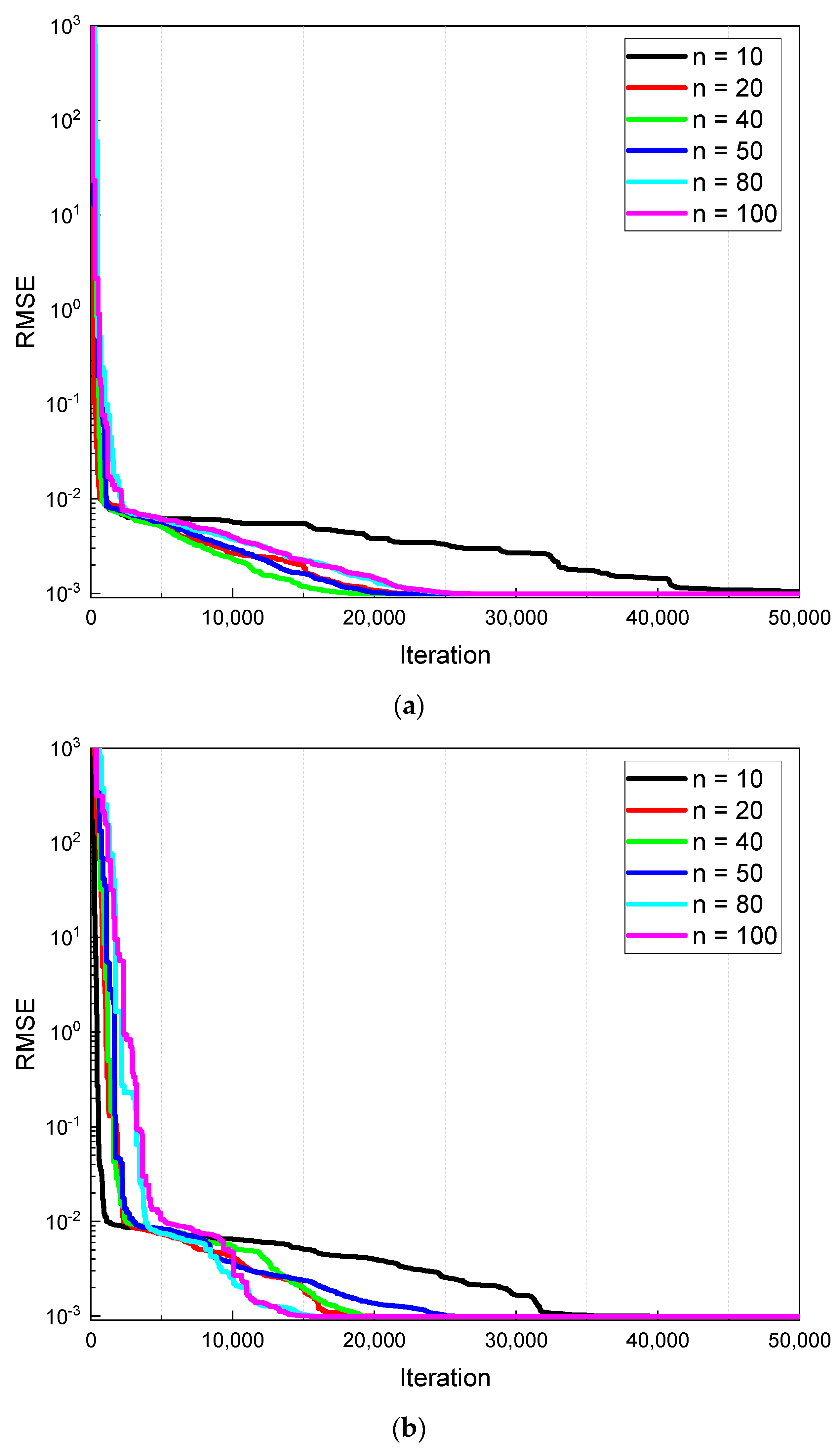
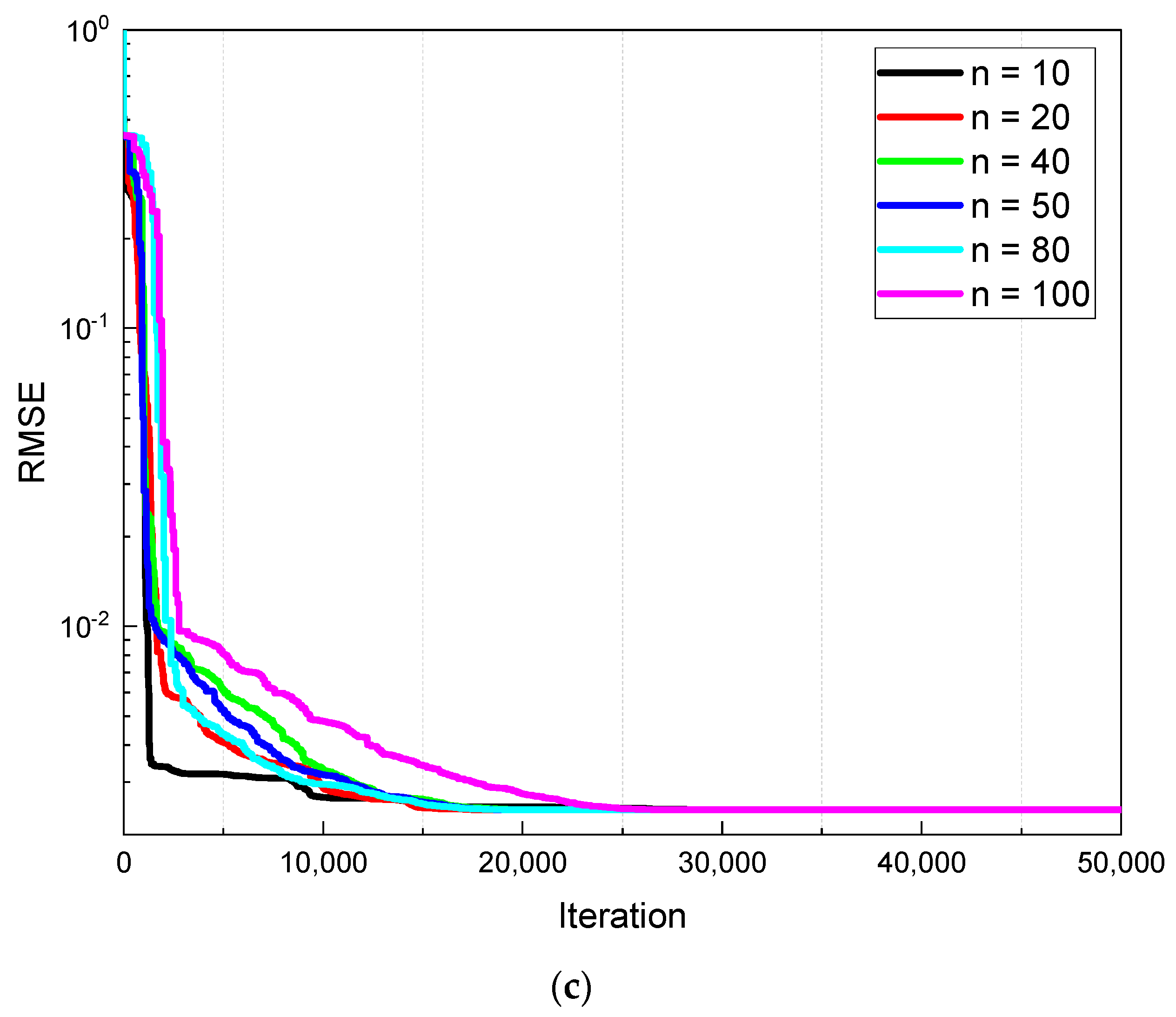
4.1. Population Size Analysis
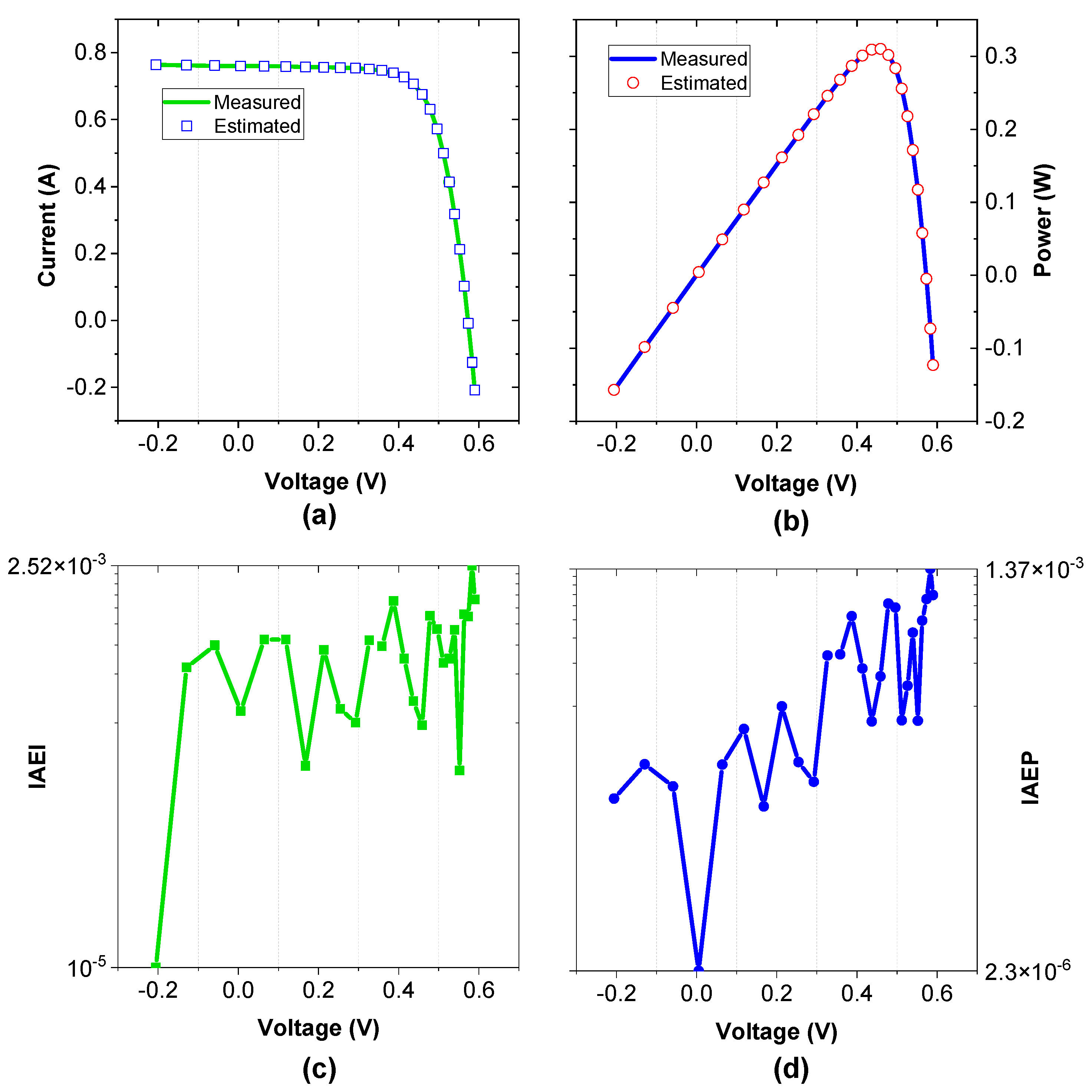
4.2. Results of Parameter Extraction Based on the SDM
4.3. Results of Parameter Extraction Based on the DDM
4.4. PVMM-Based Photo Watt-PWP 201
4.5. Comparison of Statistical Results
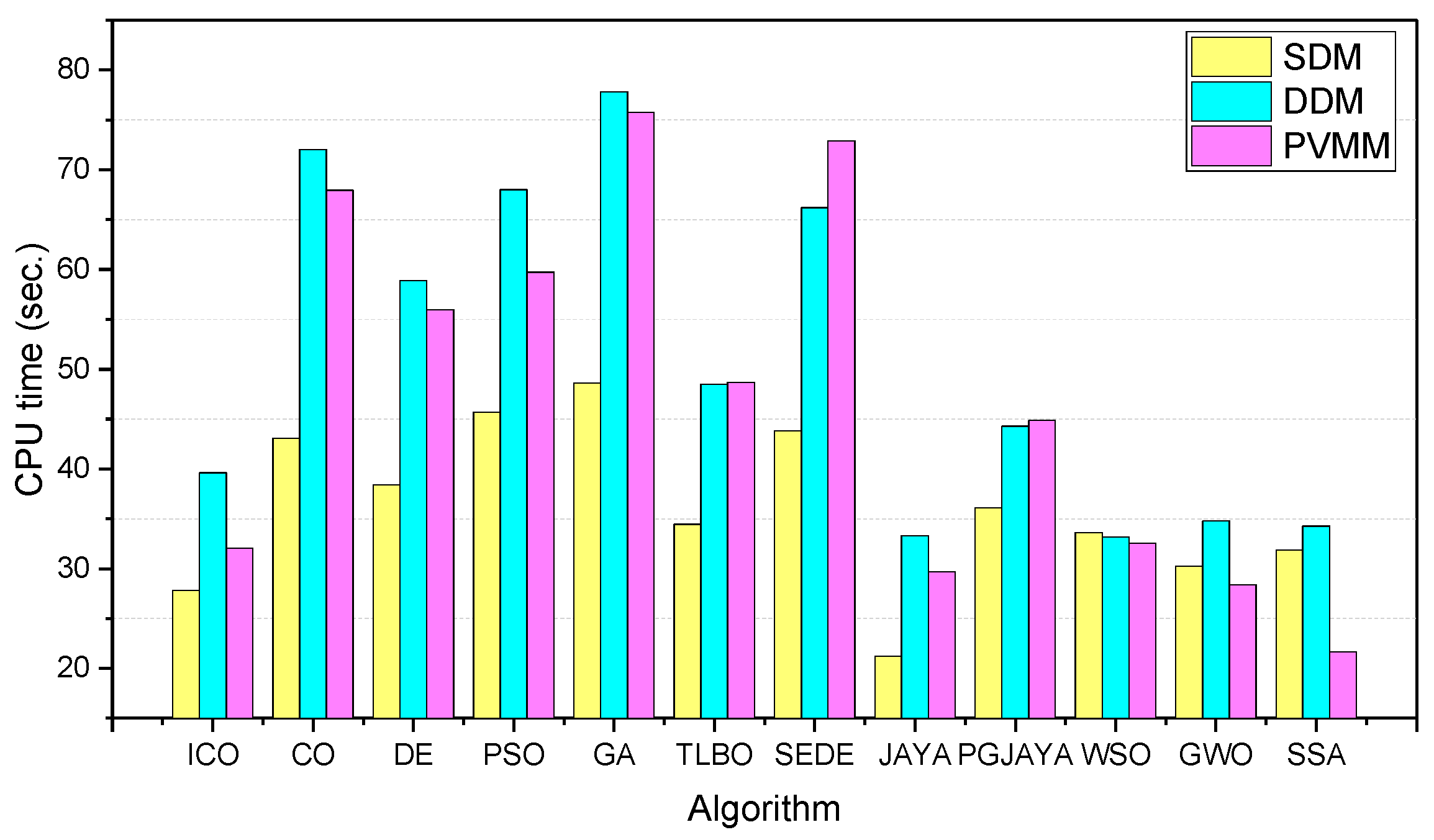
4.6. Computational Time
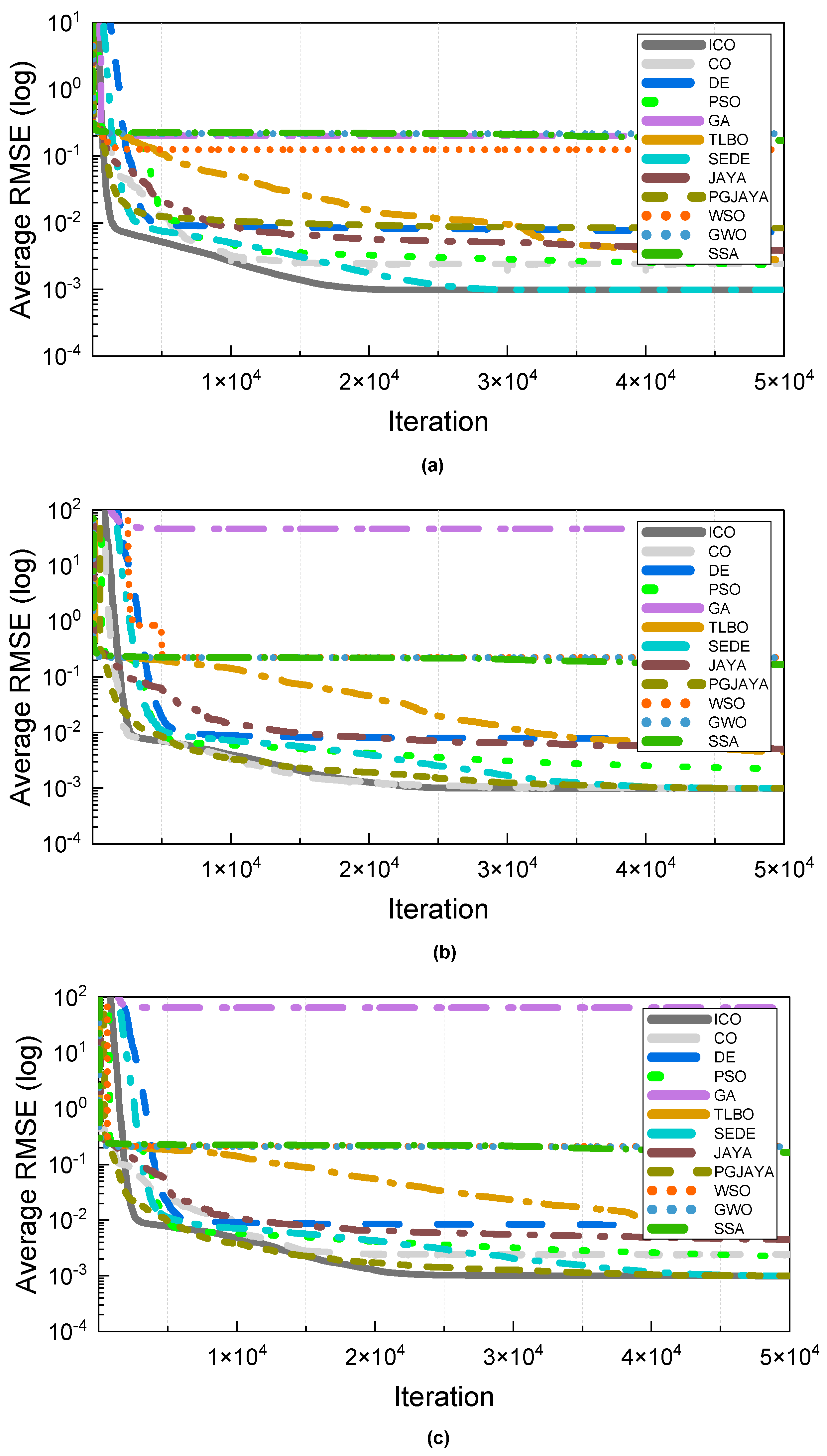
4.7. Convergence Characteristics
4.8. Exploration and Exploitation Analysis
4.9. Results for STM6-40/36 PV Module
4.10. Comparison with the State-of-the-Art Methods
5. Conclusions
Author Contributions
Funding
Institutional Review Board Statement
Informed Consent Statement
Data Availability Statement
Conflicts of Interest
References
- Sheng, R.; Du, J.; Liu, S.; Wang, C.; Wang, Z.; Liu, X. Solar Photovoltaic Investment Changes across China Regions Using a Spatial Shift-Share Analysis. Energies 2021, 14, 6418. [Google Scholar] [CrossRef]
- Chen, H.; Jiao, S.; Heidari, A.A.; Wang, M.; Chen, X.; Zhao, X. An Opposition-Based Sine Cosine Approach with Local Search for Parameter Estimation of Photovoltaic Models. Energy Convers. Manag. 2019, 195, 927–942. [Google Scholar] [CrossRef]
- Jiang, L.L.; Maskell, D.L.; Patra, J.C. Parameter Estimation of Solar Cells and Modules Using an Improved Adaptive Differential Evolution Algorithm. Appl. Energy 2013, 112, 185–193. [Google Scholar] [CrossRef]
- Rasheduzzaman, M.; Fajri, P.; Kimball, J.; Deken, B. Modeling, Analysis, and Control Design of a Single-Stage Boost Inverter. Energies 2021, 14, 4098. [Google Scholar] [CrossRef]
- Yu, K.; Chen, X.; Wang, X.; Wang, Z. Parameters Identification of Photovoltaic Models Using Self-Adaptive Teaching-Learning-Based Optimization. Energy Convers. Manag. 2017, 145, 233–246. [Google Scholar] [CrossRef]
- Yu, K.; Qu, B.; Yue, C.; Ge, S.; Chen, X.; Liang, J. A Performance-Guided JAYA Algorithm for Parameters Identification of Photovoltaic Cell and Module. Appl. Energy 2019, 237, 241–257. [Google Scholar] [CrossRef]
- Mehta, H.K.; Warke, H.; Kukadiya, K.; Panchal, A.K. Accurate Expressions for Single-Diode-Model Solar Cell Parameterization. IEEE J. Photovolt. 2019, 9, 803–810. [Google Scholar] [CrossRef]
- Hejri, M.; Mokhtari, H.; Azizian, M.R.; Ghandhari, M.; Söder, L. On the Parameter Extraction of a Five-Parameter Double-Diode Model of Photovoltaic Cells and Modules. IEEE J. Photovolt. 2014, 4, 915–923. [Google Scholar] [CrossRef]
- Chin, V.J.; Salam, Z. A New Three-Point-Based Approach for the Parameter Extraction of Photovoltaic Cells. Appl. Energy 2019, 237, 519–533. [Google Scholar] [CrossRef]
- Ishaque, K.; Salam, Z. An Improved Modeling Method to Determine the Model Parameters of Photovoltaic (PV) Modules Using Differential Evolution (DE). Sol. Energy 2011, 85, 2349–2359. [Google Scholar] [CrossRef]
- Dali, A.; Bouharchouche, A.; Diaf, S. Parameter Identification of Photovoltaic Cell/Module Using Genetic Algorithm (GA) and Particle Swarm Optimization (PSO). In Proceedings of the 2015 3rd International Conference on Control, Engineering & Information Technology (CEIT), Tlemcen, Algeria, 25–27 May 2015; IEEE: New York, NY, USA, 2015; pp. 1–6. [Google Scholar]
- Khanna, V.; Das, B.K.; Bisht, D.; Singh, P.K. A Three Diode Model for Industrial Solar Cells and Estimation of Solar Cell Parameters Using PSO Algorithm. Renew. Energy 2015, 78, 105–113. [Google Scholar] [CrossRef]
- Ayyarao, T.S.; Kumar, P.P. Parameter Estimation of Solar PV Models with a New Proposed War Strategy Optimization Algorithm. Int. J. Energy Res. 2022, 46, 7215–7238. [Google Scholar] [CrossRef]
- Liang, J.; Qiao, K.; Yu, K.; Ge, S.; Qu, B.; Xu, R.; Li, K. Parameters Estimation of Solar Photovoltaic Models via a Self-Adaptive Ensemble-Based Differential Evolution. Sol. Energy 2020, 207, 336–346. [Google Scholar] [CrossRef]
- Abbassi, R.; Abbassi, A.; Heidari, A.A.; Mirjalili, S. An Efficient Salp Swarm-Inspired Algorithm for Parameters Identification of Photovoltaic Cell Models. Energy Convers. Manag. 2019, 179, 362–372. [Google Scholar] [CrossRef]
- Yu, K.; Liang, J.J.; Qu, B.Y.; Chen, X.; Wang, H. Parameters Identification of Photovoltaic Models Using an Improved JAYA Optimization Algorithm. Energy Convers. Manag. 2017, 150, 742–753. [Google Scholar] [CrossRef]
- Premkumar, M.; Babu, T.S.; Umashankar, S.; Sowmya, R. A New Metaphor-Less Algorithms for the Photovoltaic Cell Parameter Estimation. Optik 2020, 208, 164559. [Google Scholar] [CrossRef]
- Jamadi, M.; Merrikh-Bayat, F.; Bigdeli, M. Very Accurate Parameter Estimation of Single-and Double-Diode Solar Cell Models Using a Modified Artificial Bee Colony Algorithm. Int. J. Energy Environ. Eng. 2016, 7, 13–25. [Google Scholar] [CrossRef]
- Sheng, H.; Li, C.; Wang, H.; Yan, Z.; Xiong, Y.; Cao, Z.; Kuang, Q. Parameters Extraction of Photovoltaic Models Using an Improved Moth-Flame Optimization. Energies 2019, 12, 3527. [Google Scholar] [CrossRef]
- Hasanien, H.M. Shuffled Frog Leaping Algorithm for Photovoltaic Model Identification. IEEE Trans. Sustain. Energy 2015, 6, 509–515. [Google Scholar] [CrossRef]
- Liao, Z.; Chen, Z.; Li, S. Parameters Extraction of Photovoltaic Models Using Triple-Phase Teaching-Learning-Based Optimization. IEEE Access 2020, 8, 69937–69952. [Google Scholar] [CrossRef]
- Oliva, D.; Abd El Aziz, M.; Hassanien, A.E. Parameter Estimation of Photovoltaic Cells Using an Improved Chaotic Whale Optimization Algorithm. Appl. Energy 2017, 200, 141–154. [Google Scholar] [CrossRef]
- Montoya, O.D.; Gil-González, W.; Grisales-Noreña, L.F. Sine-Cosine Algorithm for Parameters’ Estimation in Solar Cells Using Datasheet Information. In Proceedings of the Journal of Physics: Conference Series; IOP Publishing: Bristol, UK, 2020; Volume 1671, p. 12008. [Google Scholar]
- Long, W.; Cai, S.; Jiao, J.; Xu, M.; Wu, T. A New Hybrid Algorithm Based on Grey Wolf Optimizer and Cuckoo Search for Parameter Extraction of Solar Photovoltaic Models. Energy Convers. Manag. 2020, 203, 112243. [Google Scholar]
- Diab, A.A.Z.; Sultan, H.M.; Do, T.D.; Kamel, O.M.; Mossa, M.A. Coyote Optimization Algorithm for Parameters Estimation of Various Models of Solar Cells and PV Modules. IEEE Access 2020, 8, 111102–111140. [Google Scholar] [CrossRef]
- Soliman, M.A.; Hasanien, H.M.; Alkuhayli, A. Marine Predators Algorithm for Parameters Identification of Triple-Diode Photovoltaic Models. IEEE Access 2020, 8, 155832–155842. [Google Scholar] [CrossRef]
- Kumari, P.A.; Geethanjali, P. Adaptive Genetic Algorithm Based Multi-Objective Optimization for Photovoltaic Cell Design Parameter Extraction. Energy Procedia 2017, 117, 432–441. [Google Scholar] [CrossRef]
- Abdel-Basset, M.; Mohamed, R.; Mirjalili, S.; Chakrabortty, R.K.; Ryan, M.J. Solar Photovoltaic Parameter Estimation Using an Improved Equilibrium Optimizer. Sol. Energy 2020, 209, 694–708. [Google Scholar] [CrossRef]
- Kumar, C.; Raj, T.D.; Premkumar, M.; Raj, T.D. A New Stochastic Slime Mould Optimization Algorithm for the Estimation of Solar Photovoltaic Cell Parameters. Optik 2020, 223, 165277. [Google Scholar] [CrossRef]
- Jiao, S.; Chong, G.; Huang, C.; Hu, H.; Wang, M.; Heidari, A.A.; Chen, H.; Zhao, X. Orthogonally Adapted Harris Hawks Optimization for Parameter Estimation of Photovoltaic Models. Energy 2020, 203, 117804. [Google Scholar] [CrossRef]
- Wolpert, D.H.; Macready, W.G. No Free Lunch Theorems for Optimization. IEEE Trans. Evol. Comput. 1997, 1, 67–82. [Google Scholar] [CrossRef]
- Akbari, M.A.; Zare, M.; Azizipanah-Abarghooee, R.; Mirjalili, S.; Deriche, M. The Cheetah Optimizer: A Nature-Inspired Metaheuristic Algorithm for Large-Scale Optimization Problems. Sci. Rep. 2022, 12, 10953. [Google Scholar] [CrossRef]
- Storn, R.; Price, K. Differential Evolution--a Simple and Efficient Heuristic for Global Optimization over Continuous Spaces. J. Glob. Optim. 1997, 11, 341–359. [Google Scholar] [CrossRef]
- Kennedy, J.; Eberhart, R. Particle Swarm Optimization. In Proceedings of the ICNN’95-International Conference On Neural Networks, Perth, WA, Australia, 27 November–1 December 1995; IEEE: New York, NY, USA, 1995; Volume 4, pp. 1942–1948. [Google Scholar]
- Mitchell, M. An Introduction to Genetic Algorithms; MIT Press: Cambridge, MA, USA, 1998. [Google Scholar]
- Rao, R.V.; Savsani, V.J.; Vakharia, D.P. Teaching–Learning-Based Optimization: An Optimization Method for Continuous Non-Linear Large Scale Problems. Inf. Sci. 2012, 183, 1–15. [Google Scholar] [CrossRef]
- Rao, R. Jaya: A Simple and New Optimization Algorithm for Solving Constrained and Unconstrained Optimization Problems. Int. J. Ind. Eng. Comput. 2016, 7, 19–34. [Google Scholar] [CrossRef]
- Mirjalili, S.; Gandomi, A.H.; Mirjalili, S.Z.; Saremi, S.; Faris, H.; Mirjalili, S.M. Salp Swarm Algorithm: A Bio-Inspired Optimizer for Engineering Design Problems. Adv. Eng. Softw. 2017, 114, 163–191. [Google Scholar] [CrossRef]
- Mirjalili, S.; Mirjalili, S.M.; Lewis, A. Grey Wolf Optimizer. Adv. Eng. Softw. 2014, 69, 46–61. [Google Scholar] [CrossRef]
- AlRashidi, M.R.; AlHajri, M.F.; El-Naggar, K.M.; Al-Othman, A.K. A New Estimation Approach for Determining the I–V Characteristics of Solar Cells. Sol. Energy 2011, 85, 1543–1550. [Google Scholar] [CrossRef]
- Easwarakhanthan, T.; Bottin, J.; Bouhouch, I.; Boutrit, C. Nonlinear Minimization Algorithm for Determining the Solar Cell Parameters with Microcomputers. Int. J. Sol. Energy 1986, 4, 1–12. [Google Scholar] [CrossRef]
- Hussain, K.; Salleh, M.N.M.; Cheng, S.; Shi, Y. On the Exploration and Exploitation in Popular Swarm-Based Metaheuristic Algorithms. Neural Comput. Appl. 2019, 31, 7665–7683. [Google Scholar] [CrossRef]
- El-Sehiemy, R.; Shaheen, A.; El-Fergany, A.; Ginidi, A. Electrical Parameters Extraction of PV Modules Using Artificial Hummingbird Optimizer. Sci. Rep. 2023, 13, 9240. [Google Scholar] [CrossRef]
- Tong, N.T.; Pora, W. A Parameter Extraction Technique Exploiting Intrinsic Properties of Solar Cells. Appl. Energy 2016, 176, 104–115. [Google Scholar] [CrossRef]
- Abdollahzadeh, B.; Gharehchopogh, F.S.; Mirjalili, S. African Vultures Optimization Algorithm: A New Nature-Inspired Metaheuristic Algorithm for Global Optimization Problems. Comput. Ind. Eng. 2021, 158, 107408. [Google Scholar] [CrossRef]
- Xie, L.; Han, T.; Zhou, H.; Zhang, Z.-R.; Han, B.; Tang, A. Tuna Swarm Optimization: A Novel Swarm-Based Metaheuristic Algorithm for Global Optimization. Comput. Intell. Neurosci. 2021, 2021, 9210050. [Google Scholar] [CrossRef]
- Eslami, M.; Akbari, E.; Seyed Sadr, S.T.; Ibrahim, B.F. A Novel Hybrid Algorithm Based on Rat Swarm Optimization and Pattern Search for Parameter Extraction of Solar Photovoltaic Models. Energy Sci. Eng. 2022, 10, 2689–2713. [Google Scholar] [CrossRef]
- Alanazi, M.; Alanazi, A.; Almadhor, A.; Rauf, H.T. Photovoltaic Models’ Parameter Extraction Using New Artificial Parameterless Optimization Algorithm. Mathematics 2022, 10, 4617. [Google Scholar] [CrossRef]
- Chen, X.; Tianfield, H.; Du, W.; Liu, G. Biogeography-Based Optimization with Covariance Matrix Based Migration. Appl. Soft Comput. 2016, 45, 71–85. [Google Scholar] [CrossRef]
- Gong, W.; Cai, Z.; Ling, C.X. DE/BBO: A Hybrid Differential Evolution with Biogeography-Based Optimization for Global Numerical Optimization. Soft Comput. 2010, 15, 645–665. [Google Scholar] [CrossRef]
- Chen, X.; Tianfield, H.; Mei, C.; Du, W.; Liu, G. Biogeography-Based Learning Particle Swarm Optimization. Soft Comput. 2017, 21, 7519–7541. [Google Scholar] [CrossRef]
- Liang, J.J.; Qin, A.K.; Suganthan, P.N.; Baskar, S. Comprehensive Learning Particle Swarm Optimizer for Global Optimization of Multimodal Functions. IEEE Trans. Evol. Comput. 2006, 10, 281–295. [Google Scholar] [CrossRef]
- Yaghoubi, M.; Eslami, M.; Noroozi, M.; Mohammadi, H.; Kamari, O.; Palani, S. Modified Salp Swarm Optimization for Parameter Estimation of Solar PV Models. IEEE Access 2022, 10, 110181–110194. [Google Scholar] [CrossRef]
- Chen, X.; Xu, B.; Mei, C.; Ding, Y.; Li, K. Teaching–Learning–Based Artificial Bee Colony for Solar Photovoltaic Parameter Estimation. Appl. Energy 2018, 212, 1578–1588. [Google Scholar] [CrossRef]
- Chen, X.; Yu, K.; Du, W.; Zhao, W.; Liu, G. Parameters Identification of Solar Cell Models Using Generalized Oppositional Teaching Learning Based Optimization. Energy 2016, 99, 170–180. [Google Scholar] [CrossRef]
- Niu, Q.; Zhang, H.; Li, K. An Improved TLBO with Elite Strategy for Parameters Identification of PEM Fuel Cell and Solar Cell Models. Int. J. Hydrogen Energy 2014, 39, 3837–3854. [Google Scholar] [CrossRef]
- Fathy, A.; Rezk, H. Multi-Verse Optimizer for Identifying the Optimal Parameters of PEMFC Model. Energy 2018, 143, 634–644. [Google Scholar] [CrossRef]
- Sayed, G.I.; Darwish, A.; Hassanien, A.E. Quantum Multiverse Optimization Algorithm for Optimization Problems. Neural Comput. Appl. 2019, 31, 2763–2780. [Google Scholar] [CrossRef]
- Gong, W.; Cai, Z. Parameter Extraction of Solar Cell Models Using Repaired Adaptive Differential Evolution. Sol. Energy 2013, 94, 209–220. [Google Scholar] [CrossRef]
- Xiong, G.; Zhang, J.; Shi, D.; He, Y. Parameter Extraction of Solar Photovoltaic Models Using an Improved Whale Optimization Algorithm. Energy Convers. Manag. 2018, 174, 388–405. [Google Scholar] [CrossRef]


| Algorithm | PV Type | PV Model | Disadvantage | Advantage |
|---|---|---|---|---|
| PGJAYA [6] | RTC France Si cell and PhotoWatt-PWP201 | SDM, DDM, PVMM | Insufficient reliability | Acceptable accuracy |
| DE [10] | SM55 module | SDM | The parameters need to be adjusted and insufficient capability for exploitation | Accurate performance under a variety of operating conditions |
| Possessing good exploration capabilities | ||||
| PSO [12] | Not specified | SDM, DDM | Stuck in local minima and convergence at the beginning | High level of accuracy in the solution |
| Ease of implementation | ||||
| Robustness | ||||
| SEDE [14] | RTC France Si cell and PhotoWatt-PWP201 | SDM, DDM, PVMM | High computation time | High accuracy and robustness |
| WSO [13] | RTC France silicon solar cell, Photo watt-PWP 201, and STM6-40/36 PV modules | SDM, DDM, PVMM | Insufficient robustness | New optimization algorithm for parameter extraction of PV cells and modules and low CPU time |
| SSA [15] | TITAN-12-50 | DDM | Caught within local minimums, and convergence occurs early in the process | Low computational time |
| IJAYA [16] | RTC France Si cell | SDM, DDM | Caught by local minima and inaccurate solution | A simpler and more efficient algorithm |
| Convergence and robustness are high | ||||
| Rao [17] | RTC France Si cell and PhotoWatt-PWP201 | SDM, DDM | Stuck in local minima, and commercial modules have not been tested | Ease of implementation |
| The ability to explore well | ||||
| MABC [18] | RTC France Si cell | SDM, DDM | Excessive computation time | High accuracy and robustness |
| Parameters need to be adjusted frequently and achieving convergence early | Insensitive to noise | |||
| IMFO [19] | Q6-1380 solar cell and CS6P-240P module | SDM, DDM | It takes a long time to compute, and commercial modules have not been tested | Convergence speed is high, and it is simpler |
| SFLA [20] | KC200GT and MSX-60 | SDM | Not accurate | Fast convergence |
| A lot of control parameters | ||||
| TPTLBO [21] | RTC France Si cell | SDM, DDM | High computational costs and uncertainty about the solution | Ease of implementation |
| Fewer control parameters | ||||
| Fast convergence | ||||
| ICWO [22] | KC200GT | SDM, DDM | Inability to explore, caught within local minimums, and convergence occurs early in the process | Easily implemented and a lower cost of computation |
| Capacity for fair exploitation | ||||
| SCA [23] | KC200GT | SDM | KC200GT module only tested and a local minimum trap | Easy to implement and simple to use, with a fair degree of accuracy |
| GWO-CS [24] | KC200GT | SDM | The convergence speed is very slow | A robust design |
| Reduced possibility of local optima trapping | ||||
| The accuracy of the solution is high | ||||
| COA [25] | RTC France Si cell, PhotoWatt-PWP201, KC200GT, ST40, and SM55 | SDM, DDM | Insufficient ability to exploit and convergence at an early stage | The quality of the solution is high and high convergence speed |
| MPA [26] | KC200GT and MSX-60 | DDM | Convergence at an early stage | A high degree of accuracy in the solution |
| Stuck in local minima | Excel exploratory skills | |||
| AGA [27] | RTC France Si cell | SDM | Caught in the trap of local minima and a lack of local search capability | A reasonable degree of accuracy and identifying promising search areas to find solutions |
| IEO [28] | RTC France Si cell, PhotoWatt-PWP201, ST40, and SM55 | SDM, DDM | Long computation times | High level of accuracy |
| A good ability to explore and exploit | ||||
| SMA [29] | RTC France Si cell and PhotoWatt-PWP201 | SDM, DDM | It takes a long time to compute | A high degree of accuracy and a good ability to explore and exploit |
| OAHHO [30] | RTC France Si cell, PhotoWatt-PWP201, PVM 752 GaAs, ST40, and SM55 | SDM, DDM | Not specified | Rapid convergence rates |
| Avoiding local optimum situations | ||||
| High-quality solutions |
| Model | ||||||||||
|---|---|---|---|---|---|---|---|---|---|---|
| Min | Max | Min | Max | Min | Max | Min | Max | Min | Max | |
| SDM | 0 | 1 | 0 | 1 | 1 | 2 | 0 | 0.5 | 0 | 100 |
| DDM | 0 | 1 | 0 | 1 | 1 | 2 | 0 | 0.5 | 0 | 100 |
| PV module | 0 | 2 | 0 | 50 | 1 | 50 | 0 | 2 | 0 | 2000 |
| Model | n | Min | Mean | Max | SD | CPU Time (s) | Mean Rank in the Freidman Test | Sum Rank in the Freidman Test |
|---|---|---|---|---|---|---|---|---|
| SD | 10 | 9.860219 × 10⁻⁴ | 1.006557 × 10⁻³ | 1.268819 × 10⁻³ | 5.47 × 10⁻⁵ | 48.59 | 6.0 | 180 |
| 20 | 9.860219 × 10⁻⁴ | 9.860219 × 10⁻⁴ | 9.860219 × 10⁻⁴ | 8.17 × 10⁻¹⁷ | 48.02 | 3.6 | 106.5 | |
| 40 | 9.860219 × 10⁻⁴ | 9.860219 × 10⁻⁴ | 9.860219 × 10⁻⁴ | 6.30 × 10⁻¹⁷ | 37.42 | 2.6 | 76.5 | |
| 50 | 9.860219 × 10⁻⁴ | 9.860219 × 10⁻⁴ | 9.860219 × 10⁻⁴ | 3.24 × 10⁻¹⁷ | 40.23 | 2.5 | 74.5 | |
| 80 | 9.860219 × 10⁻⁴ | 9.860219 × 10⁻⁴ | 9.860219 × 10⁻⁴ | 4.85 × 10⁻¹⁷ | 41.11 | 2.9 | 87 | |
| 100 | 9.860219 × 10⁻⁴ | 9.860219 × 10⁻⁴ | 9.860219 × 10⁻⁴ | 4.66 × 10⁻¹⁷ | 50.89 | 3.5 | 105.5 | |
| DD | 10 | 9.849747 × 10⁻⁴ | 1.046876 × 10⁻³ | 1.199696 × 10⁻³ | 5.90 × 10⁻⁵ | 52.52 | 5.6 | 169 |
| 20 | 9.832470 × 10⁻⁴ | 9.909079 × 10⁻⁴ | 1.016172 × 10⁻³ | 8.43 × 10⁻⁶ | 55.21 | 3.9 | 116 | |
| 40 | 9.824888 × 10⁻⁴ | 9.869534 × 10⁻⁴ | 1.002805 × 10⁻³ | 4.35 × 10⁻⁶ | 53.12 | 2.9 | 87 | |
| 50 | 9.825601 × 10⁻⁴ | 9.861925 × 10⁻⁴ | 9.948859 × 10⁻⁴ | 2.43 × 10⁻⁶ | 50.93 | 3.0 | 90 | |
| 80 | 9.824849 × 10⁻⁴ | 9.860955 × 10⁻⁴ | 9.895027 × 10⁻⁴ | 1.43 × 10⁻⁶ | 38.32 | 2.6 | 78 | |
| 100 | 9.836909 × 10⁻⁴ | 9.878873 × 10⁻⁴ | 1.014303 × 10⁻³ | 6.14 × 10⁻⁶ | 36.53 | 3.0 | 90 | |
| PVM | 10 | 2.425075 × 10⁻³ | 2.435752 × 10⁻³ | 2.498069 × 10⁻³ | 1.99 × 10⁻⁵ | 48.36 | 6.0 | 180 |
| 20 | 2.425075 × 10⁻³ | 2.425075 × 10⁻³ | 2.425075 × 10⁻³ | 2.14 × 10⁻¹⁶ | 44.27 | 4.1 | 124 | |
| 40 | 2.425075 × 10⁻³ | 2.425075 × 10⁻³ | 2.425075 × 10⁻³ | 1.24 × 10⁻¹⁶ | 46.07 | 2.7 | 81 | |
| 50 | 2.425075 × 10⁻³ | 2.425075 × 10⁻³ | 2.425075 × 10⁻³ | 3.65 × 10⁻¹⁷ | 44.76 | 2.8 | 84.5 | |
| 80 | 2.425075 × 10⁻³ | 2.425075 × 10⁻³ | 2.425075 × 10⁻³ | 2.65 × 10⁻¹⁷ | 39.16 | 2.5 | 75 | |
| 100 | 2.425075 × 10⁻³ | 2.425075 × 10⁻³ | 2.425075 × 10⁻³ | 3.17 × 10⁻¹⁷ | 39.84 | 2.9 | 85.5 |
| n | Algorithm | RMSE | |||||
|---|---|---|---|---|---|---|---|
| 40 | ICO | 0.761 | 3.23 × 10⁻⁷ | 53.719 | 0.0364 | 1.4812 | 9.860218778914 × 10⁻⁴ |
| CO | 0.761 | 3.23 × 10⁻⁷ | 53.719 | 0.0364 | 1.4812 | 9.860218778914 × 10⁻⁴ | |
| DE | 0.763 | 3.18 × 10⁻⁶ | 100.000 | 0.0243 | 1.7547 | 5.274028415510 × 10⁻³ | |
| PSO | 0.761 | 2.67 × 10⁻⁷ | 48.768 | 0.0371 | 1.4623 | 1.049908843005 × 10⁻³ | |
| GA | 0.764 | 2.63 × 10⁻⁶ | 70.532 | 0.0257 | 1.7285 | 5.028715197625 × 10⁻³ | |
| TLBO | 0.761 | 3.77 × 10⁻⁷ | 63.546 | 0.0358 | 1.4967 | 1.061394487359 × 10⁻³ | |
| SEDE | 0.761 | 3.23 × 10⁻⁷ | 53.719 | 0.0364 | 1.4812 | 9.860218778915 × 10⁻⁴ | |
| JAYA | 0.761 | 6.08 × 10⁻⁷ | 70.138 | 0.0337 | 1.5478 | 1.596303286167 × 10⁻³ | |
| PGJAYA | 0.761 | 3.23 × 10⁻⁷ | 53.713 | 0.0364 | 1.4812 | 9.860219332331 × 10⁻⁴ | |
| WSO | 0.761 | 3.23 × 10⁻⁷ | 53.719 | 0.0364 | 1.4812 | 9.860218778915 × 10⁻⁴ | |
| GWO | 0.838 | 0.0000000 | 1.139 | 0.0000 | 2.0000 | 2.228699161204 × 10⁻¹ | |
| SSA | 0.835 | 0.0000000 | 1.162 | 0.0000 | 1.0000 | 2.228762271791 × 10⁻¹ | |
| 80 | ICO | 0.761 | 3.23 × 10⁻⁷ | 53.719 | 0.0364 | 1.4812 | 9.860218778914 × 10⁻⁴ |
| CO | 0.761 | 3.23 × 10⁻⁷ | 53.719 | 0.0364 | 1.4812 | 9.860218778914 × 10⁻⁴ | |
| DE | 0.763 | 1.54 × 10⁻⁶ | 99.600 | 0.0296 | 1.6569 | 3.541687987531 × 10⁻³ | |
| PSO | 0.761 | 3.54 × 10⁻⁷ | 56.556 | 0.0360 | 1.4903 | 1.001530647734 × 10⁻³ | |
| GA | 0.759 | 1.29 × 10⁻⁷ | 46.427 | 0.0399 | 1.3938 | 2.248309383635 × 10⁻³ | |
| TLBO | 0.761 | 3.40 × 10⁻⁷ | 55.608 | 0.0362 | 1.4865 | 9.917684200620 × 10⁻⁴ | |
| SEDE | 0.761 | 3.36 × 10⁻⁷ | 54.054 | 0.0362 | 1.4852 | 9.902825250634 × 10⁻⁴ | |
| JAYA | 0.762 | 9.73 × 10⁻⁷ | 88.523 | 0.0312 | 1.6013 | 2.589835639165 × 10⁻³ | |
| PGJAYA | 0.761 | 3.23 × 10⁻⁷ | 53.722 | 0.0364 | 1.4812 | 9.860220454267 × 10⁻⁴ | |
| WSO | 0.761 | 3.23 × 10⁻⁷ | 53.719 | 0.0364 | 1.4812 | 9.860218778915 × 10⁻⁴ | |
| GWO | 0.769 | 4.43 × 10⁻⁶ | 24.455 | 0.0200 | 1.8059 | 9.281563258264 × 10⁻³ | |
| SSA | 1.000 | 8.72 × 10⁻⁷ | 1.098 | 0.0007 | 1.6512 | 1.525312427660 × 10⁻¹ |
| n | Algorithm | RMSE | |||||||
|---|---|---|---|---|---|---|---|---|---|
| 40 | ICO | 0.760781 | 7.46 × 10⁻⁷ | 2.26 × 10⁻⁷ | 0.036740 | 55.456 | 2.000 | 1.4511 | 9.82486099138 × 10⁻⁴ |
| CO | 0.760781 | 7.50 × 10⁻⁷ | 2.26 × 10⁻⁷ | 0.036741 | 55.486 | 2.000 | 1.4510 | 9.82484882272 × 10⁻⁴ | |
| DE | 0.764966 | 2.55 × 10⁻⁶ | 2.40 × 10⁻⁶ | 0.022457 | 100.000 | 1.752 | 1.9806 | 6.28139269321 × 10⁻³ | |
| PSO | 0.760733 | 1.71 × 10⁻⁷ | 1.46 × 10⁻⁶ | 0.036757 | 61.054 | 1.429 | 2.0000 | 1.00247341473 × 10⁻³ | |
| GA | 0.763271 | 0.0000000 | 4.23 × 10⁻⁶ | 0.022775 | 97.844 | 1.670 | 1.7963 | 5.99279194424 × 10⁻³ | |
| TLBO | 0.760090 | 9.73 × 10⁻⁸ | 2.76 × 10⁻⁶ | 0.036975 | 100.000 | 1.387 | 1.9994 | 1.30300020067 × 10⁻³ | |
| SEDE | 0.760769 | 2.14 × 10⁻⁷ | 8.07 × 10⁻⁷ | 0.036790 | 55.795 | 1.447 | 1.9869 | 9.82753663536 × 10⁻⁴ | |
| JAYA | 0.759873 | 5.29 × 10⁻⁷ | 4.00 × 10⁻¹¹ | 0.034438 | 70.729 | 1.532 | 1.8894 | 1.93867560984 × 10⁻³ | |
| PGJAYA | 0.760782 | 2.45 × 10⁻⁷ | 2.90 × 10⁻⁷ | 0.036477 | 54.289 | 1.999 | 1.4720 | 9.84193519571 × 10⁻⁴ | |
| WSO | 0.759500 | 4.52 × 10⁻⁷ | 0.0000000 | 0.035285 | 100.000 | 1.516 | 2.0000 | 1.43847589737 × 10⁻³ | |
| GWO | 1.000000 | 0.0000000 | 1.16 × 10⁻⁵ | 0.000000 | 2.179 | 1.000 | 2.0000 | 1.54903625180 × 10⁻¹ | |
| SSA | 0.834308 | 0.0000000 | 0.0000000 | 0.000000 | 1.152 | 1.000 | 1.0000 | 2.22868413284 × 10⁻¹ | |
| 80 | ICO | 0.760780 | 6.63 × 10⁻⁷ | 2.36 × 10⁻⁷ | 0.036695 | 55.257 | 2.000 | 1.4547 | 9.82538943274 × 10⁻⁴ |
| CO | 0.760781 | 2.22 × 10⁻⁷ | 7.72 × 10⁻⁷ | 0.036757 | 55.539 | 1.450 | 1.9969 | 9.82528425982 × 10⁻⁴ | |
| DE | 0.763865 | 5.19 × 10⁻⁸ | 9.13 × 10⁻⁶ | 0.023974 | 99.963 | 1.407 | 1.9937 | 6.73013079580 × 10⁻³ | |
| PSO | 0.760797 | 6.03 × 10⁻⁷ | 2.03 × 10⁻⁷ | 0.036852 | 54.797 | 1.900 | 1.4430 | 9.84648707354 × 10⁻⁴ | |
| GA | 0.760727 | 0.0000000 | 9.74 × 10⁻⁷ | 0.031507 | 100.000 | 1.681 | 1.6015 | 2.39573932360 × 10⁻³ | |
| TLBO | 0.760754 | 3.22 × 10⁻⁷ | 5.04 × 10⁻¹⁷ | 0.036453 | 55.423 | 1.481 | 1.0230 | 9.95677091382 × 10⁻⁴ | |
| SEDE | 0.760178 | 8.63 × 10⁻⁷ | 2.07 × 10⁻⁷ | 0.034961 | 82.980 | 1.806 | 1.4577 | 1.47037750973 × 10⁻³ | |
| JAYA | 0.761997 | 1.39 × 10⁻⁶ | 0.0000000 | 0.028824 | 100.000 | 1.644 | 2.0000 | 3.57709882707 × 10⁻³ | |
| PGJAYA | 0.760851 | 5.18 × 10⁻⁷ | 2.30 × 10⁻⁷ | 0.036667 | 54.633 | 1.917 | 1.4533 | 9.84200147988 × 10⁻⁴ | |
| WSO | 0.760776 | 0.0000000 | 3.23 × 10⁻⁷ | 0.036377 | 53.719 | 2.000 | 1.4812 | 9.86021877892 × 10⁻⁴ | |
| GWO | 0.999003 | 0.0000000 | 5.29 × 10⁻⁶ | 0.000514 | 1.373 | 2.000 | 1.8772 | 1.38743574369 × 10⁻¹ | |
| SSA | 0.836762 | 1.17 × 10⁻⁹ | 0.0000000 | 0.000071 | 1.149 | 1.121 | 1.4507 | 1.57126305055 × 10⁻¹ |
| n | Algorithm | RMSE | |||||
|---|---|---|---|---|---|---|---|
| 40 | ICO | 1.03051 | 3.48 × 10⁻⁶ | 27.277 | 0.0334 | 1.3512 | 2.425074868095030 × 10⁻³ |
| CO | 1.03051 | 3.48 × 10⁻⁶ | 27.277 | 0.0334 | 1.3512 | 2.425074868094980 × 10⁻³ | |
| DE | 1.02991 | 1.49 × 10⁻⁵ | 1065.617 | 0.0284 | 1.5261 | 5.266650305240960 × 10⁻³ | |
| PSO | 1.02677 | 5.98 × 10⁻⁶ | 88.261 | 0.0318 | 1.4111 | 2.864391667859010 × 10⁻³ | |
| GA | 1.02370 | 1.52 × 10⁻⁵ | 1944.805 | 0.0278 | 1.5294 | 6.099240455880790 × 10⁻³ | |
| TLBO | 1.02611 | 4.78 × 10⁻⁶ | 75.270 | 0.0325 | 1.3855 | 2.700403640152360 × 10⁻³ | |
| SEDE | 1.03051 | 3.48 × 10⁻⁶ | 27.277 | 0.0334 | 1.3512 | 2.425074868095090 × 10⁻³ | |
| JAYA | 1.02742 | 8.89 × 10⁻⁶ | 911.208 | 0.0305 | 1.4586 | 3.697656950234140 × 10⁻³ | |
| PGJAYA | 1.03052 | 3.48 × 10⁻⁶ | 27.250 | 0.0334 | 1.3511 | 2.425077305006140 × 10⁻³ | |
| WSO | 1.03051 | 3.48 × 10⁻⁶ | 27.277 | 0.0334 | 1.3512 | 2.425074868095050 × 10⁻³ | |
| GWO | 1.04843 | 5.00 × 10⁻⁵ | 3.016 | 0.0000 | 1.7509 | 5.383466416567090 × 10⁻² | |
| SSA | 1.15116 | 5.00 × 10⁻⁵ | 2.191 | 0.0129 | 1.7224 | 5.130174319081860 × 10⁻² | |
| 80 | ICO | 1.03051 | 3.48 × 10⁻⁶ | 27.277 | 0.0334 | 1.3512 | 2.425074868095010 × 10⁻³ |
| CO | 1.03051 | 3.48 × 10⁻⁶ | 27.277 | 0.0334 | 1.3512 | 2.425074868094990 × 10⁻³ | |
| DE | 1.02868 | 2.27 × 10⁻⁵ | 1968.622 | 0.0264 | 1.5866 | 6.921126739647050 × 10⁻³ | |
| PSO | 1.02664 | 6.66 × 10⁻⁶ | 115.721 | 0.0314 | 1.4238 | 3.029451135597340 × 10⁻³ | |
| GA | 1.03138 | 2.87 × 10⁻⁵ | 2000.000 | 0.0252 | 1.6215 | 7.712963596737400 × 10⁻³ | |
| TLBO | 1.02522 | 5.63 × 10⁻⁶ | 881.405 | 0.0321 | 1.4034 | 3.244452302450550 × 10⁻³ | |
| SEDE | 1.03013 | 3.56 × 10⁻⁶ | 28.820 | 0.0333 | 1.3536 | 2.427164258722220 × 10⁻³ | |
| JAYA | 1.02758 | 1.51 × 10⁻⁵ | 1713.306 | 0.0277 | 1.5278 | 5.590302366807740 × 10⁻³ | |
| PGJAYA | 1.02922 | 4.29 × 10⁻⁶ | 33.745 | 0.0327 | 1.3739 | 2.518017787843970 × 10⁻³ | |
| WSO | 1.03051 | 3.48 × 10⁻⁶ | 27.277 | 0.0334 | 1.3512 | 2.425074868095060 × 10⁻³ | |
| GWO | 1.07157 | 5.00 × 10⁻⁵ | 5.528 | 0.0187 | 1.7213 | 2.019064583084870 × 10⁻² | |
| SSA | 1.06056 | 4.31 × 10⁻⁵ | 12.652 | 0.0238 | 1.6888 | 1.554532543514840 × 10⁻² |
| n | Algorithm | Min | Mean | Max | SD | Mean Rank | Sum Rank | Significance |
|---|---|---|---|---|---|---|---|---|
| 40 | ICO | 9.86021877891 × 10⁻⁴ | 9.86021877892 × 10⁻⁴ | 9.86021877892 × 10⁻⁴ | 3.091 × 10⁻¹⁷ | 1.633 | 49 | |
| CO | 9.86021877891 × 10⁻⁴ | 9.86021877892 × 10⁻⁴ | 9.86021877893 × 10⁻⁴ | 2.299 × 10⁻¹⁶ | 1.600 | 48 | ||
| DE | 5.27402841551 × 10⁻³ | 7.00472269280 × 10⁻³ | 8.61400240318 × 10⁻³ | 1.008 × 10⁻³ | 8.200 | 246 | ||
| PSO | 1.04990884301 × 10⁻³ | 2.59824261345 × 10⁻³ | 5.43861383375 × 10⁻³ | 1.215 × 10⁻³ | 5.700 | 171 | ||
| GA | 5.02871519763 × 10⁻³ | 1.85106717646 × 10⁻¹ | 3.05981702986 × 10⁻¹ | 1.178 × 10⁻¹ | 10.933 | 328 | ||
| TLBO | 1.06139448736 × 10⁻³ | 3.05558085709 × 10⁻³ | 7.98832352445 × 10⁻³ | 1.489 × 10⁻³ | 5.867 | 176 | ||
| SEDE | 9.86021877891 × 10⁻⁴ | 9.86021877892 × 10⁻⁴ | 9.86021877892 × 10⁻⁴ | 4.368 × 10⁻¹⁷ | 2.867 | 86 | ||
| JAYA | 1.59630328617 × 10⁻³ | 4.42292722271 × 10⁻³ | 6.90548939964 × 10⁻³ | 9.777 × 10⁻⁴ | 6.933 | 208 | ||
| PGJAYA | 9.86021933233 × 10⁻⁴ | 9.86276195755 × 10⁻⁴ | 9.89060476576 × 10⁻⁴ | 6.385 × 10⁻⁷ | 4.133 | 124 | ||
| WSO | 9.86021877892 × 10⁻⁴ | 1.58438200609 × 10⁻¹ | 6.30741696212 × 10⁻¹ | 1.452 × 10⁻¹ | 8.733 | 262 | ||
| GWO | 2.22869916120 × 10⁻¹ | 2.23053219785 × 10⁻¹ | 2.23414777753 × 10⁻¹ | 1.541 × 10⁻⁴ | 10.600 | 318 | ||
| SSA | 2.22876227179 × 10⁻¹ | 2.23093108473 × 10⁻¹ | 2.23798438512 × 10⁻¹ | 1.976 × 10⁻⁴ | 10.800 | 324 | ||
| 80 | ICO | 9.86021877891 × 10⁻⁴ | 9.86021877892 × 10⁻⁴ | 9.86021877892 × 10⁻⁴ | 5.21 × 10⁻¹⁷ | 1.933 | 58 | |
| CO | 9.86021877891 × 10⁻⁴ | 9.86021877891 × 10⁻⁴ | 9.86021877892 × 10⁻⁴ | 1.02 × 10⁻¹⁶ | 1.267 | 38 | ||
| DE | 3.54168798753 × 10⁻³ | 7.44468352091 × 10⁻³ | 8.66642059402 × 10⁻³ | 8.63 × 10⁻⁴ | 8.233 | 247 | ||
| PSO | 1.00153064773 × 10⁻³ | 2.60127712828 × 10⁻³ | 4.82228315158 × 10⁻³ | 1.30 × 10⁻³ | 5.633 | 169 | ||
| GA | 2.24830938364 × 10⁻³ | 1.73964495048 × 10⁻¹ | 2.97093810571 × 10⁻¹ | 9.96 × 10⁻² | 10.767 | 323 | ||
| TLBO | 9.91768420062 × 10⁻⁴ | 5.34155103461 × 10⁻³ | 1.97944235719 × 10⁻² | 4.83 × 10⁻³ | 6.600 | 198 | ||
| SEDE | 9.90282525063 × 10⁻⁴ | 1.01400153629 × 10⁻³ | 1.09363977975 × 10⁻³ | 2.20 × 10⁻⁵ | 4.033 | 121 | ||
| JAYA | 2.58983563916 × 10⁻³ | 5.68192621557 × 10⁻³ | 9.00499477318 × 10⁻³ | 1.14 × 10⁻³ | 7.067 | 212 | ||
| PGJAYA | 9.86022045427 × 10⁻⁴ | 1.01574698584 × 10⁻³ | 1.18949290801 × 10⁻³ | 4.93 × 10⁻⁵ | 3.767 | 113 | ||
| WSO | 9.86021877892 × 10⁻⁴ | 3.86485383212 × 10⁻² | 2.99953326338 × 10⁻¹ | 8.23 × 10⁻² | 7.233 | 217 | ||
| GWO | 9.28156325826 × 10⁻³ | 2.08662190383 × 10⁻¹ | 2.22887009586 × 10⁻¹ | 5.41 × 10⁻² | 10.650 | 319.5 | ||
| SSA | 1.52531242766 × 10⁻¹ | 1.76192424924 × 10⁻¹ | 2.22861399093 × 10⁻¹ | 2.22 × 10⁻² | 10.817 | 324.5 |
| n | Algorithm | Min | Mean | Max | SD | Mean Rank | Sum Rank | Significance |
|---|---|---|---|---|---|---|---|---|
| 40 | ICO | 9.8248609913822 × 10⁻⁴ | 9.8726627184106 × 10⁻⁴ | 1.0056534591025 × 10⁻³ | 5.0 × 10⁻⁶ | 2.400 | 72 | |
| CO | 9.8248488227226 × 10⁻⁴ | 9.9001427702291 × 10⁻⁴ | 1.0209237817020 × 10⁻³ | 9.2 × 10⁻⁶ | 2.667 | 80 | ||
| DE | 6.2813926932069 × 10⁻³ | 8.0881324167144 × 10⁻³ | 8.9374240928482 × 10⁻³ | 5.8 × 10⁻⁴ | 7.867 | 236 | ||
| PSO | 1.0024734147331 × 10⁻³ | 2.424626758664 × 10⁻³ | 4.7097299966204 × 10⁻³ | 1.2 × 10⁻³ | 5.233 | 157 | ||
| GA | 5.9927919442382 × 10⁻³ | 9.4034625176630 × 10⁻² | 3.1453144926695 × 10⁻¹ | 9.2 × 10⁻² | 9.533 | 286 | ||
| TLBO | 1.3030002006649 × 10⁻³ | 5.3139563821659 × 10⁻³ | 1.9545185280400 × 10⁻² | 3.5 × 10⁻³ | 6.533 | 196 | ||
| SEDE | 9.8275366353636 × 10⁻⁴ | 9.9691619739783 × 10⁻⁴ | 1.1517616060394 × 10⁻³ | 3.4 × 10⁻⁵ | 2.133 | 64 | ||
| JAYA | 1.9386756098406 × 10⁻³ | 5.3049157008462 × 10⁻³ | 1.9545234801188 × 10⁻² | 3.1 × 10⁻³ | 6.567 | 197 | ||
| PGJAYA | 9.8419351957116 × 10⁻⁴ | 1.0033692701556 × 10⁻³ | 1.2637028049522 × 10⁻³ | 5.6 × 10⁻⁵ | 2.867 | 86 | ||
| WSO | 1.4384758973674 × 10⁻³ | 1.8658457526494 × 10⁻¹ | 6.3074169621190 × 10⁻¹ | 1.5 × 10⁻¹ | 9.967 | 299 | ||
| GWO | 1.5490362517966 × 10⁻¹ | 2.2110084129396 × 10⁻¹ | 2.2456299512895 × 10⁻¹ | 1.3 × 10⁻² | 11.067 | 332 | ||
| SSA | 2.2286841328421 × 10⁻¹ | 2.2344376300210 × 10⁻¹ | 2.2475077282769 × 10⁻¹ | 5.3 × 10⁻⁴ | 11.167 | 335 | ||
| 80 | ICO | 9.8253894327 × 10⁻⁴ | 9.8641995737 × 10⁻⁴ | 9.9981923040 × 10⁻⁴ | 3.134 × 10⁻⁶ | 1.633 | 49 | |
| CO | 9.8252842598 × 10⁻⁴ | 9.9825780367 × 10⁻⁴ | 1.0827441957 × 10⁻³ | 2.432 × 10⁻⁵ | 1.900 | 57 | ||
| DE | 6.7301307958 × 10⁻³ | 8.0618449324 × 10⁻³ | 8.8108931833 × 10⁻³ | 6.169 × 10⁻⁴ | 7.933 | 238 | ||
| PSO | 9.8464870735 × 10⁻⁴ | 2.3813391278 × 10⁻³ | 5.5055357165 × 10⁻³ | 1.184 × 10⁻³ | 4.533 | 136 | ||
| GA | 2.3957393236 × 10⁻³ | 2.2114853037 × 10⁻² | 1.1924927342 × 10⁻¹ | 3.269 × 10⁻² | 7.800 | 234 | ||
| TLBO | 9.9567709138 × 10⁻⁴ | 1.8966303725 × 10⁻² | 6.2679374194 × 10⁻² | 1.887 × 10⁻² | 7.700 | 231 | ||
| SEDE | 1.4703775097 × 10⁻³ | 2.6141249460 × 10⁻³ | 4.0397037616 × 10⁻³ | 8.191 × 10⁻⁴ | 4.833 | 145 | ||
| JAYA | 3.5770988271 × 10⁻³ | 6.7480847825 × 10⁻³ | 9.7931015684 × 10⁻³ | 1.726 × 10⁻³ | 7.067 | 212 | ||
| PGJAYA | 9.8420014799 × 10⁻⁴ | 1.0315913230 × 10⁻³ | 1.3731176270 × 10⁻³ | 7.747 × 10⁻⁵ | 2.700 | 81 | ||
| WSO | 9.8602187789 × 10⁻⁴ | 1.1327669684 × 10⁻¹ | 2.9995332634 × 10⁻¹ | 1.185 × 10⁻¹ | 9.700 | 291 | ||
| GWO | 1.3874357437 × 10⁻¹ | 1.6797247572 × 10⁻¹ | 2.2219565068 × 10⁻¹ | 1.317 × 10⁻² | 11.167 | 335 | ||
| SSA | 1.5712630505 × 10⁻¹ | 1.6563118085 × 10⁻¹ | 1.7878158052 × 10⁻¹ | 5.962 × 10⁻³ | 11.033 | 331 |
| n | Algorithm | Min | Mean | Max | SD | Mean Rank | Sum Rank | Significance |
|---|---|---|---|---|---|---|---|---|
| 40 | ICO | 2.425074868095 × 10⁻³ | 2.425074868095 × 10⁻³ | 2.425074868095 × 10⁻³ | 4.998 × 10⁻¹⁷ | 1.917 | 57.5 | |
| CO | 2.425074868095 × 10⁻³ | 2.425074868095 × 10⁻³ | 2.425074868095× 10⁻³ | 1.105 × 10⁻¹⁶ | 1.983 | 59.5 | ||
| DE | 5.266650305241 × 10⁻³ | 7.256622699267 × 10⁻³ | 9.637970829668 × 10⁻³ | 8.375 × 10⁻⁴ | 8.433 | 253 | ||
| PSO | 2.864391667859 × 10⁻³ | 5.046272325408 × 10⁻³ | 6.503471754949 × 10⁻³ | 1.123 × 10⁻³ | 6.800 | 204 | ||
| GA | 6.099240455881 × 10⁻³ | 1.746223736535 × 10⁻¹ | 2.954738924287 × 10⁻¹ | 1.059 × 10⁻¹ | 11.000 | 330 | ||
| TLBO | 2.700403640152 × 10⁻³ | 3.836378114785 × 10⁻³ | 9.005315197585 × 10⁻³ | 1.277 × 10⁻³ | 5.933 | 178 | ||
| SEDE | 2.425074868095 × 10⁻³ | 2.425074868095 × 10⁻³ | 2.425074868095 × 10⁻³ | 2.319 × 10⁻¹⁷ | 2.833 | 85 | ||
| JAYA | 3.697656950234 × 10⁻³ | 1.607949812692 × 10⁻² | 3.296667881870 × 10⁻¹ | 5.923 × 10⁻² | 7.333 | 220 | ||
| PGJAYA | 2.425077305006 × 10⁻³ | 2.441975159647 × 10⁻³ | 2.489534368567 × 10⁻³ | 1.780 × 10⁻⁵ | 4.467 | 134 | ||
| WSO | 2.425074868095 × 10⁻³ | 7.524779448546 × 10⁻² | 4.435604586495 × 10⁻¹ | 1.357 × 10⁻¹ | 6.100 | 183 | ||
| GWO | 5.383466416567 × 10⁻² | 9.374561478453 × 10⁻² | 2.759007717317 × 10⁻¹ | 6.334 × 10⁻² | 10.633 | 319 | ||
| SSA | 5.130174319082 × 10⁻² | 1.152556758930 × 10⁻¹ | 2.769662944201 × 10⁻¹ | 8.570 × 10⁻² | 10.567 | 317 | ||
| 80 | ICO | 2.425074868095 × 10⁻³ | 2.425074868095 × 10⁻³ | 2.425074868095 × 10⁻³ | 3.193 × 10⁻¹⁷ | 2.083 | 62.5 | |
| CO | 2.425074868095 × 10⁻³ | 2.425074868095 × 10⁻³ | 2.425074868095 × 10⁻³ | 4.371 × 10⁻¹⁷ | 1.300 | 39 | ||
| DE | 6.921126739647 × 10⁻³ | 8.220549984670 × 10⁻³ | 9.164483090113 × 10⁻³ | 5.053 × 10⁻⁴ | 7.733 | 232 | ||
| PSO | 3.029451135597 × 10⁻³ | 5.684960029725 × 10⁻³ | 7.416901298303 × 10⁻³ | 1.083 × 10⁻³ | 6.267 | 188 | ||
| GA | 7.712963596737 × 10⁻³ | 1.843031971911 × 10⁻¹ | 4.075884497235 × 10⁻¹ | 1.287 × 10⁻¹ | 10.533 | 316 | ||
| TLBO | 3.244452302450 × 10⁻³ | 5.331121609895 × 10⁻³ | 9.273482738970 × 10⁻³ | 1.343 × 10⁻³ | 6.033 | 181 | ||
| SEDE | 2.427164258722 × 10⁻³ | 2.498740919096 × 10⁻³ | 2.654316961320 × 10⁻³ | 5.638 × 10⁻⁵ | 3.533 | 106 | ||
| JAYA | 5.590302366807 × 10⁻³ | 6.191413986379 × 10⁻² | 1.279747793100 × 10⁻¹ | 3.926 × 10⁻² | 9.800 | 294 | ||
| PGJAYA | 2.518017787844 × 10⁻³ | 2.811575663308 × 10⁻³ | 3.090779454847 × 10⁻³ | 1.572 × 10⁻⁴ | 4.533 | 136 | ||
| WSO | 2.425074868095 × 10⁻³ | 9.170708861046 × 10⁻² | 4.440040747715 × 10⁻¹ | 1.376 × 10⁻¹ | 5.983 | 179.5 | ||
| GWO | 2.019064583085 × 10⁻² | 8.420780466394 × 10⁻² | 2.742293345820 × 10⁻¹ | 9.724 × 10⁻² | 9.767 | 293 | ||
| SSA | 1.554532543515 × 10⁻² | 1.440832570166 × 10⁻¹ | 2.742483329712 × 10⁻¹ | 1.240 × 10⁻¹ | 10.433 | 313 |
| Model | Algorithm | Min | Mean | Max | SD |
|---|---|---|---|---|---|
| SDM | ICO | 6.324406 × 10⁻⁴ | 6.324406 × 10⁻⁴ | 6.324406 × 10⁻⁴ | 4.359430 × 10⁻¹⁷ |
| CO | 6.324406 × 10⁻⁴ | 6.324406 × 10⁻⁴ | 6.324406 × 10⁻⁴ | 4.514867 × 10⁻¹⁷ | |
| DE | 2.548243 × 10⁻³ | 3.429082 × 10⁻³ | 4.156655 × 10⁻³ | 4.593907 × 10⁻⁴ | |
| PSO | 1.593396 × 10⁻³ | 2.868491 × 10⁻³ | 3.775047 × 10⁻³ | 5.243550 × 10⁻⁴ | |
| GA | 4.691761 × 10⁻³ | 8.714732 × 10⁻³ | 2.787222 × 10⁻² | 5.653593 × 10⁻³ | |
| TLBO | 1.664059 × 10⁻³ | 1.999367 × 10⁻³ | 2.559745 × 10⁻³ | 2.180581 × 10⁻⁴ | |
| SEDE | 6.324406 × 10⁻⁴ | 6.324406 × 10⁻⁴ | 6.324406 × 10⁻⁴ | 3.991527 × 10⁻¹³ | |
| JAYA | 2.418342 × 10⁻³ | 3.531127 × 10⁻³ | 5.851238 × 10⁻³ | 6.100849 × 10⁻⁴ | |
| PGJAYA | 6.333531 × 10⁻⁴ | 7.058293 × 10⁻⁴ | 1.014990 × 10⁻³ | 8.519482 × 10⁻⁵ | |
| WSO | 6.324406 × 10⁻⁴ | 7.772328 × 10⁻³ | 1.389641 × 10⁻¹ | 2.497353 × 10⁻² | |
| GWO | 1.960570 × 10⁻³ | 5.136671 × 10⁻² | 1.390015 × 10⁻¹ | 6.306585 × 10⁻² | |
| SSA | 3.066949 × 10⁻² | 8.840933 × 10⁻² | 1.161650 × 10⁻¹ | 2.092938 × 10⁻² | |
| AVO | 1.732400 × 10⁻³ | 4.348500 × 10⁻³ | 6.433800 × 10⁻³ | 1.084200 × 10⁻³ | |
| TSO | 1.921900 × 10⁻³ | 4.622900 × 10⁻³ | 6.116800 × 10⁻³ | 9.666900 × 10⁻⁴ | |
| AHT | 1.729800 × 10⁻³ | 1.729800 × 10⁻³ | 1.730000 × 10⁻³ | 5.392300 × 10⁻⁸ | |
| DDM | ICO | 4.770147 × 10⁻⁴ | 5.670894 × 10⁻⁴ | 6.310191 × 10⁻⁴ | 4.266204 × 10⁻⁵ |
| CO | 4.782418 × 10⁻⁴ | 5.509457 × 10⁻⁴ | 6.223188 × 10⁻⁴ | 4.826332 × 10⁻⁵ | |
| DE | 3.053124 × 10⁻³ | 4.242541 × 10⁻³ | 4.891955 × 10⁻³ | 4.969994 × 10⁻⁴ | |
| PSO | 5.569682 × 10⁻⁴ | 2.279931 × 10⁻³ | 3.391297 × 10⁻³ | 7.329564 × 10⁻⁴ | |
| GA | 4.466775 × 10⁻³ | 9.483070 × 10⁻³ | 2.733149 × 10⁻² | 6.105827 × 10⁻³ | |
| TLBO | 1.428260 × 10⁻³ | 1.960379 × 10⁻³ | 2.680988 × 10⁻³ | 2.592217 × 10⁻⁴ | |
| SEDE | 6.275536 × 10⁻⁴ | 7.240450 × 10⁻⁴ | 1.215475 × 10⁻³ | 1.323627 × 10⁻⁴ | |
| JAYA | 3.080909 × 10⁻³ | 4.479366 × 10⁻³ | 7.592475 × 10⁻³ | 1.207246 × 10⁻³ | |
| PGJAYA | 6.319029 × 10⁻⁴ | 8.466414 × 10⁻⁴ | 1.804906 × 10⁻³ | 3.018222 × 10⁻⁴ | |
| WSO | 5.007168 × 10⁻⁴ | 1.992023 × 10⁻² | 1.578042 × 10⁻¹ | 4.683434 × 10⁻² | |
| GWO | 2.207844 × 10⁻³ | 1.101719 × 10⁻² | 1.390014 × 10⁻¹ | 2.460597 × 10⁻² | |
| SSA | 1.306709 × 10⁻² | 9.820823 × 10⁻² | 1.328993 × 10⁻¹ | 2.030729 × 10⁻² | |
| AVO | 1.702800 × 10⁻³ | 4.316300 × 10⁻³ | 5.413700 × 10⁻³ | 8.339100 × 10⁻⁴ | |
| TLSBO | 2.684300 × 10⁻³ | 4.688800 × 10⁻³ | 6.167000 × 10⁻³ | 8.990200 × 10⁻⁴ | |
| AHT | 1.704900 × 10⁻³ | 1.728700 × 10⁻³ | 1.762900 × 10⁻³ | 9.851200 × 10⁻⁶ |
| Model | SDM | ||||||||
| Algorithm | ICO | CO | hARS-PS | APLO | CMM-DE/BBO | DE/BBO | BLPSO | CLPSO | MSSA |
| SD | 3.09 × 10⁻¹⁷ | 2.30 × 10⁻¹⁶ | 3.01 × 10⁻⁷ | 1.60 × 10⁻¹⁶ | 8.17 × 10⁻⁵ | 2.51 × 10⁻⁴ | 2.12 × 10⁻⁴ | 7.49 × 10⁻⁵ | 3.01 × 10⁻⁷ |
| Mean | 9.86 × 10⁻⁴ | 9.86 × 10⁻⁴ | 9.85 × 10⁻⁴ | 9.86 × 10⁻⁴ | 1.05 × 10⁻³ | 1.29 × 10⁻³ | 1.31 × 10⁻³ | 1.06 × 10⁻³ | 9.86 × 10⁻⁴ |
| Max | 9.86 × 10⁻⁴ | 9.86 × 10⁻⁴ | 9.87 × 10⁻⁴ | 9.86 × 10⁻⁴ | 1.35 × 10⁻³ | 2.23 × 10⁻³ | 1.79 × 10⁻³ | 1.32 × 10⁻³ | 9.87 × 10⁻⁴ |
| Min | 9.86 × 10⁻⁴ | 9.86 × 10⁻⁴ | 9.84 × 10⁻⁴ | 9.86 × 10⁻⁴ | 9.86 × 10⁻⁴ | 9.99 × 10⁻⁴ | 1.03 × 10⁻³ | 9.96 × 10⁻⁴ | 9.86 × 10⁻⁴ |
| Algorithm | TLABC | GOTLBO | STLBO | IJAYA | SATLBO | MVO | QMVO | Rcr-JADE | IWOA |
| SD | 1.19 × 10⁻⁵ | 5.02 × 10⁻⁵ | 1.8602 × 10⁻⁵ | 1.40 × 10⁻⁵ | 2.30 × 10⁻⁵ | 4.20 × 10⁻⁴ | 1.94 × 10⁻⁴ | 5.12 × 10⁻¹⁶ | 1.13 × 10⁻⁵ |
| Mean | 9.94 × 10⁻⁴ | 1.05 × 10⁻³ | 9.8607 × 10⁻⁴ | 9.92 × 10⁻⁴ | 9.95 × 10⁻⁴ | 1.44 × 10⁻³ | 1.14 × 10⁻³ | 9.86 × 10⁻⁴ | 1.03 × 10⁻³ |
| Max | 1.03 × 10⁻³ | 1.21 × 10⁻³ | 9.8655 × 10⁻⁴ | 1.06 × 10⁻³ | 9.88 × 10⁻⁴ | 1.18 × 10⁻³ | 1.03 × 10⁻³ | 9.86 × 10⁻⁴ | 9.95 × 10⁻⁴ |
| Min | 9.86 × 10⁻⁴ | 9.89 × 10⁻⁴ | 9.8602 × 10⁻⁴ | 9.86 × 10⁻⁴ | 9.86 × 10⁻⁴ | 1.14 × 10⁻³ | 9.88 × 10⁻⁴ | 9.86 × 10⁻⁴ | 9.86 × 10⁻⁴ |
| Model | DDM | ||||||||
| Algorithm | ICO | CO | hARS-PS | APLO | CMM-DE/BBO | DE/BBO | BLPSO | CLPSO | MSSA |
| SD | 3.13 × 10⁻⁶ | 2.43 × 10⁻⁵ | 1.45 × 10⁻⁷ | 7.80 × 10⁻⁵ | 2.94 × 10⁻⁴ | 3.63 × 10⁻⁴ | 1.78 × 10⁻⁴ | 1.44 × 10⁻⁴ | 1.49 × 10⁻⁶ |
| Mean | 9.86 × 10⁻⁴ | 9.98 × 10⁻⁴ | 9.84 × 10⁻⁴ | 1.02 × 10⁻³ | 1.55 × 10⁻³ | 1.56 × 10⁻³ | 1.48 × 10⁻³ | 1.15 × 10⁻³ | 9.94 × 10⁻⁴ |
| Max | 1.00 × 10⁻³ | 1.08 × 10⁻³ | 9.87 × 10⁻⁴ | 1.34 × 10⁻³ | 2.06 × 10⁻³ | 2.40 × 10⁻³ | 1.74 × 10⁻³ | 1.55 × 10⁻³ | 9.99 × 10⁻⁴ |
| Min | 9.83 × 10⁻⁴ | 9.83 × 10⁻⁴ | 9.82 × 10⁻⁴ | 9.83 × 10⁻⁴ | 1.01 × 10⁻³ | 1.03 × 10⁻³ | 1.06 × 10⁻³ | 9.99 × 10⁻⁴ | 9.83 × 10⁻⁴ |
| Algorithm | TLABC | GOTLBO | STLBO | IJAYA | SATLBO | MVO | QMVO | Rcr-JADE | IWOA |
| SD | 2.11 × 10⁻⁴ | 1.13 × 10⁻⁴ | 2.90 × 10⁻⁴ | 9.83 × 10⁻⁵ | 1.95 × 10⁻⁵ | 7.55 × 10⁻⁴ | 4.02 × 10⁻⁴ | 9.86 × 10⁻⁵ | 1.93 × 10⁻⁵ |
| Mean | 1.21 × 10⁻³ | 1.15 × 10⁻³ | 1.06 × 10⁻³ | 1.03 × 10⁻³ | 1.05 × 10⁻⁴ | 1.58 × 10⁻³ | 1.37 × 10⁻³ | 9.86 × 10⁻⁴ | 1.09 × 10⁻³ |
| Max | 1.98 × 10⁻³ | 1.39 × 10⁻³ | 2.45 × 10⁻³ | 1.41 × 10⁻³ | 9.98 × 10⁻⁴ | 1.21 × 10⁻³ | 1.04 × 10⁻³ | 9.83 × 10⁻⁴ | 9.97 × 10⁻⁴ |
| Min | 1.00 × 10⁻³ | 9.87 × 10⁻⁴ | 9.83 × 10⁻⁴ | 9.83 × 10⁻⁴ | 9.83 × 10⁻⁴ | 1.02 × 10⁻³ | 9.83 × 10⁻⁴ | 9.82 × 10⁻⁴ | 9.83 × 10⁻⁴ |
| Model | PVMM | ||||||||
| Algorithm | ICO | CO | hARS-PS | APLO | CMM-DE/BBO | DE/BBO | BLPSO | CLPSO | MSSA |
| SD | 3.19 × 10⁻¹⁷ | 4.37 × 10⁻¹⁷ | 1.38 × 10⁻⁵ | 5.96 × 10⁻¹⁷ | 3.55 × 10⁻⁷ | 2.93 × 10⁻⁵ | 1.37 × 10⁻⁵ | 2.58 × 10⁻⁵ | 1.75 × 10⁻⁵ |
| Mean | 2.43 × 10⁻³ | 2.43 × 10⁻³ | 2.43 × 10⁻³ | 2.43 × 10⁻³ | 2.43 × 10⁻³ | 2.46 × 10⁻³ | 2.44 × 10⁻³ | 2.45 × 10⁻³ | 2.54 × 10⁻³ |
| Max | 2.43 × 10⁻³ | 2.43 × 10⁻³ | 2.50 × 10⁻³ | 2.43 × 10⁻³ | 2.43 × 10⁻³ | 2.53 × 10⁻³ | 2.49 × 10⁻³ | 2.54 × 10⁻³ | 2.78 × 10⁻³ |
| Min | 2.43 × 10⁻³ | 2.43 × 10⁻³ | 2.42 × 10⁻³ | 2.43 × 10⁻³ | 2.43 × 10⁻³ | 2.43 × 10⁻³ | 2.43 × 10⁻³ | 2.43 × 10⁻³ | 2.42 × 10⁻³ |
| Algorithm | TLABC | GOTLBO | STLBO | IJAYA | SATLBO | MVO | QMVO | Rcr-JADE | IWOA |
| SD | 8.75 × 10⁻⁷ | 2.94 × 10⁻⁵ | 6.90 × 10⁻² | 3.78 × 10⁻⁶ | 7.41 × 10⁻⁷ | 3.31 × 10⁻⁴ | 1.58 × 10⁻⁴ | 2.90 × 10⁻¹⁷ | 2.24 × 10⁻⁶ |
| Mean | 2.43 × 10⁻³ | 2.48 × 10⁻³ | 2.06 × 10⁻² | 2.43 × 10⁻³ | 2.43 × 10⁻³ | 2.57 × 10⁻³ | 2.54 × 10⁻³ | 2.43 × 10⁻³ | 2.43 × 10⁻³ |
| Max | 2.43 × 10⁻³ | 2.56 × 10⁻³ | 2.74 × 10⁻¹ | 2.44 × 10⁻³ | 2.43 × 10⁻³ | 2.48 × 10⁻³ | 2.46 × 10⁻³ | 2.43 × 10⁻³ | 2.43 × 10⁻³ |
| Min | 2.43 × 10⁻³ | 2.43 × 10⁻³ | 2.43 × 10⁻³ | 2.43 × 10⁻³ | 2.43 × 10⁻³ | 2.46 × 10⁻³ | 2.43 × 10⁻³ | 2.43 × 10⁻³ | 2.43 × 10⁻³ |
Disclaimer/Publisher’s Note: The statements, opinions and data contained in all publications are solely those of the individual author(s) and contributor(s) and not of MDPI and/or the editor(s). MDPI and/or the editor(s) disclaim responsibility for any injury to people or property resulting from any ideas, methods, instructions or products referred to in the content. |
© 2023 by the authors. Licensee MDPI, Basel, Switzerland. This article is an open access article distributed under the terms and conditions of the Creative Commons Attribution (CC BY) license (https://creativecommons.org/licenses/by/4.0/).
Share and Cite
Memon, Z.A.; Akbari, M.A.; Zare, M. An Improved Cheetah Optimizer for Accurate and Reliable Estimation of Unknown Parameters in Photovoltaic Cell and Module Models. Appl. Sci. 2023, 13, 9997. https://doi.org/10.3390/app13189997
Memon ZA, Akbari MA, Zare M. An Improved Cheetah Optimizer for Accurate and Reliable Estimation of Unknown Parameters in Photovoltaic Cell and Module Models. Applied Sciences. 2023; 13(18):9997. https://doi.org/10.3390/app13189997
Chicago/Turabian StyleMemon, Zulfiqar Ali, Mohammad Amin Akbari, and Mohsen Zare. 2023. "An Improved Cheetah Optimizer for Accurate and Reliable Estimation of Unknown Parameters in Photovoltaic Cell and Module Models" Applied Sciences 13, no. 18: 9997. https://doi.org/10.3390/app13189997
APA StyleMemon, Z. A., Akbari, M. A., & Zare, M. (2023). An Improved Cheetah Optimizer for Accurate and Reliable Estimation of Unknown Parameters in Photovoltaic Cell and Module Models. Applied Sciences, 13(18), 9997. https://doi.org/10.3390/app13189997