Temporal Resolution of Acoustic Process Emissions for Monitoring Joint Gap Formation in Laser Beam Butt Welding

Abstract

With the increasing power and speed of laser welding, in-process monitoring has become even more crucial to ensure process stability and weld quality. Due to its low cost and installation flexibility, acoustic process monitoring is a promising method and has demonstrated its effectiveness. Although its feasibility has been the focus of existing studies, the temporal resolution of acoustic emissions (AE) has not yet been addressed despite its utmost importance for realizing real-time systems. Aiming to provide a benchmark for further development, this study investigates the relationship between duration and informativeness of AE signals during high-power ($3.5$ $\mathrm{k}$$\mathrm{W}$) and high-speed (12 $\mathrm{m}$/$\min$) laser beam butt welding. Specifically, the informativeness of AE signals is evaluated based on the accuracy of detecting and quantifying joint gaps for various time windows of signals, yielding numerical comparison. The obtained results show that signals can be shortened up to a certain point without sacrificing their informativeness, encouraging the optimization of the signal duration. Our results also suggest that large gaps (>$0.3$ $\mathrm{m}$$\mathrm{m}$) induce unique signal characteristics in AE, which are clearly identifiable from 1 $\mathrm{m}$$\mathrm{s}$ signal segments, equivalent to $0.2$ $\mathrm{m}$$\mathrm{m}$ weld seam.

1. Introduction

New developments in solid-state lasers have led to the availability of higher-power laser beam sources at relatively low investment costs [1]. This extra power is often used to increase the welding speed, resulting in a significant improvement in economic efficiency. However, while increasing the welding speed, the demands on process monitoring methods increase as well. In this context, welding of high-alloy steels is particularly challenging because the formation of spatter increases significantly as the welding speed increases [2,3], especially between welding speeds of 10 $\mathrm{m}$/$\min$ and 16 $\mathrm{m}$/$\min$, and the high thermal expansion coefficient and low thermal conductivity contribute to the formation of distortion [4,5]. This is particularly critical in butt weld applications, where the thermal expansion during the melting process and the thermal contraction during the solidification of the material create a gap between the parts to be joined. Since the gap has a significant impact on process stability and weld quality [6], gap monitoring during the welding process is essential for quality assurance and scrap reduction. Recent results have shown that a critical gap can be formed in less than 1 $\mathrm{s}$ for welding at a welding speed of 1 $\mathrm{m}$/$\min$ [7], and an increase in welding speed results in a reduction in critical gap size [8], so a gap monitoring system for laser butt welding requires high temporal resolution and low latency.

There exist various in-process monitoring methods to detect joint gaps for butt weld applications, such as optical and tactile methods. However, these methods are cost-intensive as well as difficult to install, necessitating the usage of practice-friendly methods. Due to its low cost and installation flexibility, acoustic process monitoring can be beneficial and has been proven to provide weld-relevant information such as penetration depth [9,10] or heat conduction level [11,12]. For tackling the aforementioned challenge in high-speed welding of high-alloy steels, acoustic process monitoring has also been demonstrated to successfully detect the spatter formation [13] and quantify the gap size in butt weld applications [14]. When it comes to real-time applications, however, it has remained unanswered whether acoustic process monitoring is indeed feasible in real-time or not. Among the existing studies, the reason for selecting signal duration is not clearly stated, raising the question of whether the signals are sufficiently long or can be possibly shortened. In short, the temporal resolution of acoustic process emissions for providing weld-relevant information has not yet been addressed. Undoubtedly, the temporal resolution varies depending on the type of information. Hence, this work focuses on the application of gap detection in laser beam butt welding configuration, aiming to answer this question.

Upon investigating its temporal resolution, however, the informativeness of signal segments should be evaluated and desirably quantified. Since signal informativeness has not been the focus of existing studies, no metric has been yet established. Nevertheless, existing studies provide insights on selecting criteria for correlating acoustic emissions with the welding process and/or weld-relevant parameters. A common approach is based on signal energy, using raw signals [11] or denoised ones via simple filtering [9,15,16] or wavelet [17]. There exist statistical approaches as well by combining different statistical measures [17,18] or by computing the Rényi entropy of high-resolution time-frequency distribution [19]. Yet, as the authors of [17,18,19] suggest, relying on statistical measures alone is not sufficient for classifying different weld characteristics. On the other hand, the emerging number of machine learning approaches [20,21,22] utilize signal structure, yielding higher classification accuracy than solely based on signal energy or statistical measures. However, the correlation of acoustic emissions and weld-relevant parameters is imperceptible for human visual inspection [12].

Overall, existing studies indicate that the structure of signals should be considered for properly capturing their informativeness. For this purpose, measuring similarities and dissimilarities of signals is beneficial. This can be easily done by comparing signals with a representative one that corresponds to a weld-relevant parameter of interest. Nonetheless, computing or choosing a reference signal from the available data is prohibited as it is still unclear how a change in the welding process is expressed as a form of acoustic emissions. Furthermore, a lack of knowledge of these signals makes it also difficult to identify the outliers, and thus, using the mean of available data as a reference may not be reliable, if not misleading, especially when working with a limited number of samples.

Considering our interests in classifying signal segments that represent weld-relevant parameters, handling them as a set is an effective alternative. For instance, if a signal segment is very similar to other segments of the same class and at the same time dissimilar to the segments of the other classes, then this particular segment can be regarded as highly informative. In this way, the informativeness of signal segments is represented by intraclass similarities and inter-class dissimilarities. This boils down to a cluster analysis, and the separability of different classes indicates how collectively informative those signal segments are. By performing classification subsequently, the inter-class separability can be numerically evaluated based on the resulting classification accuracy. As a result, the segment informativeness can be numerically represented. It is worth emphasizing that the term "clustering" in this work means general cluster analysis, including both supervised and unsupervised ones, instead of restricting it to unsupervised learning tasks.

In an attempt to examine the feasibility of real-time acoustic monitoring and controlling systems for laser beam butt welding, this work investigates the relationship between signal duration and its informativeness. Specifically, the informativeness regarding the presence and size of butt joint gaps is examined for various segment durations. By identifying how much information is available for a particular signal duration, this work aims to provide a benchmark that can be utilized for the experimental design of developing such real-time systems. Here, the focus was set on the current challenge of monitoring high-power and high-speed laser welding, and our data were obtained accordingly. The contributions of this work are as follows: First, the informativeness of signal segments is numerically evaluated and compared for various durations. This was achieved by clustering signal segments that correspond to different gap sizes and running classification on the resulting clusters. Second, the performance is also compared among two sensor types, which are structure-borne and airborne ultrasound sensors, highlighting the advantages and drawbacks of these two sensor types under varying segment durations. Lastly, based on the findings from this study, further research steps are suggested to advance the realization of real-time acoustic monitoring and control systems.

2. Materials and Methods

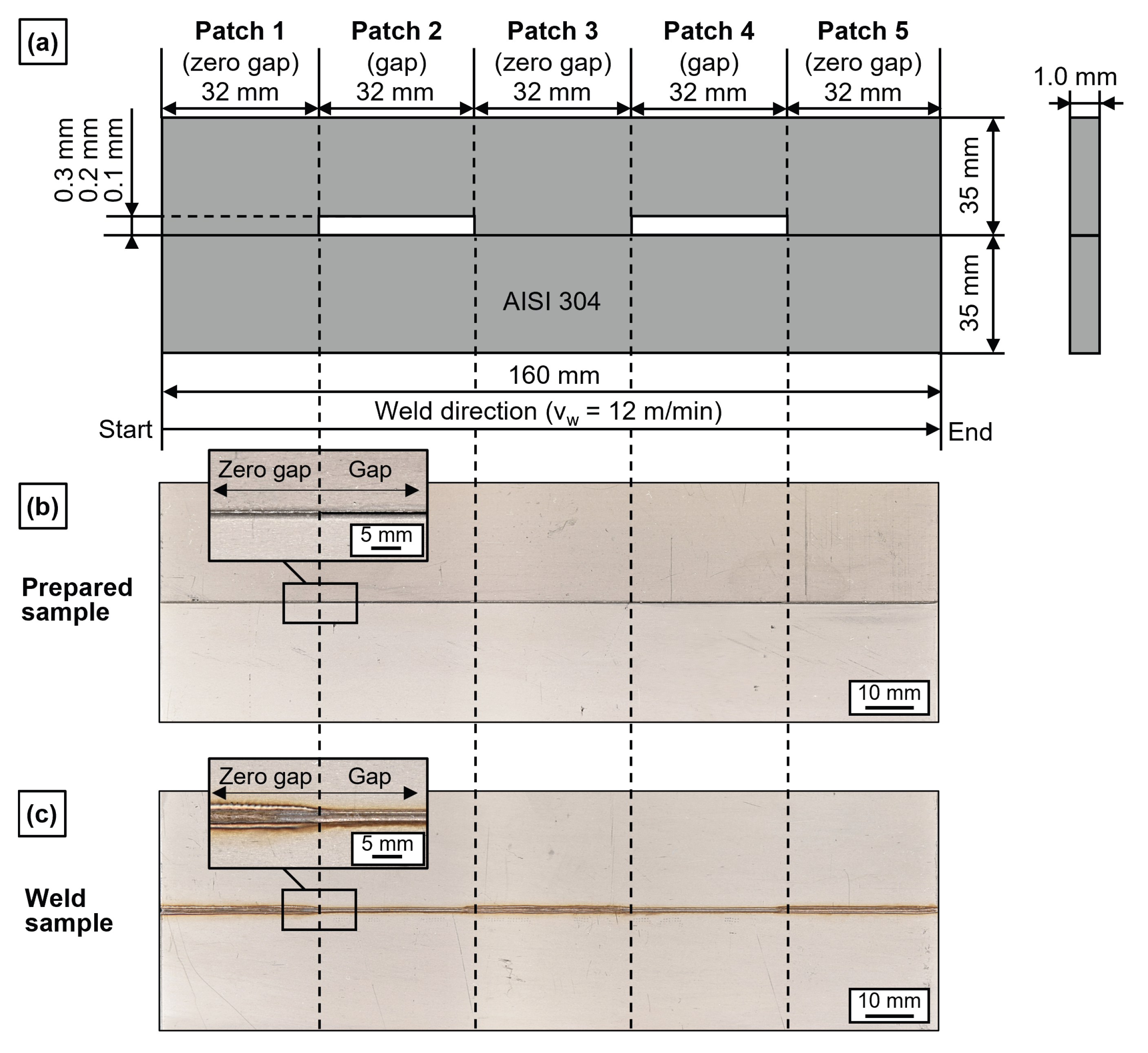
2.1. Specimen Configuration

The specimen configuration was selected as comparable to [14]. Two notches ($0.1$ $\mathrm{m}$$\mathrm{m}$, $0.2$ $\mathrm{m}$$\mathrm{m}$ and $0.3$ $\mathrm{m}$$\mathrm{m}$) were machined into one of the two butt-joined metal sheets of AISI 304 (X5CrNi18-10, 1.4301) high-alloy austenitic steel with a sheet thickness of 1 $\mathrm{m}$$\mathrm{m}$ to introduce defined gaps (cf. Figure 1). As a result, a total of 5 separate patch sections (3 × zero gap, 2 × joint gap) could be provided for each butt joint configuration. The tolerance of the gaps is approximately $0.06$ $\mathrm{m}$$\mathrm{m}$, which is the same as the overall production tolerances. The rolling direction of the sheets was identical to the welding direction.

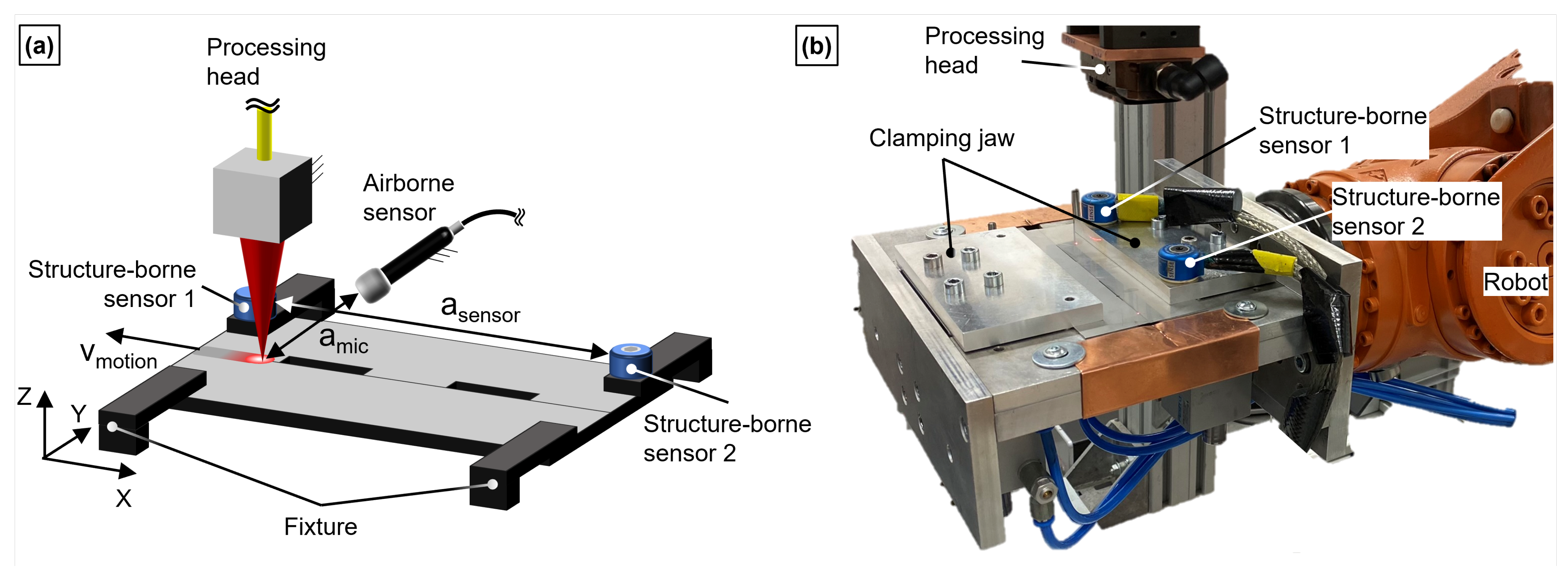
2.2. Weld and Measurement Setup

For the weld experiments, a disk laser (TruDisk 5000.75, Trumpf Laser und Systemtechnik GmbH, Ditzingen, Germany) with a maximum power of $P_{max}$ = 5 $\mathrm{k}$$\mathrm{W}$ and a wavelength of $\lambda =$ 1030 $\mathrm{n}$$\mathrm{m}$ was used. The laser source was coupled to a stationary arranged welding optic (BEO D70, Trumpf Laser und Systemtechnik GmbH, Ditzingen, Germany) as shown in Figure 2. A focus spot diameter of $d_{spot}=$ 600 $\mathsf{\mu }$$\mathrm{m}$ was selected for the experiments of this study. The specimens were fixed in a butt-joint configuration and handled by a six-axis robot (Kuka KR 60HA, Kuka AG, Augsburg, Germany). The weld parameters were set for full penetration, using a laser power of $P_L=$ $3.5$ $\mathrm{k}$$\mathrm{W}$ at a welding speed of $v_w$ = 12 $\mathrm{m}$/$\min$. For the acoustic emission (AE) signal acquisition, an in-house built airborne sound sensor (AB) was mounted on the stationary processing head. Furthermore, two structure-borne sound sensors were integrated into the specimen clamping, positioned at the beginning (SB1) and the end (SB2) of the notched sheet. Technical specifications of the sensors are given in

Table 1. Technical specifications of the used airborne and structure-borne-sound sensors.

Name	Type	Specifications	Distance
IZFP RI-MA71RC	Airborne	Center frequency: 520 $\mathrm{k}$$\mathrm{Hz}$
(AB)	ultrasound	Transducer diameter: 23 $\mathrm{m}$$\mathrm{m}$	$a_{mic}$ = 297 $\mathrm{m}$$\mathrm{m}$
	sensor	Focal point: 50 $\mathrm{m}$$\mathrm{m}$
QASS QWT sensors	Structure borne
(SB1: at the start,	ultrasound	Max frequency: 100 $\mathrm{M}$$\mathrm{Hz}$	$a_{sensor}$ = 114 $\mathrm{m}$$\mathrm{m}$
SB2: at the end)	sensor

. The airborne and structure-borne AE sensor data were captured using a data acquisition system (Optimizer 4D, QASS GmbH, Wetter, Germany) operating with a sampling rate of approximately 6250 $\mathrm{k}$$\mathrm{Hz}$ at a 16-bit resolution per channel. Upon measurements, several test experiments were conducted to determine the optimal operating point of the preamplifier of the data acquisition system. The cross jet was disabled during the experiments to provide an idealized data acquisition. Each gap configuration ($0.1$ $\mathrm{m}$$\mathrm{m}$, $0.2$ $\mathrm{m}$$\mathrm{m}$ and $0.3$ $\mathrm{m}$$\mathrm{m}$) was repeated 30 times to ensure a sufficient input for data processing.

3. Dataset and Cluster Analysis

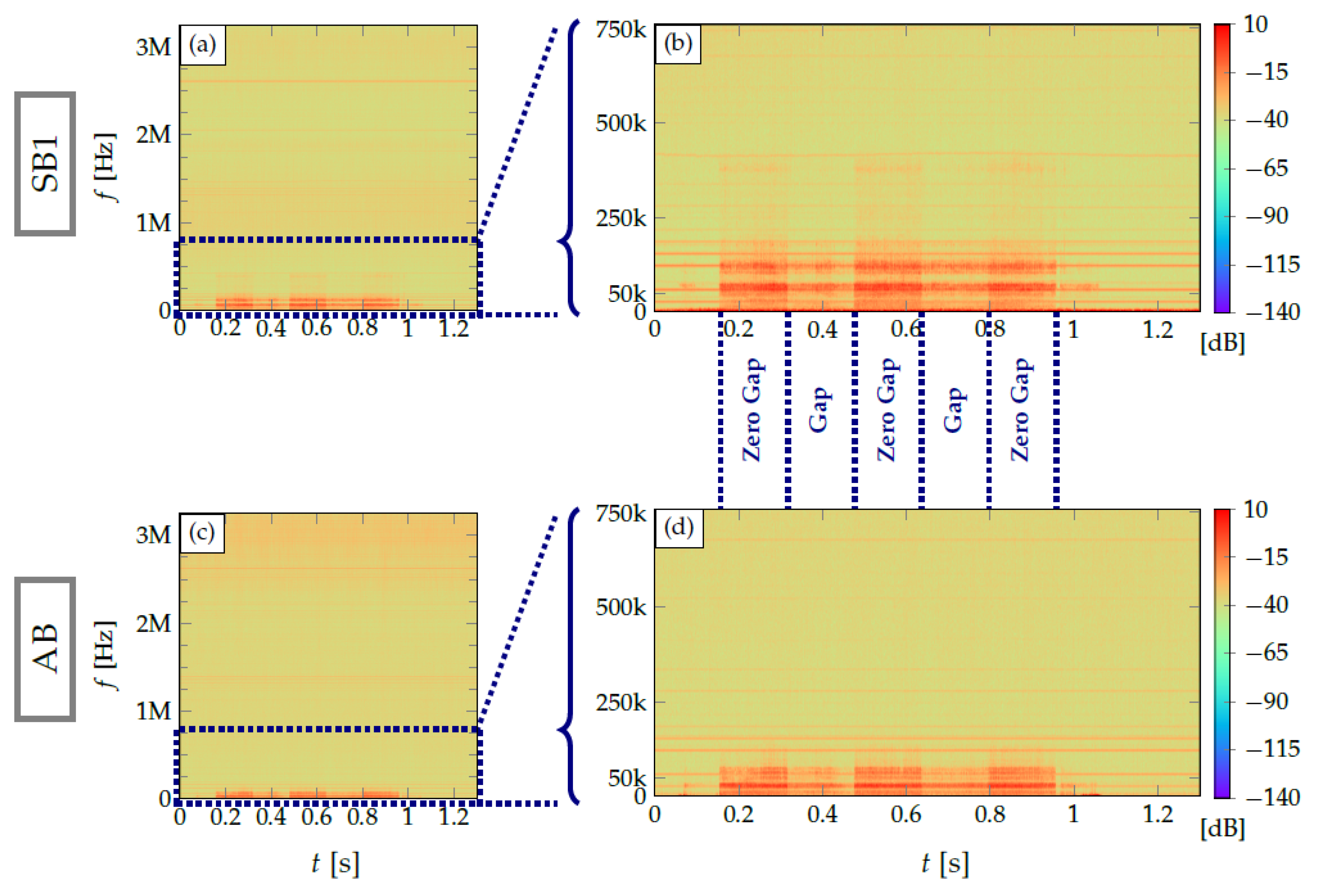
3.1. Signal Analysis

In this section, measurement data are briefly analyzed based on their spectrograms. A set of exemplary results are shown in Figure 3, where two metal sheets with two $0.3$ $\mathrm{m}$$\mathrm{m}$ gaps (Figure 1) are welded using a laser beam. For the purpose of visualization, two sensor signals are selected: the structure-borne sensor placed at the beginning of the specimen (SB1) and the airborne ultrasound sensor (AB). For computing the spectrograms, we used 2048 frequency bins with a window size of 2048, which is equivalent to $0.328$ $\mathrm{m}$$\mathrm{s}$. The window type used here is the Hanning window [23] with an overlap of 50%.

In general, the acoustic process emissions consist of four types of signals: signals correlated with properly welded joints in the Zero Gap sections, signals correlated with erroneous joints in the Gap sections, the acoustic emissions from the robotic arm movement and the environmental noise. In this work, the former two signals are denoted as weld-relevant signals, from which the information relevant to the welding process is attainable, and the latter two as the ambient noise. As mentioned in Section 2.2, acoustic emissions from a cross jet are not included in this study.

Our results in Figure 3a,b show that the weld-relevant signals are present below 400 $\mathrm{k}$$\mathrm{Hz}$ in the structure-borne sensor signal (SB1). In the airborne sensor signal (AB), the frequency range for the same information is reduced to below 125 $\mathrm{k}$$\mathrm{Hz}$ due to attenuation in the air (Figure 3c,d). Above those ranges, no weld-relevant signals can be visually perceived in the spectrograms for both sensor types. However, the relevant frequency range should be selected with care. To determine the frequency range, a significant reduction in the signal energy of interest needs to be identified. However, such reduction cannot be identified meaningfully without filtering out the ambient noise. It is even reported that some intrinsic changes in the signals are not easily perceptible for visual inspections [12]. Furthermore, weld-relevant signals were reported to be clearly observed in the frequencies above 1 $\mathrm{M}$$\mathrm{Hz}$, when the measurements were conducted using three different types of steels (DC04, DX51D, and S235JR+Z) with a focus spot diameter of 600 $\mathsf{\mu }$$\mathrm{m}$ and the laser power of 2 $\mathrm{k}$$\mathrm{W}$ at the welding speed of $1.2$ $\mathrm{m}$/$\min$ [16]. Unquestionably, the selection of specimen materials and/or the measurement configurations highly affect the frequency range. Yet, these suggest that there may be relevant information in higher frequencies of our measurement data, which is not visually observable in their spectrograms.

Nevertheless, visual inspection of the spectrograms can further confirm the correlation between the acoustic process emissions and the presence of a butt-joint gap or lack thereof. First, the signal energy is lowered within gap sections (Gap patches) for both sensor signals than within zero gap ones (Zero Gap patches). The distribution of the RMS values, which is equivalent to the signal energy, is provided for different gap sizes in [14]. The presence of a large-sized gap means less availability of the material to be welded, which consequently reduces laser-material interactions and, thus, its acoustic emissions. On top of that, the structure-borne sensor (SB1) reveals that the frequency range is also different between the Zero Gap and Gap patches. While the signal in the Zero Gap patches is observable up to 400 $\mathrm{k}$$\mathrm{Hz}$, the signal in the Gap patches is in a lower frequency range below 200 $\mathrm{k}$$\mathrm{Hz}$ and more frequency selective. Such change in the frequency range is, at least from the spectrograms, not observable in the airborne sensor signal (AB). It is also worth highlighting that the actual gap size in Zero Gap patches is not truly zero, and the largest gap was found to be $0.1892$ $\mathrm{m}$$\mathrm{m}$. The possible causes and the effects of such unintended gaps are discussed in [14], reporting increased difficulty in distinguishing $0.1$ $\mathrm{m}$$\mathrm{m}$ Gap signals from Zero Gap ones.

When it comes to ambient noise, multiple narrow-banded signals are prominently present in the entire frequency range. For a better understanding, only the ambient noise was recorded. Those recordings confirm that this narrow-banded interference was always observed when the robotic arm was moved. Since the environmental noise is innately wide-banded, it is highly likely that the robotic arm movement causes such narrow-banded acoustic emissions. Obviously, these multiple-band signals are harmonics of fundamental frequencies. However, the interval seems not to be constant, which makes it difficult to identify the fundamental frequencies. For instance, in Figure 3b two bands can be observed, one around 30 $\mathrm{k}$$\mathrm{Hz}$ and the other one around 60 $\mathrm{k}$$\mathrm{Hz}$, yet the third one is not around 90 $\mathrm{k}$$\mathrm{Hz}$ but instead around 120 $\mathrm{k}$$\mathrm{Hz}$. While the harmonics of 30 $\mathrm{k}$$\mathrm{Hz}$ are then barely observable between 250 $\mathrm{k}$$\mathrm{Hz}$ and 500 $\mathrm{k}$$\mathrm{Hz}$, the trace of such harmonics can be perceived again above 500 $\mathrm{k}$$\mathrm{Hz}$. Furthermore, some of the narrow-banded interference even fluctuates over the course of measurement, for instance, the band around 400 $\mathrm{k}$$\mathrm{Hz}$ in Figure 3b. These all suggest that canceling out such narrow-banded interference is not a trivial task. It requires either manual fine-tuning and selection of those bands, which needs to be repeated anew for different measurement setups, or an adaptive filtering technique.

3.2. Dataset Preparation

Based on the specimen configuration in Section 2.1, each recording file includes five 160 $\mathrm{m}$$\mathrm{s}$ patches as illustrated in Figure 3. This yields three Zero Gap and two Gap patches per file. Additionally, there are parts in each file that only capture the ambient noise, as the recording of the acoustic sensors extends beyond the period where the laser was actively welding. For the Gap class, a further classification is possible depending on the size as Gap 0.1 ($0.1$ $\mathrm{m}$$\mathrm{m}$ gap), Gap 0.2 ($0.2$ $\mathrm{m}$$\mathrm{m}$ gap) and Gap 0.3 ($0.3$ $\mathrm{m}$$\mathrm{m}$ gap). This enables the investigation of two different scenarios. Scenario I aims to investigate how the segment duration affects the accuracy of detecting a gap. This is achieved by classifying the segments into three classes, which are Zero Gap, Gap, and Noise. Scenario II, on the other hand, examines the relationship between the segment duration and the accuracy of identifying the gap size, coping with the more detailed information about the severity of weld failures. Here, the signal segments are classified into five classes, which are Zero Gap, Gap 0.1, Gap 0.2, Gap 0.3, and Noise.

The segments of Noise class are selected from the signal part after $1.2$ $\mathrm{s}$, including the environmental noise as well as the interference from the robotic arm movement discussed in Section 3.1. Noise segments are included for the following reasons. Noise and interference from the environment are always present and appear as multiple narrowband signals in the same frequency range as that of the acoustic emissions from welding, as discussed in Figure 3. Although filtering out such interference is beyond the scope of this study, their impact on the informativeness of signal segments, especially when dealing with a very short segment, is of great interest. For instance, if a Gap 0.1 segment is misclassified as a Zero Gap segment, this still ensures that the segment contains at least some information about the welding process. However, if the same segment is misclassified as Noise, this implies that the weld-relevant information can no longer be extracted.

To align with the purpose of this study, some files and parts of the recording need to be excluded, such that each signal segment corresponds to a single class regardless of its duration. As discussed in Section 3.1, the presence of unintended large gaps in Zero Gap patches makes the distinction between Zero Gap and small-sized Gap patches ambiguous [14]. For this reason, the recording files containing any Zero Gap patches larger than $0.07$ $\mathrm{m}$$\mathrm{m}$ were excluded from the dataset. A summary of the file count for each gap size is provided in

Table 2. Summary of file counts.

File Type	File Count
Gap 0.1 + Zero Gap + Noise	15
Gap 0.2 + Zero Gap + Noise	22
Gap 0.3 + Zero Gap + Noise	23

. It is important to note that this study sticks to the labels based on the original specimen configurations. However, relabeling of the data is possible, which is discussed in [14]. Another measure was to remove the transitions between two consecutive patches from the dataset. This is due to its extremely short and unknown duration, prohibiting it from forming its own class with a sufficient number of samples. To ensure that no signal segments include any transition phase, the transitions were eliminated from each recording by trimming the beginning and end of each patch by 20 $\mathrm{m}$$\mathrm{s}$.

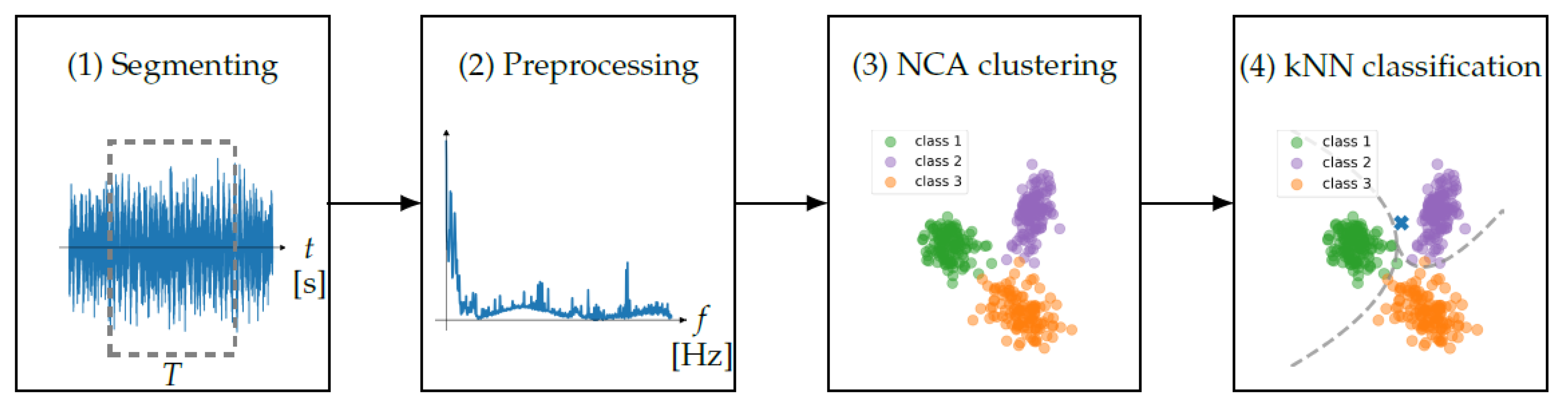
3.3. Clustering Technique

A crucial step of cluster analysis is selecting a similarity metric. A similarity metric determines how the available data are evaluated and placed accordingly in a given coordinate and/or scored for clustering. Clearly, the performance of clustering highly depends on the quality of the metric. Since general-purpose metrics such as the Euclidean distance often fail to capture the intrinsic yet possibly not obvious features of the data of interest, an appropriate metric needs to be selected with care [24]. For selecting a similarity metric, which is closely related to distance metric learning, the task at hand needs to be taken into account. Considering the interests of this study, the k-nearest neighbors (kNN) algorithm [25] is selected as a classifier since it is non-parametric and does not require any training, making its results directly reflect the cluster performance. Among the distance metric learning methods specifically targeted for kNN classification, Neighborhood Components Analysis (NCA) [26] is selected for this study as it allows the reduction of the data dimension [24]. Dimension reduction is useful for our research, where the input data size is much larger compared to the number of classes and possibly the size of the relevant feature domain. In essence, NCA is a supervised Mahalonobis distance learning, which linearly transforms the input data $\mathbf{x}$ $\in {\mathbb{R}}^N$ into a suitable domain with the output $\mathbf{y}$ $\in {\mathbb{R}}^M$. NCA is also a non-parametric method and thus does not make any assumption on data statistics or shapes, which is also favorable for this study.

4. Results and Discussions

In this section, the informativeness of acoustic process emissions is evaluated and compared for various durations. As previously discussed, the informativeness of signal segments is represented by the performance of NCA cluster analysis, specifically the separability of different classes. The class separability is assessed based on the classification accuracy of resulting clusters, which enables numerical comparison. Since NCA requires training to learn the optimal distance metric, the available dataset needs to be split into the training and test sets. To mitigate the effect of such randomness on the results, this study conducted repeated learning-testing (RLT) validation [27], which is also known as Monte Carlo cross-validation. This method repeats the learning-testing process where the dataset is randomly split anew for each iteration.

4.1. Validation Setup and Parameters

For each segment duration, 50 learning-testing iterations were conducted, each of which consists of the following four steps (Figure 4). First, the signals are segmented with the given duration T in the time domain. After segmentation, a fixed number of segments are randomly selected from the measurement data for training and testing. To make the training fair, the number of segments is kept constant for both the training and the test set, regardless of the segment duration. Without this measure, very short-duration segments yield a much larger sample size in the training set than long-duration segments, resulting in easier training and, thus, higher accuracy. Second, the selected segments are preprocessed to enhance the signal structure and format them into the same data size regardless of their duration. This is achieved by computing short-time Fourier transform (STFT) and averaging them over time. The averaged power spectral density is then standardized such that each has a zero mean and unit variance. Third, NCA is trained using the training segments to learn the optimal metric. This step is equivalent to supervised clustering. Lastly, the test segments, which are not used for training, are linearly transformed by the trained NCA and then classified using kNN.

A summary of the validation parameters is given in

Table 3. Validation parameter values

Operation	Parameter	Value
RLT validation	Number of iterations	50
	Segment durations	1… 100 $\mathrm{m}$$\mathrm{s}$
	Scenario I	120 segments per class
	Scenario II	30 segments per class
	Data split ratio	67% training
		33% test
STFT	Sampling frequency	6$\mathrm{M}$$\mathrm{Hz}$
	Frequency bins	2048
	Time window	2048 samples (≈ $0.341$ $\mathrm{m}$$\mathrm{s}$)
	Window type	Hanning window
	Overlap	50%
NCA	Initialization	linear discriminant analysis
	Input size	2048
	Output size	$N_{class}-1$
kNN	k	3

. For the investigation, the range between 1 $\mathrm{m}$$\mathrm{s}$ and 100 $\mathrm{m}$$\mathrm{s}$ was selected for segmenting the recording of each patch. As discussed in Section 3.2, both ends of each patch were trimmed by 20 $\mathrm{m}$$\mathrm{s}$ to eliminate the transitions, yielding 120 $\mathrm{m}$$\mathrm{s}$ long recording for each patch. However, it is unclear how long the effect of the transitions lasts, and a longer segment such as 120 $\mathrm{m}$$\mathrm{s}$ one may be affected by the transitions from both ends. In such cases, the performance comparison among different durations becomes unfair. To mitigate the effect of transitions as much as possible, an upper bound of 100 $\mathrm{m}$$\mathrm{s}$ was introduced. Furthermore, no other processing techniques were applied to the signals aside from resampling them with the sampling frequency of 6 $\mathrm{M}$$\mathrm{Hz}$ prior to segmentation. To incorporate the possibly imperceptible information hidden in the high-frequency range, the entire frequency range of 3 $\mathrm{M}$$\mathrm{Hz}$ was used. For NCA clustering and kNN classification, the Python library scikit-learn [28] was used. The clustering and classification parameters were empirically selected by comparing the performance obtained using various values.

Strictly speaking, it is not fair to compare the performance among different sensor signals listed in Table 1, as these sensors have different sensitivity and characteristics. Nevertheless, comparing the performance among different sensor types can illuminate the advantages and drawbacks of different sensing methods. To highlight the informativeness of each sensor, the investigation of this study treats each sensor individually instead of fusing them. Possible benefits of sensor fusion are discussed based on the obtained results in Section 5. Note that the results of the structure-borne sensor placed at the end of the specimen (SB2) are omitted from the discussion in the subsequent sections. This is because they are found to be very similar to those of the other structure-borne sensor placed at the beginning of the specimen (SB1). Although sensor location does not have a significant effect on the informativeness of the signals of our study, a larger deviation will likely be observed in the results if the sensors are placed farther apart.

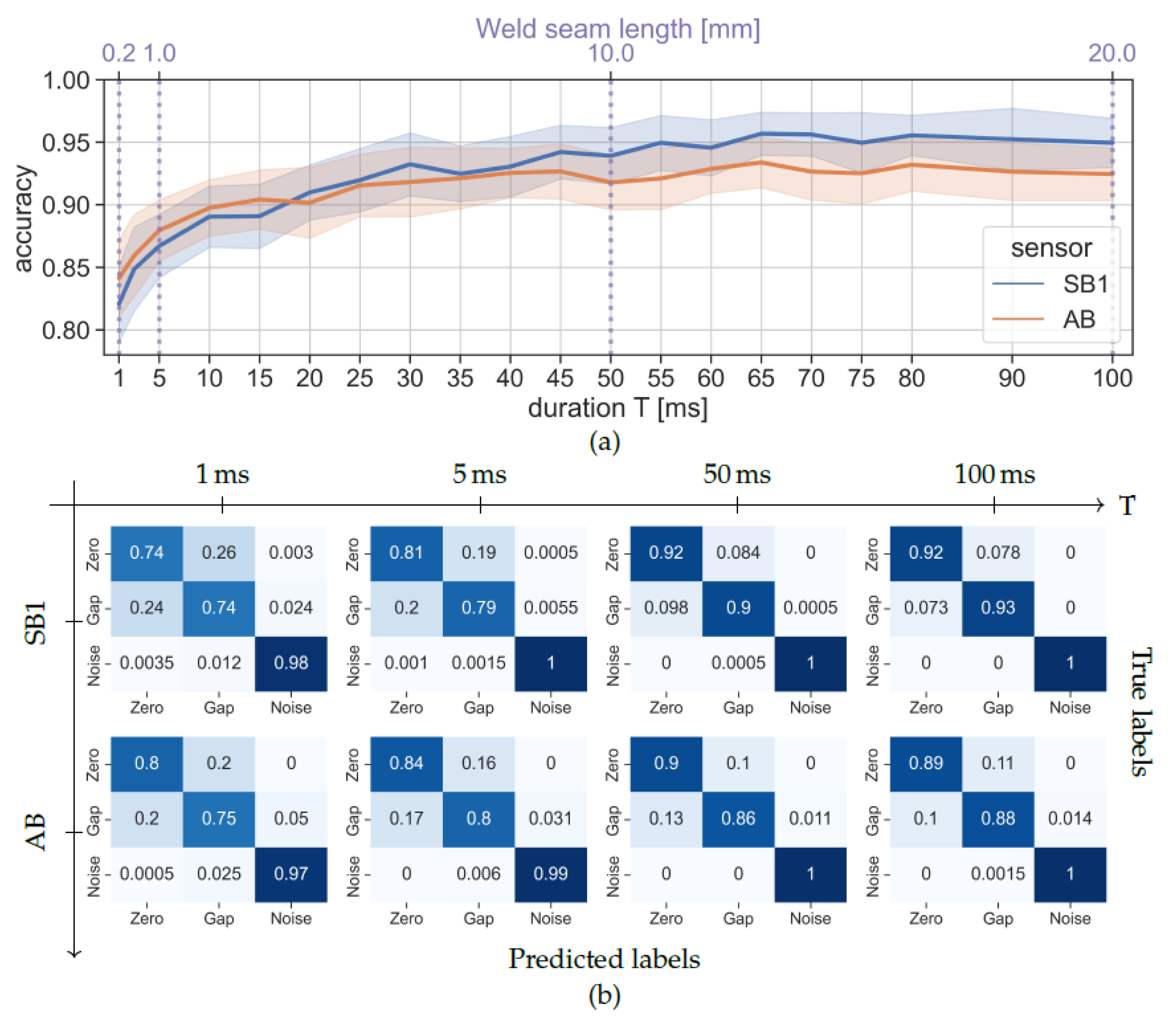
4.2. Scenario I: Gap Detection

The investigation results of gap detection are presented in Figure 5 and Figure 6. Figure 5a shows the average accuracy over varying segment durations, while the average confusion matrices are shown for a selected set of durations in Figure 5b. In Figure 6, a set of clustering results are presented as examples.

Figure 5a demonstrates that overall the accuracy of both sensor types steadily increases with duration until it starts to converge from a certain saturation point. This suggests that the segments longer than such saturation point can be shortened without loss of weld-relevant information. The saturation point, however, varies depending on the sensor type. Specifically, the saturation points of the structure-borne sensor signals (SB1) and the airborne sensor signals (AB) are around 50$\mathrm{m}$$\mathrm{s}$ and 25 $\mathrm{m}$$\mathrm{s}$, respectively. This difference in their saturation behavior accounts for their performance difference. If segments are longer than 40 $\mathrm{m}$$\mathrm{s}$, structure-borne sensor signals (SB1) slightly outperform the airborne sensor signals (AB), resulting in the maximum accuracy of 95% for the structure-borne sensor and 92.5% for the airborne sensor. This can be attributed to the information loss in higher frequencies due to attenuation in air, as shown in Figure 3. For the segments shorter than 40 $\mathrm{m}$$\mathrm{s}$, however, there seems to be no significant difference in performance among different sensors. If a segment is shorter than 5 $\mathrm{m}$$\mathrm{s}$, the accuracy of both sensors drops sharply, indicating the difficulty in extracting the weld-relevant information.

A similar behavior can be observed in the confusion matrices, too (Figure 5b). Comparing the results of 100 $\mathrm{m}$$\mathrm{s}$ and 50 $\mathrm{m}$$\mathrm{s}$, the difference seems to be marginal for both structure-borne sensor signals (SB1) and airborne sensor signals (AB). This again suggests that 50 $\mathrm{m}$$\mathrm{s}$ suffices to extract the same amount of the information contained in a 100 $\mathrm{m}$$\mathrm{s}$ segment, which enables almost 90% accuracy to distinguish Zero Gap and Gap joints. If the segments are shorter than 5 $\mathrm{m}$$\mathrm{s}$, misclassification of noise segments starts to increase, also signifying that extracting the relevant information becomes more challenging.

Figure 6 provides more insights into the segment separability. As an example, a set of NCA clustering results are shown for 100 $\mathrm{m}$$\mathrm{s}$, 50 $\mathrm{m}$$\mathrm{s}$, 5 $\mathrm{m}$$\mathrm{s}$ and 1 $\mathrm{m}$$\mathrm{s}$ segments. Here, clustering was computed using the test set, which is not used for training. In general, the distance between clusters increases with segment duration. This suggests that longer segments contain sufficient weld-relevant information, which allows NCA to learn an appropriate transformation of the segments.

Comparing the separability of 100 $\mathrm{m}$$\mathrm{s}$ and 50 $\mathrm{m}$$\mathrm{s}$ segments in Figure 6, the separation of clusters is strikingly similar, which also indicates that the same amount of the information is preserved even if signal segments are halved from 100 $\mathrm{m}$$\mathrm{s}$ to 50 $\mathrm{m}$$\mathrm{s}$. Another finding is that the clusters of the airborne sensor segments (AB) are located closer to each other than those of the structure-borne sensor segments (SB1). These results also imply that there seems to be more weld-relevant information available in the structure-borne signals when it comes to detecting joint gaps.

A noticeable change can be observed in the cluster separability for both sensor signals when the results of 50 $\mathrm{m}$$\mathrm{s}$ segments are compared to those of 5 $\mathrm{m}$$\mathrm{s}$. With 5 $\mathrm{m}$$\mathrm{s}$ segments, the Zero Gap cluster is closer to the Gap cluster, causing a larger overlap of these two classes. Indeed, the average accuracy of distinguishing Zero Gap and Gap segments is significantly reduced, as shown in Figure 5b. This may be attributed to the fact that the actual gap size of Zero Gap patches is not zero, making the distinction of smaller gaps from Zero Gap difficult. This trend continues when segments become further shorter to 1 $\mathrm{m}$$\mathrm{s}$, which is equivalent to $0.2$ $\mathrm{m}$$\mathrm{m}$ weld seam, where the clusters of all classes are closer and the separation of one another is ambiguous. It is also worth noticing that the size of the Zero Gap and the Gap clusters resembles that of the noise cluster for shorter segments, implying that the effect of noise becomes larger with decreasing duration.

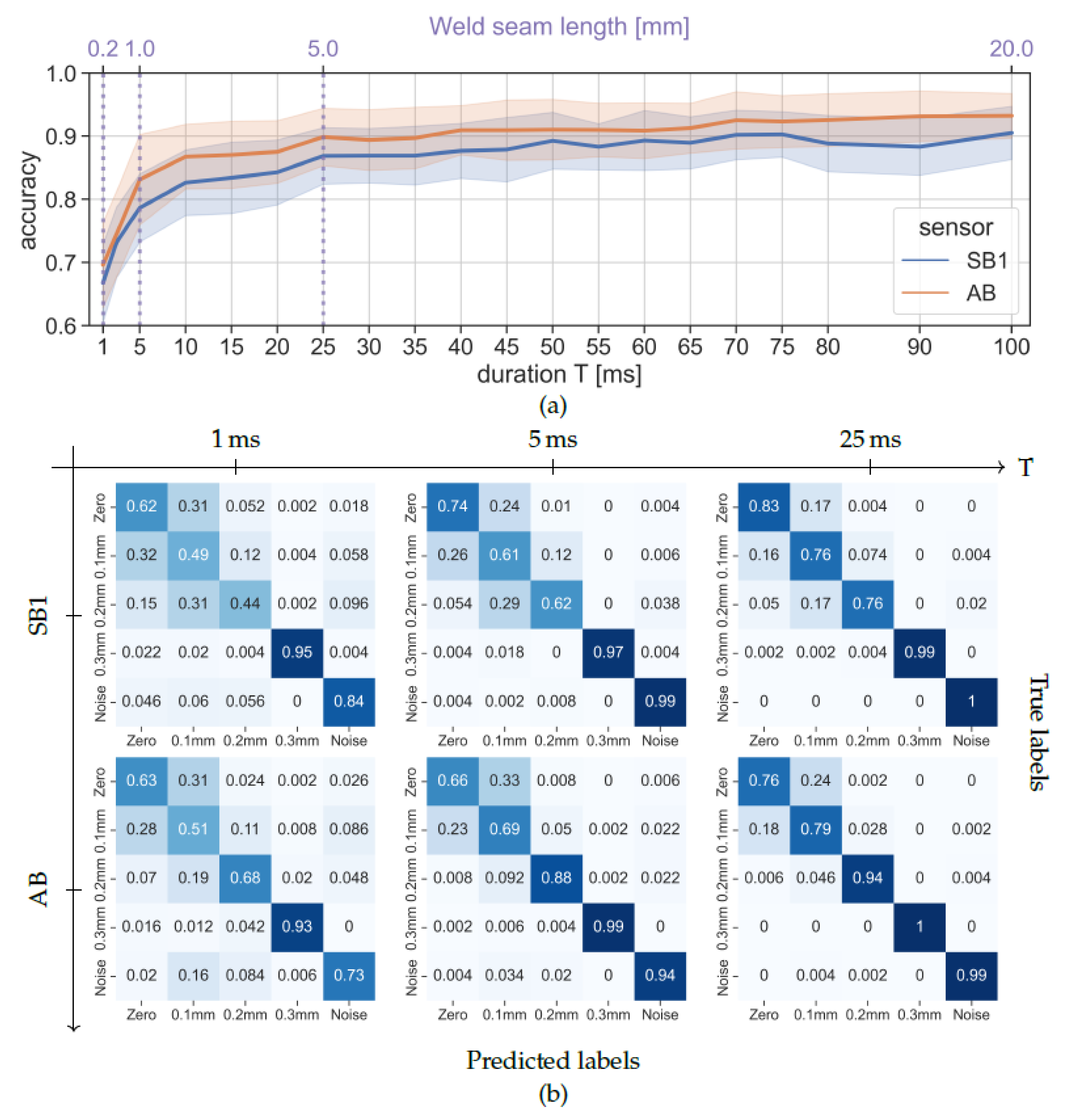
4.3. Scenario II: Identification of Gap Size

This section provides the investigation results of Scenario II, where gap size is identified from acoustic process emissions. This scenario aims to illustrate whether the information in a segment suffices to determine the severity of error in a joint, dealing with more detailed information than Scenario I. Since it involves more classes than Scenario I, visualizing the class separability is not possible. Consequently, the informativeness of signal segments is assessed using both classification accuracy and relative recall presented in Section 4.3.1 and Section 4.3.2, respectively.

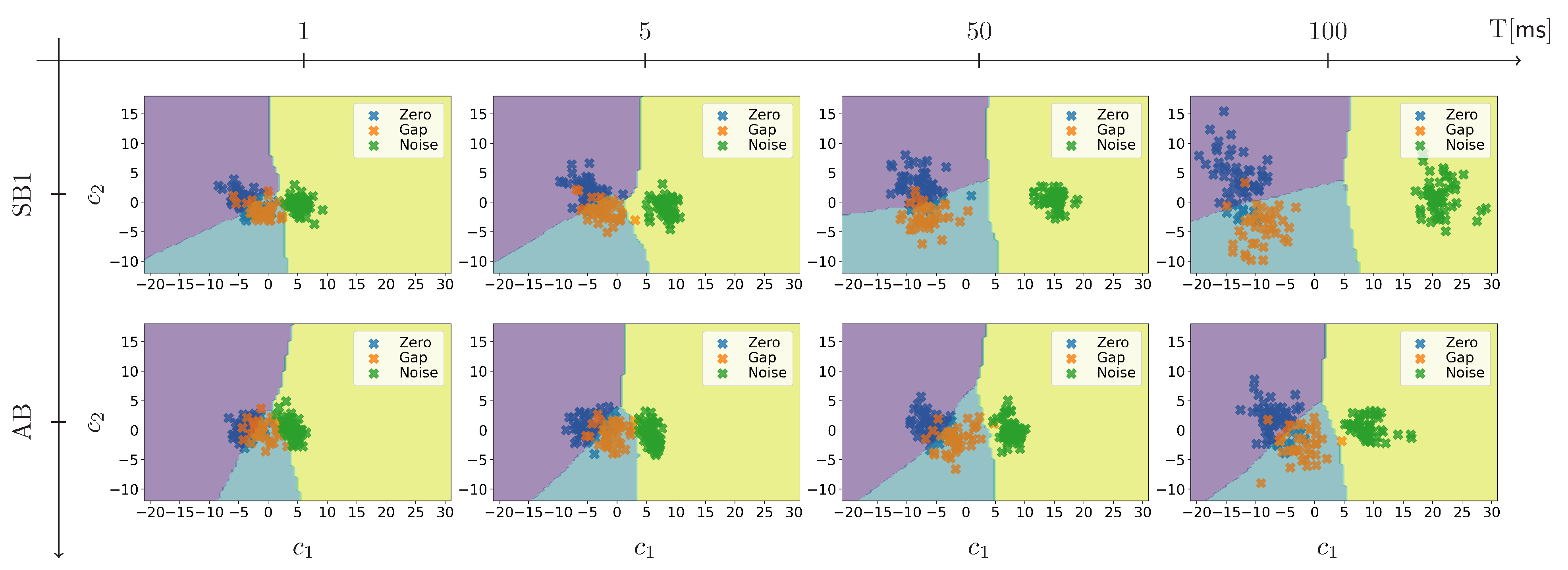
4.3.1. Classification Accuracy

Figure 7a shows the average accuracy of 50 RLT iterations over varying segment durations. Overall, the accuracy of quantifying the gap size is lower compared to that of gap detection. This is particularly true for the structure-borne sensor (SB1), whose highest accuracy is around 90%. On the other hand, the highest accuracy of the airborne sensor (AB) is slightly below 92.5%. Nevertheless, in a similar manner to that observed with gap detection, the accuracy of identifying gap size increases with duration and starts to saturate from a certain point. Contrary to gap detection, both sensors have similar saturation points at around 25 $\mathrm{m}$$\mathrm{s}$ when it comes to identifying the gap size. This indicates that signal segments can be shortened to 25 $\mathrm{m}$$\mathrm{s}$ while maintaining their informativeness about the gap size. Noticeably, the accuracy of airborne sensor signals (AB) is consistently higher than that of structure-borne sensor signals (SB1). The possible reasons for this performance difference will be discussed in this section.

For further insights, the average confusion matrices are provided in Figure 7b for three different durations. Compared to other classes, classification accuracy for identifying a $0.3$ $\mathrm{m}$$\mathrm{m}$ gap (Gap 0.3) remains remarkably high under varying durations for both sensor types. This implies that an adequate-sized gap results in signal characteristics that are observable in a very short duration of acoustic process emissions. Interestingly, if segment duration is 1 $\mathrm{m}$$\mathrm{s}$, the Gap 0.3 segments can be better predicted than the Noise segments, where the Noise segments are misclassified more as Zero Gap segments than Gap 0.3 ones. This suggests that the acoustic emissions induced by a large-sized gap are not merely the lack of emissions and a decrease in signal energy but also have distinctive signal characteristics.

When the results of both sensor types are compared, the accuracy of classifying Gap 0.2 is significantly different. If segments are longer than 25 $\mathrm{m}$$\mathrm{s}$, airborne sensor signals (AB) yield 94% accuracy of correctly classifying the Gap 0.2 segments, whereas the accuracy of structure-borne signals (SB1) is low around 75%. This tendency continues when segments become shorter. A possible explanation for the impaired accuracy is the difficulty in maintaining the same measurement condition for the structure-borne sensors. The structure-borne sensors were mounted anew every time a new specimen was set. Since each file corresponds to a different specimen, the variance among files may be larger for the structure-borne sensor signals. Moreover, during the measurement of Gap 0.2 specimens, the sensors needed to be recalibrated, which may have led to a change in signal characteristics before and after the calibration. Both suggest that a stable mounting technique should be established for structure-borne sensors to ensure consistent and reliable inspection quality.

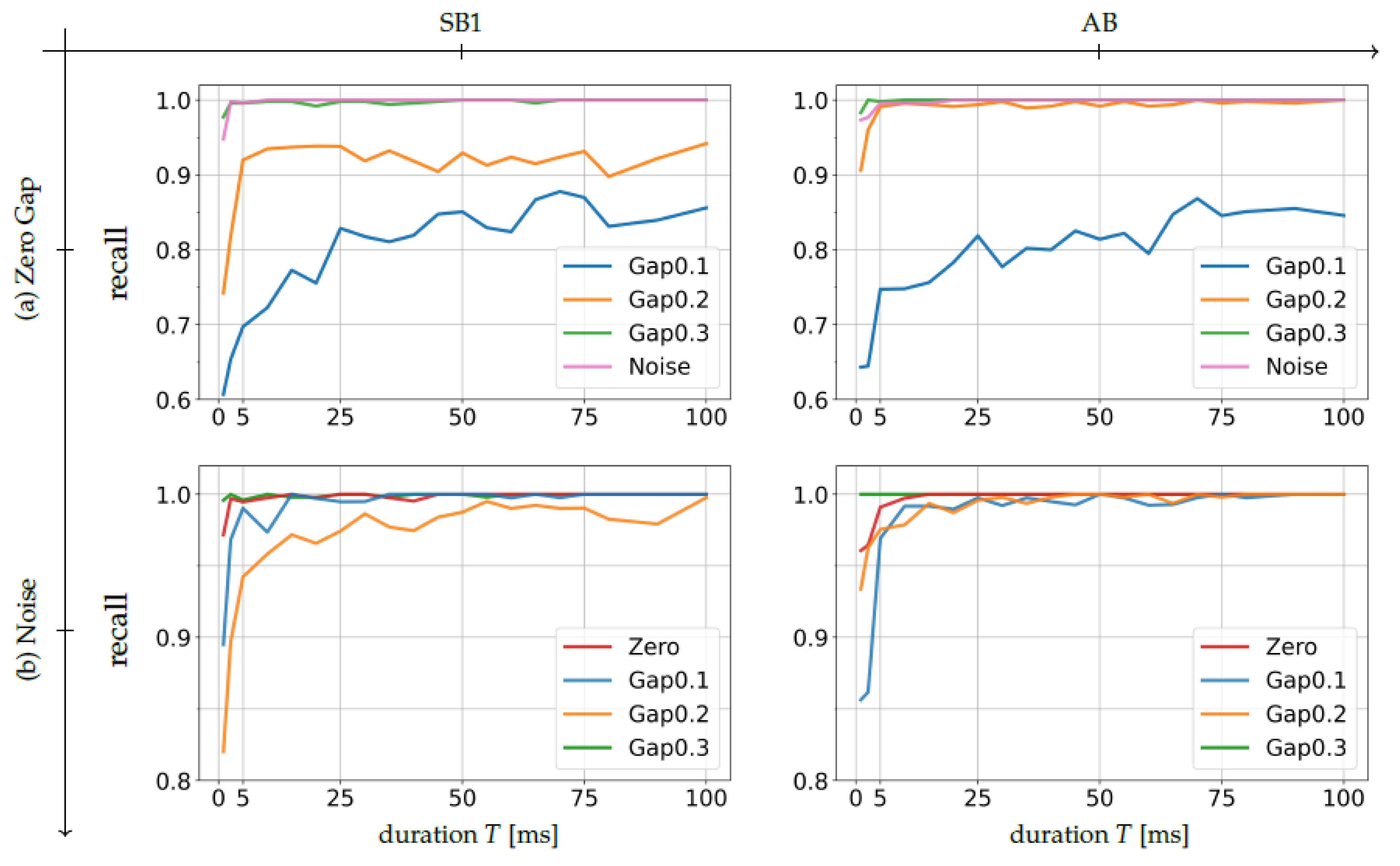
4.3.2. Separability Analysis Using Relative Recall

Contrary to Scenario I, visualizing the separability of five classes is not trivial as the clustering outputs consist of four features, requiring 4D plots. However, considering only two classes at a time enables to handle the classification results as that of binary classification. One metric to evaluate binary classification is recall, also known as the true positive rate. The recall is essentially a ratio of the true positive to all positive predictions. As an example, consider the confusion matrix of the structure-borne sensor (SB1) for 25 $\mathrm{m}$$\mathrm{s}$ shown in Figure 7b. Its relative recall of the Gap 0.1 class with respect to Zero Gap one can be computed as $\frac{0.76}{(0.76+0.16)}=0.826$. The reason for using recall to evaluate the class separability is that the relative recall represents the misclassification rate. If, for instance, Gap 0.1 segments tend to be misclassified as Zero Gap one, then the Gap 0.1 cluster is likely to be very close to the Zero Gap cluster than other clusters whose misclassification rate is low. This means that a high relative recall indicates good separability of the reference class from another one and vice versa.

The relative recall results over varying durations are presented in Figure 8. Figure 8a shows the relative recall with respect to the Zero Gap class, aiming to demonstrate how separable the Zero Gap cluster is from the other classes. Using the same analogy, Figure 8b presents the relative recall with respect to the Noise class.

Focusing on the results shown in Figure 8a, two things are common for both sensor types. First, the Gap 0.1 segments seem to be very difficult to distinguish from the Zero Gap ones. Here, even 100 $\mathrm{m}$$\mathrm{s}$ segments can achieve only around 85% recall, demonstrating that making a segment longer does not necessarily increase the sensitivity with regard to the gap size. This can be attributed to two factors. On the one hand, the actual gap size of Zero Gap patches is not exactly zero, as discussed in Section 3.1, making the distinction between these two classes ambiguous. On the other hand, the laser spot diameter ($0.6$ $\mathrm{m}$$\mathrm{m}$) is large relative to the gap size of $0.1$ $\mathrm{m}$$\mathrm{m}$. Such a relatively large laser beam can ignore a small-sized gap and may produce acoustic process emissions very similar to the one that is produced with Zero Gap joints. Another finding is that the relative recall of the Gap 0.3 class is and remains very high up to 1 $\mathrm{m}$$\mathrm{s}$. This suggests high separability of the Zero Gap and the Gap 0.3 clusters. This is also true for the Noise class, yet its recall reduces slightly more than that of the Gap 0.3 class if the segments are shorter than 5 $\mathrm{m}$$\mathrm{s}$.

A striking difference among different sensor types can be observed with the relative recall of the Gap 0.2 class. In the same way as the confusion matrices, the structure-borne sensor signal (SB1) exhibits a much lower recall regardless of the segment duration. This is suspected to result from the aforementioned inconsistency in the signals. In contrast, the airborne sensor signals (AB) yield a very high recall of the Gap 0.2 class, indicating that the Zero Gap class is also well separable from the Gap 0.2 class. Comparing the airborne sensor results (AB) of the Gap 0.2 and the Gap 0.3 class, the Zero Gap cluster seems slightly closer to the Gap 0.2 cluster than to the Gap 0.3 one.

The same behavior can be seen in the relative recall of the Gap 0.2 class with respect to the Noise class in Figure 8b. Here again the structure-borne sensor signals (SB1) yield a much lower recall of the Gap 0.2 class than other classes, exhibiting the difficulty in correctly classifying the Gap 0.2 segments. Considering its relative recall to the Zero Gap as well, it is highly likely that the Gap 0.2 data have a larger variance than other classes. For the rest of the classes, the relative recall with respect to the Noise class is very high (>97.5%) up to 10 $\mathrm{m}$$\mathrm{s}$. This demonstrates that the Noise cluster is well separable, and therefore, the weld-relevant information is sufficiently available in segments longer than 10 $\mathrm{m}$$\mathrm{s}$. It is worth noticing that the Gap 0.3 class achieves almost 100% recall even with 1 $\mathrm{m}$$\mathrm{s}$ segments, equivalent to $0.2$ $\mathrm{m}$$\mathrm{m}$ of the weld seam. This is another indicator that the acoustic emissions induced by a large-sized gap are not merely the absence of emission but also exhibit unique signal characteristics.

Lastly, a few remarks on the effect of noise should be added. Both results in Figure 8 reveal that the separability of different classes becomes more challenging if segments are shorter than 5 $\mathrm{m}$$\mathrm{s}$, which is equivalent to 1 $\mathrm{m}$$\mathrm{m}$ weld seam. Because such short segments tend to be misclassified as the Noise class, these results imply that the effect of noise becomes more crucial when segments become shorter.

5. Conclusions

In this study, the temporal resolution of acoustic process emissions is addressed toward realizing real-time acoustic process monitoring and controlling systems for laser welding. Considering that the resolution varies depending on the specific information being sought, this study aims to investigate the relationship between the signal duration and their informativeness to identify and quantify joint gaps in laser butt welding. For this purpose, cluster analysis of signal segments was conducted, whose classification accuracy was used for evaluating the segment informativeness.

The obtained results reveal that the signal segments can be shortened to a certain point while preserving their informativeness. Such a point, however, varies depending on the sensor type and the task at hand. With our specific configuration using the laser power of $3.5$ $\mathrm{k}$$\mathrm{W}$ at a welding speed of 12 $\mathrm{m}$/$\min$, structure-borne sensor signals can be shortened to 50 $\mathrm{m}$$\mathrm{s}$, yielding almost 95% gap detection accuracy. For the same task of gap detection, airborne sensor signals can be shortened further to 25 $\mathrm{m}$$\mathrm{s}$, maintaining 92.5% accuracy. When it comes to identifying the gap size, 25 $\mathrm{m}$$\mathrm{s}$ suffices to maximize the segment informativeness regardless of sensor type. However, the highest achievable accuracy is lower than that of gap detection. These findings encourage the optimization of the segment duration in accordance with the task and the required accuracy.

Furthermore, the airborne sensor in our study demonstrates more reliable detection and classification accuracy compared to its structure-borne counterparts. This results from a large variability in structure-borne sensor signals due to their susceptibility to renewal mounting. For maintaining signal quality, a reliable mounting technique needs to be established. Another remarkable finding is that large-sized gaps, specifically $0.3$ $\mathrm{m}$$\mathrm{m}$ asymmetric gaps, demonstrate the induction of unique characteristics in the acoustic process emissions, which is not a mere decrease in signal energy. This poses the question of what such unique characteristics look like and how they differ from those induced by small-sized gaps.

The following are the possible research topics for enabling real-time acoustic monitoring systems based on the findings of this study. The obtained results demonstrate that the effect of noise increases when signal segments become shorter. This indicates that alleviating the effects of noise is beneficial for real-time applications. Sensor data fusion can also improve the temporal resolution because the kind and the availability of weld-relevant information seem to vary depending on the sensor type. To optimally place the sensors, the emission directivity needs to be identified. Considering the actual monitoring setups, the monitoring system also needs to cope with the transitions between a zero gap patch and a gap one, requiring further investigation. Because different welding configurations, such as welding speed or different materials, effect the signal characteristics of the acoustic emissions, such effects need to be studied as well. Another important aspect of the practice is compatibility with a crossjet, which produces substantial acoustic emissions in the same frequency range as that of the weld-relevant signals [13]. For realizing in-process monitoring systems, a measure to mitigate its effect is indispensable.

Lastly, it is also worth paying attention to sensor integration. For achieving low latency, recordings need to be synchronized with the welding process. This requires identifying the exact time point when the welding process is started. For this purpose, this study employed a synchronization device, which was triggered by a high-speed camera serving as a reference. To ease the installation effort in practice, however, a synchronization measure based solely on acoustic sensors is beneficial. Because the acoustic emission of the ambient noise is shown to be easily distinguishable from that of weld-relevant signals, acoustic sensor signals have the potential to be utilized for synchronization purposes as well.

References

1. Katayama, S.; Tsukamoto, S.; Fabbro, R. Handbook of Laser Welding Technologies; Woodhead Publishing Series; Woodhead Publishing: Cambridge, UK, 2013. [Google Scholar]
2. Fabbro, R. Melt pool and keyhole behaviour analysis for deep penetration laser welding. J. Phys. D Appl. Phys. 2010, 43, 445501. [Google Scholar] [CrossRef]
3. Fabbro, R.; Slimani, S.; Coste, F.; Briand, F. Analysis of the various melt pool hydrodynamic regimes observed during cw Nd-YAG deep penetration laser welding. In International Congress on Applications of Lasers & Electro-Optics; Laser Institute of America: Orlando, FL, USA, 2007; Volume 2007. [Google Scholar] [CrossRef]
4. Sudnik, W.; Radaj, D.; Erofeew, W. Computerized simulation of laser beam weld formation comprising joint gaps. J. Phys. D Appl. Phys. 1998, 31, 3475. [Google Scholar] [CrossRef]
5. Seang, C.; David, A.; Ragneau, E. Nd:YAG Laser Welding of Sheet Metal Assembly: Transformation Induced Volume Strain Affect on Elastoplastic Model. Phys. Procedia 2013, 41, 448–459. [Google Scholar] [CrossRef]
6. Hsu, R.; Engler, A.; Heinemann, S. The gap bridging capability in laser tailored blank welding. In International Congress on Applications of Lasers & Electro-Optics; Laser Institute of America: Orlando, FL, USA, 1998; pp. F224–F231. [Google Scholar]
7. Walther, D.; Schmidt, L.; Schricker, K.; Junger, C.; Bergmann, J.P.; Notni, G.; Mäder, P. Automatic detection and prediction of discontinuities in laser beam butt welding utilizing deep learning. J. Adv. Join. Process. 2022, 6, 100119. [Google Scholar] [CrossRef]
8. Schricker, K.; Schmidt, L.; Friedmann, H.; Bergmann, J.P. Gap and Force Adjustment during Laser Beam Welding by Means of a Closed-Loop Control Utilizing Fixture-Integrated Sensors and Actuators. Appl. Sci. 2023, 13, 2744. [Google Scholar] [CrossRef]
9. Huang, W.; Kovacevic, R. Feasibility study of using acoustic signals for online monitoring of the depth of weld in the laser welding of high-strength steels. Proc. Inst. Mech. Eng. Part B J. Eng. Manuf. 2009, 223, 343–361. [Google Scholar] [CrossRef]
10. Authier, N.; Touzet, E.; Lücking, F.; Sommerhuber, R.; Bruyère, V.; Namy, P. Coupled membrane free optical microphone and optical coherence tomography keyhole measurements to setup welding laser parameters. In High-Power Laser Materials Processing: Applications, Diagnostics, and Systems IX; Kaierle, S., Heinemann, S.W., Eds.; International Society for Optics and Photonics, SPIE: Bellingham, WA, USA, 2020; Volume 11273, p. 1127308. [Google Scholar] [CrossRef]
11. Li, L. A comparative study of ultrasound emission characteristics in laser processing. Appl. Surf. Sci. 2002, 186, 604–610. [Google Scholar] [CrossRef]
12. Le-Quang, T.; Shevchik, S.; Meylan, B.; Vakili-Farahani, F.; Olbinado, M.; Rack, A.; Wasmer, K. Why is in situ quality control of laser keyhole welding a real challenge? Procedia CIRP 2018, 74, 649–653. [Google Scholar] [CrossRef]
13. Schmidt, L.; Römer, F.; Böttger, D.; Leinenbach, F.; Straß, B.; Wolter, B.; Schricker, K.; Seibold, M.; Bergmann, J.P.; Del Galdo, G. Acoustic process monitoring in laser beam welding. Procedia CIRP 2020, 94, 763–768. [Google Scholar] [CrossRef]
14. Gourishetti, S.; Schmidt, L.; Römer, F.; Schricker, K.; Kodera, S.; Böttger, D.; Krüger, T.; Kátai, A.; Straß, B.; Wolter, B.; et al. Monitoring of joint gap formation in laser beam butt welding by neural network-based AE analysis. Crystals 2023. [CrossRef]
15. Huang, W.; Kovacevic, R. A neural network and multiple regression method for the characterization of the depth of weld penetration in laser welding based on acoustic signatures. J. Intell. Manuf. 2011, 22, 131–143. [Google Scholar] [CrossRef]
16. Bastuck, M. In-Situ-Überwachung von Laserschweißprozessen Mittels höherfrequenter Schallemissionen. Ph.D. Thesis, Universität des Saarlandes, Saarbrücken, Germany, 2016. [Google Scholar]
17. Yusof, M.; Ishak, M.; Ghazali, M. Weld depth estimation during pulse mode laser welding process by the analysis of the acquired sound using feature extraction analysis and artificial neural network. J. Manuf. Process. 2021, 63, 163–178. [Google Scholar] [CrossRef]
18. Yusof, M.; Ishak, M.; Ghazali, M. Classification of weld penetration condition through synchrosqueezed-wavelet analysis of sound signal acquired from pulse mode laser welding process. J. Mater. Process. Technol. 2020, 279, 116559. [Google Scholar] [CrossRef]
19. Sun, A.S.; Kannatey-Asibu, A., Jr.; Williams, W.J.; Gartner, M. Time-frequency analysis of laser weld signature. In Advanced Signal Processing Algorithms; Luk, F.T., Ed.; International Society for Optics and Photonics, SPIE: Bellingham, WA, USA, 2001; Volume 4474, pp. 103–114. [Google Scholar] [CrossRef]
20. Wasmer, K.; Le-Quang, T.; Meylan, B.; Vakili-Farahani, F.; Olbinado, M.; Rack, A.; Shevchik, S. Laser processing quality monitoring by combining acoustic emission and machine learning: A high-speed X-ray imaging approach. Procedia CIRP 2018, 74, 654–658. [Google Scholar] [CrossRef]
21. Pandiyan, V.; Drissi-Daoudi, R.; Shevchik, S.; Masinelli, G.; Le-Quang, T.; Logé, R.; Wasmer, K. Semi-supervised Monitoring of Laser powder bed fusion process based on acoustic emissions. Virtual Phys. Prototyp. 2021, 16, 481–497. [Google Scholar] [CrossRef]
22. Luo, Z.; Wu, D.; Zhang, P.; Ye, X.; Shi, H.; Cai, X.; Tian, Y. Laser Welding Penetration Monitoring Based on Time-Frequency Characterization of Acoustic Emission and CNN-LSTM Hybrid Network. Materials 2023, 16, 1614. [Google Scholar] [CrossRef]
23. Blackman, R.B.; Tukey, J.W. The Measurement of Power Spectra from the Point of View of Communications Engineering — Part I. Bell Syst. Tech. J. 1958, 37, 185–282. [Google Scholar] [CrossRef]
24. Bellet, A.; Habrard, A.; Sebban, M. A Survey on Metric Learning for Feature Vectors and Structured Data. arXiv 2014, arXiv:cs.LG/1306.6709. [Google Scholar]
25. Cover, T.; Hart, P. Nearest neighbor pattern classification. IEEE Trans. Inf. Theory 1967, 13, 21–27. [Google Scholar] [CrossRef]
26. Goldberger, J.; Hinton, G.E.; Roweis, S.; Salakhutdinov, R.R. Neighbourhood Components Analysis. In Advances in Neural Information Processing Systems; Saul, L., Weiss, Y., Bottou, L., Eds.; MIT Press: Cambridge, MA, USA, 2004; Volume 17. [Google Scholar]
27. Breiman, L.; Friedman, J.; Stone, C.J.; Olshen, R. Classification and Regression Trees; Chapman and Hall/CRC: Boca Raton, FL, USA, 1984. [Google Scholar]
28. Pedregosa, F.; Varoquaux, G.; Gramfort, A.; Michel, V.; Thirion, B.; Grisel, O.; Blondel, M.; Prettenhofer, P.; Weiss, R.; Dubourg, V.; et al. Scikit-learn: Machine Learning in Python. J. Mach. Learn. Res. 2011, 12, 2825–2830. [Google Scholar]
Figure 1. Specimen configuration including patch segmentation according to [14]: (a) schematic illustration, (b) the photograph of an exemplary pre-welding sample, (c) the photograph of an exemplary post-welding sample. The gap size of (b,c) is 0.2 m m .
Applsci 13 10548 g001
Figure 2. Experimental setup: (a) schematic illustration and (b) actual photograph of the set up.
Applsci 13 10548 g002
Figure 3. Exemplary measurement results of a specimen with 0.3 m m gaps. Top row (a,b): the spectrograms of the structure-borne sensor signal placed at the beginning of the specimen (SB1), bottom row (c,d): the spectrograms of the airborne sensor signal (AB). For both rows, the entire frequency range (approximately 3.125 M Hz ) is shown in the left column, whereas the lower frequency range (<760 k Hz ) is presented in the right column. Here, the measurement data up to 1.3 s are shown for the sake of presentation.
Applsci 13 10548 g003
Figure 4. Illustration of the validation procedure. (1) Signals are segmented with the given duration T in the time domain. (2) The segments are preprocessed in the frequency domain. (3) The preprocessed segments are clustered via NCA. (4) The test segments are classified via kNN.
Applsci 13 10548 g004
Figure 5. Illustration of how the gap detection accuracy changes depending on the segment duration T. The equivalent weld seam length is provided on top (in purple), which indicates that the weld seam is progressed for 0.2 m m in 1 m s . The results are obtained by conducting repeated learning-testing validations for 50 iterations based on Scenario I, where the segments are classified into three classes (Zero Gap, Gap, and Noise). Top row (a): average accuracy with error bars (standard deviation) and bottom row (b): average confusion matrices for selected segment duration. The channels mentioned in the results are the structure-borne ultrasound sensor at the beginning (SB1) and the airborne ultrasound sensor (AB).
Applsci 13 10548 g005
Figure 6. Exemplary illustration of segments separability for different segment durations T. Since the dimension of the input vectors x R 2048 is reduced to 2 (=number of classes minus one) after NCA clustering, the results shown here are the output vectors y = c 1 , c 2 T R 2 in two dimensional images. The cluster regions are represented by different colors (purple for Zero Gap, blue for Gap and yellow for Noise). For exemplary purpose, these results are obtained by running a single training-test split for each duration. The channels mentioned in the results are the structure-borne ultrasound sensor at the beginning (SB1) and the airborne ultrasound sensor (AB).
Applsci 13 10548 g006
Figure 7. Illustration of how the classification accuracy of gap size changes depending on the segment duration T. The equivalent weld seam length is provided on top (in purple), which indicates that weld seam is progressed for 0.2 m m in 1 m s . The results are obtained by conducting repeated learning-testing validations for 50 iterations based on Scenario II, where the segments are classified into five classes (Zero Gap, Gap 0.1, Gap 0.2, Gap 0.3 and Noise). Top row (a): average accuracy with error bars (standard deviation) and bottom row (b): average confusion matrices for selected segment duration. The channels mentioned in the results are the structure-borne ultrasound sensor at the beginning (SB1) and the airborne ultrasound sensor (AB).
Applsci 13 10548 g007
Figure 8. Average relative recall with regard to the Zero Gap class (top row (a)) and the Noise class (bottom row (b)) over varying duration T after 50 realizations. The results show how easy (high recall) or difficult (low recall) it is to distinguish between the reference class and another class. This serves as an indicator of how separable the cluster of the reference class is from that of another class. The results show how the relative recall changes depending on the segment duration for each channel: SB1 is a structure-borne sensor at the start of a specimen, and AB is an airborne sensor.
Applsci 13 10548 g008