
State of Charge Estimation for Power Battery Using Improved Extended Kalman Filter Method Based on Neural Network


Abstract
:1. Introduction
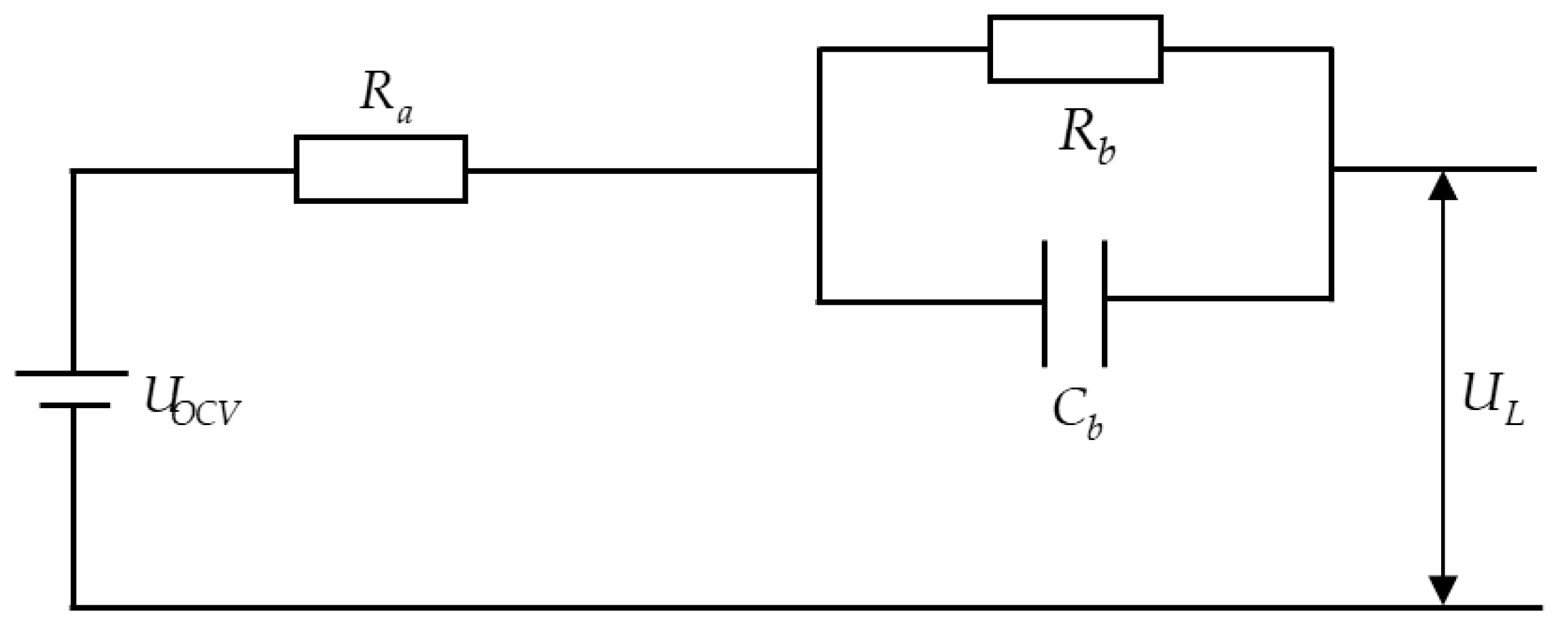
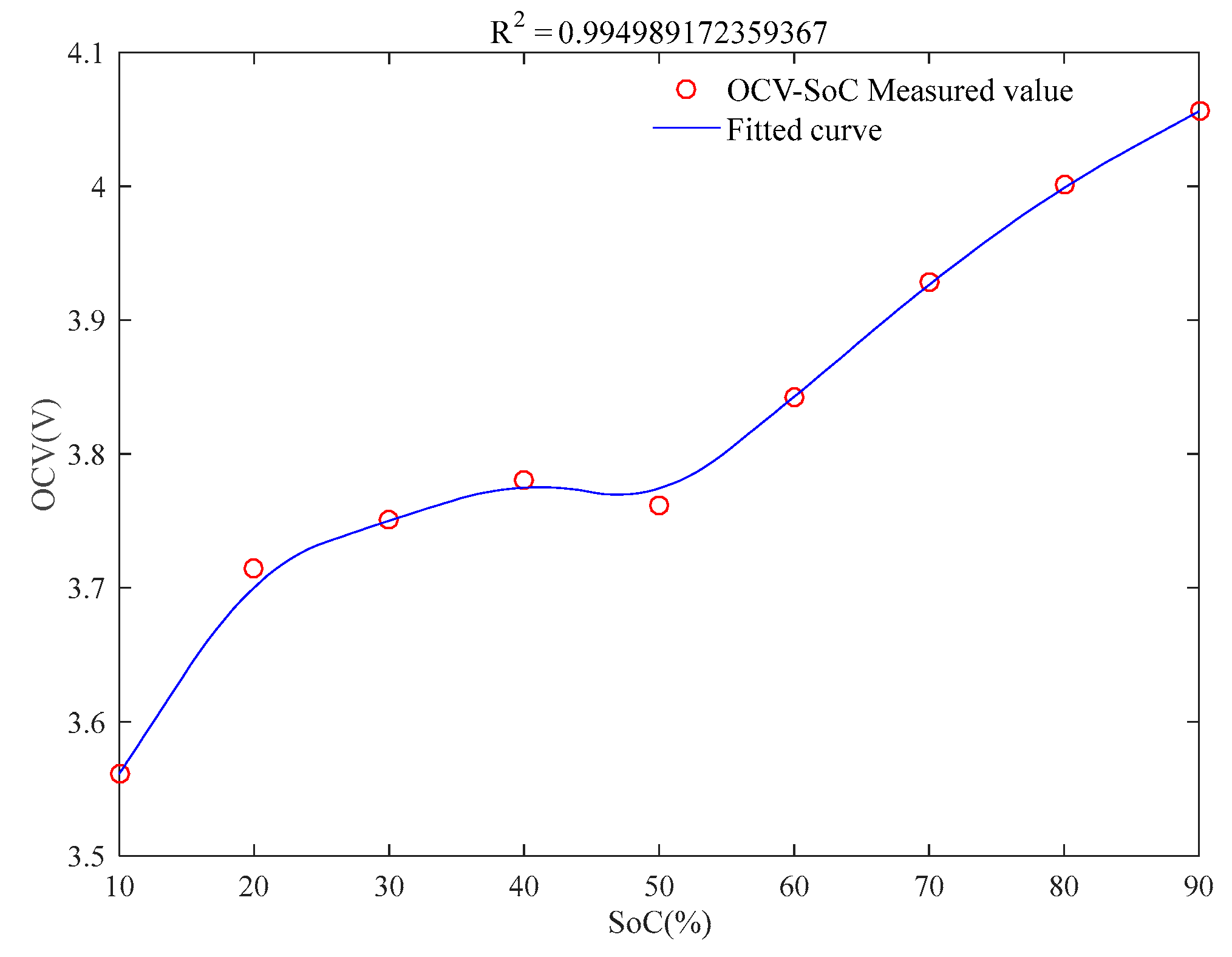
2. Battery State Space Model
3. Algorithm Design
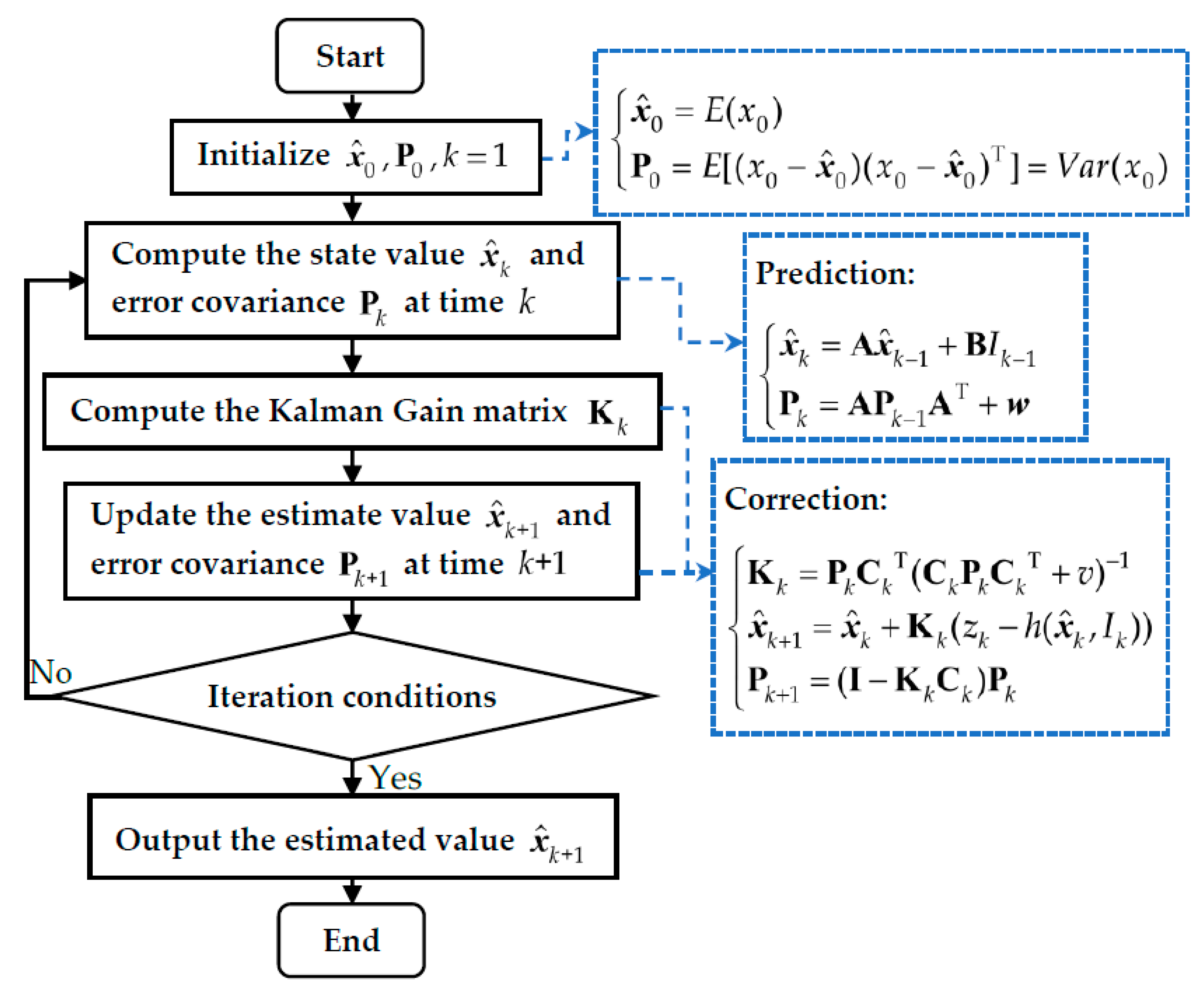
3.1. EKF Algorithm
3.2. BP Neural Network
3.2.1. Data Sources and Pretreatment
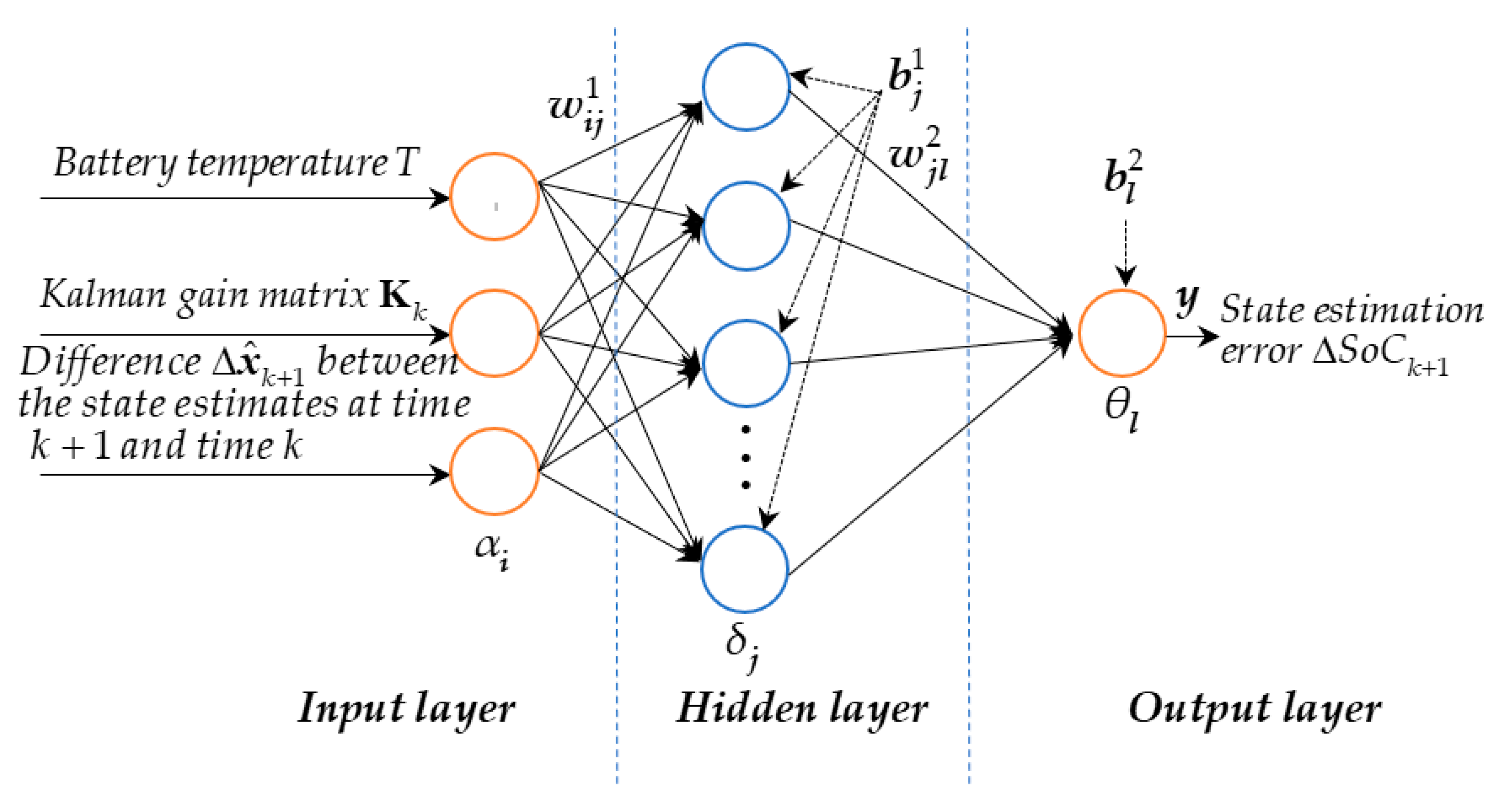
3.2.2. Structure Design of BP Neural Network
3.3. Combination of BP Neural Network Optimized by BBO Algorithm and EKF
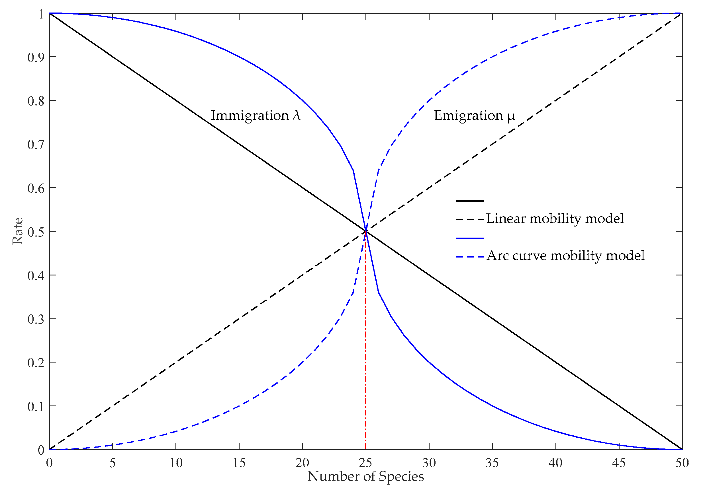
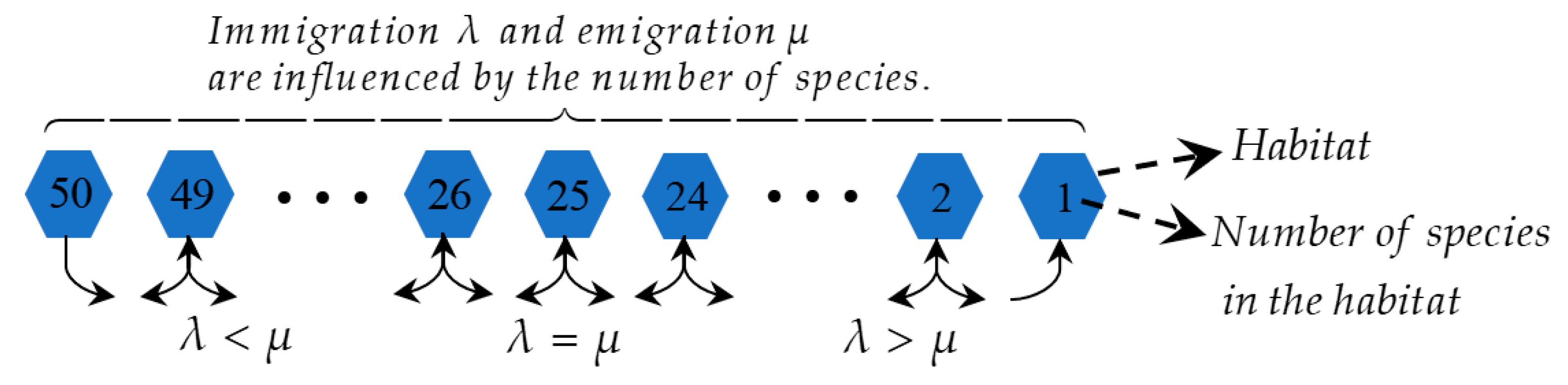
3.3.1. BBO Algorithm
3.3.2. Implementation Process of BBOBP-EKF Algorithm
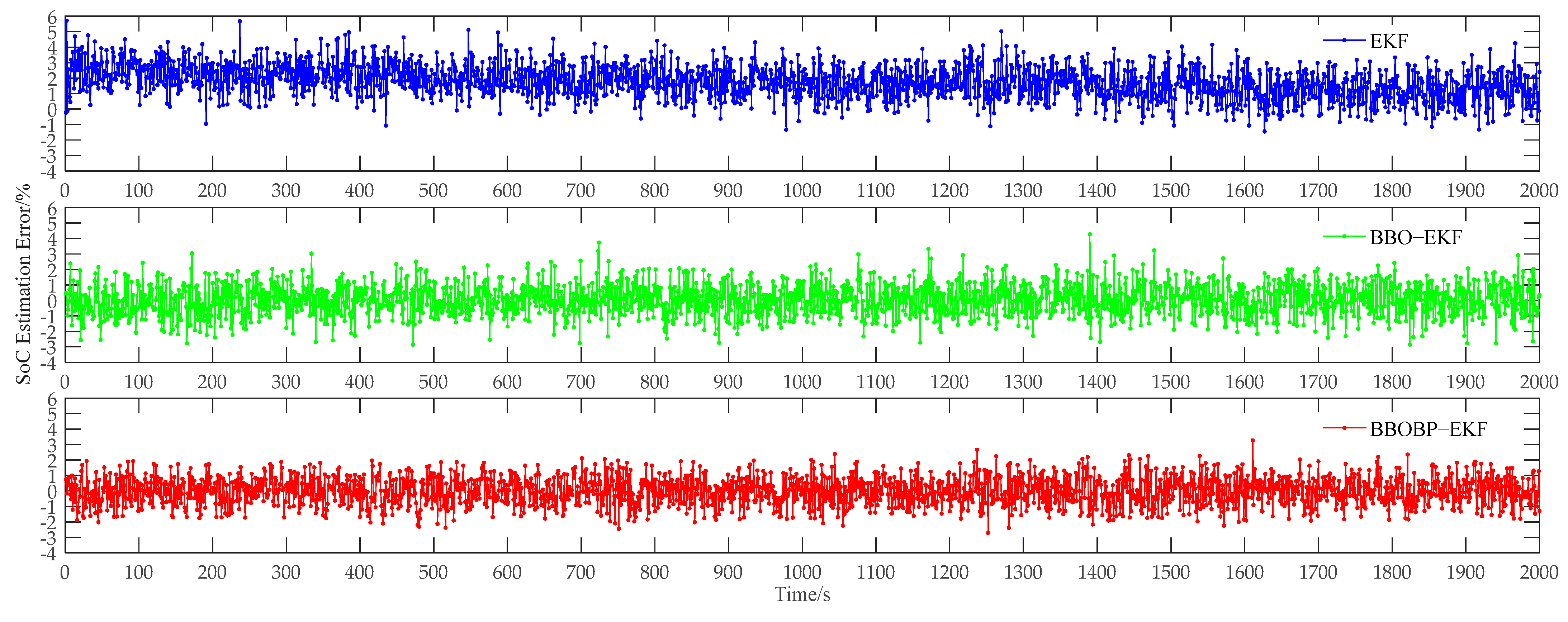
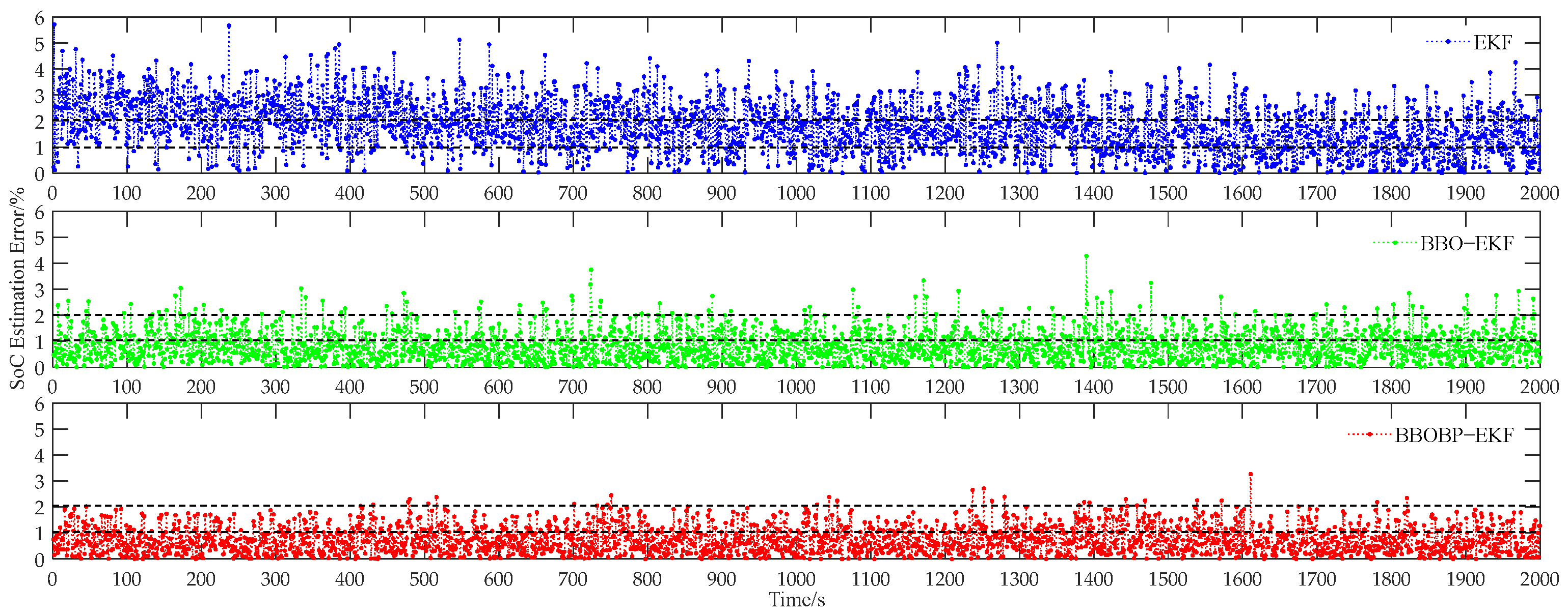
4. Experimental Results and Analysis
5. Conclusions
Author Contributions
Funding
Institutional Review Board Statement
Informed Consent Statement
Data Availability Statement
Conflicts of Interest
Abbreviations
| EVs | Electric vehicles |
| SoC | State of charge |
| OCV | Open-circuit voltage |
| KF | Kalman filter |
| EKF | Extended Kalman filter |
| DEKF | Dual extended Kalman filter |
| AEKF | Adaptive extended Kalman filter |
| LiB | Lithium batteries |
| BPNN | Backpropagation neural network |
| BBO | Biogeography-based optimization |
| EM | Electrochemical model |
| EIM | Electrochemical impedance model |
| ECM | Equivalent circuit model |
| LMM | Linear mobility model |
| ACMM | Arc curve mobility model |
| HIS | Habitat suitability index |
| SIV | Suitability index variables |
References
- Lu, L.; Han, X.; Li, J.; Hua, J.; Ouyang, M. A review on the key issues for lithium-ion battery management in electric vehicles. J. Power Sources 2013, 226, 272–288. [Google Scholar] [CrossRef]
- Hannan, M.A.; Lipu, M.S.H.; Hussain, A.; Mohamed, A. A review of lithium-ion battery state of charge estimation and management system in electric vehicle applications: Challenges and recommendations. Renew. Sustain. Energy Rev. 2017, 78, 834–854. [Google Scholar] [CrossRef]
- Lashway, C.R.; Mohammed, O.A. Adaptive battery management and parameter estimation through physics-based modeling and experimental verification. IEEE Trans. Transp. Electrif. 2016, 2, 454–464. [Google Scholar] [CrossRef]
- Snihir, I.; Rey, W.; Verbitskiy, E.; Belfadhel-Ayeb, A.; Notten, P.H.L. Battery open-circuit voltage estimation by a method of statistical analysis. J. Power Sources 2006, 159, 1484–1487. [Google Scholar] [CrossRef]
- Afshar, S.; Morris, K.; Khajepour, A. State-of-charge estimation using an EKF-based adaptive observer. IEEE Trans. Control Syst. Technol. 2018, 27, 1907–1923. [Google Scholar] [CrossRef]
- Fasahat, M.; Manthouri, M. State of charge estimation of lithium-ion batteries using hybrid autoencoder and Long Short Term Memory neural networks. J. Power Sources 2020, 469, 228375. [Google Scholar] [CrossRef]
- Kalman, R.E. A new approach to linear filtering and prediction problems. J. Basic Eng. 1960, 82, 35–45. [Google Scholar] [CrossRef]
- Meng, J.; Ricco, M.; Luo, G.; Swierczynski, M.; Stroe, D.I.; Stroe, A.I.; Teodorescu, R. An overview and comparison of online implementable SoC estimation methods for lithium-ion battery. IEEE Trans. Ind. Appl. 2017, 54, 1583–1591. [Google Scholar] [CrossRef]
- Reif, K.; Unbehauen, R. The extended Kalman filter as an exponential observer for nonlinear systems. IEEE Trans. Signal Process. 1999, 47, 2324–2328. [Google Scholar] [CrossRef]
- Plett, G.L. Extended Kalman filtering for battery management systems of Li PB-based HEV battery packs: Part 1. Background. J. Power Sources 2004, 134, 252–261. [Google Scholar] [CrossRef]
- Plett, G.L. Extended Kalman filtering for battery management systems of Li PB-based HEV battery packs: Part 2. Modeling and identification. J. Power Sources 2004, 134, 262–276. [Google Scholar] [CrossRef]
- Plett, G.L. Extended Kalman filtering for battery management systems of Li PB-based HEV battery packs: Part 3. State and parameter estimation. J. Power Sources 2004, 134, 277–292. [Google Scholar] [CrossRef]
- Lee, S.J.; Kim, J.H.; Lee, J.M.; Cho, B. The State and Parameter Estimation of An Li-ion Battery Using A New OCV-SoC Concept. In Proceedings of the 2007 IEEE Power Electronics Specialists Conference, Orlando, FL, USA, 17–21 June 2007; pp. 2799–2803. [Google Scholar]
- Mastali, M.; Vazquez-Arenas, J.; Fraser, R.; Fowler, M.; Afshar, S.; Stevens, M. Battery state of the charge estimation using Kalman filtering. J. Power Sources 2013, 239, 294–307. [Google Scholar] [CrossRef]
- He, H.; Xiong, R.; Zhang, X.; Sun, F.; Fan, J. State-of-charge estimation of the lithium ion battery using an adaptive extended Kalman filter based on an improved Thevenin model. IEEE Trans. Veh. Technol. 2011, 60, 1461–1469. [Google Scholar]
- Xiong, R.; Gong, X.; Mi, C.C.; Sun, F. A robust state-of-charge estimator for multiple types of lithium ion batteries using adaptive extended Kalman filter. J. Power Sources 2013, 243, 805–816. [Google Scholar] [CrossRef]
- Hu, Y.; Wang, Z. Study on SoC Estimation of Lithium Battery Based on Improved BP Neural Network. In Proceedings of the 2019 8th International Symposium on Next Generation Electronics (ISNE), Zhengzhou, China, 9–10 October 2019; pp. 1–3. [Google Scholar]
- Tian, D.; Li, L.; Yang, Y. Research on SoC estimation based on improved BP-EKF algorithm. Chin. J. Power Sources 2020, 44, 1274–1278. [Google Scholar]
- Gao, Y.; Ji, W.; Zhao, X. SoC Estimation of E-Cell combining BP neural network and EKF algorithm. Processes 2022, 10, 1721. [Google Scholar] [CrossRef]
- Simon, D. Biogeography-based optimization. IEEE Trans. Evol. Comput. 2008, 12, 702–713. [Google Scholar] [CrossRef]
- Liu, G.; Lu, L.; Fu, H.; Hua, J.; Li, J.; Ouyang, M.; Wang, Y.; Xue, S.; Chen, P. A comparative study of equivalent circuit models and enhanced equivalent circuit models of lithium-ion batteries with different model structures. In Proceedings of the 2014 IEEE Conference and Expo Transportation Electrification Asia-Pacific (ITEC Asia-Pacific), Beijing, China, 31 August–3 September 2014; pp. 1–6. [Google Scholar]
- Wang, Q.; He, Y.; Shen, J.; Hu, X. State of charge-dependent polynomial equivalent circuit modeling for electrochemical impedance spectroscopy of lithium-ion batteries. IEEE Trans. Power Electron. 2017, 33, 8449–8460. [Google Scholar] [CrossRef]
- Nemes, R.; Ciornei, S.; Ruba, M.; Hedesiu, H.; Martis, C. Modeling and simulation of first-order Li-Ion battery cell with experimental validation. In Proceedings of the 2019 8th International Conference on Modern Power Systems (MPS), Cluj Napoca, Romania, 21–23 May 2019; pp. 1–6. [Google Scholar]
- Zhang, X.; Lu, J.; Yuan, S.; Yang, J.; Zhou, X. A novel method for identification of lithium-ion battery equivalent circuit model parameters considering electrochemical properties. J. Power Sources 2017, 345, 21–29. [Google Scholar] [CrossRef]
- Shi, Y.; Ahmad, S.; Tong, Q.; Lim, T.M.; Wei, Z.; Ji, D.; Eze, C.M.; Zhao, J. The optimization of state of charge and state of health estimation for lithium-ions battery using combined deep learning and Kalman filter methods. Int. J. Energy Res. 2021, 45, 11206–11230. [Google Scholar] [CrossRef]
- He, Z.; Li, Y.; Sun, Y.; Zhao, S.; Lin, C.; Pan, C.; Wang, L. State-of-charge estimation of lithium ion batteries based on adaptive iterative extended Kalman filter. J. Energy Storage 2021, 39, 102593. [Google Scholar] [CrossRef]
- Fan, B.; Ren, S.; Luo, J. Research on relationship between SoC and OCV of lithium ion battery under actual application conditions. Chin. J. Power Sources 2018, 42, 641–644. [Google Scholar]
- Mcclelland, J.L.; Rumelhart, D.E.; PDP Research Group. Parallel Distributed Processing; MIT Press: Cambridge, MA, USA, 1986. [Google Scholar]
- Ma, H.; Lipu, M.S.H.; Hussain, A.; Mohamad, H.S.; Afida, A. Neural network approach for estimating state of charge of lithium-ion battery using backtracking search algorithm. IEEE Access 2018, 6, 10069–10079. [Google Scholar]
- Wang, S.; Ma, H.; Dou, J.; Zhang, Y.; Li, S.; Hu, L. Estimation of lithium-ion battery state of charge based on UGOA-BP. Energy Storage Sci. Technol. 2022, 11, 258–264. [Google Scholar]
- Zhang, Y.; Gu, X. Biogeography-based optimization algorithm for large-scale multistage batch plant scheduling. Expert Syst. Appl. 2020, 162, 113776. [Google Scholar] [CrossRef]
- Zhang, Z.; Gao, Y.; Zuo, W. A dual biogeography-based optimization algorithm for solving high-dimensional global optimization problems and engineering design problems. IEEE Access 2022, 10, 55988–56016. [Google Scholar] [CrossRef]
- Xu, P.; Chen, S.; Yu, X.; Zhang, L. Developing a novel hybrid biogeography-based optimization algorithm for multilayer perceptron training under big data challenge. Sci. Program. 2018, 2018, 2943290. [Google Scholar]
- Zhang, X.; Wen, S.; Wang, D. Multi-population biogeography-based optimization algorithm and its application to image segmentation. Appl. Soft Comput. 2022, 124, 109005. [Google Scholar] [CrossRef]


| Error Taking Absolute Value Interval/% | EKF | BP-EKF | BBOBP-EKF |
|---|---|---|---|
| 459 | 1331 | 1412 1 | |
| 726 | 574 | 554 | |
| 815 | 95 | 34 |
| Index | Minimum Error /% | Maximum Error/% | Mean Absolute Value of Error/% | Error Variance/% |
|---|---|---|---|---|
| EKF | 1.6421 × 10⁻³ | 5.7156 | 1.8099 | 1.1731 |
| BP-EKF | 9.9855 × 10⁻⁴ | 4.2849 | 0.8207 | 1.0498 |
| BBOBP-EKF | 1.7112 × 10⁻⁴ 2 | 3.2658 | 0.7483 | 0.9443 |
Disclaimer/Publisher’s Note: The statements, opinions and data contained in all publications are solely those of the individual author(s) and contributor(s) and not of MDPI and/or the editor(s). MDPI and/or the editor(s) disclaim responsibility for any injury to people or property resulting from any ideas, methods, instructions or products referred to in the content. |
© 2023 by the authors. Licensee MDPI, Basel, Switzerland. This article is an open access article distributed under the terms and conditions of the Creative Commons Attribution (CC BY) license (https://creativecommons.org/licenses/by/4.0/).
Share and Cite
Liu, X.; Zhang, X. State of Charge Estimation for Power Battery Using Improved Extended Kalman Filter Method Based on Neural Network. Appl. Sci. 2023, 13, 10547. https://doi.org/10.3390/app131810547
Liu X, Zhang X. State of Charge Estimation for Power Battery Using Improved Extended Kalman Filter Method Based on Neural Network. Applied Sciences. 2023; 13(18):10547. https://doi.org/10.3390/app131810547
Chicago/Turabian StyleLiu, Xiaoyu, and Xiang Zhang. 2023. "State of Charge Estimation for Power Battery Using Improved Extended Kalman Filter Method Based on Neural Network" Applied Sciences 13, no. 18: 10547. https://doi.org/10.3390/app131810547
APA StyleLiu, X., & Zhang, X. (2023). State of Charge Estimation for Power Battery Using Improved Extended Kalman Filter Method Based on Neural Network. Applied Sciences, 13(18), 10547. https://doi.org/10.3390/app131810547