Abstract
The elastic-damping properties of the rubber track structure can have a significant impact on the running gear performance of lightweight mobile robots. Taking these properties into account is particularly important for modeling obstacle negotiation and estimating the robot’s driving force. The article presents track susceptibility identification using both static and dynamic tests. The experimental results were used to validate the multi-body dynamics model of the rubber track for three modeling methods and for three track link number model variants. The methods and variants were compared by the accuracy of the susceptibility parameters obtained using them. The impact of the modeling methods on the track bending resistance simulations was also checked.
1. Introduction
With the development of technology, mobile robots and UGVs (Unmanned Ground Vehicles) are gaining more and more widespread use in many areas of life [1,2]. Their main capability is to directly replace humans in hazardous work environments. To achieve the necessary functionality, they are required to have an adequate mobility level for the working conditions, effectiveness in task performance [3], and sufficient energy reserve for the expected working time [4].
In order to increase mobility, robots and UGVs are often equipped with tracked running gear [5,6]. Compared with wheeled traction systems, tracked systems are characterized by lower pressures, a higher ability to overcome terrain with low load capacity, the ability to develop higher traction forces with less slip, and a greater ability to overcome terrain obstacles [7]. More and more often, instead of metal tracks, rubber tracks are used. They allow for driving on both paved roads and off-roads while ensuring quieter operation [8], a longer service life, and lower operating costs [9], as well as better traction characteristics and an advantageous distribution of ground pressure [10,11], typical for tracks. For these reasons, they can be increasingly used in low-speed transport vehicles and agricultural tractors of various sizes, where they replace wheeled chassis [10,11,12,13,14].
Experimental and simulation studies in the field of rubber track applications focus mainly on the prediction of traction forces and rolling resistance on deformable soils, taking into account the principles of terramechanics [15,16,17]. These studies show the high compatibility of heavy vehicle models; using them to model light robots and UGVs does not always bring satisfactory results [18]. Similar problems occur when modeling the energy efficiency of driving. Experimental studies show that the resistance and energy consumption, especially of lightweight robots, can be relatively higher than in the case of classic heavy-tracked vehicles with metal tracks [19,20,21]. The rolling resistance coefficient may be the main component of energy loss. Even on non-deformable surfaces, it may exceed 20% [3,22].
Research [19,23] indicates factors that have a significant impact on the internal motion resistance of rubber track running gear: track scrolling speed, diameters of driving, idler, and road wheels, as well as stiffness and damping of the track belt, depending on the type of rubber and structure of the track belt. These properties not only increase the track bending resistance but also cause the track belt to heat up and increase its temperature [24,25]. This may change its stiffness, lead to track elongation and shedding while driving, cause devulcanization, and accelerate the degradation of the track structure [26]. In addition, the stiffness of the track belt (its susceptibility to deformation) and the track tension have a dominant effect on the contact with the ground. Increased track-terrain contact improves ground pressure, tractive forces, and the general ability to overcome obstacles [17], which also depends on the applied running gear solutions [27,28,29]. It is therefore advisable to take these factors into account in the track modeling process, especially in systems with complex kinematics, moving on rough surfaces, and overcoming obstacles.
2. Track Susceptibility in Simulation Models
In order to properly shape the running gear, simulation tests [27,30,31,32,33,34] are widely used. They make it possible to estimate the drive torques necessary to overcome the motion resistance, obstacle negotiation ability [35], maneuver performance resistance [33], and energy consumed by the robot [20].
Despite the impact of rubber track susceptibility on many aspects of the robot’s functionality, it is not always taken into account. In fast real-time simulations, in order to shorten the calculation time, the structure of the track belt may be omitted or simplified [36,37]. Running gear is presented as a system consisting only of driving wheels. The belt adds to the hull weight. To increase the accuracy of the track-terrain contact surface, there are models where the shape of the tracked running gear is obtained by using an increased number of overlapping wheels to form an almost continuous contact surface with the ground [33,38]. An alternative solution is also to use the non-deformable track model [35,39]. It allows the track to perform on the ground, developing tractive force, but track deformation in reaction to the ground is impossible. This model allows for relatively quick determination of the parameters of driving straight, negotiating small, simple obstacles, and even turning with a fixed radius. The problem, however, may be situations of point contact with the ground, e.g., curb or stair climbing [37]. This type of model is also used to predict the motion parameters of robots when performing maneuvers [33].
The track model, taking into account its deformation ability, can be achieved by the coupled multibody dynamics-finite elements method model [40] or the finite element method [41,42]. A model using a system of wheels and a track belt with a structure divided into a finite number of elements was used, e.g., in the research [42] of the rubber-tracked running gear of a farm tractor. Considering the elasticity of the rubber belt, its deflection under its own weight was used to model parameter identification. By using finite elements, it is possible to give the elastomer material non-linear, hyperelastic properties. In this way, its deformations and stresses while driving can be reflected with high accuracy. The disadvantage of the method is its long simulation time. Therefore, despite the possibility of using the FEM method in dynamic simulations, it will not always be fully practical.
Another track modeling method is to digitize the belt into a finite number of elements (links) connected with each other by constraints (joints), defining its motions by restricting degrees of freedom [43,44,45]. This method is widely used in metal track modeling [28,46]. It allows deformation of the track in accordance with the adopted constraints as well as a more accurate verification of which of its elements remain in contact with the ground. It is especially useful when simulating overcoming terrain roughness. Three connection methods are most often used between track links: kinematic joints, force constraints, and constraints with plastic deformation ability [44].
The simplest type of track-link connection is one with kinematic constraints. They provide movement in an established angular range, but they do not reflect any forces occurring in the constraint. This method was used in research on heavy vehicle dynamics [28,45,46,47]. The simulations and experiment results for acceleration when driving over small obstacles were compared [48]. The simulation data is compatible with experiments at low speeds. At higher speeds, the omission of the damping constraint properties resulted in too high simulated vertical vehicle body acceleration. This indicates the need to take into account the elastic-damping properties of the track belt constraints.
These properties may be described by general force constraints between track links. In the available research models, bushing connections (which define a six-degree-of-freedom force relationship between two parts) are used for this purpose [49]. The forces in three axes and torques in three planes are often characterized by damping and stiffness coefficients (factors). Typically, similar proportions of stiffness and damping coefficients are maintained. The coefficients used to have fixed, constant values, but they are not always published [27,50].
Force connections were used, among others, in simulations of a light agricultural tractor [49]. Due to track discretization, the individual ground reaction force for each link and the sinkage were calculated. The values of the parameters of damping and stiffness between the track elements were selected by comparing the simulation-obtained track belt shape to the real track belt set freely on the ground. The force connection was also successfully used in simulations of rubber-tracked running gears of light mobile robots when overcoming terrain unevenness [27].
Stiffness and damping parameters between the track segments were usually selected on the basis of trial and error during simulations and observation of the static deflection of the track belt. However, the elastic-damping properties also vary with the deformation radius and the scrolling speed of the tracks [23]. Statically determined parameters may therefore lead to significant errors during the track belt performance simulation. Reliable studies of tracked running gear dynamics require the development of a track belt model using experimentally determined stiffness and damping properties of track belts in dynamic tests.
3. Track Belt Model
The elastomer track belt simulation model was made in the ADAMS MBD simulation program [51]. The track belt was considered a flat system composed of link-type elements. Furthermore, links were joined by general force vector constraints, enabling rotation in the transverse axis Z (Figure 1). The forces in the connection were characterized by the longitudinal, transverse, and angular stiffness and damping values (Figure 1). Forces and torque occurring in the constraints were determined according to the equations:
where is the rotation angle of the link axes, are displacements of the connected elements, are longitudinal and transverse stiffness, is the angular stiffness, are the damping values on the X and Y directions, and is rotational damping in the transverse Z axis.
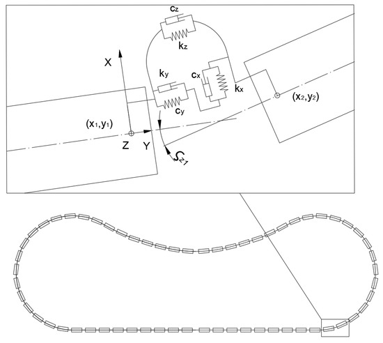
Figure 1.
Rubber track links constraint scheme.
The values of the stiffness and damping coefficients depend on the length and number of links representing the track belt; therefore, three track model variants were developed:
- Variant where links and grouser quantities are equal (38-element variant—E38);
- Variant with 1.5 times increased link quantity (56-element variant—E56);
- Variant with twice the link quantity (76 element variant—E76).
Based on the rubber tracks modeling publication analysis, the coefficients of longitudinal and transverse stiffness and damping were determined as = 100,000 N/mm and = 1000 N/mm/s. High values of these coefficients significantly limited the possibility of longitudinal displacements of the track links. Therefore, the coefficients of angular stiffness and damping mainly affected the track’s susceptibility and its deformation ability. In order to determine the exact values of these parameters, experimental tests were carried out.
4. Identification Tests
4.1. Methodology
The experimental test subject was a rubber track (Figure 2) from an off-road platform, the DTV Shredder. The platform weighed about 115 kg; moreover, it was designed to carry a person (an extra 100 kg of load). The total length of the track was L = 2450 mm, the belt width was B = 160 mm, and its thickness A = 8 mm. The single belt weighted m = 6.4 kg. Due to its off-road adaptation, the track belt was equipped with 38 rubber grousers (with a pitch p = 64.5 mm).
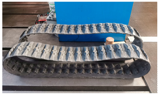
Figure 2.
Rubber tracks of the DTV Shredder platform.
The measurement was carried out using the ARAMIS high-resolution 3D optical system, which allows measuring the displacements of the selected points. The vision system consisted of two cameras with a resolution of 4096 × 3000 pixels and a frequency of 25 Hz. 38 point markers were placed around the circumference of the belt and recorded by a camera system [52]. The experiment procedure was divided into two consecutive tests:
- a static test in which belt deflections were measured;
- a dynamic test, which assumed the recording of track oscillations under a load.
The measurements included two track belts (track 1 and track 2). Each measurement was repeated for each track four times, every time rewinding the belt ¼ its length. Figure 3 shows the exemplary measurement image obtained using the ARAMIS system.
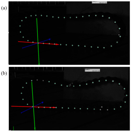
Figure 3.
The rubber track measurement recorded in the optical system during: (a) static test and (b) dynamic test.
4.2. Static Test
During the static test, the track was placed in equilibrium on a flat surface (Figure 4a) only loaded with its weight. The static height (Hs) of point A (Figure 4a) and the width (Ws) were measured. The results are presented in Table 1. The mean values were used as the criterion for the validation of stiffness and damping parameters in the simulations. The greatest result deviation from the mean value was 15 mm, which is about 4.5%. In turn, the largest Ws result deviation was smaller than 1% of its calculated mean value.
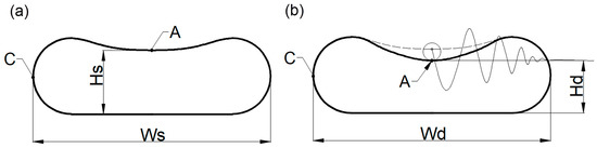
Figure 4.
Track belt measurements scheme in: (a) static test; (b) dynamic test.

Table 1.
Results of experimental static and dynamics tests.
4.3. Dynamic Test
The dynamic test involved forcing belt oscillation by loading it at point A (Figure 4b) with a 1.3 kg weight roller. The track oscillation plot of point A on the vertical axis, the final height Hd, and the final width Wd of the deformed track (Figure 4b) were recorded. On this basis, the following parameters were determined:
- track deformation height Hd after loading;
- track deformation width Hd after loading;
- time period T of track oscillation;
- logarithmic decrement Λ of track oscillation (which describes the level of oscillation damping provided by the material and structure of the track belt). Parameters are calculated according to the equation:
The three exemplary oscillation plots are presented in Figure 5. The parameters determined on their basis (Table 1) were not as compatible as the static test results. The greatest result deviation referred to the logarithmic decrement Λ, and it reached almost 15% of the mean value. The remaining deviations were 7% for height Hd, 1% for width Wd, and 2% for time period T. The mean values of these parameters were used to validate the simulation model dumping and stiffness coefficients.
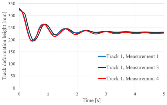
Figure 5.
The three exemplary track oscillation plots, recorded in dynamic test of track 1.
5. Model Validation
In order to determine the parameters of angular stiffness and angular damping , computer simulations were carried out. The track belt was formed into a circle and lowered onto a flat surface. After the track belt was formed by its own weight, the static test parameters were determined. Furthermore, the tracks were loaded with 1.3 kg of weight, and the oscillation parameters were determined. Comparing simulation parameters from static and dynamic tests with the experimental results, stiffness and damping in track belt constraints were set up (Figure 6).
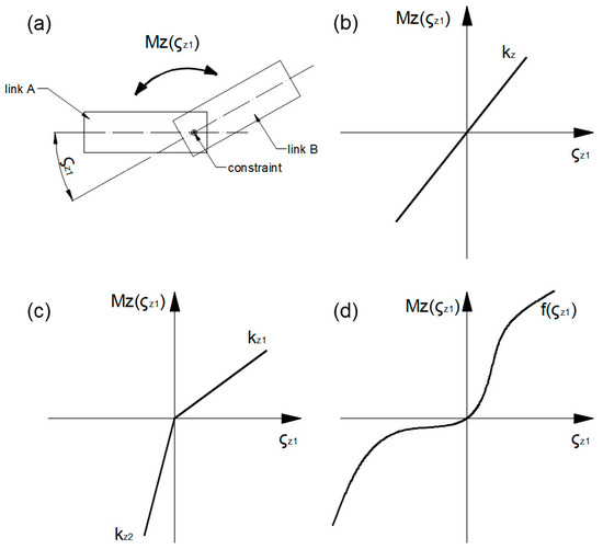
Figure 6.
Track links constraint scheme (a), and the constraint torque-links of angular stiffness definition methods: (b) Method I; (c) Method II; (d) Method III.
In order to match the simulation results with the experimental tests as precisely as possible, three methods of angular stiffness definition in the constraints (Figure 6a) were compared:
- Method I: constant stiffness value regardless of the angle (Figure 6b);
- Method II: bivalent stiffness—two different values , for bending track belt inwards and outwards (Figure 6c);
- Method III: variable stiffness value in the whole range of angles . In this method, instead of the stiffness coefficient , the torque—rotation angle characteristic is used in constraints as a nonlinear function (Figure 6d).
The constraint modeling methods were compared with each other on the basis of their relative errors. In addition, it was established whether the modeling method would affect the simulation-determined track belt bending resistance. For each method, the drive torque needed to scroll the track at a constant speed between a drive wheel and an idler without contact with the ground was determined.
5.1. Track Modeling Using Constant Stiffness Constraints
The angular stiffness coefficients for three track variants (E38, E56, and E76) were selected by adjusting the achieved value of the height Hs with the static test results. With an increase in the stiffness coefficient, the values of the heights Hs and Hd also increased. The damping coefficient was adjusted on the basis of the logarithmic decrement Λ so that its simulation-derived value was within the 10% accuracy range with the dynamic test experimental results. By changing the damping values, it was possible to adjust the oscillation amplitudes. A comparison of the oscillation plots obtained in the dynamic tests and simulations is shown in Figure 7. The values of the stiffness and damping parameters for three variants of the track model and the obtained simulation results are presented in Table 2.
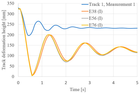
Figure 7.
The track oscillations plots comparison: experimental measurement and simulation results from constant stiffness constraint model in variants E38, E56 and E76.
Table 2.
Simulations results from constant stiffness constraint model (I) in variants E38, E56, E76.
Simulations indicated that regardless of the number of segments used for the track belt model, the obtained oscillation parameters remained similar. The use of constant stiffness resulted in an oscillation time period twice as long as the experimental one. In addition, the height Hd obtained in the simulations turned out to be almost two times lower than the experimental measurements. These differences may indicate that the constant value of the stiffness coefficient is insufficient to describe the susceptibility of the rubber belt.
During the simulations, the range of angles between the modeled track links was also determined. Connections with the largest amplitudes of rotation angles are marked in Figure 4 with the letters A and C. The angle values obtained under these constraints are shown in Table 3. As the number of links increases, the range of rotation angles decreases.
Table 3.
Ranges of rotation angle in selected connections of the track belt links (Figure 4) in constant stiffness constraint model in variants E38, E56 and E76.
5.2. Track Modeling Using Bivalent Stiffness Constraints
Constraints with two stiffness coefficient values were applied in the rubber track model: for positive rotation angles and for negative ones. Increasing the stiffness in the positive range caused a significant oscillation period reduction. By limiting the possibility of track belt deflection, its upper part (point A) oscillated faster. In order to obtain oscillation period results similar to those from the experiment, the coefficient needed to be increased almost 15 times (in relation to the value of the stiffness constant). This change in stiffness also caused an increase in the height of Hd and significantly reduced the oscillation amplitudes. As a result, it was necessary to modify the damping coefficient , so that the logarithmic decrement values were consistent with the experimental test results. The parameter remained at the same value as in the constant stiffness model. This parameter was responsible for the deflection of the side parts of the track (point C), so its stiffness was determined properly to obtain the height Hs. The determined values of stiffness and damping, as well as the parameters of the simulation tests, are presented in Table 4. A comparison of the oscillation plots obtained in the dynamic tests and bivalent stiffness constraint simulations is shown in Figure 8.
Table 4.
Simulations results from bivalent stiffness constraint model (II) in variants E38, E56, E76.
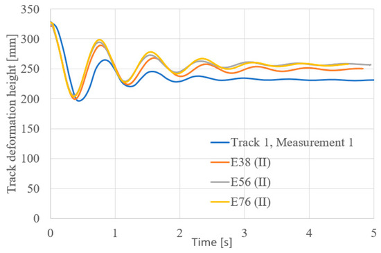
Figure 8.
The track oscillations plots comparison: experimental measurement and simulation results from bivalent stiffness constraint model in variants E38, E56 and E76.
The use of a bivalent stiffness model resulted in a significant improvement in the consistency of the simulations and experiments, especially in terms of the time period.
Increased stiffness caused a decrease in the point A (Figure 4) rotation angle range (Table 5). Such a powerful stiffening of the track belt was an adverse phenomenon. Visualizations did not agree with the experimental track’s dynamic deflection in terms of its overall shape. The simulation-obtained height Hd exceeded the height from the dynamic test. Furthermore, to obtain logarithmic decrement results consistent with the experimental results, the damping coefficient needed to be lowered at least two times.
Table 5.
Ranges of rotation angle in selected conscontraints of the track belt (Figure 4) in bivalent stiffness constraint model in variants E38, E56 and E76.
5.3. Track Modeling Using Variable Stiffness Constraints
In the variable stiffness model, the torque occurring in each constraint was applied depending on the rotation angle value. The constraint torque-links rotation angle characteristic plot was assumed after many simulation attempts. They were able to shape the results of the simulation tests by changing the torque values in the different angle ranges. The determined function, divided into modified ranges, is presented in Figure 9.
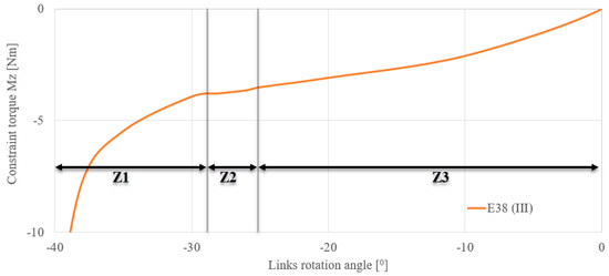
Figure 9.
The constraint torque-links rotation angle characteristics determined for E38 (III) track simulation variant.
The negative part of the function plot was divided into three ranges: Z1, Z2, and Z3 (Figure 9). The constraint torque in the Z1 range determined the maximum rotation angle that occurred in the simulation. Shaping the function plot in this range allowed to set the height Hd. In order to achieve the expected Hs value, it was necessary to modify the Z2 angle range (Figure 9). By reducing the curve inclination, the difference between Hd and Hs values increased. At the same time, this procedure reduced the oscillation time period. In order to balance the phenomenon for the Z3 small angles, the torque function was shaped more inclined. Increased stiffness in the Z3 range allowed for the proper time period to occur and also maintained the correct overall geometric shape of the deflected track. The torque values in the positive angle range (Figure 10) were determined to be more inclined than in the range of Z2 and Z3, but the difference between the positive and negative angle ranges of function inclination was not as high as in the bivalent stiffness simulation method (II).
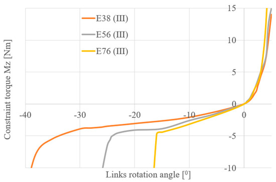
Figure 10.
Comparison of constraint torque in the segment rotation angle function plots assumed for variants E38, E56 and E76.
Using these steps, stiffness characteristics and damping values for three variants of the track model were assumed. They are presented in Figure 10. The oscillation plots for all three variants of simulations are presented in Figure 11. Simulation static and dynamic test parameters and assumed damping coefficients are presented in Table 6, and the obtained rotation angle ranges are described in Table 7.
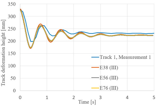
Figure 11.
The track oscillations plots comparison: experimental measurement and simulation results from variable stiffness constraint model in variants E38, E56 and E76.
Table 6.
Simulations results from variable stiffness constraint model (III) in variants E38, E56, E76.
Table 7.
Ranges of rotation angle in selected constraint s of the track belt (Figure 4) in variable stiffness model in variants E38, E56 and E76.
Using the variable stiffness model, the simulation results were compatible with the experiments. The maximum difference between the values obtained in simulations and the mean value of the experiment results does not exceed 10% of the experimental value in any of the parameters.
6. Discussion
6.1. Relative Errors Comparison of Modeling Methods
Three methods of track modeling simulation were compared in terms of relative error for the mean value of the experimental results. The error values of simulation-determined parameters are presented in Table 8. The height’s Hd and logarithmic decrement were stiffness and damping parameters adjusting criteria. Other parameters indicated the compatibility level of the results. The track deformation width errors Ws and Wd did not change significantly depending on the adopted simulation methods and variants. They amounted to no more than 2%.
Table 8.
The relative error values of simulation results.
The first method of the simulations (I) was the one most burdened with the time period error. The use of bivalent stiffness (II) reduced the time period relative error ten times and the height Hd relative error four times compared with the first simulation method (I). The use of the variable stiffness method (III) allowed for the most accurate model of susceptibility tests. The largest error in this case (apart from the criteria parameters) concerns the time period, which amounted to 4%. There were no significant differences between the three simulation variants. By selecting the correct values of the damping and stiffness coefficients, it was possible to obtain almost the same plots of oscillation for a track composed of longer and shorter links.
The use of method I, which is characterized by model simplicity and low calculation time, allows achieving satisfactory results only in static tests. It may be appropriate for vehicle static stability tests. The use of the second method slightly complicates the computational model but significantly improves the accuracy of dynamic test results. This method can be a good compromise between complex track stiffness characteristics and its constant value assumption. In this method of simulation (II), it might be possible to observe reliable track deflection and its oscillations while driving. The use of the third method (III) will extend the model calculation time, but it allows the most accurate prediction of both static and dynamic track performance. It can be useful for accurately determining the parameters of track deformation or energy dissipation in rubber track running gear simulations. However, accurate stiffness characteristics will only be valid for a specific construction and type of track belt, so they will not be universal.
6.2. Track Belt Bending Resistance Simulations
In order to confirm the impact of the track modeling method on the bending resistance force, additional simulations of the E56 variant were carried out. The plot of the drive torque necessary to rewind the crawler track stretched between the drive and idler wheels (Figure 12a) with diameters of 300 mm was determined. The drive wheel was accelerated to a 5 rad/s angular speed in 1 s and then kept constant at 5 rad/s. The driving torque plot for three methods of track modeling is shown in Figure 12b.
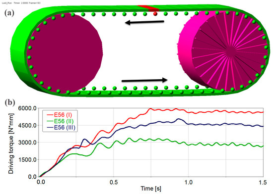
Figure 12.
Track belt bending resistance simulations: (a) simulation model; (b) simulation results driving torque plots for three modeling methods.
Based on the obtained driving torque plots, it can be seen that the track constraints modeling method has an impact on the torque needed to bend the rubber track while scrolling. The driving torque used to scroll track in the E56 (II) bivalent stiffness model was two times lower than in the E56 (I) constant stiffness model. Such differences may be related mainly to different assumed damping coefficients.
7. Conclusions
The method of testing the rubber track susceptibility proposed in the article allowed the determination of stiffness and damping parameters for three methods of link connection modeling. Comparing the relative errors of simulation results, modeling methods were assessed. The more developed the stiffness description, the more accurate the results were. In the future, it is also planned to extend the model with a non-linear damping description. It was also found that by increasing the link number even twice, no significant impact on the test result accuracy was achieved. A different number of model elements, however, determined higher stiffness and damping coefficients.
A significant impact of the modeling method on the drive torque spent on rubber belt bending was also noted. However, further research is needed to verify the belt bending resistance torque and evaluate the simulation models in terms of their actual values. Future experimental research will therefore be concerned with examining the energy consumption of running gear equipped with rubber tracks. Based on the results, it will be possible to extend the track model to account for the more complex damping characteristics of the track link constraints. The developed rubber track model will be used in simulations of lightweight tracked mobile robots in order to predict their energy consumption and ability to overcome obstacles.
Author Contributions
Conceptualization, P.K. and M.J.Ł.; methodology, P.K.; software, D.S. and P.K.; validation, D.S.; formal analysis D.S.; investigation, D.S. and M.J.Ł.; resources, D.S. and P.K.; data curation, D.S.; writing D.S., M.J.Ł. and P.K.; visualization D.S.; supervision M.J.Ł.; project administration M.J.Ł.; funding acquisition, M.J.Ł. All authors have read and agreed to the published version of the manuscript.
Funding
This work was financed/co-financed by the Military University of Technology under research project UGB 22-830/2023.
Institutional Review Board Statement
Not applicable.
Informed Consent Statement
Not applicable.
Data Availability Statement
Not applicable.
Conflicts of Interest
The authors declare no conflict of interest.
References
- Gage, D.W. UGV History 101: A Brief History of Unmanned Ground Vehicle (UGV) Development Efforts; Naval Ocean Systems Center: San Diego, CA, USA, 1995; 13p. [Google Scholar]
- Rubio, F.; Valero, F.; Llopis-Albert, C. A Review of Mobile Robots: Concepts, Methods, Theoretical Framework, and Applications. Int. J. Adv. Robot. Syst. 2019, 16, 1–22. [Google Scholar] [CrossRef]
- Lopatka, M.; Rubiec, A.; Przybysz, M.; Krogul, P. State of the Art of Working Capabilities and Mobility of Robots—“Medium Platform (Weight 800 Kg)” Project Report; Military University of Technology: Warsaw, Poland, 2014. (In Polish) [Google Scholar]
- Farooq, M.U.; Eizad, A.; Bae, H.-K. Power Solutions for Autonomous Mobile Robots: A Survey. Rob. Auton. Syst. 2023, 159, 104285. [Google Scholar] [CrossRef]
- Bruzzone, L.; Nodehi, S.E.; Fanghella, P. Tracked Locomotion Systems for Ground Mobile Robots: A Review. Machines 2022, 10, 648. [Google Scholar] [CrossRef]
- Lopatka, M. UGV for Close Support Dismounted Operations—Current Possibility to Fulfil Military Demand. In Challenges to National Defence in Cotemporary Geopolitical Situation; Ministry of National Defence Republic of Lithuania: Vilnius, Lithuania, 2020; pp. 22–24. [Google Scholar] [CrossRef]
- Wong, J.Y.; Huang, W. “Wheels vs. Tracks”—A Fundamental Evaluation from the Traction Perspective. J. Terramech. 2006, 43, 27–42. [Google Scholar] [CrossRef]
- Bando, K.; Yoshida, K.; Hori, K. The Development of the Rubber Track for Small Size Bulldozers; SAE Technical Paper; SAE: Warrendale, PA, USA, 1991. [Google Scholar] [CrossRef]
- Marcotte, T. Soucy Composite Rubber Track Technology. In Proceedings of the 2016 India Ground Vehicle Systems Engineering and Technology Symposium, Novi, MI, USA, 13–15 August 2016; pp. 1–7. [Google Scholar]
- Molari, G.; Bellentani, L.; Guarnieri, A.; Walker, M.; Sedoni, E. Performance of an Agricultural Tractor Fitted with Rubber Tracks. Biosyst. Eng. 2012, 111, 57–63. [Google Scholar] [CrossRef]
- Rasool, S.; Raheman, H. Improving the Tractive Performance of Walking Tractors Using Rubber Tracks. Biosyst. Eng. 2018, 167, 51–62. [Google Scholar] [CrossRef]
- Rasool, S.; Raheman, H. Suitability of Rubber Track as Traction Device for Power Tillers. J. Terramech. 2016, 66, 41–47. [Google Scholar] [CrossRef]
- Okello, J.A.; Dwyer, M.J.; Cottrell, F.B. The Tractive Performance of Rubber Tracks and a Tractor Driving Wheel Tyre as Influenced by Design Parameters. J. Agric. Eng. Res. 1994, 59, 33–43. [Google Scholar] [CrossRef]
- Lv, K.; Mu, X.; Li, L.; Xue, W.; Wang, Z.; Xu, L. Design and Test Methods of Rubber-Track Conversion System. Proc. Inst. Mech. Eng. Part D J. Automob. Eng. 2018, 233, 1903–1929. [Google Scholar] [CrossRef]
- Wang, W.; Yan, Z.; Du, Z. Experimental Study of a Tracked Mobile Robot’s Mobility Performance. J. Terramech. 2018, 77, 75–84. [Google Scholar] [CrossRef]
- Park, W.; Chang, Y.; Lee, S.; Hong, J.; Park, J.; Lee, K. Prediction of the Tractive Performance of a Flexible Tracked Vehicle. J. Terramech. 2008, 45, 13–23. [Google Scholar] [CrossRef]
- Wong, J.Y. Theory of Ground Vehicles; John Wiley: Hoboken, NJ, USA, 2001; ISBN 0471354619. [Google Scholar]
- Wong, J.Y.; Huang, W. Evaluation of the Effects of Design Features on Tracked Vehicle Mobility Using an Advanced Computer Simulation Model. Int. J. Heavy Veh. Syst. 2005, 12, 344–365. [Google Scholar] [CrossRef]
- Dudziński, P.A.; Chołodowski, J. A Method for Predicting the Internal Motion Resistance of Rubber-Tracked Undercarriages, Pt. 1. A Review of the State-of-the-Art Methods for Modeling the Internal Resistance of Tracked Vehicles. J. Terramech. 2021, 96, 81–100. [Google Scholar] [CrossRef]
- Guo, T.; Guo, J.; Huang, B.; Peng, H. Power Consumption of Tracked and Wheeled Small Mobile Robots on Deformable Terrains–Model and Experimental Validation. Mech. Mach. Theory 2019, 133, 347–364. [Google Scholar] [CrossRef]
- Broderick, J.A.; Tilbury, D.M.; Atkins, E.M. Characterizing Energy Usage of a Commercially Available Ground Robot: Method and Results. J. Field Robot. 2014, 31, 441–454. [Google Scholar] [CrossRef]
- Dąbrowska, A.; Łopatka, M.; Rubiec, A. Research of the Hydrostatic Drive System of Lightweight Unmanned Ground Vehicle. In Proceedings of the XXV Konferencja Naukowa Problemy Rozwoju Maszyn Roboczych, Zakopane, Poland, 22–25 January 2012. (In Polish). [Google Scholar]
- Chołodowski, J.; Dudziński, P.A.; Ketting, M. A Method for Predicting the Internal Motion Resistance of Rubber-Tracked Undercarriages, Pt. 3. A Research on Bending Resistance of Rubber Tracks. J. Terramech. 2021, 97, 71–103. [Google Scholar] [CrossRef]
- Persson, B.N.J. Rubber Friction: Role of the Flash Temperature. J. Phys. Condens. Matter 2006, 18, 7789–7823. [Google Scholar] [CrossRef]
- Liang, K.; Tu, Q.; Shen, X.; Dai, J.; Yin, Q.; Xue, J.; Ding, X. Modeling and Verification of Rolling Resistance Torque of High-Speed Rubber Track Assembly Considering Hysteresis Loss. Polymers 2023, 15, 1642. [Google Scholar] [CrossRef]
- Carlson, J.; Murphy, R. How UGVs Physically Fail in the Field. Robot. IEEE Trans. 2005, 21, 423–437. [Google Scholar] [CrossRef]
- Kim, J.; Kim, J.; Lee, D. Mobile Robot with Passively Articulated Driving Tracks for High Terrainability and Maneuverability on Unstructured Rough Terrain: Design, Analysis, and Performance Evaluation. J. Mech. Sci. Technol. 2018, 32, 5389–5400. [Google Scholar] [CrossRef]
- Edlund, J.; Keramati, E.; Servin, M. A Long-Tracked Bogie Design for Forestry Machines on Soft and Rough Terrain. J. Terramech. 2013, 50, 73–83. [Google Scholar] [CrossRef]
- Ray, D.N.; Maity, A.; Majumder, S. Comparison of Performance of Different Traction Systems for Terrainean Robots. In Proceedings of the 14th National Conference on Machines and Mechanisms, NaCoMM NIT, Durgapur, India, 17–18 December 2009; pp. 151–158. [Google Scholar]
- Ramachandran, P. Modelling and Dynamic Simulation of Tracked Forwarder in Adams ATV Module. Master’s Thesis, KTH, Stockholm, Sweden, 2015. [Google Scholar]
- Omar, M.A. Modular Multibody Formulation for Simulating Off-Road Tracked Vehicles. Stud. Eng. Technol. 2014, 1, 77. [Google Scholar] [CrossRef]
- Li, Y.; Zang, L.; Shi, T.; Lv, T.; Lin, F. Design and Dynamic Simulation Analysis of a Wheel–Track Composite Chassis Based on RecurDyn. World Electr. Veh. J. 2022, 13, 12. [Google Scholar] [CrossRef]
- Solis, J.M.; Longoria, R.G. Modeling Track-Terrain Interaction for Transient Robotic Vehicle Maneuvers. J. Terramech. 2008, 45, 65–78. [Google Scholar] [CrossRef]
- Matej, J. Tracked Mechanism Simulation of Mobile Machine in MSC. ADAMS/View. Res. Agric. Eng. 2010, 56, 1–7. [Google Scholar] [CrossRef]
- Longoria, R.G.; Krotkov, E.P.; Mcbride, B.; Longoria, R.; Krotkov, E. Measurement and Prediction of the Off-Road Mobility of Small, Robotic Ground Vehicles. In Proceedings of the Performance Metrics For Intelligent Systems Workshop (PerMIS’03), Gaithersburg, MD, USA, 14–16 August 2003. [Google Scholar]
- Agapov, D.; Kovalev, R.; Pogorelov, D. Real-Time Model for Simulation of Tracked Vehicles. In Proceedings of the ECCOMAS Thematic Conference Multibody Dynamics, Brussels, Belgium, 4–7 July 2011; pp. 4–7. [Google Scholar]
- Pecka, M.; Zimmermann, K.; Svoboda, T. Fast Simulation of Vehicles with Non-Deformable Tracks. In Proceedings of the 2017 IEEE/RSJ International Conference on Intelligent Robots and Systems (IROS), Vancouver, BC, Canada, 24–28 September 2017; pp. 6414–6419. [Google Scholar]
- Sokolov, M.; Lavrenov, R.; Gabdullin, A.; Afanasyev, I.; Magid, E. 3D Modelling and Simulation of a Crawler Robot in ROS/Gazebo. In Proceedings of the 4th International Conference on Control, Mechatronics and Automation, Barcelona, Spain, 7–11 December 2016; pp. 61–65. [Google Scholar]
- Edwin, P.; Shankar, K.; Kannan, K. Soft Soil Track Interaction Modeling in Single Rigid Body Tracked Vehicle Models. J. Terramech. 2018, 77, 1–14. [Google Scholar] [CrossRef]
- Meywerk, M.; Fortmüller, T.; Fuhr, B.; Baß, S. Real-Time Model for Simulating a Tracked Vehicle on Deformable Soils. Adv. Mech. Eng. 2016, 8, 1–14. [Google Scholar] [CrossRef]
- Ma, Z.D.; Perkins, N.C. A Super-Element of Track-Wheel-Terrain Interaction for Dynamic Simulation of Tracked Vehicles. Multibody Syst. Dyn. 2006, 15, 347–368. [Google Scholar] [CrossRef]
- Abou-Hanna, J.; Huck, F.; Sit, D. Finite Element Approach to Modeling the Dynamics Response of Rubber-Belted Tractor; SAE Technical Paper; SAE: Warrendale, PA, USA, 1997; Volume 106, pp. 84–91. [Google Scholar] [CrossRef]
- Madsen, J.; Negrut, D.; Heyn, T. Methods for Tracked Vehicle System Modeling and Simulation; University of Wisconsin: Madison, WI, USA, 2010. [Google Scholar]
- Wallin, M.; Aboubakr, A.K.; Jayakumar, P.; Letherwood, M.D.; Gorsich, D.J.; Hamed, A.; Shabana, A.A. A Comparative Study of Joint Formulations: Application to Multibody System Tracked Vehicles. Nonlinear Dyn. 2013, 74, 783–800. [Google Scholar] [CrossRef]
- Frimpong, S.; Thiruvengadam, M. Multi-Body Kinematics of Shovel Crawler Performance in Rugged Terrains. Int. J. Min. Sci. 2018, 4, 29–45. [Google Scholar] [CrossRef]
- Rubinstein, D.; Hitron, R. A Detailed Multi-Body Model for Dynamic Simulation of off-Road Tracked Vehicles. J. Terramech. 2004, 41, 163–173. [Google Scholar] [CrossRef]
- Mężyk, A.; Świtoński, E.; Kciuk, L.; Klein, W. Modelling and Investigation of Dynamic Parameters of Tracked Vehicles. Mech. Mech. Eng. 2011, 15, 115–130. [Google Scholar]
- Hao Liang, G.; Xi Hui, M.; Xiao Yong, Y.; Kai, L. Research on the Influence of Virtual Modeling and Testing-Based Rubber Track System on Vibration Performance of Engineering Vehicles. Eng. Rev. 2018, 38, 288–295. [Google Scholar] [CrossRef]
- Mocera, F.; Nicolini, A. Multibody Simulation of a Small Size Farming Tracked Vehicle. In Procedia Structural Integrity; Elsevier B.V.: Amsterdam, The Netherlands, 2018; Volume 8, pp. 118–125. [Google Scholar]
- Ma, H.W.; Wang, C.W. Studying and Simulation Analysis for Rubber Track of Rescue Robot. Appl. Mech. Mater. 2014, 457–458, 643–648. [Google Scholar] [CrossRef]
- MSC Software Corporation Adams 2021 Adams View User’s Guide. Available online: https://help.hexagonmi.com/bundle/Adams_2021.3_Adams_View_User_Guide/resource/Adams_2021.3_Adams_View_User_Guide.pdf (accessed on 17 September 2023).
- ARAMIS Multisensor DIC Systems. Available online: https://www.gom.com/en/topics/aramis-multisensor-dic-systems (accessed on 17 September 2023).
Disclaimer/Publisher’s Note: The statements, opinions and data contained in all publications are solely those of the individual author(s) and contributor(s) and not of MDPI and/or the editor(s). MDPI and/or the editor(s) disclaim responsibility for any injury to people or property resulting from any ideas, methods, instructions or products referred to in the content. |
© 2023 by the authors. Licensee MDPI, Basel, Switzerland. This article is an open access article distributed under the terms and conditions of the Creative Commons Attribution (CC BY) license (https://creativecommons.org/licenses/by/4.0/).