Generative Adversarial Networks in Retinal Image Classification

Abstract

The recent introduction of generative adversarial networks has demonstrated remarkable capabilities in generating images that are nearly indistinguishable from real ones. Consequently, both the academic and industrial communities have raised concerns about the challenge of differentiating between fake and real images. This issue holds significant importance, as images play a vital role in various domains, including image recognition and bioimaging classification in the biomedical field. In this paper, we present a method to assess the distinguishability of bioimages generated by a generative adversarial network, specifically using a dataset of retina images. Once the images are generated, we train several supervised machine learning models to determine whether these classifiers can effectively discriminate between real and fake retina images. Our experiments utilize a deep convolutional generative adversarial network, a type of generative adversarial network, and demonstrate that the generated images, although visually imperceptible as fakes, are correctly identified by a classifier with an F-Measure greater than 0.95. While the majority of the generated images are accurately recognized as fake, a few of them are not classified as such and are consequently considered real retina images.

1. Introduction and Related Work

Generative adversarial networks (GANs) represent a type of neural network utilized for unsupervised machine learning purposes. They consist of two opposing modules: a generator network responsible for producing synthetic data, and a discriminator network designed to distinguish between real and fake instances. These modules engage in a competitive process where the discriminator attempts to identify fictitious data, while the generator aims to deceive the discriminator by generating realistic examples. Through this adversarial interplay, the GAN model learns to generate data that closely resembles the training dataset. This capability finds applications in tasks such as future prediction or image generation, once the network has been trained on a specific dataset [1]. GANs offer a key advantage in their ability to generate synthetic data of high quality. The collaborative nature of the generator and discriminator allows the generator to learn from the feedback provided by the discriminator, resulting in the production of synthetic data that closely resembles real data. Moreover, GANs typically exhibit speed and efficiency advantages compared to conventional methods. By leveraging parallelization techniques, GANs employ parallel neural networks for computational tasks, enabling faster processing. GANs possess another advantage in their ability to generate diverse types of data, including images, videos, audio, and text. This versatility stems from the inherent adaptability of GANs, which, being built upon neural networks, can be readily customized to handle different data modalities. In contrast, traditional methods often necessitate specific techniques tailored to each data type, making GANs a more flexible solution.

Building upon these insights, in this paper we introduce an approach aimed at assessing the potential impact of GANs on biomedical image classification tasks. Specifically, we employ a deep convolutional GAN (i.e., DCGAN) to generate a set of images using a dataset of retina images. To the best of our knowledge, this study represents the first proposal aimed at generating images pertaining to the biomedical domain, in particular, by exploiting a dataset composed of 1600 retina fundus images. The retina images are related to the five-level grading of diabetic retinopathy severity.

GANs, recently, although not explored in the context of the following paper, have been considered in the biomedical field for other purposes. For instance, Park et al. [2] propose a GAN aimed at performing retinal vessel segmentation by balancing losses with stacked deep fully convolutional networks. Basically, their proposal consists of a generator with deep residual blocks for segmentation and a discriminator with a deeper network training of the adversarial model.

Andreini and colleagues [3] explore GANs with the aim of synthesizing high-quality retinal images along with the corresponding semantic label-maps, instead of real images, during training of a segmentation network. They consider a two-step approach: first, a GAN is trained to generate the semantic label-maps, devoted to describing blood vessel structure and, second, an image-to-image translation approach is exploited to generate realistic retinal images from the obtained vasculature.

The researchers of [4] propose a GAN aimed at generating medical images. The developed GAN is aimed at generating synthetic medical images and the related segmented masks, that can be exploited for the application of supervised analysis of medical images. In particular, the authors of [4] consider the proposed GAN for the generation of retinal images.

Frid-Adar and colleagues [5] propose the adoption of GAN to generate liver lesion ROIs. Once the liver lesion ROIs are obtained, they propose a liver lesion classification using CNN. In their experiment, they train the CNN using both data augmentation techniques and the images generated by the developed GAN with the aim of comparing performance. The classification performance by exploiting only classic data augmentation obtained 78.6% sensitivity and 88.4% specificity, while, with the images generated by the GAN, the results increased to 85.7% sensitivity and 92.4% specificity.

Similarly to the method proposed by the authors of [5], considering that data augmentation techniques can be used to create synthetic datasets sufficiently large to train machine learning models, Vaccari et al. [6] resort to GANs to perform a data augmentation from patient data obtained through Internet of Medical Things sensors for chronic obstructive pulmonary disease monitoring. Their results show that synthetic datasets created through a GAN are comparable with a real-world dataset.

Also, the authors of [7] consider the idea of performing data augmentation in the medical domain considering a GAN; as a matter of fact, they simulate the distribution of real data and sample new data from the distribution of limited data to populate the training set, and exploit a GAN for the augmentation and segmentation of magnetic resonance images.

The researchers of [8] propose a data augmentation method for generating synthetic medical images using GANs, for the generation of cancerous and normal images. Moreover, they demonstrate that generated images can be exploited to improve the performance of the ResNet18 deep learning model for biomedical image classification [9,10,11,12].

The authors of [13] resort to unsupervised anomaly detection by exploiting the images generated by a GAN, with the aim of detecting brain anomalies, with a focus on Alzheimer’s disease diagnosis.

The idea of this paper is to demonstrate that GANs can be a tool used to generate biomedical fake images (in particular related to retina images) which, in addition to not being distinguishable by the human eye, are not distinguishable by a dedicated trained classifier. To generate fake retina images a DCGAN is exploited. In the proposed experiment, we consider eight different machine learning classifiers, including four convolutional neural network-based classifiers, demonstrating that, although a good number of images are correctly recognized as fake, some images, however, manage to evade the detection of the various classifiers. In particular, we note that, as the number of epochs increases, the fake images, becoming more and more realistic, are better able to evade detection by the classifiers.

The paper proceeds as follows: in the next section preliminary background notions about GAN are provided; in Section 3 we describe the method we designed and implemented to understand whether a DCGAN is able to generate images related to the retina that are indistinguishable from the real ones; the results of the experimental analysis are shown in Section 4; a discussion about the adoption of GAN in the biomedical field, with a specific focus on the retinal images, is provided in Section 5; and, finally, conclusions and future works are described in the last section.

2. Background

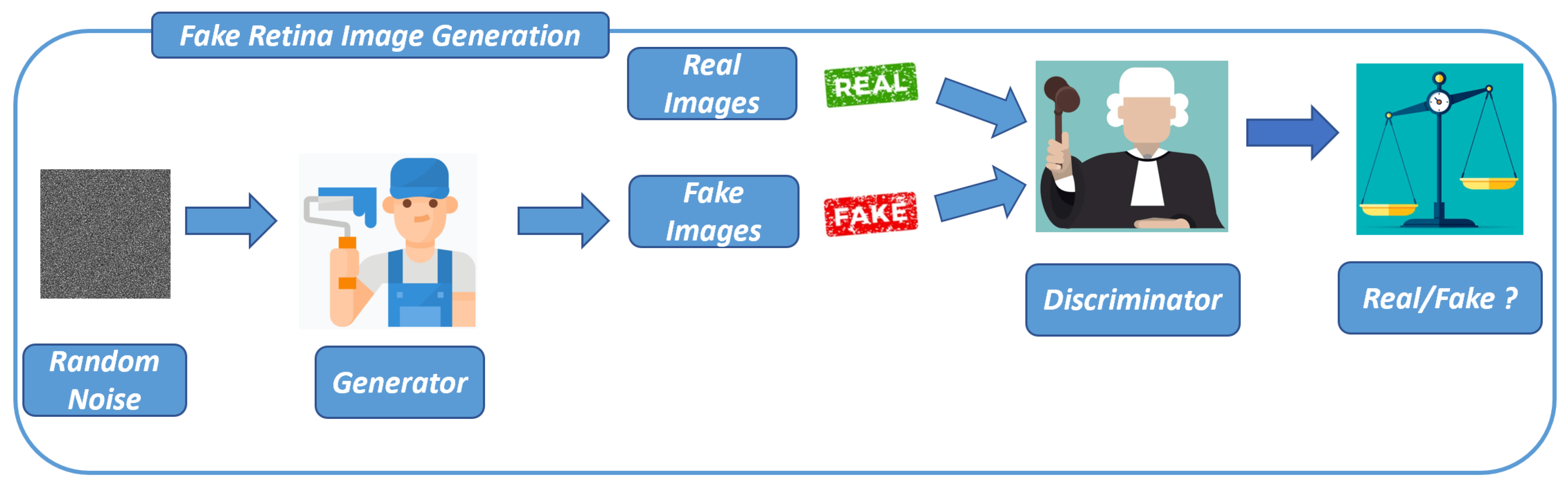
In a basic GAN architecture, two networks coexist, the generator model and the discriminator model. The term “adversarial” in GANs reflects their simultaneous training and competitive nature, resembling a zero-sum game like chess. The generator’s primary objective is to produce realistic images that can deceive the discriminator. In a simple GAN architecture for image synthesis, random noise is typically fed as input to the generator, which generates a corresponding image as output. On the other hand, the discriminator functions as a binary image classifier, responsible for determining the authenticity of an image by classifying it as real or fake.

To summarize, the basic GAN architecture involves the generator generating fake images, the discriminator classifying both real and fake images, and their performances being assessed separately.

Unlike most deep learning models that optimize towards minimizing a cost function (e.g., image classification), GANs operate differently. The generator and discriminator each have their own cost functions with opposing objectives. The generator aims to deceive the discriminator by generating fake images that resemble real ones, while the discriminator aims to accurately classify real and fake images.

During training, both the generator and discriminator improve their capabilities over time. The generator becomes more adept at producing images that closely resemble the training data, while the discriminator becomes more skilled at distinguishing between real and fake images.

Training GANs involve finding an equilibrium in the game, where the generator generates data that closely approximates the training data, and the discriminator can no longer differentiate between fake and real images.

A well-performing GAN model should exhibit high-quality images, such as non-blurry images resembling the training data, and diversity, meaning it should generate a wide range of images that capture the distribution of the training dataset.

Several noteworthy GAN variants have emerged, setting the stage for future advancements in the field. One prominent example is the DCGAN, which was the first GAN to integrate convolutional neural networks (CNNs) into its architecture. DCGAN has become one of the most widely adopted GAN models. Hence, in this paper, we employ the DCGAN framework for image generation.

3. The Method

We present the method we designed to (i) generate images related to the retina and (ii) discriminate these fake images from images obtained from real-world retina images.

The first step of the proposed method is the design and the adoption of the DCGAN to generate fake images related to the retina: this step is shown in Figure 1.

In every GAN, at least one generator (Generator in Figure 1) and one discriminator (Discriminator in Figure 1) are present. As the generator and discriminator engage in a competitive process, the generator enhances its capacity to generate images that closely align with the distribution of the training data, utilizing feedback received from the discriminator.

Thus, training a GAN is a crucial process that involves two neural networks, a generator (Generator in Figure 1) and a discriminator (Discriminator in Figure 1), competing against each other to improve their performance. In the following we provide an overview of the GAN training process:

1.

Initialization: Initially, the generator and discriminator networks are initialized with random weights.

2.

Objective: The objective of the generator is to create synthetic data that is indistinguishable from real data, while the discriminator’s objective is to correctly classify real data as real and generated data as fake.

3.

Training Loop:

(a)

Generator Training (Generator in Figure 1):

• The generator takes random noise as input and generates synthetic data.
• This generated data is mixed with real data (if available) to form a training batch.
• The output of the generator output is passed through the discriminator and the loss is calculated based on how well the discriminator was fooled (i.e., how well the generated data is classified as real).
• The weights of the generator are updated using gradient descent to minimize this loss, effectively improving its ability to generate more realistic data.

(b)

Discriminator Training (Discriminator in Figure 1):

• The discriminator takes both real and generated data as input and classifies them as real or fake.
• The loss for the discriminator is calculated based on how accurately it classifies real and generated data.
• The discriminator’s weights are updated to minimize this loss, making it better at distinguishing between real and generated data.

4.

Adversarial Training: The key idea in GANs is the adversarial training process, where the generator and discriminator iteratively improve their performance by competing against each other. As the training progresses, the generator becomes better at generating realistic data and the discriminator becomes better at distinguishing real from fake data.

5.

Convergence: Training continues for a set number of epochs or until a convergence criterion is met. Convergence occurs when the generator creates data that is so realistic that the discriminator cannot reliably distinguish it from real data.

6.

Evaluation: After training, the generator can be used to produce synthetic data and the discriminator can be used to assess the authenticity of data samples.

The DCGAN architecture introduced the incorporation of CNNs in both the discriminator and generator components.

DCGAN offers a set of architectural guidelines that aim to improve the stability of the training process [14]:

1.

Replace pooling layers with strided convolutions in the discriminator and fractional-strided convolutions in the generator;

2.

Incorporate batch normalization (batchnorm) in both the generator and discriminator;

3.

Avoid fully connected hidden layers in deeper architectures;

4.

Apply ReLU activation for all generator layers, except the output layer which employs Tanh activation;

5.

Employ LeakyReLU activation in all discriminator layers.

Strided convolutions refer to convolutional layers with a stride of 2, which are utilized in the discriminator for downsampling. On the other hand, fractional-strided convolutions, or Conv2DTranspose layers, employ a stride of 2 for upsampling in the generator.

In the context of DCGAN, batch normalization (batchnorm) is leveraged in both the generator and discriminator to enhance the stability of GAN training. Batchnorm normalizes the input layer by adjusting it to have a mean of zero and a variance of one. Typically, it is applied after the hidden layer and before the activation layer.

The DCGAN architecture commonly employs four activation functions: sigmoid, tanh, ReLU, and LeakyReLU.

Sigmoid function is utilized in the final layer of the DCGAN discriminator since it performs binary classification, producing an output of 0 (indicating fake) or 1 (indicating real).

Tanh function is similar to sigmoid but scales the output to the range [−1, 1], making it suitable for the generator’s last layer. Consequently, input data for training should be preprocessed to fit within the range of [−1, 1].

ReLU (rectified linear activation) returns 0 for negative input values and the input value for non-negative inputs. In the DCGAN generator, ReLU is used for all layers except the output layer, which employs tanh.

LeakyReLU is an extension of ReLU that introduces a small negative slope (controlled by a constant alpha) for negative input values. The recommended value for the slope (alpha) in DCGAN is 0.2. LeakyReLU activation is used in all layers of the discriminator, except for the last layer.

The training process involves simultaneous training of both the generator and discriminator networks.

The initial step involves data preparation for training the DCGAN. Since the generator model is not intended for a classification task, there is no need to split the dataset into training, validation, and testing sets. The generator requires input images in the format (60,000, 28, 28), indicating that there are 60,000 grayscale training images with dimensions of 28 × 28. The loaded data already has the shape (60,000, 28, 28) as it is grayscale.

To ensure compatibility with the generator’s final layer activation using tanh, we normalize the input images to the range of [−1, 1].

The primary objective of the generator is to generate realistic images and deceive the discriminator into perceiving them as real.

The generator takes random noise as input and generates an image that closely resembles the training images. Given that we are generating grayscale images of size 28 × 28, the model architecture needs to ensure that the generator’s output has a shape of 28 × 28 × 1.

To accomplish this, the generator performs the following operations:

1.

Convert the 1D random noise (latent vector) to a 3D shape using the Reshape layer.

2.

Upsample the noise iteratively using Keras.

3.

Match the Conv2DTranspose layer (also known as fractional-strided convolution in the paper) to the desired output image size. In our case, we aim to generate grayscale images with a shape of 28 × 28 × 1.

The generator comprises several key layers that serve as its building blocks:

1.

Dense (fully connected) layer: used primarily for reshaping and flattening the noise vector.

2.

Conv2DTranspose: employed for upsampling the image during the generation process.

3.

BatchNormalization: applied to stabilize the training process. It is positioned after the convolutional layer and before the activation function.

In the generator, ReLU activation is utilized for all layers, except the output layer, which employs tanh activation.

We developed a function for building the generator model architecture, for which a model summary is shown in

Table 1. Model generator.

#	Layer (Type)	Output Shape	Param #
1	dense (Dense)	(None, 12,544)	1,266,944
2	batch_normalization (BatchNormalization)	(None, 12,544)	50,176
3	re_lu (ReLU)	(None, 12,544)	0
4	reshape (Reshape)	(None, 7, 7, 256)	0
5	conv2d_transpose (Conv2DTranspose)	(None, 14, 14, 128)	819,328
6	batch_normalization_1 (BatchNormalization)	(None, 14, 14, 128)	512
7	re_lu_1 (ReLU)	(None, 14, 14, 128)	0
8	conv2d_transpose_1 (Conv2DTranspose)	(None, 28, 28, 64)	204,864
9	batch_normalization_2 (BatchNormalization)	(None, 28, 28, 64)	256
10	re_lu_2 (ReLU)	(None, 28, 28, 64)	0
11	conv2d (Conv2D)	(None, 28, 28, 1)	1601

.

For constructing the generator model, we utilized the Keras Sequential API. The initial step involved creating a Dense layer to reshape the input into a 3D format, with the input shape specified in this layer.

Following that, we added BatchNormalization and ReLU layers to the generator model. Subsequently, we reshaped the preceding layer from 1D to 3D and performed two upsampling operations using Conv2DTranspose layers with a stride of 2. This progression allowed us to increase the size from 7 × 7 to 14 × 14 and ultimately to 28 × 28.

After each Conv2DTranspose layer, we incorporated a BatchNormalization layer, followed by a ReLU layer.

Lastly, we included a Conv2D layer with a tanh activation function as the output layer.

The generator model comprises a total of 2,343,681 parameters, out of which 2,318,209 parameters are trainable, while the remaining 25,472 parameters are non-trainable.

Next, we will delve into the implementation of the discriminator model.

The discriminator functions as a binary classifier that discerns whether an image is real or fake. Its primary aim is to accurately classify the provided images. However, there are a few notable differences between a discriminator and a conventional classifier:

In the discriminator, we employ the LeakyReLU activation function. The discriminator encounters two categories of input images: real images sourced from the training dataset, labeled as 1, and fake images generated by the generator, labeled as 0.

It is worth noting that the discriminator network is usually designed to be smaller or simpler than the generator. This is because the discriminator has a relatively easier task compared to the generator. In fact, if the discriminator becomes too strong, it can impede the progress of the generator.

Table 2. Model discriminator.

#	Layer (Type)	Output Shape	Param #
1	conv2d_1 (Conv2D)	(None, 14, 14, 64)	1664
2	batch_normalization_3 (BatchNormalization)	(None, 14, 14, 64)	256
3	leaky_re_lu (LeakyReLU)	(None, 14, 14, 64)	0
4	conv2d_2 (Conv2D)	(None, 7, 7, 128)	204,928
5	batch_normalization_4 (BatchNormalization)	(None, 7, 7, 128)	512
6	leaky_re_lu_1 (LeakyReLU)	(None, 7, 7, 128)	0
7	flatten (Flatten)	(None, 6272)	0
8	dropout (Dropout)	(None, 6272)	0
9	dense_1 (Dense)	(None, 1)	6273

shows the model summary related to the discriminator model.

To create the discriminator model, we define a function that takes input consisting of either real images from the training dataset or fake images generated by the generator. These images have dimensions of 28 × 28 × 1, which are passed as arguments (width, height, and depth) to the function.

In constructing the discriminator model, we employ Conv2D, BatchNormalization, and LeakyReLU layers twice for downsampling. Then, we utilize the Flatten layer and apply dropout. Finally, in the last layer, we use the sigmoid activation function to produce a single value for binary classification.

The discriminator model comprises a total of 213,633 parameters, out of which 213,249 parameters are trainable, while 384 parameters are non-trainable.

The computation of loss plays a crucial role in training both the generator and discriminator models in DCGAN or any GAN architecture.

Specifically, for the considered DCGAN, we employ the modified minimax loss, utilizing the binary cross-entropy (BCE) loss function.

There are two separate losses that we need to calculate: one for the discriminator and another for the generator.

In terms of the discriminator loss, since the discriminator receives two groups of images (real and fake), we compute the loss for each group separately and then combine them to obtain the overall discriminator loss:

$$TotalDloss=loss\_from\_real\_images+loss\_from\_fake\_images$$

With regard to the generator loss, rather than training G to minimize $log(1-D(G\left(z\right))$, i.e., the probability that D classifies fake images as fake, we consider training G with the aim of maximizing $logD\left(G\right(z\left)\right)$, i.e., the probability that D incorrectly classifies the fake images as real: for this we exploit the modified minimax loss.

For both the generator and discriminator models, we utilize the Adam optimizer with a learning rate of 0.0002. As mentioned previously, we employ the binary cross-entropy loss function for both the discriminator and generator.

The training process involves training the models for a total of 50 epochs.

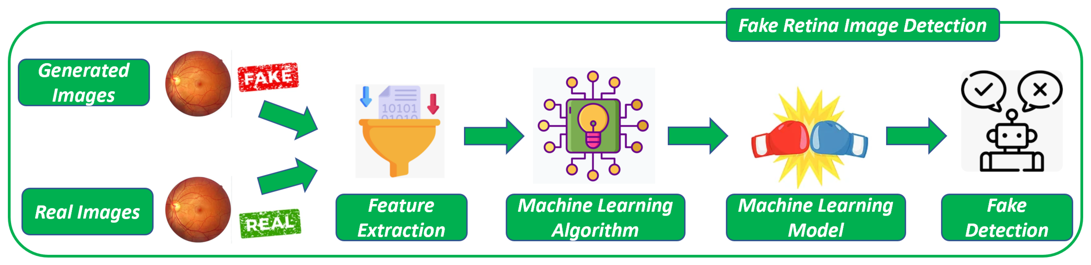
Once the images are generated with the DCGAN, the last step of the proposed method, shown in Figure 2, is devoted to building models aimed at discriminating between real and fake retina images.

In the proposed method, as depicted in Figure 2, the second step involves building a model to distinguish between generated and real images. To accomplish this, two datasets are required. The first dataset comprises real-world retina images, while the second dataset consists of images generated by the DGCAN (depicted in Figure 2). The real images utilized in the first step of the proposed method are the same as those used here.

From these two sets of images (i.e., Generated Images and Real Images in Figure 2), a set of numeric features is extracted (i.e., Feature Extraction in Figure 2). Specifically, the paper experiments with the Simple Color Histogram Filter [15] for this purpose. This filter calculates the histogram representing the pixel frequencies from each image. As a result, this filter extracts 64 numeric features from each image.

After obtaining the feature set from both the generated and real images, these features are used as inputs for a supervised machine learning algorithm (i.e., Machine Learning Algorithm in Figure 2). The goal is to construct a model that can determine whether an image is associated with a fake (generated) or a real application.

By training the machine learning algorithm with the extracted features, it learns patterns and relationships between the features and the authenticity of the images. This enables the model to classify new images as either fake or real based on the learned patterns (i.e., Machine Learning Model in Figure 2). The algorithm’s training involves providing it with labeled examples of images and their corresponding classification (fake or real), allowing it to learn the decision boundaries between the two classes. Once trained, the model can be used to predict the authenticity of unseen images (i.e., Fake Detection in Figure 2).

If the classifiers demonstrate optimal performance, there should be a noticeable distinction between the generated and original images. In contrast, if the machine learning models are unable to differentiate between the generated and original images, this suggests that the generated images closely resemble the originals.

To investigate the progression of image generation throughout the various stages of GAN training, a model is built for each epoch. This allows for an understanding of whether the generated images become progressively more similar to the original images. In order to ensure the validity of the conclusions drawn, the experimental analysis employs four different machine learning algorithms. Consequently, a total of 200 models (50 epochs multiplied by 4 algorithms) are considered for evaluation.

4. Experimental Analysis

We present and discuss the results of the experimental analysis we performed.

The goal of this experiment is to determine whether GANs can pose a threat to deep learning-based retina image classification. To achieve this, we exploited a DCGAN to generate a series of synthetic retina images. They then trained multiple classifiers to discern between real-world retina images and artificially generated ones.

Thus, we investigate whether the classifiers could accurately differentiate between real and fake retina images. Since the DCGAN generates a new dataset of retina images with each training epoch, the performance of the classifiers was tracked over time. The objective was to assess whether the classifiers’ ability to distinguish between real-world and synthetic images would decrease as the training progressed and the generated images presumably became more similar to real retina images.

By monitoring the performance of the classifiers, we determine whether the classifiers were successful in correctly identifying real images and distinguishing them from synthetic ones. If the classifiers’ performance declined as the training epochs increased, it would indicate that the classifiers struggled to differentiate between real and fake retina images.

Overall, the experiment aimed to evaluate the potential threat posed by GANs to deep learning-based retina image classification by examining the classifiers’ ability to discern between real-world and artificially generated images as the GAN training progressed.

For experimental purposes, we exploit the RetinaMNIST dataset, freely available for research purposes https://medmnist.com/ (accessed on 18 August 2023), based on the DeepDRiD challenge, which provides a dataset of 1600 retina fundus images. The retina images are related to the five-level grading of diabetic retinopathy severity. The source images are center-cropped and resized to 3 × 28 × 28 [16,17].

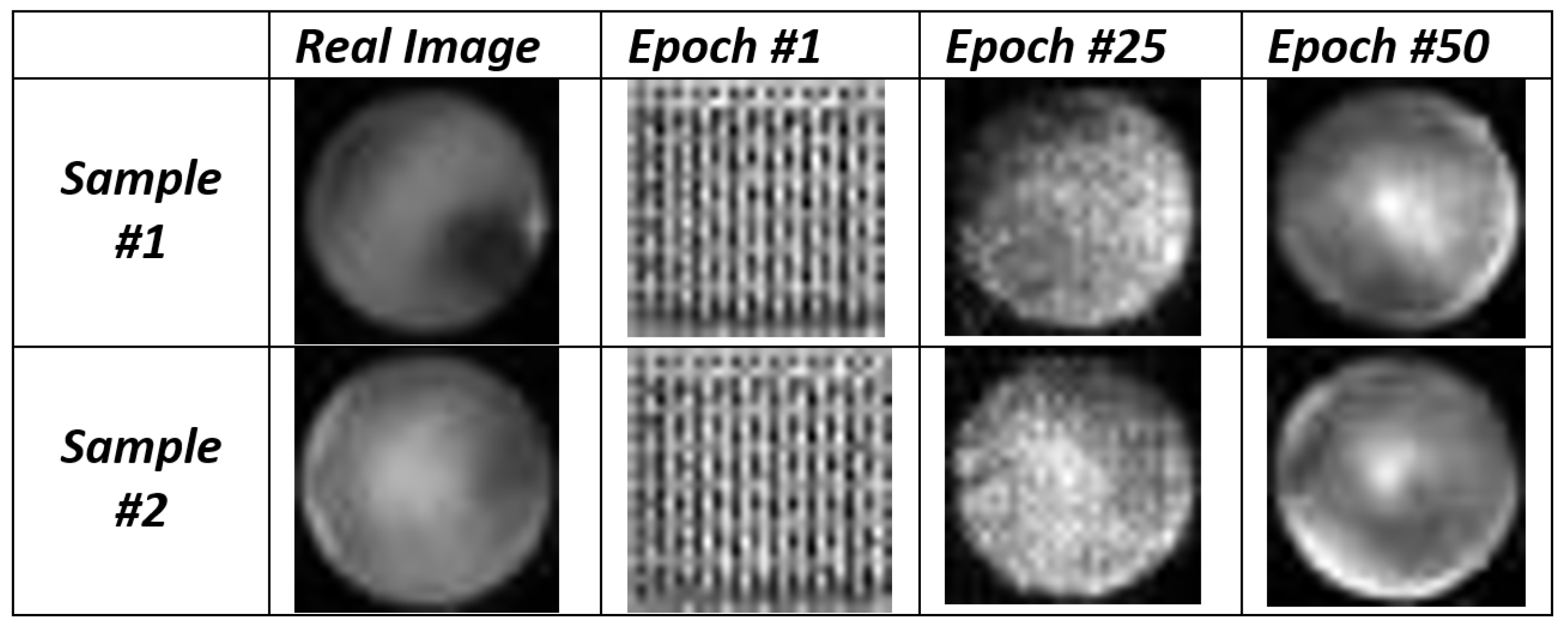
In the experimental analysis, the DCGAN was trained for a total of 50 epochs. Each epoch took around 25 seconds to complete, utilizing the computational power of an NVIDIA T4 Tensor Core GPU. For each epoch, the DCGAN generated a batch of 1000 synthetic retina images.

In Figure 3 we show a set of images generated by the DCGAN at different epochs and the original input images used for the DCGAN for the fake retina image generation.

From the images shown in Figure 3 we consider two different (original) input images (i.e., Real Image Sample #1 and Real Image Sample #2): we can note that at epoch #1 the DCGAN generated only noise (and this is an expected behavior), while in the 25th epoch the fake images obtained from both sample #1 and #2 are closer to the real images. In the last, the 50th one, we can note that the images are quite similar to the real ones.

To assess the performance of the classifiers, several metrics were considered. These metrics include Precision, Recall, and F-Measure.

Precision is a measure of the accuracy of the classifier in identifying true positives among the samples it predicted as positive. It represents the ratio of true positives to the sum of true positives and false positives. A higher precision indicates a lower rate of false positives. It is computed as follows:

$$\mathit{Precision}=\frac{tp}{tp+fp}$$

where tp indicates the number of true positives and fp indicates the number of false positives.

Recall, also known as sensitivity or true positive rate, measures the ability of the classifier to identify all positive instances correctly. It is calculated as the ratio of true positives to the sum of true positives and false negatives. A higher recall indicates a lower rate of false negatives. It is computed as follows:

$$\mathit{Recall}=\frac{tp}{tp+fn}$$

where fn indicates the number of false negatives.

F-Measure, or F1 score, is the harmonic mean of precision and recall. It provides a balanced measure that takes into account both precision and recall. The F-Measure considers the trade-off between precision and recall, giving equal importance to both metrics. It is computed as the weighted average of precision and recall, where the weights are determined by their relative importance. It is computed as follows

$$\mathit{F}-\mathit{Measure}=2*\frac{Precision*Recall}{Precision+Recall}$$

By evaluating the Precision, Recall, and F-Measure of the classifiers, the authors aimed to gain insights into their effectiveness in distinguishing between real and fake retina images generated by the DCGAN. These metrics provide a comprehensive understanding of the classifiers’ performance in terms of accuracy, true positive rate, and the balance between precision and recall.

Four different widespread supervised machine learning classifiers are exploited with the aim of enforcing conclusion validity: J48 [18], SVM [19], Random Forest [20], and Bayes [21].

In the experiment, the authors built a separate model for each algorithm and for each epoch, resulting in a total of 200 different models. Specifically, there were four algorithms considered and each algorithm had a model built for every epoch.

To construct each model, a combination of real-world application images and synthetic images generated by the DCGAN for a specific epoch was used. This means that, for each epoch, the researchers had a dataset that included both real retina images from real-world applications and synthetic retina images generated by the DCGAN.

By creating multiple models for each algorithm and epoch, the researchers aimed to analyze the performance and effectiveness of the classifiers in distinguishing between real and fake retina images at different stages of the training process. This approach allows any changes in the classifier performance to be observed as the DCGAN generated images that were presumably becoming more similar to real retina images over the course of the training epochs.

Below, we explain how we built and evaluated the machine learning models designed to differentiate between real and fake retina images.

Relating to the model learning, we consider T as a set of labels {(M, l)}, where each M is the label that is associated with an l∈ { real, fake}.

For the M model, we build a numeric vector of features F $\in R_y$, where y represents the number of features exploited in the learning phase ($y=64$; as a matter of fact, this is the number of numeric features obtained, from each image, by applying the Simple Color Histogram Filter).

In more detail, with respect to the training phase, k-fold cross-validation is exploited. We explain this process: the instances of the dataset are split in a random way into a set denoted as k.

In order to test the effectiveness of both the models we propose, the procedure explained below is considered:

1.

Generation of a set for the training, i.e., T⊂D;

2.

Generation of an evaluation set $T^{\prime }=D÷$ T;

3.

Execution of the model training T;

4.

Application of the model previously generated to each element of the $T^{\prime }$ set.

To mitigate the risk of overfitting, we employed cross-validation in their evaluation process. Cross-validation ensures that all samples in the dataset are evaluated during the testing phase. Below we explain how we accomplished cross-validation:

1.

Data Splitting: The entire dataset, consisting of real and fake retina images, was divided into k equal-sized parts or folds. The value of k determines the number of subsets the dataset is divided into.

2.

Training and Validation Iteration: During each iteration of the cross-validation process, one of the folds was designated as the validation set, while the remaining k − 1 folds were used as the training set. This process was repeated k times, with each fold taking turns as the validation set.

3.

Model Training and Evaluation: For each iteration, a separate model was trained using the training set. The performance of the model was then evaluated using the validation set. The evaluation metrics, such as Precision, Recall, and F-Measure, were calculated based on the model’s predictions on the validation set.

4.

Performance Aggregation: The performance of the model was assessed across all k iterations. The individual performance scores from each iteration were aggregated to obtain an overall estimate of the model’s performance. Typically, this aggregation is performed by calculating the mean of the performance scores across the iterations.

In this study, the researchers chose a value of k = 10, which means the dataset was divided into 10 equal parts and the iteration was repeated 10 times. Each fold served as the validation set once, while the remaining nine folds were used for training the model. The final performance metrics were calculated as the average of the metrics obtained from the 10 iterations.

This approach helps to mitigate overfitting and provides a more realistic evaluation of the classifiers’ performance in distinguishing between real and fake retina images.

In

Table 3. Experimental analysis results for epochs 0, 25, and 49.

Epoch	Algorithm	Precision	Recall	F-Measure
0	J48	1	1	1
	SVM	0.990	0.989	0.989
	RandomForest	1	1	1
	Bayes	0.999	0.999	0.999
25	J48	0.970	0.970	0.970
	SVM	0.956	0.954	0.954
	RandomForest	0.974	0.974	0.974
	Bayes	0.958	0.957	0.957
49	J48	0.972	0.971	0.971
	SVM	0.939	0.936	0.936
	RandomForest	0.974	0.973	0.973
	Bayes	0.956	0.955	0.955

we show the experimental analysis results: for the reason of space we report the results related to three epochs: the first one (i.e., 0 in the column Epoch), the middle one (i.e., 25 in the column Epoch), and the final one (i.e., 49 in the column Epoch), with the aim of understanding the general trend.

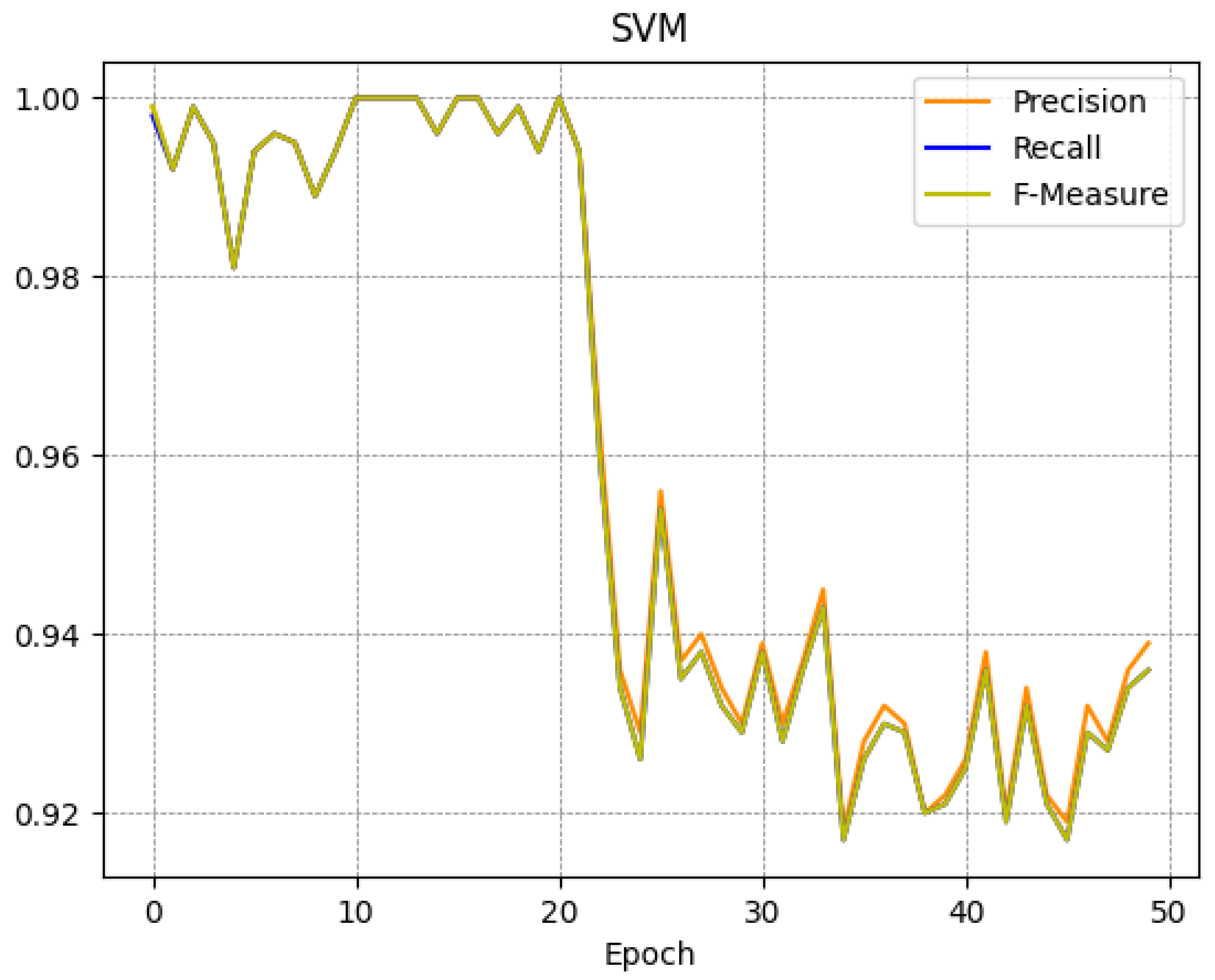
From Table 3 it emerges that when the number of epochs is increasing the metrics, i.e., Precision, Recall, and F-Measure, suffer a decrease: for instance at epoch 0 the SVM F-Measure is equal to 0.989, at epoch 25 it is equal to 0.954, and at epoch 49 it is equal to 0.936. We also note that this trend is not reflected in the J48 model: as a matter of fact, at epoch 0 the J48 model F-Measure is equal to 1, at epoch 25 it is equal to 0.970, and at epoch 49 it is equal to 0.971. So we can say that from epoch 25 to epoch 49 the J48 performances remain substantially unchanged.

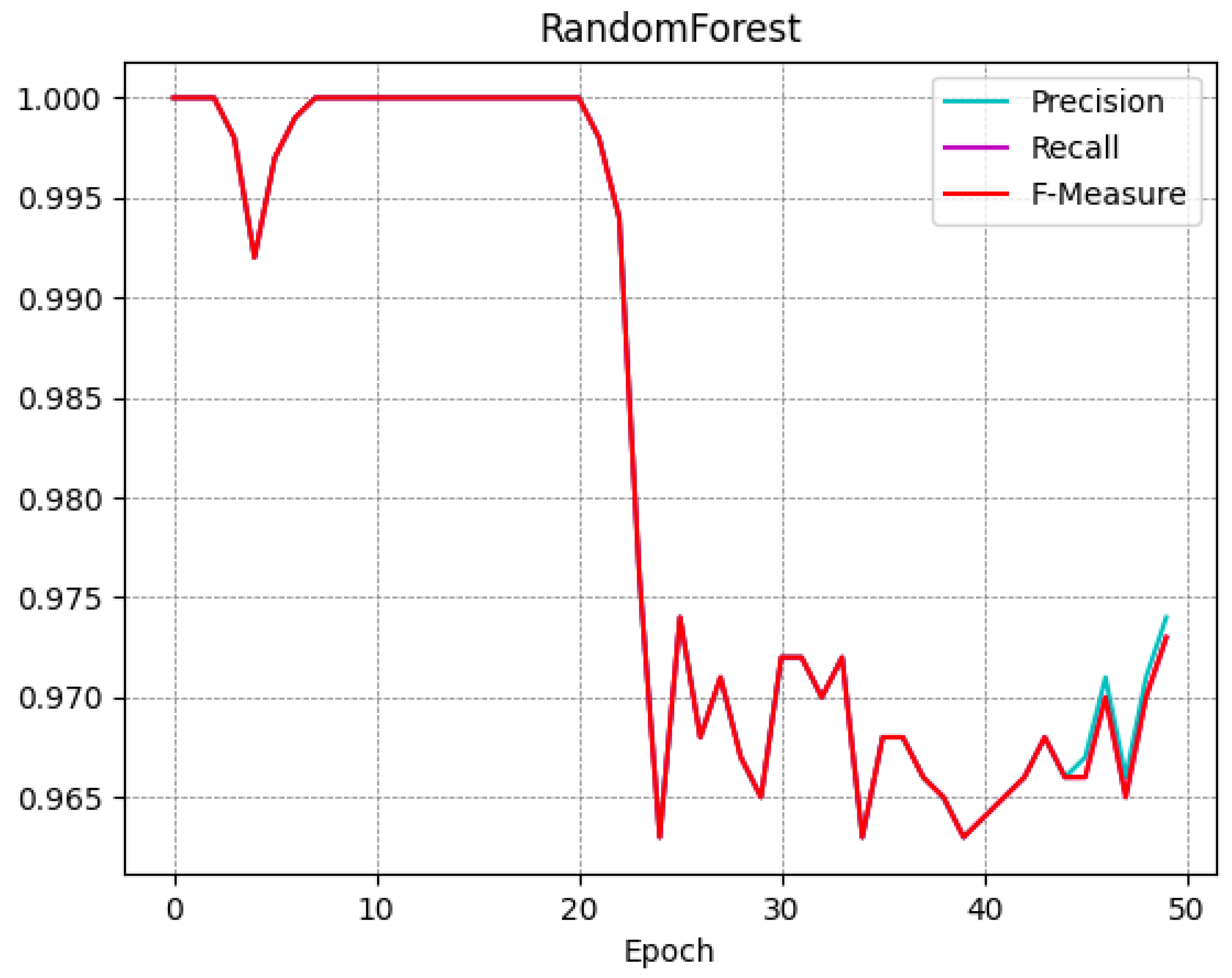
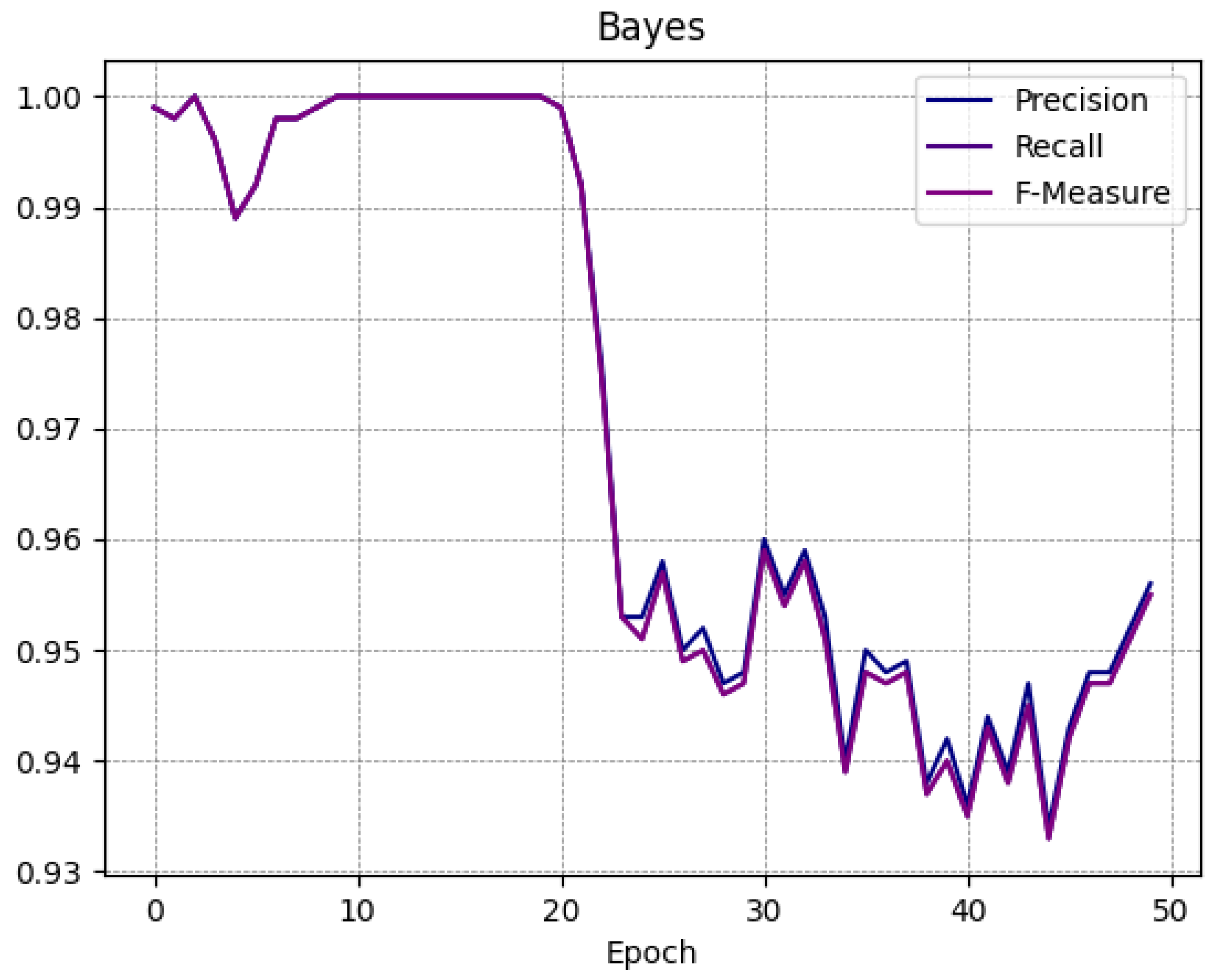
A trend similar to the one obtained from the SVM classifier is shown in the RandomForest model, in fact; at epoch 0 the F-Measure is equal to 1, at epoch 25 it is equal to 0.974, and at epoch 49 it is equal to 0.973. A similar consideration can be made with respect to the Bayes model, with an F-Measure equal to 0.999 at epoch 0, an F-Measure of 0.957 at the 25-th epoch, and an F-Measure equal to 0.955 with regard to epoch 49.

This decreasing trend obtained when the epoch number is increasing is something that is expected, considering that the GAN learns to build better (fake) retina images at each epoch: but, as we noticed in the results shown in Table 3, the performance decay is minimal but still present. Thus, the series of retinal images fail to be distinguished correctly by the classifier.

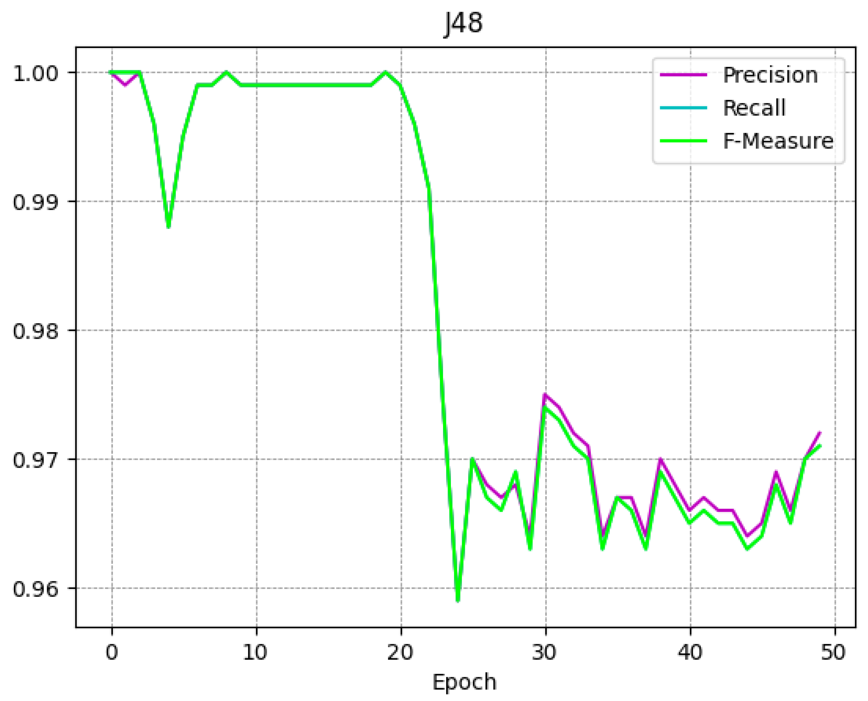
To better understand the trend of the classifiers during the several epochs, in Figure 4, Figure 5, Figure 6 and Figure 7 we show the plot of the F-Measure trend for the 50 epochs, for the J48 model shown in Figure 4, the SVM model shown in Figure 5, the RandomForest one shown in Figure 6, and the Bayes model shown in Figure 7.

All supervised learning models exhibit a very similar trend as shown in Figure 4, Figure 5, Figure 6 and Figure 7: this confirms that the trend obtained is general and not specific to a single model. Note that the decay (of the Precision, Recall, and F-Measure metrics) occurs approximately after 20 epochs.

We, therefore, note that the performance decay is present even if minimally; therefore, if, on the one hand, the classifier continues to obtain good performances even with images obtained after 50 epochs, on the other hand, it is still possible to note that some of the false images are indistinguishable from real ones for classifiers.

In addition to the machine learning classifier experiments, in

Table 4. Experimental analysis results for 49th epoch with deep learning models.

Algorithm	Precision	Recall	F-Measure
LeNet	0.480	0.480	0.480
AlexNet	0.985	0.985	0.985
CustomCNN	0.519	0.519	0.519
MobileNet	0.973	0.973	0.973

we present the experimental results we obtained with four deep learning models. In particular, the following models are considered: LeNet [22], AlexNet [23], CustomCNN [24,25], and MobileNet [26]. In the deep learning experiment, we consider the retinal images generated in the last epoch.

From the results shown in Table 4 it emerges that the results obtained with the machine learning models (shown in Table 3) are similar to the ones exhibited by deep learning models. In particular, the AlexNet and the MobileNet models show an F-Measure respectively equal to 0.985 and to 0.973, while the LetNet and the CustomCNN models obtained an F-Measure respectively equal to 0.480 and to 0.519.

In summary, the experimental analysis results suggest that, currently, GANs do not pose a significant threat because existing classifiers can effectively distinguish between real and fake images. However, we recall that a small percentage of images can still evade detection, which could potentially become a threat in the future, particularly in the context of biomedical image classification.

5. Discussion

As already mentioned in the introduction section, GANs have shown significant promise in a plethora of fields, including the biomedical context. However, similarly to any newly proposed method, GANs come with their own set of strengths and weaknesses when applied to biomedical applications. In this section, we discuss the strong points and the weaknesses of GAN adoption related to the biomedical context and we provide a table aimed at summarizing the state of the art in the adoption of GANs in the biomedical context with particular regard to the papers related to retinal images.

In the following we itemize the strong points related to GAN adoption in the biomedical context:

• Data Augmentation: GANs can generate synthetic data that closely resemble real biomedical data. This is particularly useful when the available dataset is small or lacks diversity. GAN-generated data can be used to augment the training data, leading to better model generalization.
• Image Synthesis: GANs excel at generating high-quality images. In the biomedical field, this can be used for tasks like generating medical images (e.g., MRI and CT scans) with different contrasts, resolutions, or pathologies. It can aid in medical image analysis and training image-based models.
• Drug Discovery: GANs can generate molecular structures with desired properties. They can be used for drug discovery by generating novel chemical structures that match specific criteria, potentially accelerating the drug development process.
• Data Privacy: GANs can generate synthetic data that preserve the statistical properties of the original data while ensuring privacy. This can help in sharing medical data without revealing sensitive patient information.
• Noise Reduction: GANs can be employed to denoise biomedical images, which is crucial for accurate medical diagnosis. They can help in improving the quality of noisy or low-resolution images.

Below we itemize the weaknesses related to GAN adoption in the biomedical context:

• Data Quality: GANs are highly sensitive to input data quality. If the initial dataset contains errors, biases, or inaccuracies, the generated data may inherit these issues, potentially leading to unreliable results.
• Mode Collapse: GANs can suffer from mode collapse, where the generator produces a limited variety of outputs, failing to capture the full diversity of the underlying data distribution. This can hinder the effectiveness of the model.
• Training Challenges: GANs can be challenging to train and require careful tuning of hyperparameters. Training instability, vanishing gradients, and mode dropping are common issues that can make training difficult.
• Ethical Concerns: In the biomedical field, generating synthetic medical images that are indistinguishable from real ones raises ethical concerns. There is a risk of inadvertently creating misleading or potentially harmful information.
• Interpretability: GANs are often considered "black box" models, making it challenging to interpret how they generate certain outputs. This lack of interpretability can be problematic in medical applications where understanding the decision-making process is crucial.
• Generalization: GAN-generated data might not perfectly mimic real-world data distribution, leading to potential challenges in generalizing the models to real-world scenarios. Careful validation and testing are required to ensure real-world applicability.

In summary, GANs offer valuable contributions in the biomedical context, particularly in data augmentation, image synthesis, and drug discovery. In

Table 5. The state-of-the-art comparison in the adoption of GAN in the biomedical context.

Authors	GAN Type	Contributions	F-Measure
Orlando et al. [27]	ACGAN	Developed a GAN for generating retinal images with lesionss	0.78
Schlegl et al. [28]	ACGAN	Introduced a conditional GAN for retinal image generation.	0.92
Fu et al. [29]	ACGAN	Used ACGAN to generate synthetic retinal images for augmentation.	0.88
Costa et al. [30]	ACGAN	Extended ACGAN for multi-modal retinal image synthesis.	0.89
Lahiri et al. [31]	ACGAN	Developed a GAN-based method for retinal vessel segmentation.	0.91
Tufail et al. [32]	DCGAN	Explored the use of GANs for generating retinal images.	0.75
Skandarani et al. [33]	StyleGAN	Utilized StyleGAN to generate high-resolution retinal images.	0.87
Sevastopolsky et al. [34]	ACGAN	Proposed a GAN approach for retinal image synthesis for glaucoma detection.	0.86
Khalid et al. [35]	ACGAN	Further advancements in conditional GANs for retinal image synthesis.	0.91
Bellemo et al. [36]	ACGAN	Explored the use of ACGANs for generating diabetic retinopathy images.	0.82
Our method	DCGAN	Assess the the potential impact of GANs on retinal image classification tasks.	0.973

we provide a table with a state-of-the-art comparison between different research papers combining GAN and biomedical images in terms of the kind of GAN exploited (i.e., GAN Type column), the contributions of the paper, and the obtained F-Measure.

As emerges from the comparison shown in Table 5 there are several research papers exploring the adoption of GAN in the biomedical context, for several purposes, for instance from the generation of retinal images with lesions proposed by Orland et al. [27] to the retinal image augmentation proposed by Fu and colleagues [29]. As mentioned in the introduction section, the main aim of the proposed method is to understand whether GAN can be considered to generate retinal images that are not distinguishable from the real ones and this represents the main contribution of this paper. The results of the experimental analysis demonstrated that every model attained an F-Measure surpassing 0.95, suggesting the effective identification of the majority of retinal images GAN generated. Nonetheless, it was also noted that certain retinal images were able to avoid detection by the classifiers designed for retinal fake image detection.

Furthermore, it is important to note that, while GANs offer significant advantages in biomedical image analysis, their use in critical medical applications requires thorough validation, and careful consideration of ethical and regulatory concerns. The quality of generated images and their clinical relevance must be rigorously assessed before deploying GAN-based solutions in real healthcare settings.

6. Conclusions and Future Work

Considering the realistic nature of images generated by GANs, there is a need to assess their potential threat to image recognition systems, particularly in the field of biomedical image classification. In this paper, we proposed a method to evaluate whether retinal images generated by a DCGAN can be distinguished from real images. We employed eight different supervised machine learning algorithms to build a model capable of distinguishing between real and fake retinal images. The experimental analysis revealed that all the models achieved an F-Measure greater than 0.95, indicating that most of the fake images were successfully recognized. However, we also observed that some retinal images managed to evade detection by the fake image classifiers. On one side, GANs can address limited dataset issues by generating synthetic data that resemble real biomedical data, aiding in training robust models, and they excel at creating high-quality medical images, aiding in medical image analysis, disease diagnosis, and treatment planning, but on the other they are sensitive to input data quality and may inherit errors or biases. It may be of interest to develop such a system in the real world as the generation of fake images could be used to poison a classifier, thus adding fake images to the training dataset. Therefore, to guarantee the quality of a dataset composed, for example, of images of the retina, such a system could be used in a machine learning pipeline to verify the veracity of the images present in the training dataset. As a matter of fact, the rapid expansion of machine learning’s presence in biomedical research frequently leads to an oversight regarding the reliability of these studies. In fact, machine learning has proven highly effective in various domains (with particular regard to the biomedical one), yet its success is vulnerable to malicious actions. Adversarial attacks, which involve manipulations intended to disrupt predictions, pose a substantial threat to the practical use of machine learning. These attacks encompass evasion attacks, which manipulate only test data, and poisoning attacks, in which the attacker introduces tainted test and/or training data. A comprehensive grasp of adversarial attacks and the development of appropriate defenses are essential for upholding the reliability of machine learning applications. We think that this is one of the most interesting aspects that can boost the proposed method in the real world. Obviously, we are aware that the results obtained could vary depending on the biomedical field analyzed, but also if the DCGAN were trained for a greater number of epochs or if a different type of GAN was used. For these reasons, among other future developments, we will evaluate the effectiveness of the proposed method using different types of GANs and different types of biomedical images acquired by different machines. As a matter of fact, in future research, we intend to explore other types of biomedical images and evaluate alternative GAN architectures such as conditional generative adversarial networks and cycle-consistent generative adversarial networks to compare their performance against the DCGAN used in this study.