Exploring Design Optimization of Self-Compacting Mortars with Response Surface Methodology

Abstract

The ever-evolving construction sector demands technological developments to provide consumers with products that meet stringent technical, environmental, and economic requirements. Self-compacting cementitious mixtures have garnered significance in the construction market due to their enhanced compaction, workability, fluidity, and mechanical properties. This study aimed to harness the potential of statistical response surface methodology (RSM) to optimize the fresh properties and strength development of self-compacting mortars. A self-compacting mortar repository was used to build meaningful and robust models describing D-Flow and T-Funnel results, as well as the compressive strength development after 24 h (CS24h) and 28 days (CS28d) of curing. The quantitative input factors considered were A (water/cement), B (superplasticizer/powder), C (water/powder), and D (sand/mortar), and the output variables were Y1 (D-Flow), Y2 (T-Funnel), Y3 (CS24h), and Y4 (CS28d). The results found adjusted response models, with significant R² values of 87.4% for the D-Flow, 93.3% for the T-Funnel, and 79.1% for the CS24h. However, for the CS28d model, a low R² of 39.9% was found. Variable A had the greatest influence on the response models. The best correlations found were between inputs A and C and outputs Y1 and Y2, as well as input factors A and D for responses Y3 and Y4. The resulting model was enhanced, thereby resulting in a global desirability of approximately 60%, which showcases the potential for the further refinement and optimization of RSM models applied to self-compacting mortars.

1. Introduction

Concrete is one of the main elements used in civil construction, due to its variability in use, which only intensifies with urban development. However, concrete production heavily relies on natural resource consumption, including the fundamental constituents for cement production and the extraction of coarse and fine aggregates, thereby causing deleterious environmental impacts [1,2].

Self-compacting concrete (SCC) was developed to improve concrete fluidity and self- consolidation properties, thus obviating the requirement for external compaction elements while also fostering enhanced mechanical properties [3,4,5,6]. When producing self-compacting cement-based products, it is recommended to reduce the proportion of coarse aggregates and to increase the amount of fine aggregates and cement to reduce the risk of segregation and increasing properties such as viscosity, void filling, and stability, in addition to mechanical properties [7]. However, such a mix design approach may be prone to cracking and shrinkage, in addition to increased production costs [5,8].

The use of mineral and chemical additives in SCC aims to increase durability and workability while reducing production costs [9,10]. Moreover, contemporary architecture demands slender structures of highly intricate and complex geometry, which increase the demand for innovative self-leveling mortars and concrete with a high strength development [10,11,12]. However, the design of high-strength cement-based materials with self-compacting attributes is challenges due to inherent contradictions in mixture design requirements. For instance, achieving a high early strength typically requires low water/binder ratios (w/b), which, conversely, reduce the mixture’s self-compacting ability. Therefore, traditional mixed design approaches may prove inadequate when addressing the demanding requirements of self-compacting mortars. Data-driven mixed design methodologies may offer a promising alternative method to gain valuable insights on how to enhance the fresh properties of self-compacting mortars while maximize their strength development. Design of experiments (DoE) is a statistical tool that has been used in the optimization of materials, and its advantages include correlating the investigated variables, finding an optimal response within an investigation region, reducing the number of required experimental trials, and even defining optimized models according to predefined parameters [13,14]. The response surface methodology (RSM) can be used to find relationships between input and output variables and to define the optimization criteria among variables [15,16,17,18].

In recent decades, investigations using statistical tools in concrete and mortar mix design have been intensified. Research has applied the RSM to maximize the replacement of cement or aggregates with—among others—pumice stone [1], foundry sand [18], plastic waste and silica fume [19], and hybrid steel fibers [20]. The authors developed high-significance models, thereby making it possible to optimize the performance of cementitious mixtures while reducing the use of prime raw materials. Other studies were undertaken with the primary objective of improving the environmental and economic performance of cementitious materials [21,22,23,24,25,26,27,28,29,30,31,32,33,34,35,36,37,38].

More recently, the use of statistical methodologies has gained attention in the realm of self-compacting cementitious materials. Its application extends to various domains, thus encompassing the assessments of rheological effects and mechanical properties, as well as the mitigation of early-stage cracking. Li et al. [39] employed regression models, utilizing central composite design (CCD), to examine the influence of four mixed design variables (fly ash content (FA), silica fume content (SF), sand–binder ratio (s/b), and water–binder ratio (w/b)) on the rheological and mechanical properties of concrete. The responses measured included mini slump flow, mini V-funnel results, and compressive strength after 28 days of curing. The authors applied multiresponse optimization to determine the optimal ranges for each compositional variable (FA: 10–20 wt%, SF: 6–10 wt%, s/b: 1.1–1.2, w/b: 0.35–0.36). Similarly, Safhi et al. [40] investigated the feasibility of using treated marine sediments as cement replacements in self-compacting mortars. The authors’ findings indicated that treated marine sediments led to reductions in the mechanical performance (the elastic modulus and compressive strength) while having no significant deleterious effects on the rheological properties. The authors prescribed a sediment-to-cement ratio ranging from 0.0703 to 0.3462 to maintain acceptable levels of mechanical performance loss while benefiting from the reduced environmental impact and production costs.

Conversely, Matos et al. [28] focused on addressing the early-stage cracking proclivity of self-compacting ternary white mortars. The authors found that quadratic models were suitable for adequately describing the mortar’s properties, and subsequent mix design optimization steps allowed for reductions in segregation (the T-Funnel time increased from 8.5 to 9.8 s) and yearly shrinkage (which reduced from 558 × 10⁻⁶ to 540 × 10⁻⁶) that significantly minimized the risk of cracking.

In a prior publication [41], the authors comprehensively characterized the performance of self-compacting mortars, which they made publicly available in a substantial dataset encompassing a wide array of rheological and mechanical properties.

The objective of the study herein is to advance the data analysis leveraging the statistical tool of RSM through a central composite design to define, adjust, and optimize models for high-performance self-compacting mortars a based upon the aforementioned experimental dataset.

2. Materials and Methods

The performance of self-compacting mortars was evaluated using published datasets, which were collected during the authors’ previous experimental studies [41].

The mortar specimens were produced using CEM I 42.5 R cement, limestone filler, normalized sand, and a polycarboxylate-based superplasticizer. The cement was purchased from Secil Portugal (Outão, Portugal) and was compliant with EN 197-1 specifications. Limestone filler with specific gravity of 2.68 g/cm³ was provided by Omya S.A under the commercial reference of Betocarb 10 HP—OU. Normalized sand compliant with EN 196-1 was used in all experiments, with a water absorption of 0.30% and specific gravity of 2.63 g/cm³. The selected superplasticizer (ViscoCrete^®-20 HE, from SIKA, Vila Nova de Gaia, Portugal) was characterized by a density of 1.08 g/cm³ and a solid content of 40%.

The dataset includes a total of thirty formulations of self-compacting mortars with four quantitative input variables. A central composite design was defined using Design–Expert software (Stat-Ease, Inc., Minneapolis, MN 55413-2561, USA—Design–Expert^® Software, version 13.0.9.0 64-bit; Serial Number 0964-0841-3719-3394) consisting of a factorial design of four factors in two levels (2⁴) representing 8 axial and 6 central realizations. The four input variables analyzed included the following—A: water-to-cement ratio (w/c); B: superplasticizer-to-powder (CEM I 42.5 R + limestone filler) ratio (Sp/p); C: water-to-powder (CEM I 42.5 R + limestone filler) ratio (w/p); and D: sand-to-mortar ratio (s/m). All ratios refer to volumetric relations. The evaluation levels were −∞, −1, 0, +1, and +∞, with ∞ being equal to 2.

Table 1. Equivalence of coded and real values (reproduced from [41]).

Levels	A: w/c	B: Sp/p	C: w/p	D: s/m
−2	0.78741	0.02069	0.46929	0.42240
−1	0.84110	0.02210	0.50129	0.45120
0	0.89478	0.02351	0.53328	0.48000
+1	0.94847	0.02492	0.56528	0.50880
+2	1.00216	0.02633	0.59728	0.53760

shows the relation between coded points and real values.

Workability and strength development were evaluated as outputs. Four response variables were defined and examined, namely, these included the following: Y1: D-Flow results (in mm); Y2: T-Funnel (in seconds); and compressive strength measured after 1 and 28 days of curing (Y3 and Y4, respectively, both expressed in MPa). The D-Flow and T-Funnel testing were conducted following EFNARC specifications and guidelines for self-compacting concrete, whereas compressive strength was determined as per EN 196-1. The detailed description of the testing protocols can be found elsewhere [41]. For compressive strength measurements, a minimum of four specimens was tested with respect to formulation and curing age. The average strength values were considered representative, and only those values are reported here. All experiments have been conducted in randomized order.

Table 2. Coded input variables and results for response factors (adapted from [41]).

Std	Run	Coded Values				Results
		A	B	C	D	Y1	Y2	Y3	Y4
1	11	−1	−1	−1	−1	325	22	62.7	115.8
2	29	1	−1	−1	−1	341	18	55.7	108.0
3	21	−1	1	−1	−1	325	21	62.7	112.1
4	26	1	1	−1	−1	359	15	57.7	114.6
5	9	−1	−1	1	−1	361	16	60.6	114.5
6	1	1	−1	1	−1	377	12	53.4	109.0
7	27	−1	1	1	−1	368	13	58.2	115.8
8	23	1	1	1	−1	370	13	55.6	105.1
9	22	−1	−1	−1	1	229	108	61.4	104.1
10	18	1	−1	−1	1	318	31	55.5	106.4
11	6	−1	1	−1	1	309	162	62.9	111.2
12	30	1	1	−1	1	308	30	53.9	101.8
13	2	−1	−1	1	1	304	29	62.0	112.5
14	5	1	−1	1	1	344	19	54.6	106.9
15	17	−1	1	1	1	328	24	61.7	111.4
16	8	1	1	1	1	342	18	56.9	112.2
17	25	−2	0	0	0	270	45	62.9	103.9
18	20	2	0	0	0	345	16	51.3	106.0
19	10	0	−2	0	0	329	21	58.4	117.7
20	24	0	2	0	0	349	17	56.7	115.4
21	15	0	0	−2	0	306	40	60.4	113.5
22	16	0	0	2	0	358	13	57.4	114.0
23	14	0	0	0	−2	370	12	57.5	114.6
24	19	0	0	0	2	282	52	58.8	110.0
25	4	0	0	0	0	342	18	60.2	108.2
26	7	0	0	0	0	339	21	58.7	107.2
27	13	0	0	0	0	332	19	58.5	111.7
28	12	0	0	0	0	348	17	56.1	113.8
29	3	0	0	0	0	338	19	59.2	117.7
30	28	0	0	0	0	338	24	61.7	*

*—Not possible to be measured.

shows the coded input values (A–D) and the average result of each individual response (Y1–Y4).

3. Results

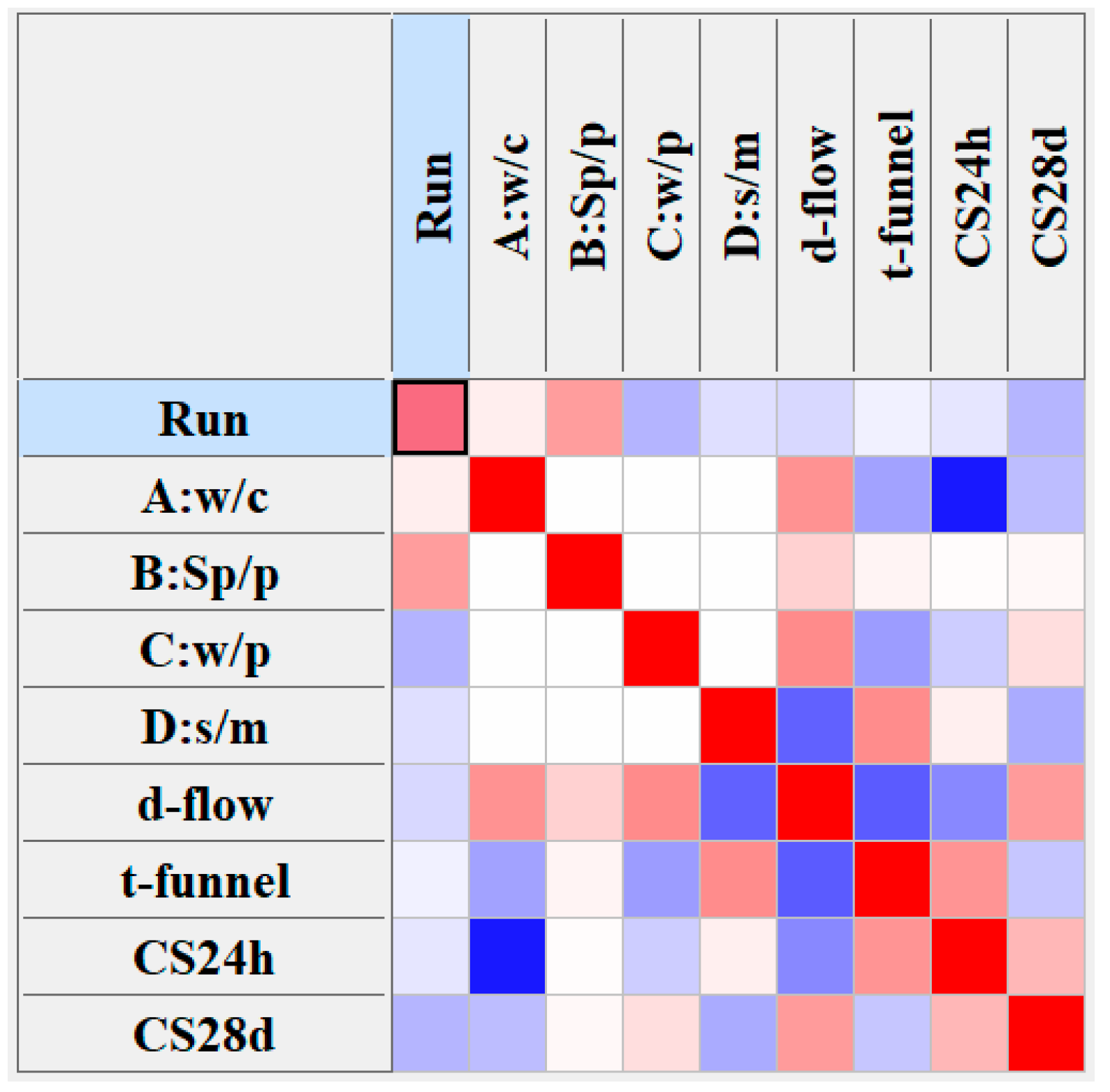
3.1. Preliminary Data Analysis

Table 3. Responses of 30 self-compacting concrete mixes.

Levels	Y1	Y2	Y3	Y4
	D-Flow (mm)	T-Funnel (s)	CS24h * (MPa)	CS28d * (MPa)
Minimum	229	12	51.3	101.8
Maximum	377	162	62.9	117.7
Mean	332	29	58.4	110.9
Std. Dev.	32	31	3.1	4.4
CV (%)	10	106	5.3	4.0

* CS24h and CS28d stand for compressive strength after 1 and 28 days of curing, respectively.

shows the minimum, maximum, mean, standard deviation, and coefficient of variation values of the investigated response variables. The collected data was homogenous and presented low standard deviation and coefficients of variation that indicate concentration around the mean values. However, this pattern was not observed in the flow results obtained through the T-Funnel test, which displayed a more dispersed distribution, which was reflected through a higher coefficient of variability (CV = 106%).

Figure 1 shows the heatmap of the correlations between the input and output variables. The degree of interaction between the variables is shown according to color. Positive correlations are indicated in shades of red, whereas negative correlations are indicated in shades of blue. Strong correlations can be observed between A and Y3 (−0.878), Y1 and Y2 (0.642), and D and Y2 (−0.618). However, a significant number of moderate positive correlations, ranging between ±0.363 and ±0.465, primarily existed and comprised Y1 and Y2 variables. It is crucial to assess whether these correlations have an impact on the behavior of the self-compacting mortars, and therefore should be reflected in response models.

3.2. Fresh Properties of Self-Compacting Mortars

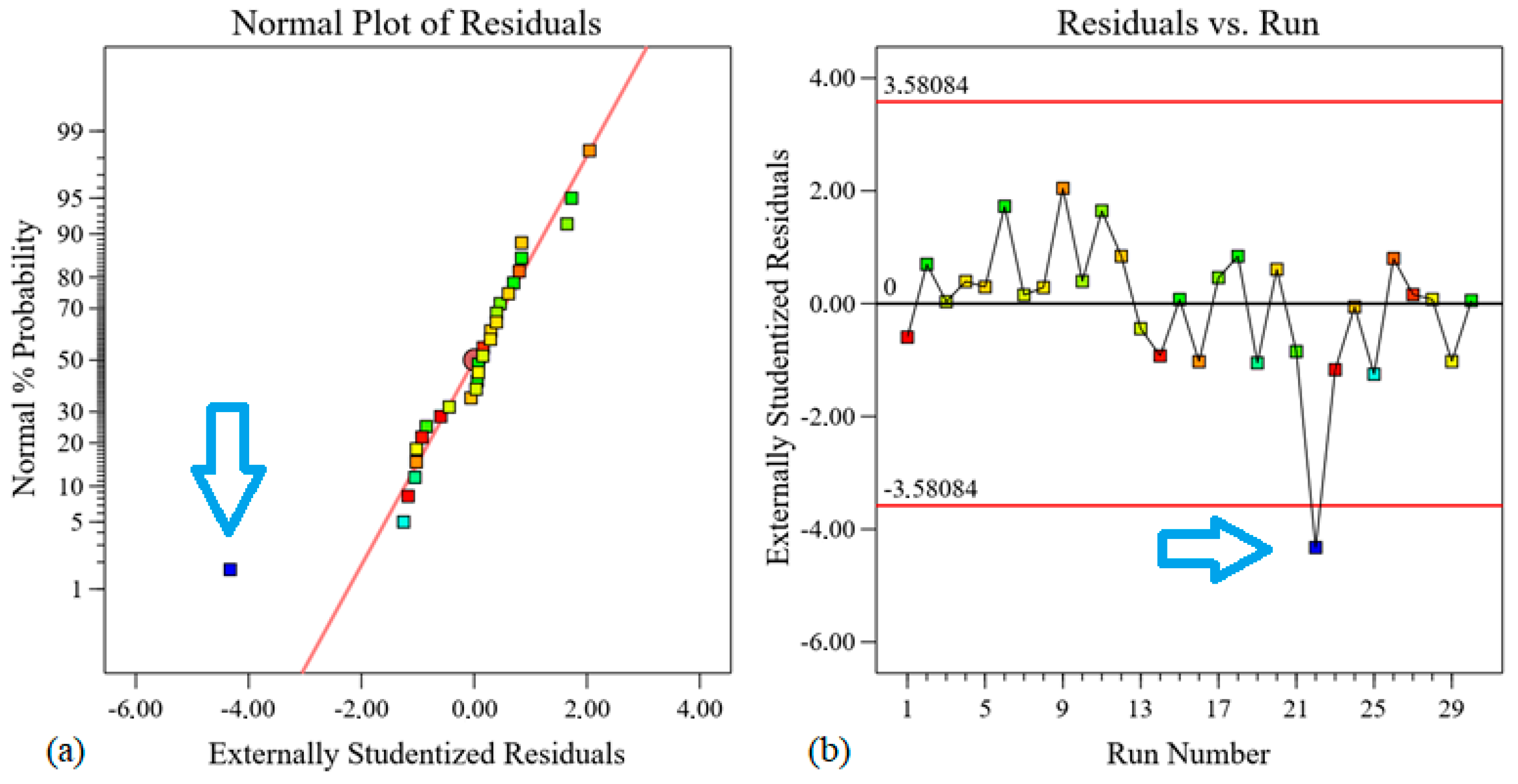
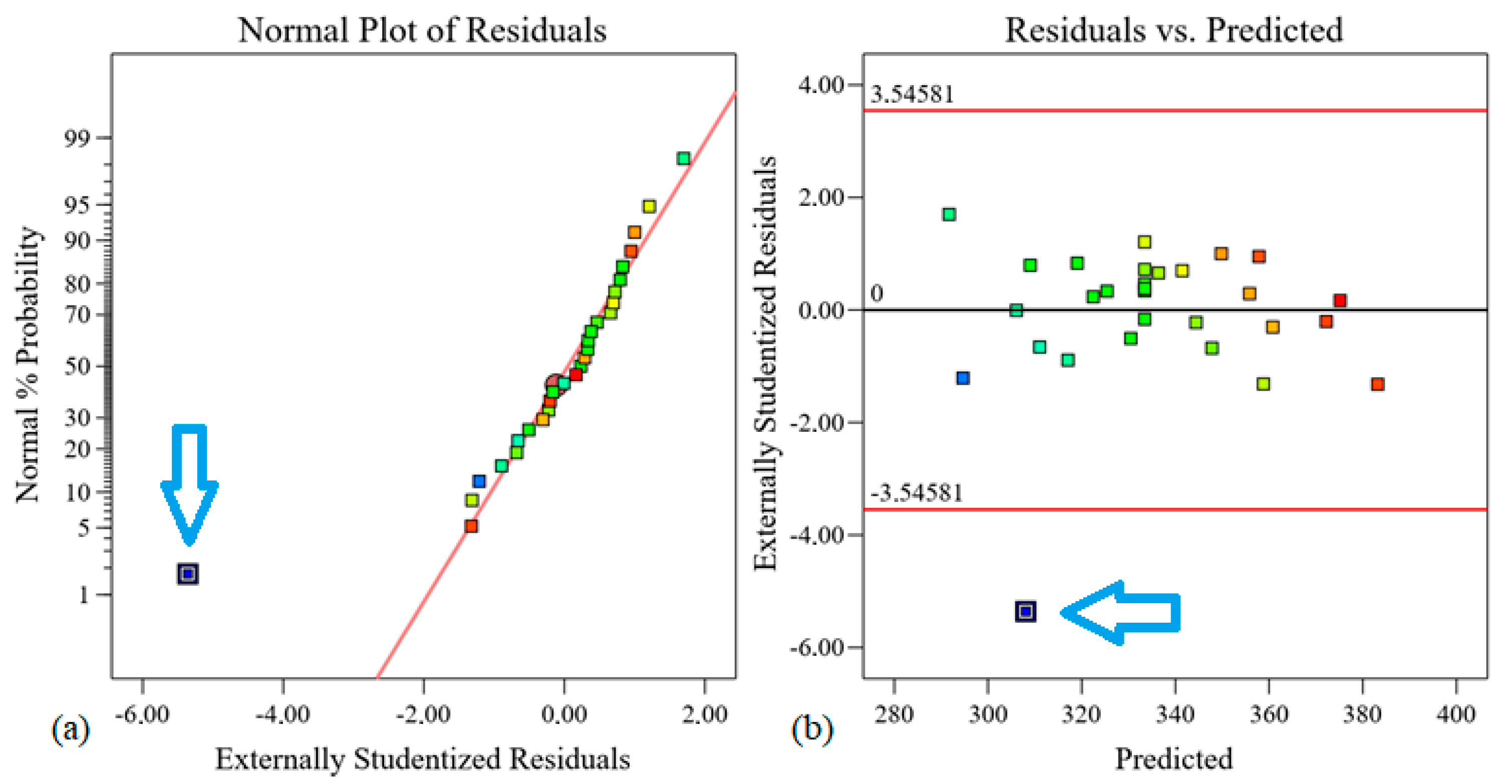
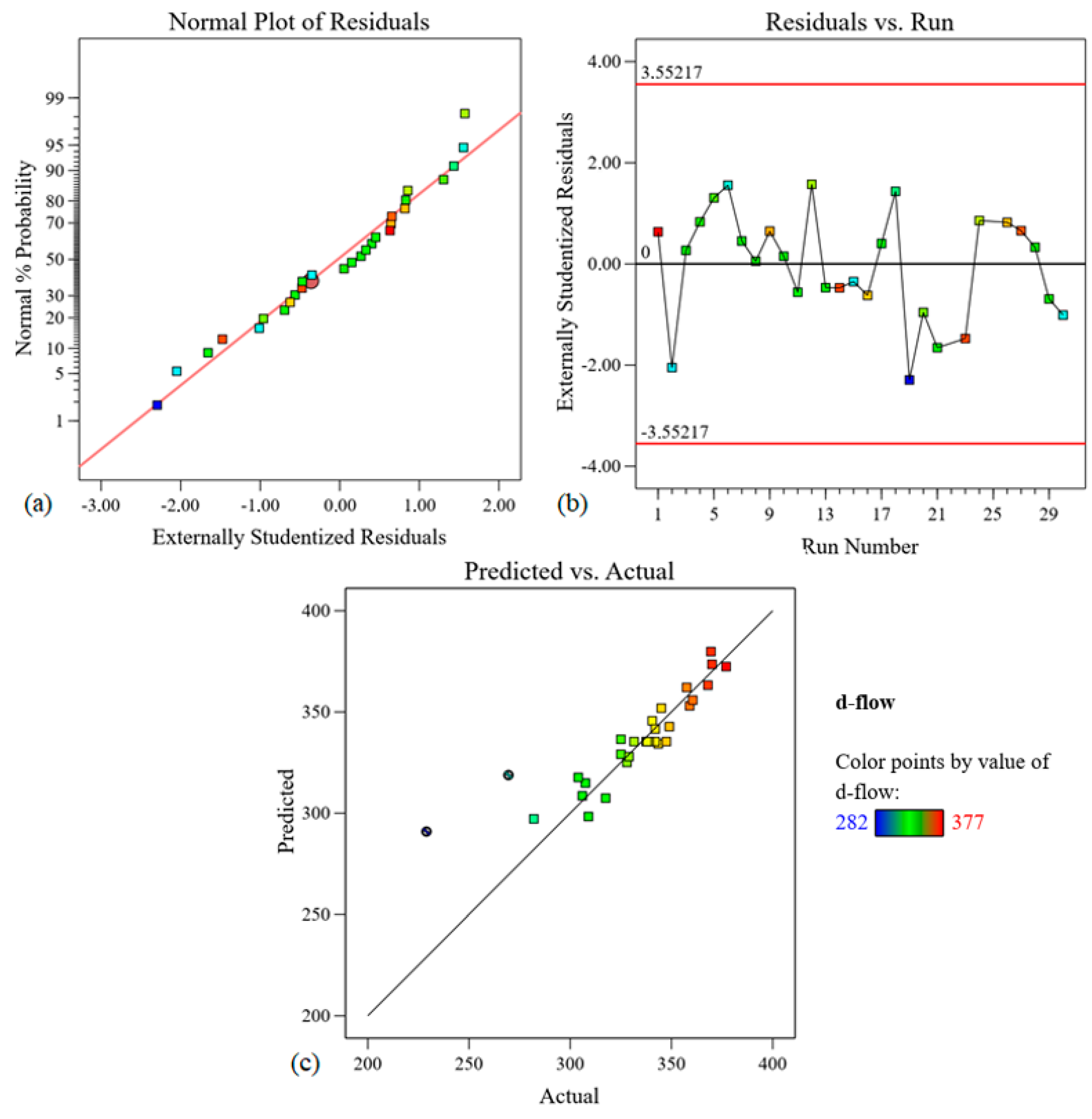
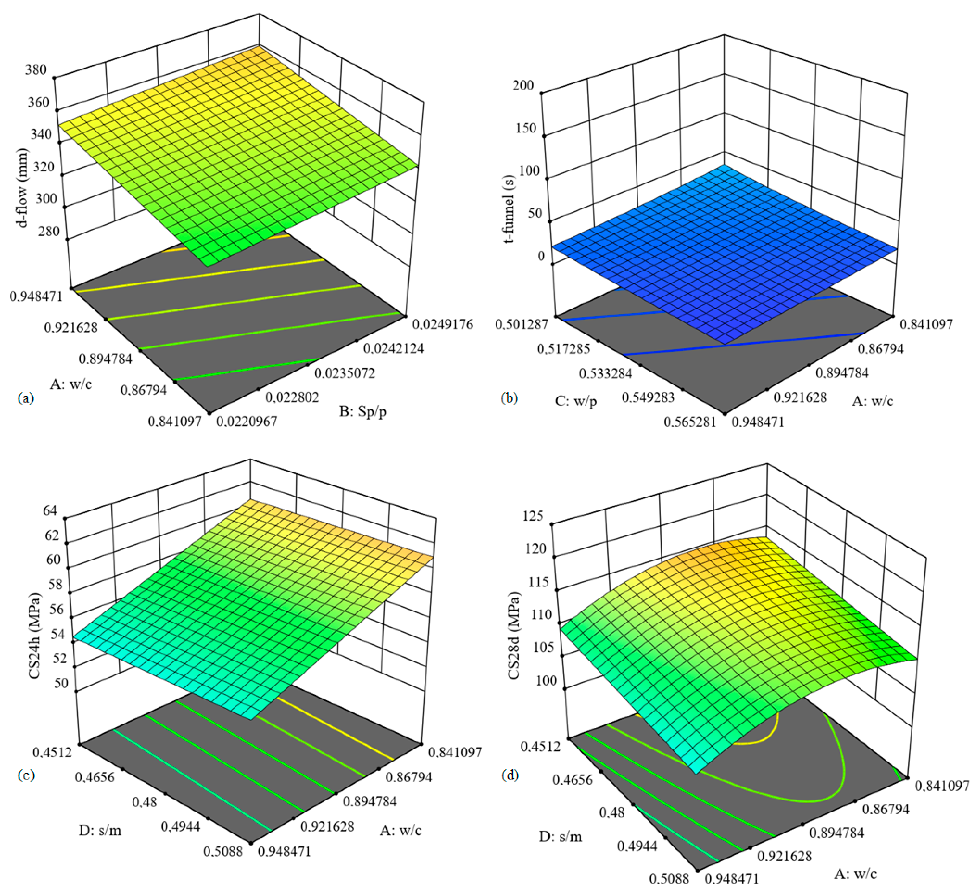
Regression Model for D-Flow

The regression analysis has shown that the quadratic models exhibited a superior fit. Notably, they presented an adjusted R² of 84.2% and a predicted R² of 76.0%, both of which had discrepancy values of less than 20%. However, the analysis of variance (ANOVA) revealed a “Lack of fit F-value” of 7.04, along with an associated p-value of 0.02. Consequently, there was only a 2% calculated likelihood that the lack of fit F-value could be attributed to random noise; it was more likely a result of the overall model’s shortcomings. Hence, these findings highlighted the necessity for refinement of the polynomial model to ensure its soundness and validity. Figure 2 shows the normal probability of the residuals (a) and the residuals versus the run plot (b) as part of the data diagnostic analysis. These graphical representations provide valuable insights into the behavior of the residuals from the regression model. Notably, an evident outlier was observed in data point Std 9, Run 22, which exhibited significant deviations in the Y1 results compared to the remaining realizations. Similar outlier patterns were also noticed in relation to the Y2 output variable. In addition, Cook’s distance, DFFITS, and DFBETAS, which are commonly used measures to assess the influence of individual data points on regression models (not shown here for the sake of brevity), indicate that this particular realization significantly departed from the majority of data points, thereby demonstrating its status as an outlier. The exact cause for such behavior remains unknown; however, it is most likely attributed to experimental variability during the preparation or testing of the mortar specimens. As a consequence, to ensure the robustness of the analysis, this outlier data point was excluded from the dataset, and a subsequent run was conducted that considered the revised dataset.

After excluding the outlier data point, a second run was conducted that demonstrated that the linear regression models presented better fitting than the quadratic models.

The analysis of variance (ANOVA) yielded adjusted R² values of 78.6% and a predicted R² of 71.3%, which can be considered to be fairly reasonable results, with differences being smaller than 20%. Despite its significance, the linear model F-value (6.16) indicated a suboptimal fitting. Therefore, the data diagnostic analysis was repeated to ensure the reliability of the analysis and identify any remaining outliers.

Figure 3 displays that the Std 17, Run 25 data point exhibited an outlier profile similar to the previously excluded Std 9 data point. The Cook’s distance, DFFITS, and DFBETAS plots further confirmed the classification of Std 17, Run 25 as an outlier, although they are not shown here for the sake of brevity.

Analogously to the previous case, the outlier was also excluded, and a new analysis was conducted, wherein the linear model yielded satisfactory results. The key performance indicators of the model are presented in

Table 4. Fitting results for D-Flow fitted models.

Source	Sum of Squares	Mean Square	F-Value	p-Value
Model	12,633.5	3158.4	47.7	<0.0001
A-w/c	1266.9	1266.9	19.1	0.0002
B-Sp/p	314.3	314.3	4.8	0.0399
C-w/p	4079.9	4079.9	61.6	<0.0001
D-s/m	8303.5	8303.5	125.4	<0.0001
Residual	1523.0	66.2
Lack of Fit	1382.7	76.8	2.74	0.135
Pure Error	140.4	28.1
Cor Total	14,156.5	-

. The model proved to be statistically significant, as evidenced by a p-value of less than 0.0001 and an F-value of 47.70. Furthermore, terms A, B, C, and D were also significant, with values lower than 0.1. Particularly noteworthy are the superior outcomes observed for terms C and D, which corroborates the model’s nonreduction. The F-value was 2.74, thus implying that the associated error was not statistically significant. The probability of such an error being attributed to noise surpassed 13.45%, thereby confirming the model’s suitability for use.

The model’s statistical fitting demonstrated enhanced performance, with the predicted R² value reaching 83.15% and the adjusted R² reaching 87.37%. The adequate precision value was found to be 24.03 (>>4.0), thus further indicating a robust relationship between the signal and noise and the model discrimination. In addition, the standard deviation was reduced to 8.14, which was accompanied by a coefficient of variation of 2.41%. Therefore, the model effectively described the design space, and

Table 5. Coefficients of coded factors—D-Flow.

Factor	Intercept	A—w/c	B—Sp/p	C—w/p	D—s/m
Coefficient Estimate	335.32	8.27	3.71	13.38	−19.09
Standard Error	1.56	1.89	1.70	1.70	1.70
95% CI Low	332.10	4.36	0.19	9.85	−22.62
95% CI High	338.54	12.19	7.24	16.91	−15.56
VIF	-	1.01	1.01	1.01	1.01

shows the estimated coefficients that were obtained. These coefficients were derived from fits around the overall average of all the runs in an orthogonal design, and the variance inflation factor (VIF) exceeding 1.0 demonstrates that the factors A, B, C, and D were found to be multicollinear.

Figure 4 shows the normal probability of the residuals (a), the Residuals versus Run plot (b), and the Predicted versus Actual plot (c). The normal probability of the residuals exhibited a linear trend, thereby suggesting a favorable model fit. In addition, a desirable random dispersion pattern is observed, with all data points falling within the specified limits (±3.55) (Figure 4b). A strong correlation can be observed between the predicted and actual values, with the data points exhibiting a clear tendency to align in a preferential direction. Also located are the excluded points (Std 9, Run 15 and Std 17, Run 25) in the RSM (Figure 4c).

3.3. Regression Model for T-Funnel

The best response model for the T-Funnel was the 2FI (two-factor interaction), which obtained a predicted R² of 15.58% and an adjusted R² of 69.72%, which are values that are considered significant. The percentage difference between the predicted and adjusted values was 54.14% (a value well above 20%), which is not recommended, as the errors are expected to be significant.

The model, despite being considered significant in its best response, had a significant lack of fit, which is not ideal, as there are high chances of errors. An inverse transform was recommended by the Box–Cox plot diagnostic to improve the overall model fit. A lambda (λ) equal to −1 was considered within the 95% confidence interval, with its limits ranging between of −1.55 and −0.93.

After applying the inverse transform (λ= −1), the linear model yielded the most significant fit (

Table 6. Fitting results for T-Funnel linear model (inverse).

Source	Sum of Squares	Mean Square	F-Value	p-Value
Model	0.0117	0.0029	101.78	<0.0001
A-w/c	0.0019	0.0019	65.19	<0.0001
B-Sp/p	0.0001	0.0001	4.70	0.0398
C-w/p	0.0037	0.0037	128.64	<0.0001
D-s/m	0.0060	0.0060	208.57	<0.0001
Residual	0.0007	0.0000
Lack of Fit	0.0005	0.0000	0.7718	0.6949
Pure Error	0.0002	0.0000
Cor Total	0.0124	-

). The F-value of 101.78 indicates that there is only a 0.01% probability of such a result being attributed to random noise. Furthermore, the terms A, B, C, and D were statistically significant, as their p-values were less than 0.05. The lack of fit was not significant, thus further demonstrating the well-fitting property of the model. The F-value for the lack of fit was 0.77, and there was a 69.49% chance that the lack of fit could be attributed to noise. The predicted R² was 91.79%, while the adjusted R² was slightly higher at 93.29% (ANOVA analysis). These results show a strong correlation between the predicted and actual values. The low standard deviation of 0.0054 reinforces the model’s significance. A precision value of 36.02 further supports the model’s efficacy.

Table 7. Coefficients in terms of coded factors—D-Flow.

Factor	Intercept	A–w/c	B–Sp/p	C–w/p	D–s/m
Coefficient Estimate	0.0499	0.0088	0.0024	0.0124	−0.0158
Standard Error	0.0010	0.0011	0.0011	0.0011	0.0011
95% CI Low	0.0479	0.0066	0.0001	0.0102	−0.0181
95% CI High	0.0519	0.0111	0.0046	0.0147	−0.0136
VIF		1.00	1.00	1.00	1.00

shows the estimated coefficients for the T-Funnel linear model. All of the input variables exhibited a standard error of 0.0011, thereby indicating the precision of the estimates. Moreover, the variance inflation factor (VIF) has been calculated to be 1.00, thus corroborating the orthogonality of the factors studied here.

The residual normal probability plot in Figure 5a reveals that the data points were closely aligned with the straight line, despite adopting an S-shaped pattern, which indicates a satisfactory distribution of the residuals. The Residuals versus Run plot demonstrates random dispersion, thus lacking any discernible trend. Notably, the scattered data points fell well within the specified limits of ±3.54047. Figure 5c shows lambda (λ) values of −1, which lie within the confidence interval (CI) of −1.55 to −0.93. Figure 5d illustrates the relationship between the predicted and actual points, thereby providing an intuitive visual insight into the model’s good predictive performance and accuracy. Complementary analyses, such as the Residuals versus Predicted, Residuals versus Water/Cement, Cook’s Distance, Leverage, DFFITS, and DFBETAS, yielded results within the established limits in good agreement with such observations.

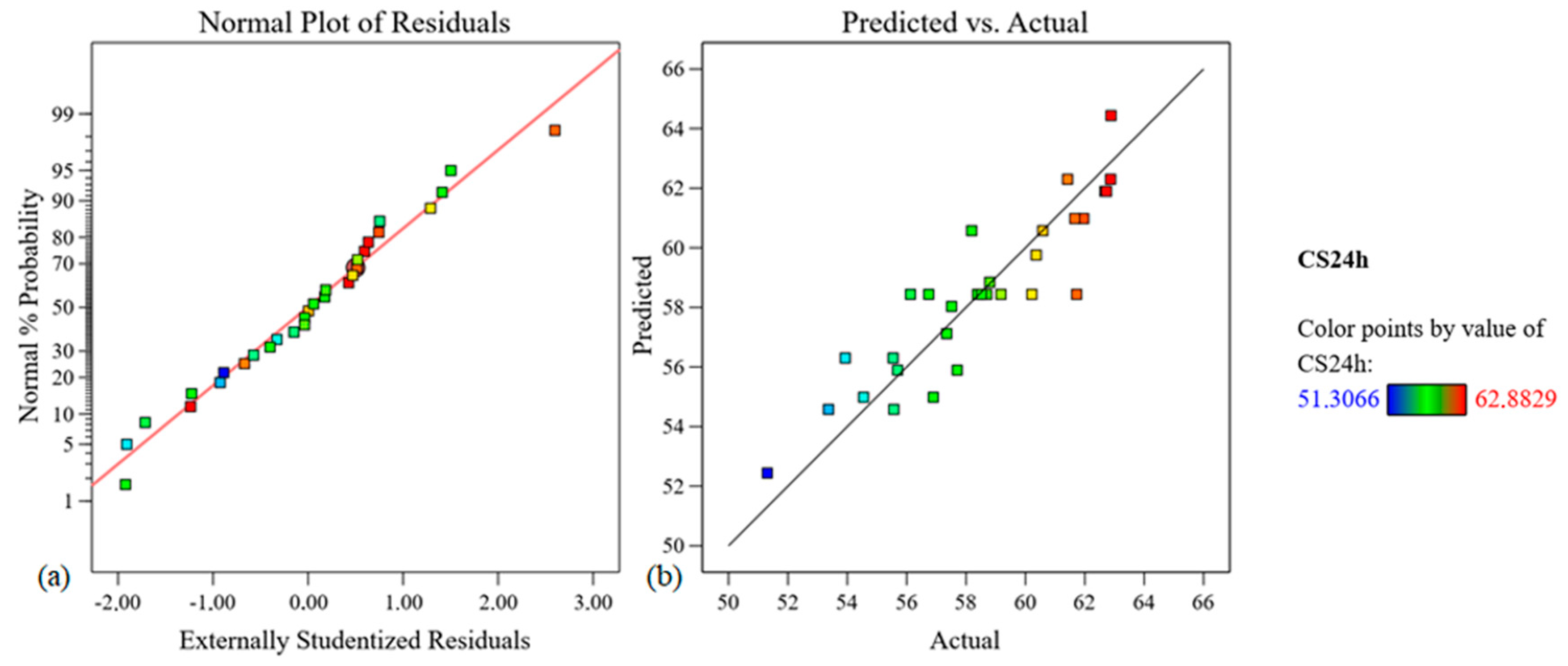
3.4. Regression Model for 24-Hour Compressive Strength

For the 24 h compressive strength (CS24h) measurements, regression analysis was performed in order to define the polynomial model. The reduced linear model (removing factor B) was the one that best presented satisfactory results. The B term was removed from the model due to its considerably high p-value (0.9491), which aimed at enhancing the model performance. Due to the linear nature of the model, the removal of the B term did not influence the other terms.

Table 8. Fitting results for compressive strength results after 24 h of curing.

Source	Sum of Squares	Mean Square	F-Value	p-Value
Model	227.36	75.79	37.54	<0.0001
A—w/c	215.95	215.95	106.96	<0.0001
C—w/p	10.42	10.42	5.16	0.0316
D—s/m	0.9928	0.9928	0.4917	0.4894
Residual	52.49	2.02
Lack of Fit	35.04	1.67	0.4778	0.8934
Pure Error	17.46	3.49
Cor Total	279.86	-

shows the model’s F-value of 37.54 and p-values below 0.05, thereby providing evidence of the model’s statistical significance after removing term B. The terms A and C were also deemed to be statistically significant, as was supported by their high sum of squares values and p-value less than 0.05 (0.001 for A and 0.0351 for C). The F-value was calculated to be 0.4778, thereby surpassing the significance level of 0.05 and indicating that the lack of fit was not statistically significant concerning pure error. The possibility of a misfit F-value occurring due to noise only stood at approximately 89.34%.

The results of the regression model revealed a predicted R² value of 0.7607, which agreed well with an adjusted R² value of 0.7908. The difference between the predicted and adjusted R² values being less than 20% indicates the model’s statistical significance. Moreover, the model demonstrated an adequate precision of 23.1254, thereby showcasing its ability to accurately describe the modeled data space. The standard deviation of the regression model was calculated to be 1.42, with a coefficient of variation (CV) of 2.43%.

Table 9. Coefficients in terms of coded factors—compressive strength after 24 h of curing.

Factor	Intercept	A—w/c	C—w/p	D—s/m
Coefficient Estimate	58.44	−3.00	−0.6589	0.2034
Standard Error	0.2594	0.290	0.2900	0.2900
95% CI Low	57.91	−3.60	−1.26	−0.3928
95% CI High	58.97	−2.40	−0.0628	0.7996
VIF	-	1	1	1

presents the coefficients of the coded factors for a 95% confidence interval and are considered fits around the average response of all the runs. The standard errors for factors A, C, and D were 0.29, with VIFs equal to 1, thus confirming the orthogonality of the factors. For the VIF, values less than 10 were deemed acceptable.

Figure 6 presents the normal plot of the studentized residuals (a) and the relationship between the predicted and actual values (b). Notably, the data points exhibited a close-to-linear dispersion. However, the adjusted coefficient of determination (R²) was determined to be 79.08%, and some exceptions can be seen in Figure 6b.

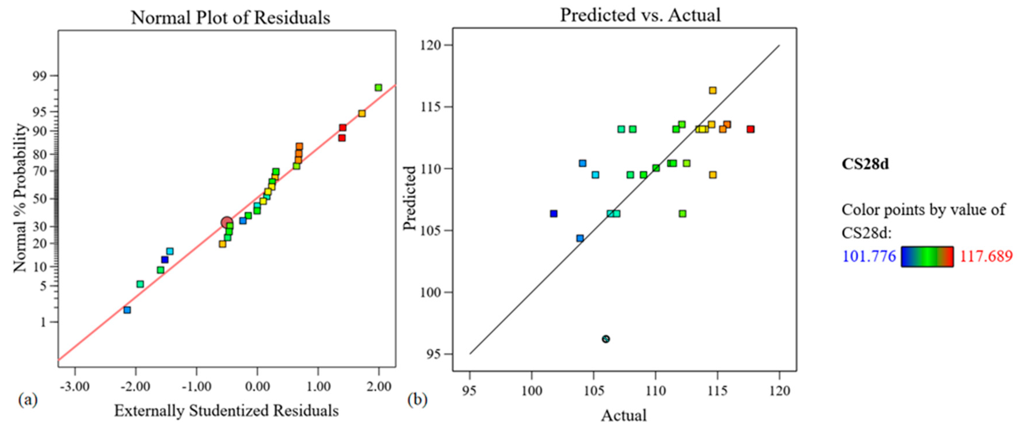
3.5. Regression Model for 28-Day Compressive Strength

The regression analysis seemed to suggest that quadratic models were the most promising candidates. However, upon ANOVA analysis, the quadratic model was found to be nonsignificant, as the p-value was 0.2889 and therefore under the recommended threshold of 0.05. Among the terms examined, only A² exhibited statistical significance, with a p-value of 0.0252, while all the other terms (A, B, C, D, AB, AD, BC, BD, CD, B², C², and D²) were found to be not significant. Moreover, the predicted R² was found to be −0.8825, with an adjusted R² of 0.1506. This substantial discrepancy suggests that the quadratic model’s efficacy was low. Graphic diagnosis was conducted and revealed a potential outlier at Std 18, Run 20, which was clearly shown by the distribution in the Predicted versus Actual plot, the Residual versus Predicted plot, the Residual versus Factor plot, and the Cook’s distance relationships (not show here for the sake clarity). This data point exceeded the DFFITS limit and was consequently excluded from subsequent analysis. Still, these results suggested that the quadratic model could be reduced (by removing some terms) to enhance its significance.

Table 10. Fitting results for compressive strength results after 28 days of curing.

Source	Sum of Squares	Mean Square	F-Value	p-Value
Model	239.43	79.81	6.99	<0.0015
A—w/c	72.33	72.33	6.33	<0.0189
D—s/m	59.12	59.12	5.18	0.0321
A²	161.61	161.61	14.15	0.0010
Residual	274.10	11.42
Lack of Fit	201.81	10.09	0.5584	0.8297
Pure Error	72.29	18.07
Cor Total	513.53	-

shows the fitting results for the regression model compressive strength after removing the terms B, C, AB, AC, AD, BC, BD, CD, B², C², and D².

The likelihood of such a high F-value occurring due to noise was only 0.15%. Therefore, the quadratic model was directionally reduced to address the presence of insignificant terms and to ensure statistical significance. The significant terms A, D, and A² were retained. The newly built model had a nonsignificant lack of fit, with an 82.97% probability that misfit could be attributable to noise. The predicted R² value of 30.89% exhibited reasonable agreement with the adjusted R² value of 39.95%, with a difference of less than 20%. Adequate precision was measured, with a value of 9.366, which indicates that the signal was sufficiently strong and the model was well-suited to describe the design space.

Table 11. Coefficients in terms of coded factors—compressive strength after 28 days of curing.

Factor	Intercept	A-w/c	D-s/m	A²
Coefficient Estimate	113.19	−2.04	−1.57	−3.22
Standard Error	0.8726	0.8097	0.6898	0.8573
95% CI Low	111.39	−3.71	−2.99	−4.99
95% CI High	114.99	−0.3665	−0.1457	−1.46
VIF	-	1.14	1.00	1.14

presents the estimated coefficients for compressive strength after 28 days of curing, which all lay within the 95% confidence interval. The variance inflation factor (VIF) for the factors A and A² was 1.14, thereby indicating multicollinearity, while the variable D had a VIF of 1.0, thereby demonstrating orthogonality.

Figure 7a shows the normal plot of the residuals for the compressive strength model after excluding the data point Std 18, Run 20. One can observe that the data points appear distributed across a line, but a fully linear distribution is not entirely perceived. Figure 7b shows the Predicted versus Actual relationship plot. The data point that was excluded is clearly noticeable in the lower quadrant of Figure 7b. In Figure 7b, one can also observe that the data points tended to distribute along a straight line; however, they exhibited some dispersion due to the moderate/low coefficient of determination (R²).

4. Discussion

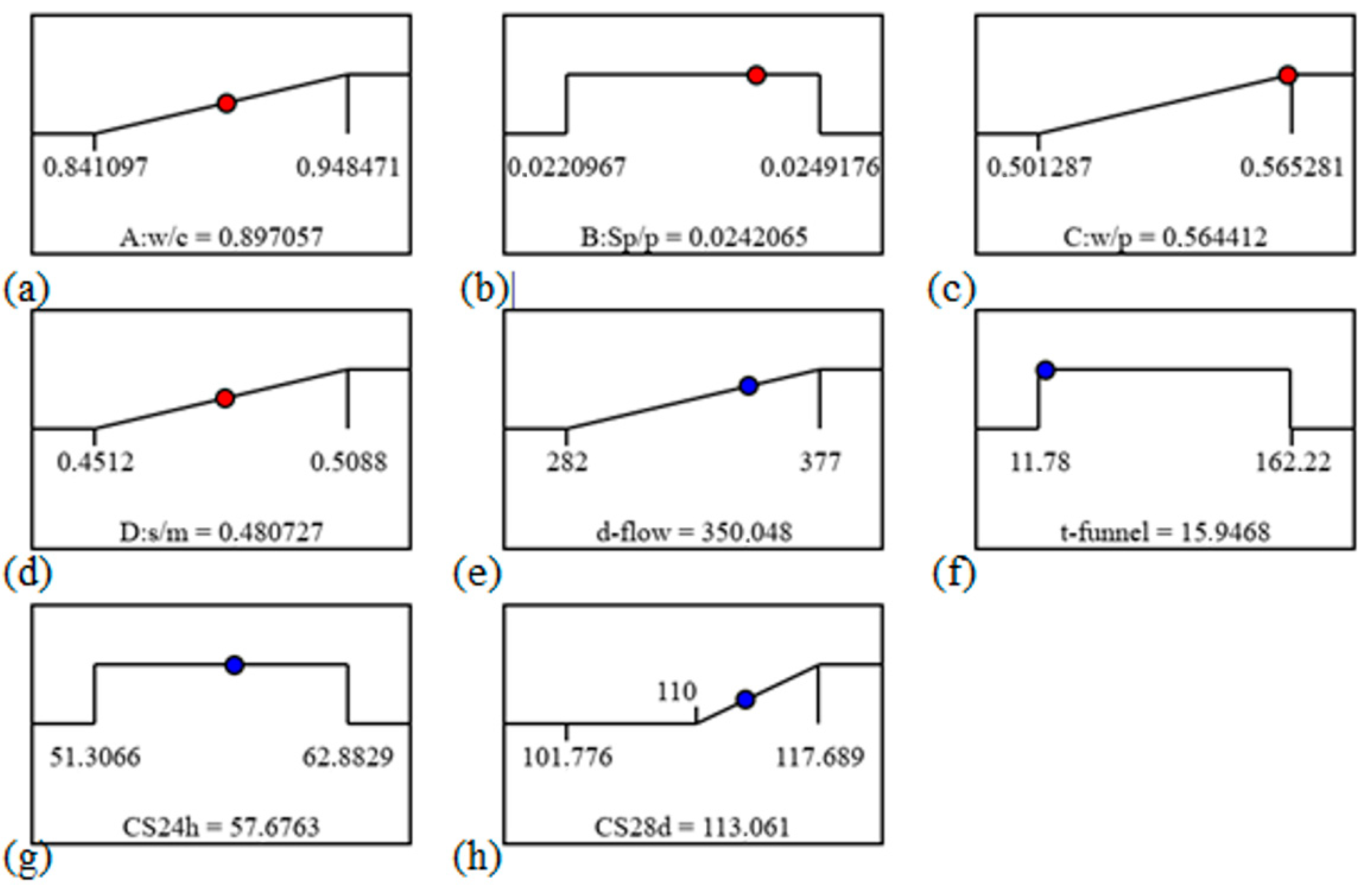
4.1. Model Optimization

After finding the ideal models for each of the self-compacting mortar variables, through a central composite design, the model was optimized in order to find the best solutions based on certain criteria. Targets were set for each input and output variable, thereby encompassing maximization, minimization, achieving specific values, or falling within delimited intervals. The established limits for each variable were based on the database comprising 30 mixtures. In addition, weights ranging from 0.1 to 10 were defined (with the default being 1), along with a degree of importance ranging from 1 plus (+) to 5 plus (+++++). This approach adheres to the methodology proposed by Myers, Montgomery, and Anderson-Cook [42], who aimed to maximize global desirability across a set of output variables.

This study sought to identify mortar compositions that met the following criteria: (i) developed a higher compressive strength at 28 days with the lowest possible cement content to reduce production costs and environmental impacts and (ii) featured a high workability in order to facilitate the flow and ease of consolidation of the mixtures in slender structures and/or in highly reinforced arrangements.

Table 12. Determined criteria to optimize the mix.

Factor	Goal	Lower Limit	Upper Limit	Weight	Importance
A: w/c	To be maximized	0.8411	0.9485	1	+++++
B: Sp/p	To be in range	0.0221	0.0249	1	+++
C: w/p	To be maximized	0.5013	0.5653	1	+++++
D: s/m	To be maximized	0.4512	0.5088	1	+++++
Y1: D-Flow (mm)	To be maximized	282	377	1	++++
Y2: T-Funnel (s)	To be in range	11.78	162.22	1	+++
Y3: CS24h (MPa)	To be in range	51.3066	62.88	1	+++
Y4: CS28d (MPa)	To be maximized	110.00	117.69	1	+++++

presents the criteria for optimizing high-strength self-compacting mortars. For the input variable A (w/c), the objective was to minimize cement consumption; hence, a maximization goal was defined, with a weight of one and a maximum importance (factor 5 = +++++). For the input variable C (w/p), the objective was to maximize the water content over the powder content, and it was also assigned the same importance as factor A but with a weight of one. As for the variable D (s/m), maximizing it allowed for reducing the consumption of mortar in relation to sand, thus further contributing to reducing costs and the environmental impacts.

To increase the flowability of the self-compacting mortars and to optimize their performance during the concreting of slender elements with high reinforcement rates, the response variable Y1 (D-Flow) needed to be maximized and was ascribed a degree of importance of four. However, the maximum degree of importance was attributed to variable Y4, thereby aiming to maximize the compressive strength after 28 days with a minimum acceptance criterion of 110 MPa. The establishment of a minimum compressive strength criterion was envisioned to attain values surpassing the sample’s average. Variables B (Sp/p), Y2 (T-Funnel), and Y3 (compressive strength after 24 h) were deemed to remain within acceptable value ranges, with a moderate degree of importance being attributed. After computing, a comprehensive set of 85 candidate solutions was found.

Table 13. The top five optimized mortar formulations according to global desirability scores.

Factor	1	2	3	4	5
A: w/c	0.897	0.904	0.889	0.889	0.878
B: Sp/p	0.024	0.023	0.024	0.024	0.023
C: w/p	0.564	0.563	0.561	0.555	0.564
D: s/m	0.481	0.4894	0.499	0.495	0.485
Y1: D-Flow (mm)	350.05	342.67	336.12	334.94	341.24
Y2: T-Funnel (s)	15.95	17.46	19.79	20.22	18.10
Y3: CS24h (MPa)	57.68	57.37	58.32	58.44	58.80
Y4: CS28d (MPa)	113.06	112.27	112.35	112.57	113.27
Desirability	0.591	0.586	0.570	0.555	0.549

summarizes the top five optimized mixtures ranked based on their global desirability scores.

Figure 8 shows the desirability ramps of the different factors and responses for the candidate solution 1. It is observed that the input factors A, C, and D can be maximized without compromising the main objective of increasing the output variable Y4 (CS28d). Variable Y1 (D-Flow) attained its highest value of 343.3 mm, yet it still remained within the specified range of 282 to 377 mm. Factor B and output variables Y2 and Y3 adhered to the designated intervals, thereby aligning with the predefined criteria.

4.2. Optimization of Self-Compacting Mortars Using Response Surface Methodology

Response surface methodology (RSM) is a valuable tool that enables the establishment of relationships between independent variables and corresponding responses, thereby facilitating the optimization of mixed designs to achieve envisioned target features. Through RSM, plots are generated to visually illustrate the influence of each variable, which are represented by slopes or curvatures. Figure 9 shows the relationship between each output response and two of its key governing input variables.

Figure 9a shows the influence of A (w/c) and B (Sp/p) on Y1 (D-Flow). It is clear that increasing the w/c and Sp/p led to higher fluidity. This can be attributed to the higher amount of water in the system and the lower cement content when variable A increased, in addition to the greater amount of superplasticizer used in relation to powder, thus contributing to greater fluidity. Figure 9b shows how variables A (w/c) and D (s/m) are related to the response variable Y2 (T-Funnel). The reduction of the w/c factor (A) increased the funnel time due to the decrease in the amount of water in relation to the cement. In addition, with the increase in the D factor (s/m), the amount of sand increased in relation to the mortar, thus increasing the T-Funnel.

Figure 9c shows Y3 as a function of A and D. A strong inverse relationship can be observed between variable A and response Y3, thereby demonstrating that decreasing the w/c enhanced the compressive strength at 24 h of curing. However, for variable D, there was a minor increase in the s/m factor when the response variable was increased. Nevertheless, only variables A and D were shown to be related; the other variables promoted the following influences: regardless of the variation in B (Sp/p), there were insignificant changes in the Y3 response (CS24h), while, as there was an increase in the variable C (s/m), the CS24h also increased.

The temporal evolution of the strength development as a function of A and D can be depicted by observing the difference between Figure 9c and Figure 9d. The previously straight surface became curved. The curvature occurred mainly in A, as decreasing the w/c resulted in an increased compressive strength at 28 days (Y4). However, the observed growth was not continuous, as the highest values of the CS28d were present in the third quadrant, which is shown in Figure 9 (between 0.86794 and 0.894784). In addition, an upward slope can be observed on the D axis, thereby indicating that decreasing the variable D resulted in a higher compressive strength at 28 days, especially at low w/c ratios.

These results suggest that, as curing time increases, the relationship between the two input variables A (w/c) and D (s/m) with the output Y4 (CS28d) also increases, most notably with variable D (s/m). Variables B (Sp/p) and C (w/p) were not tested here, since they did not show relevant interference for the response factor Y4 (CS28d).

5. Conclusions

The studies conducted in this work aimed to identify significant models that were capable of optimizing the performance of self-compacting mortars and to evaluate the influence of different model parameters on the prediction accuracy. Response surface methodology (RSM) and central composite design were employed as effective tools for modeling the fresh state properties and strength development, thereby resulting in the following conclusions:

Following refinements, the D-Flow linear model emerged as a commendably well-fitted model, which was characterized by an elevated adjusted determination coefficient of 87.4%. In addition, the residual normal and predicted versus actual plots revealed good correlations, thereby demonstrating the model’s statistical significance.

Of note, an inverse transform was applied to the T-Funnel model, which yielded an enhanced adjusted determination coefficient of 93.3%. The coherence between the predicted and empirical outcomes testifies to the model’s precision and validity.

The outlier exclusion yielded a well-fitted CS24h model with an adjusted R² of 79.1%, a low standard deviation, and good correction coefficients. The ideal model was found to be a linear reduction with the omission of variable B, which was dictated by its negligible significance. The CS28d model was found to be statistically significant despite a moderated adjusted R² of 39.9%, thus showcasing the potential actions for future improvements. The expeditions in model determination and material optimization have shown the pivotal roles of the variables A and C in shaping the D-Flow and T-Funnel responses, thus further demonstrating the relevance of the w/c ratio, which is an influencer that transcended the response categories.

This pioneering research advances the comprehension of the statistical methodologies within the scope of civil engineering and construction materials, and it is particularly relevant in the development of advanced self-compacting cement-based products. The successful exploration of the proposed models further elucidates a roadmap for forthcoming explorations, with the potential to reduce production costs, curtail environmental impacts, and increase the technical performance of advanced self-compacting mortars.

References

1. Ali, M.; Kumar, A.; Yvaz, A.; Salah, B. Central composite design application in the optimization of the effect of pumice stone on lightweight concrete properties using RSM. Case Stud. Constr. Mater. 2023, 18, e01958. [Google Scholar] [CrossRef]
2. Rashid, K.; Farooq, S.; Mahmood, A.; Iftikhar, S.; Ahmad, A. Moving towards resource conservation by automated prioritization of concrete mix design. Constr. Build. Mater. 2020, 236, 117586. [Google Scholar] [CrossRef]
3. Okamura, H.; Ouchi, M. Self-compacting high performance concrete. Prog. Struct. Eng. Mater. 1998, 1, 378–383. [Google Scholar] [CrossRef]
4. Shi, C.; Wu, Z.; Lv, K.; Wu, L. A review on mixture design methods for self-compacting concrete. Constr. Build. Mater. 2015, 84, 387–398. [Google Scholar] [CrossRef]
5. De Schutter, G.; Bartos, P.J.; Domone, P.; Gibbs, J. Self-Compacting Concrete (Vol. 288); Whittles Publishing: Caithness, The Netherlands, 2018; Available online: http://hdl.handle.net/1854/LU-689512 (accessed on 20 July 2023).
6. Okamura, H.; Ouchi, M. Self-Compacting Concrete. J. Adv. Concr. Technol. 2003, 1, 5–15. [Google Scholar] [CrossRef]
7. Aitcin, P.C. Concreto de Alto Desempenho, 1st ed.; Pini: São Paulo, Brazil, 2000. [Google Scholar]
8. Beersaerts, G.; Ascensão, G.; Pontikes, Y. Modifying the pore size distribution in Fe-rich inorganic polymer mortars: An effective shrinkage mitigation strategy. Cem. Concr. Res. 2021, 141, 106330. [Google Scholar] [CrossRef]
9. Petrou, A.K.M.F.; Ioannou, I. Durability performance of self-compacting concrete. Constr. Build. Mater. 2012, 37, 320–325. [Google Scholar]
10. Nuruzzaman; Ahmad, T.; Sarker, P.K.; Shaikh, F.U.A. Rheological behaviour, hydration, and microstructure of self-compacting concrete incorporating ground ferronickel slag as partial cement replacement. J. Build. Eng. 2023, 68, 106127. [Google Scholar] [CrossRef]
11. Zerbino, R.; Barragán, B.; Garcia, T.; Agulló, L.; Gettu, R. Workability tests and rheological parameters in self-compacting con-crete. Mater. Struct. Constr. 2009, 42, 947–960. [Google Scholar] [CrossRef]
12. Ascensão, G.; Marchi, M.; Segata, M.; Faleschini, F.; Pontikes, Y. Reaction kinetics and structural analysis of alkali activated Fe–Si–Ca rich materials. J. Clean. Prod. 2020, 246, 119065. [Google Scholar] [CrossRef]
13. Upasani, R.S.; Banga, A.K. Response Surface Methodology to Investigate the Iontophoretic Delivery of Tacrine Hydrochloride. Pharm. Res. 2004, 21, 2293–2299. [Google Scholar] [CrossRef] [PubMed]
14. Montgomery, D.C. Design and Analysis of Experiments; John Wiley: Hoboken, NJ, USA, 2017. [Google Scholar]
15. Box, K.B.; Wilson, G.E.P. On the experimental attainment of optimum conditions. J. R. Stat. Soc. 1951, 1–38. [Google Scholar] [CrossRef]
16. Box, J.S.; Hunter, G.E.P.; Hunter, W.G. Statistics for Experimenters: An Introduction to Design, Data Analysis and Model Building; Wiley: New York, NY, USA, 1978. [Google Scholar]
17. Awolusi, T.; Oke, O.; Akinkurolere, O.; Sojobi, A. Application of response surface methodology: Predicting and optimizing the properties of concrete containing steel fibre extracted from waste tires with limestone powder as filler. Case Stud. Constr. Mater. 2019, 10, e00212. [Google Scholar] [CrossRef]
18. Ali, M.; Khan, M.I.; Masood, F.; Alsulami, B.T.; Bouallegue, B.; Nawaz, R.; Fediuk, R. Central composite design application in the optimization of the effect of waste foundry sand on concrete properties using RSM. Structures 2022, 46, 1581–1594. [Google Scholar] [CrossRef]
19. Khan, M.I.; Sutanto, M.H.; Bin Napiah, M.; Khan, K.; Rafiq, W. Design optimization and statistical modeling of cementitious grout containing irradiated plastic waste and silica fume using response surface methodology. Constr. Build. Mater. 2021, 271, 121504. [Google Scholar] [CrossRef]
20. Ghafari, E.; Costa, H.; Júlio, E. RSM-based model to predict the performance of self-compacting UHPC reinforced with hybrid steel micro-fibers. Constr. Build. Mater. 2014, 66, 375–383. [Google Scholar] [CrossRef]
21. Dahish, H.A.; Almutairi, A.D. Effect of elevated temperatures on the compressive strength of nano-silica and nano-clay modified concretes using response surface methodology. Case Stud. Constr. Mater. 2023, 18, e02032. [Google Scholar] [CrossRef]
22. Mohammed, B.S.; Fang, O.C.; Hossain, K.M.A.; Lachemi, M. Mix proportioning of concrete containing paper mill residuals using response surface methodology. Constr. Build. Mater. 2012, 35, 63–68. [Google Scholar] [CrossRef]
23. Nunes, S.; Matos, A.M.; Duarte, T.; Figueiras, H.; Sousa-Coutinho, J. Mixture design of self-compacting glass mortar. Cem. Concr. Compos. 2013, 43, 1–11. [Google Scholar] [CrossRef]
24. Keleştemur, O.; Yildiz, S.; Gökçer, B.; Arici, E. Statistical analysis for freeze–thaw resistance of cement mortars containing marble dust and glass fiber. Mater. Des. 2014, 60, 548–555. [Google Scholar] [CrossRef]
25. Ferdosian, I.; Camões, A. Eco-efficient ultra-high performance concrete development by means of response surface methodology. Cem. Concr. Compos. 2017, 84, 146–156. [Google Scholar] [CrossRef]
26. Mermerdaş, K.; Algın, Z.; Oleiwi, S.M.; Nassani, D.E. Optimization of lightweight GGBFS and FA geopolymer mortars by response surface method. Constr. Build. Mater. 2017, 139, 159–171. [Google Scholar] [CrossRef]
27. Zahid, M.; Shafiq, N.; Isa, M.H.; Gil, L. Statistical modeling and mix design optimization of fly ash based engineered geopolymer composite using response surface methodology. J. Clean. Prod. 2018, 194, 483–498. [Google Scholar] [CrossRef]
28. Matos, A.M.; Maia, L.; Nunes, S.; Milheiro-Oliveira, P. Design of self-compacting high-performance concrete: Study of mortar phase. Constr. Build. Mater. 2018, 167, 617–630. [Google Scholar] [CrossRef]
29. Khan, M.I.; Sutanto, M.H.; Napiah, M.B.; Zahid, M.; Usman, A. Optimization of Cementitious Grouts for Semi-Flexible Pavement Surfaces Using Response Surface Methodology. IOP Conf. Ser. Earth Environ. Sci. 2020, 498, 012004. [Google Scholar] [CrossRef]
30. Al Salaheen, M.; Alaloul, W.S.; Malkawi, A.B.; de Brito, J.; Alzubi, K.M.; Al-Sabaeei, A.M.; Alnarabiji, M.S. Modelling and Optimization for Mortar Compressive Strength Incorporating Heat-Treated Fly Oil Shale Ash as an Effective Supplementary Cementitious Material Using Response Surface Methodology. Materials 2022, 15, 6538. [Google Scholar] [CrossRef]
31. Shi, X.; Zhang, C.; Wang, X.; Zhang, T.; Wang, Q. Response surface methodology for multi-objective optimization of fly ash-GGBS based geopolymer mortar. Constr. Build. Mater. 2022, 315, 125644. [Google Scholar] [CrossRef]
32. Anurag; Singh, S. Estimation of the impacts of adding recycled demolition waste and steel fibers on different mechanical properties of self-compacting concrete. Mater. Today Proc. 2022, 48, 1723–1730. [Google Scholar] [CrossRef]
33. Waqar, A.; Bheel, N.; Almujibah, H.R.; Benjeddou, O.; Alwetaishi, M.; Ahmad, M.; Sabri, M.M.S. Effect of Coir Fibre Ash (CFA) on the strengths, modulus of elasticity and embodied carbon of concrete using response surface methodology (RSM) and optimization. Results Eng. 2023, 17, 100883. [Google Scholar] [CrossRef]
34. Khavari, B.C.; Shekarriz, M.; Aminnejad, B.; Lork, A.; Vahdani, S. Laboratory evaluation and optimization of mechanical properties of sulfur concrete reinforced with micro and macro steel fibers via response surface methodology. Constr. Build. Mater. 2023, 384, 131434. [Google Scholar] [CrossRef]
35. Hamada, H.M.; Al-Attar, A.A.; Tayeh, B.; Yahaya, F.B.M.; Abu Aisheh, Y.I. Optimising concrete containing palm oil clinker and palm oil fuel ash using response surface method. Ain Shams Eng. J. 2023, 14, 102150. [Google Scholar] [CrossRef]
36. Mita, A.F.; Ray, S.; Haque, M.; Saikat, H. Prediction and optimization of properties of concrete containing crushed stone dust and nylon fiber using response surface methodology. Heliyon 2023, 9, e14436. [Google Scholar] [CrossRef]
37. Sinkhonde, D. Generating response surface models for optimisation of CO2 emission and properties of concrete modified with waste materials. Clean. Mater. 2022, 6, 100146. [Google Scholar] [CrossRef]
38. Adamu, M.; Trabanpruek, P.; Jongvivatsakul, P.; Likitlersuang, S.; Iwanami, M. Mechanical performance and optimization of high-volume fly ash concrete containing plastic wastes and graphene nanoplatelets using response surface methodology. Constr. Build. Mater. 2021, 308, 125085. [Google Scholar] [CrossRef]
39. Li, L.; Wan, Y.; Chen, S.; Tian, W.; Long, W.; Song, J. Prediction of optimal ranges of mix ratio of self-compacting mortars (SCMs) based on response surface method (RSM). Constr. Build. Mater. 2022, 319, 126043. [Google Scholar] [CrossRef]
40. Safhi, A.e.M.; Benzerzour, M.; Rivard, P.; Abriak, N.-E.; Ennahal, I. Development of self-compacting mortars based on treated marine sediments. J. Build. Eng. 2019, 22, 252–261. [Google Scholar] [CrossRef]
41. Maia, L. Experimental dataset from a central composite design with two qualitative independent variables to develop high strength mortars with self-compacting properties. Data Brief 2021, 40, 107738. [Google Scholar] [CrossRef] [PubMed]
42. Myers, R.H.; Montgomery, D.C.; Anderson-Cook, C.M. Response Surface Methodology, 3rd ed.; Wiley: New York, NY, USA, 2009. [Google Scholar]
Figure 1. Heatmap of correlations between input and output variables. Darker colors indicate stronger correlations, with red and blue differentiating positive and negative relationships, respectively.
Applsci 13 10428 g001
Figure 2. Normal probability of residuals (a) and Residuals versus Run plot (b) for D-Flow model. Arrows included to highlight outlier data point.
Applsci 13 10428 g002
Figure 3. Plot of the normal probability of residuals for the D-Flow model (a) and Residuals versus Predicted plot for the D-Flow model (b); both plotted after the initial fitting.
Applsci 13 10428 g003
Figure 4. Graphs for D-Flow model: (a) Normal Plot of Residuals; (b) Residuals versus Run; and (c) Predicted versus Actual.
Applsci 13 10428 g004
Figure 5. T-Funnel linear model: (a) Normal Plot of Residuals; (b) Residuals versus Run; (c) Box–Cox for Power Transforms; and (d) Predicted versus Actual.
Applsci 13 10428 g005
Figure 6. Regression model for compressive strength after 24 h of curing: (a) Normal Plot of Residuals and (b) Predicted versus Actual.
Applsci 13 10428 g006
Figure 7. Graphs for CS28d model: (a) Normal Plot of Residuals and (b) Predicted versus Actual.
Applsci 13 10428 g007
Figure 8. Desirability ramps for numerical optimization of different input and output variables of the best candidate solution found: (a) A: w/c; (b) B: Sp/p; (c) C: w/p; (d) D: s/m; (e) Y1: D-Flow; (f) Y2: T-Funnel; (g) Y3: CS24h; and (h) Y4: CS28d.
Applsci 13 10428 g008
Figure 9. Rheological properties and strength development as a function of different variables: (a) D-Flow; (b) T-Funnel; compressive strength at 24 h (c); compressive strength after 28 days of curing (d).
Applsci 13 10428 g009