Spectroscopy Imaging Techniques as In Vivo Analytical Tools to Detect Plant Traits

Abstract

The efficiency of hyper- and multispectral imaging (HSI and MSI) has gained considerable attention in research on plant phenotyping. This is due to their ease of use while being considered a nondestructive technology. Unlike current point-scanned spectroscopy, both HSI and MSI extract spatial and spectral information while covering a wide range of a plant body. Moreover, it is necessary to equip the extracted information with multivariate calibration techniques, followed by model evaluation. To date, the application of HSI and MSI for monitoring plant growth under a controlled environment is emerging and showing a good trend. Our systematic literature review discusses spectroscopy imaging techniques and their chemometric approaches as a sustainable sensor technology to detect plant traits. In conclusion, we also explore the possibility of carrying out HSI and MSI during plant trait analysis.

1. Introduction

To date, the campaign to end hunger has received great attention from nations. With the growth in human population and the ongoing rise in food demand, hunger is a pertinent subject that warrants concern. Furthermore, the global population is expected to continue rising and eventually reach nine billion people [1]. Moreover, a meta-analysis investigated by Dijk et al. [2] demonstrated that there will be a rise in food consumption through 2050.

Although crop yields are projected to rise, concerns regarding food security and food safety have been spreading around the globe [3]. Coronavirus disease (COVID-19) and the war in Ukraine were the pressing problems in 2020–2022, leading to a loss of food security [4]. The challenge of food security appeared when people tried to deal with social distancing, which forced citizens to stay at home. In this case, people tended to store up their food shelves in huge amounts. Additionally, the fear of viral infection could heighten the concern about food unavailability [5] caused by inadequate access to agricultural activities. Similarly, the war between Russia and Ukraine significantly affects agricultural processes, from plant growth to food markets [6]. Further, food safety deals with the safety of the food production line, ranging from on-farm to off-farm practices [7,8]. Hazards commonly occur due to chemical contamination [9], physical contamination [10,11], food adulteration [12,13], genetic modification [14], and other processes. Chemical contamination and food adulteration in agricultural products are present as the side effects of food unavailability. Hence, an analytical method, such as spectroscopy, can be used. Spectroscopy imaging techniques are emerging as a powerful tool to directly and rapidly assess food quality [15], although a model needs to be built using machine learning algorithms before an assessment is conducted. We suggest the reviews by Gowen et al. [16] and Qin et al. [15] for detailed applications of spectroscopy imaging techniques in food safety control assessment. A description of current spectroscopy imaging techniques is available in Section 3.

Plants are considered one of the important food resources for humans and stocks. The consumption of plants can offer various advantages for the human body. This is due to the presence of natural materials in plants, such as vitamins, minerals, and other micro- and macronutrients. However, the quality of food products derived from plants depends on the unique traits during their growth period. Abiotic stresses, such as high salinity [17,18], extreme temperature [19,20], and drought [21,22], play a role in causing yield loss [23,24]. Nevertheless, these factors are present naturally during crop growth. Subsequently, numerous symptoms and alterations may occur throughout the growth time and, hence, plant growth can be disturbed. Plant biotechnology has been widely developed by researchers to strengthen various crops’ resistance to stresses, such as Chinese cabbage [25] and potato [26]. The term hybridization refers to combining high-resistance and high-yield genes with a target gene [27,28]. In this process, a technician is needed to isolate the desired gene and subsequently clone it to the target plant. Nevertheless, some Asian countries still face difficulties when confronting abiotic stresses that threaten crops, for example, heat stress during summer in countries such as Indonesia. In this case, due to the consequences of heat stress, plants are likely to show different responses (in physiological and biochemical aspects), as previously summarized by Hasanuzzaman et al. [29]. Under an elevating ambient temperature, the stomata tend to close and produce a lot of carbon dioxide, and the photosynthetic rate will fall gradually [30,31]. For an in-depth understanding, readers may refer to [29,30]. Therefore, a preventive step—crop growth monitoring—should be conducted [32].

At present, the use of spectroscopy imaging technologies, hyper- and multispectral imaging (HSI and MSI), is more favored than the manual technique. The reason is due to their ease of use while being rapid and nondestructive. Nondestructive refers to the ability to reuse samples without damaging them during analysis. In contrast, chromatography tools, namely gas chromatography [33] and liquid chromatography [33,34], require a lot of sample preparation and are time-consuming [35]. In such a way, destructive steps need to be performed, including drying, grinding, and extracting before injecting into the instrument [36]. In agriculture, research on HSI and MSI has been extensively conducted. Some of the publications related to the application of HSI and MSI are listed in

Table 1. Application of HSI and MSI in agriculture.

Research Emphasis	Refs.
Seed viability	[37,38]
Chemical compounds	[39,40,41]
Food adulteration	[10,42]
Food classification	[43,44,45,46,47,48]

.

Besides the above cited publications, HSI and MSI are also applicative for monitoring plant growth status. Plant phenotyping is still believed to be time-consuming and labor-intensive work [49]. The use of HSI and MSI can provide the physical and chemical features of plants [50] based on their reflectance/absorbance profiles. In this study, we present a systematic literature review of the application of HSI and MSI to monitor plant growth status according to the natural problems encountered by plants. We also provide (i) general information on plant traits; (ii) the interaction of light and plants; (iii) data analyses; and (iv) recent trends of HSI and MSI for monitoring plant growth status. For the review, we collected published papers from Google Scholar with the keywords, “plant abiotic/biotic stress detection using hyperspectral and multispectral imaging”, in 2010–2023.

2. Plant–Light Interaction

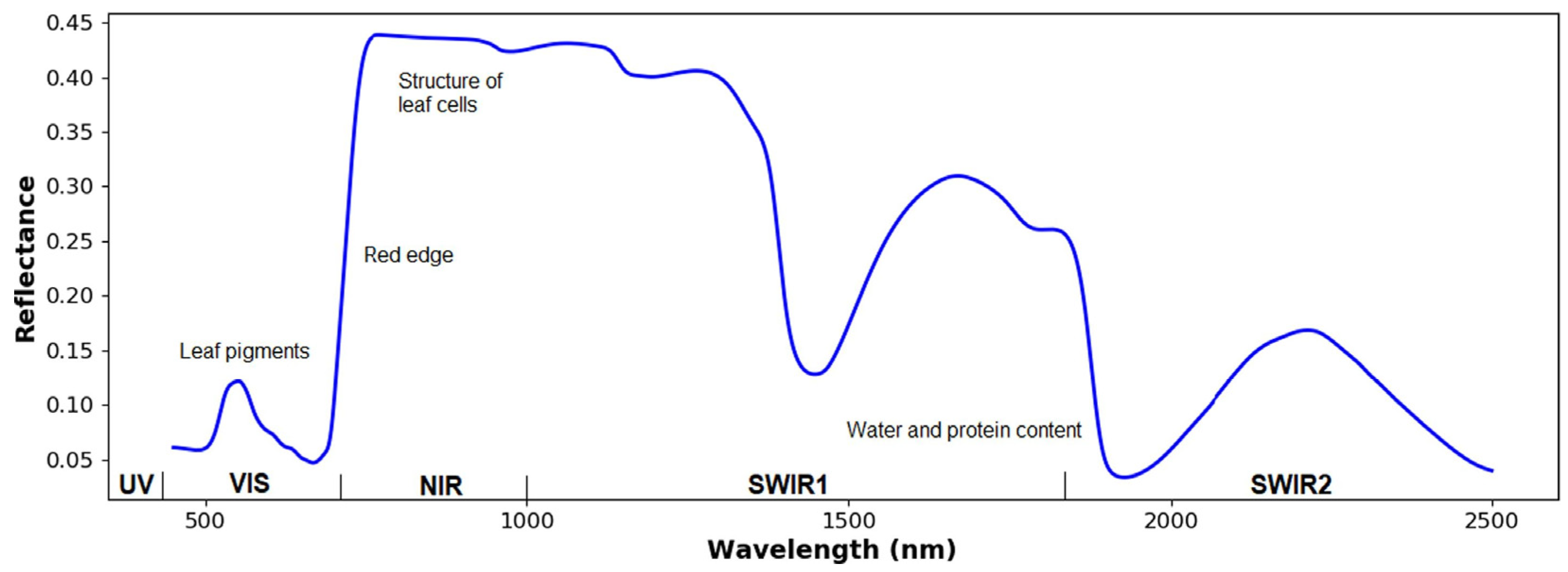
To begin, an HSI and MSI system involves analyzing light–plant interaction. Understanding this interaction can help choose the proper sensor [51]. Light (electromagnetic radiation, EMR) and plant interaction depends on light frequencies [50]. For healthy leaves, photosynthetic pigments, e.g., chlorophyll, carotenoids, anthocyanin, and xanthophyll, can be observed in the VIS region (400–700 nm), while the NIR region (700–1100 nm) predominantly corresponds to dry matter, and the SWIR region, within 1100–2500 nm, is mainly attributed to water [50]. Sarić et al. [52] stated that nitrogen and water can also be observed in the NIR and SWIR regions, respectively. As shown in Figure 1, the visible region has a lower reflection value. This is caused by the highest absorption at approximately 490 and 690 nm by chlorophyll [53]. A small peak reflection is also observed in the visible range (~550 nm), which contributes to the green color [54]. In the NIR bands, a high–sharp reflectance trend occurs, indicating a red edge, in which light absorption by leaf pigments no longer exists [54,55]. In vegetables, the response of O–H bands is found at 1190, 1450, and 1940 nm [10]. The absorption of the first overtone of carbon–hydrogen bond could be detected between 1700 and 1800 nm [56,57]. According to Tunny et al. [10], the response of C–H might be due to the presence of cellulose.

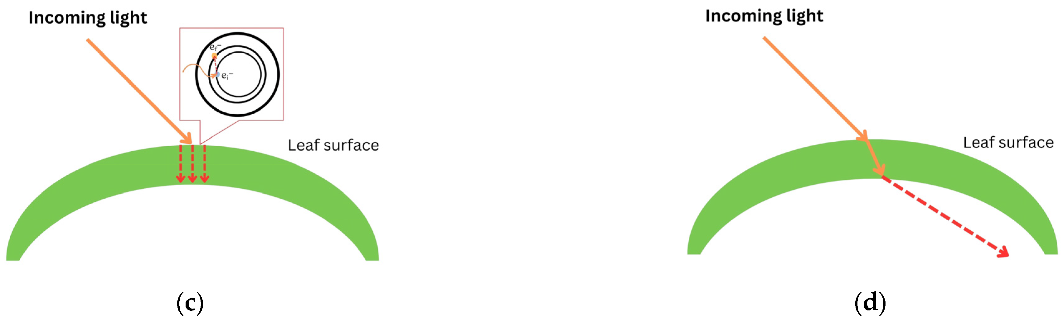
When light passes through a leaf, there will be some interactions between the plant and light. The interactions include (i) reflection, (ii) scattering, (iii) absorption, and (iv) transmission [50,52]. Reflection occurs when light is bounced back after entering the leaf’s surface. When light is reflected by a different angle caused by a different shape of the leaf structure, it is called scattering. In terms of absorption (mathematically described as $\mathrm{Log}1/\mathrm{R}$), electrons accept photons’ whole energy and are displaced to a higher configuration in the form of thermal energy. Otherwise, transmission occurs when atoms pick up the wave, vibrate briefly, transmit the vibration through the body of the leaf, and emit the wave as light at the other end. Figure 2 illustrates how light interacts with a leaf surface.

3. Hyper- and Multispectral Imaging

It is nearly impossible to monitor a crop’s status through the naked eye. The human eye is limited in its ability to measure or quantify due to fatigue. Consequently, bias results may occur. Moreover, manual laboratory analyses require highly skilled technicians and are time-consuming. Thus, the utilization of nondestructive technologies, such as HSI and MSI, is a promising tool. It offers numerous beneficial aspects, such as being nondestructive and noninvasive with rapid inspection [15]. Due to its advantages, the use of HSI and MSI has become a necessity. HSI and MSI offer both spatial and spectral information [40,52,58,59,60]. For a review of the variability in illumination and camera type, readers can refer to [49]. To ease readers into the topic, we provide an illustration of HSI/MSI during data collection in Figure 3.

In terms of application, HSI is used for fundamental research and MSI is more applicable in field works [15]. In addition, HSI provides high resolution but is time-consuming compared to MSI. To apply MSI, HSI should be performed first to obtain the optimum wavebands [15]. According to Qin et al. [15], there are three scanning methods to acquire 3D hyperspectral cubes, namely (i) point scan, (ii) line scan, and (iii) area scan, as presented in Figure 4. Point scan obtains single-point spatial information by collecting each pixel. This method is time-consuming since it captures two spatial dimensions (x, y). Furthermore, point scan does not cover a wide area. Secondly, line scan is an extension of the former scanning method and captures slit spatial information. This method is suitable for moving samples, i.e., sortation. Additionally, the area scan method instantly captures 2D single-band grayscale images with full spatial information. Moreover, if the target object has undesirable movement, the HSI method is acceptable. In contrast, line and area scans are more suitable for MSI than point scan [15]. Line scan only works for the selected tracks during scanning time. Finally, area scan is fast and collects images at various wavelengths at once.

3.1. Spectral Correction

During data acquisition, some external disturbances, such as dark noises, unwanted light intensity, and environmental factors, might occur [32,40,42,61,62]. Commonly, before performing the measurement, the white and black reference data should be measured [43]. The white reference is obtained using a white Teflon with ±99% reflectance, and the dark reference (±0% reflectance) can be obtained by covering the lens. Finally, the corrected image’s spectral feature is mathematically quantified using Equation (1):

$${\mathrm{I}}_{\mathrm{R}}=\frac{{\mathrm{I}}_{\mathrm{raw}}-{\mathrm{I}}_{\mathrm{black}}}{{\mathrm{I}}_{\mathrm{white}}-{\mathrm{I}}_{\mathrm{black}}}$$

(1)

where ${\mathrm{I}}_{\mathrm{raw}},{\mathrm{I}}_{\mathrm{white}}$, and ${\mathrm{I}}_{\mathrm{black}}$ refer to the raw scanned object, the white reference, and the dark reference reflectance, respectively.

The next step after spectral calibration is the selection of regions of interest (ROIs). During data acquisition, the captured images not only show the target plant as a research object but also the background. Therefore, it is necessary to eliminate the background pixels from the calibrated images [32].

3.2. Preprocessing

Due to the advantages of HSI and MSI, which have been mentioned above, the performance of both instruments is primarily affected by their sensitivity, calibration, physical mechanism, and the surroundings [63]. Spike is a common phenomenon that can be found within the spectrum body. It presents as extreme rise and fall waves. The complexity of plant geometrics, i.e., spherical, elliptic, wavy, or irregular shape, has made it necessary to correct images with preprocessing, which is inspired by chemometrics [50]. Firstly, the average of spectral data can be employed since averaging can reduce noises and correct the illumination effect [49]. In addition, spectral averaging is the simplest preprocessing method. This method has been successfully applied to predict the plant physiology and leaf water content of maize [64]; the water content, micro-, and macronutrients in maize and soybean [65]; and the water and nitrogen contents in wheat [66]. Secondly, other preprocessing techniques, namely multiplicative scatter correction (MSC) and standard normal variate (SNV), can be established to reduce variability due to scattering or baseline shift. Thirdly, smoothing by applying a Savitzky–Golay filter can also be established.

3.3. Chemometric Models

Hyper- and multispectral imaging generates reflectance values from each waveband. Nevertheless, it is indirectly applicable. Chemometrics is an analytical approach originally derived from statistical and mathematical concepts [67]. This analytical step is favorably employed by researchers to develop prediction models based on reflectance values. Chemometric techniques have been intensively carried out to predict the desired objectives within agri-food production lines, e.g., chemical content, food sensory, and plant monitoring status. Moreover, chemometrics also promotes simple presentation by reducing the dimension and complexity of large datasets, classifies samples, and enables data modeling, with robust accuracy [68].

Principal component analysis (PCA) has been successfully applied by many researchers as a tool to analyze spectral data. Since spectral data consist of numerical reflectance values for each waveband, dimensional reduction can be performed to display the information clearly in a two- or three-dimensional plot (called PCs). Although PCA simply presents variances in a scatter plot, it does not lose the information. PCA is also an acceptable method for observing outliers and constructing models. For instance, PCA clearly showed that adulterant materials had different reflectance values compared to fresh-cut vegetables [10]. Fresh-cut vegetables had a similar reflectance value, clustered together as a group, and were separated from adulterant materials. In another study, PCA was used to illustrate the contrast maps of chemical contents in different treated plants. In contrast, Lee et al. [69] reported that PCA had a lower coefficient of determination (R² = 0.69) in predicting total volatile basic nitrogen in pork. This was caused by the fact that PCA only obtained a single waveband (460 nm) to build the TVB-N prediction model.

At present, due to the high dimensionality of spectral data acquired using HSI/MSI, many researchers apply wavelength selection before performing chemometric analysis. The high dimensionality of HSI/MSI spectral data can be further reduced to a low dimension through feature extraction and feature selection. Feature extraction utilizes the original data, while feature selection requires class marking to choose the representative wavelength. However, wavelength extraction can remove intrinsic features [70].

In optical spectroscopy, outliers may occur during the data acquisition process. This phenomenon may be present due to the environment and operator errors [71,72]. Negatively, outlier samples can decrease the accuracy of the built predictive model. Therefore, outliers should be deselected before employing chemometrics. Principal component analysis (PCA) can detect such outliers. In a study by Pandey et al. [65], two-dimensional PC plots were used to figure out outliers. Since PCA can simply display clusters based on their similarity, sample outliers can easily be detected. Similarly, the effectiveness of PCA in tracing outliers had been proven previously [73].

To date, PLS-R has been intensively developed to establish predictive models of targeted components based on spectral features [74]. A latent variable—typically abbreviated as LV—is considered an important parameter to investigate the linear relatedness of both spectrum matrices and reference values. High accuracy of PLS-R depends on the number of chosen LV values, which is determined based on the lowest point of cross-validation root mean squared error [75]. Nevertheless, the accuracy of PLS-R relates to the validity of the reference matrices obtained using destructive methods. Generally, PLS-R itself is considered to be a linear regression and is mathematically described as shown below (Equation (3)). In Equation (2), $\mathrm{Y}$ is the reference value, $\mathrm{X}$ is the spectrum matrices ($\mathrm{m}\times \mathrm{n}$), $\mathrm{B}$ is the PLS-R coefficient, and $\mathrm{E}$ represents the error:

$$\mathrm{Y}=\mathrm{XB}+\mathrm{E}$$

(2)

Similar to PCA, PLS-R has the ability to reduce the high dimensionality of data matrices [67]. Practically, PLS-R has the ability to predict plant traits [76,77], food chemical contents [78], and other characteristics. In addition, various chemometric techniques, such as partial least squared discriminant analysis (PLS-DA), support vector machine regression (SVM-R), and least squared support vector machine (LS-SVM), can be applied.

Despite the development of the aforementioned chemometric techniques, at present, deep learning (DL) has been favorably developed and used for HSI/MSI data analysis. The concept of DL architecture imitates the principle of the human brain’s visual cortex. DL offers some advantages: (a) it discovers properties on its own; (b) it saves the process by reducing the need for computation; (c) it creates features manually; and (d) it uses large, annotated images that researchers already have access to [79]. However, supervised DL needs a large-scale dataset. In addition, DL-based spectroscopy is rarely used to quantify plant phenotypic features. Nevertheless, this method can automatically extract raw spectra and improve the performance of prediction models [80]. Hence, it is still possible to combine DL with spectroscopy during plant phenotyping. In

Table 2. Application of deep learning related to HSI/MSI for monitoring plant growth status.

Crop	Research Emphasis	Wavelength Range (nm)	Measurement Technique	DL Models **	Ref.
Cucumber	Leaf nitrogen prediction	400–1000	Hyperspectral imaging	ANN-PSO, PLSR, and CNN	[82]
Potato	Potato multi-defect detection	676–952	Multispectral imaging	YOLO-v5x, YOLOv3-tiny, DY2TNet, and MDDNet	[83]
Wheat	Fusarium head blight inspection	400–750	Hyperspectral imaging	DarkNet 19, EfficientNet B0 GoogLeNet MobileNet V2, ResNet 18 ResNet 50, ShuffleNet, and SqueezeNet	[84]
Lettuce	Plant biochemical features	400–1000	Hyperspectral imaging	2DCNN and FCNN	[80]
	Lead (Pb) detection within lettuce leaf	480.46–1001.61	Hyperspectral fluorescence imaging	WT-SAE and WT-MC-SAE	[85]
Citrus	Healthy and unhealthy leaf inspection	460, 520, 680, 740, 840, and 940	Multispectral reflectance imaging	Lightweight CNN (MobileNetV3) and transfer learning	[86]

** ANN-PSO = artificial neural network–particle swarm optimization; CNN = convolutional neural network; 2DCNN = two-dimensional convolutional neural network; FCNN = fully convolutional neural network; WT-SAE = wavelet transform coupled to stacked auto-encodes; WT-MC-SAE = Monte Carlo wavelet transform coupled to stacked auto-encodes.

, we summarize recent applications of DL for monitoring plant growth status. The detailed information of the use of deep learning in combination with spectroscopy can be found in Wang et al. [81]. Wang et al. [81] provides details of major types of DL (convolutional neural network/CNN, fully convolutional network/FCN, tensor learning model/TL, deep belief network/DBN, stacked auto-encoder/SAE, recurrent neural network/RNN, semi-supervised learning, generative adversarial network/GAN, and active learning model/AL) and challenges in the agricultural field.

3.4. Model Validation

Most researchers have commonly used a few mathematical formulas to evaluate the performance of their employed models. The importance is to establish that the proposed models show good satisfaction, as indicated by errors and/or linearity relationship. Based on our review, researchers have often conducted various chemometric methods in comparative study. For instance, different mask segmentations were performed to estimate chlorophyll contents in wheat using MSI combined with PLSR [87]; various models were applied to predict alfalfa yield using MSI [88]; and VI models were established to assess nitrogen status in winter oilseed rape using MSI [89]. The equations that are most commonly used are R-squared (${\mathrm{R}}^2$) and root mean squared error ($\mathrm{RMSE}$), which are expressed in Equations (3) and (4), respectively:

$${\mathrm{R}}^2=1-\frac{\sum _{\mathrm{i}=1}^{\mathrm{n}}{\left({\mathrm{y}}_{\mathrm{I},\mathrm{es}}-{\mathrm{y}}_{\mathrm{I},\mathrm{ref}}\right)}^2}{\sum _{\mathrm{i}=1}^{\mathrm{n}}{\left(\stackrel{\mathrm{-}}{\mathrm{y}}\text{–}{\mathrm{y}}_{\mathrm{I},\mathrm{es}}\right)}^2}$$

(3)

where $\mathrm{n}$ corresponds to the total dataset; ${\mathrm{y}}_{\mathrm{i},\mathrm{es}}$ and ${\mathrm{y}}_{\mathrm{i},\mathrm{ref}}$ refer to the estimated and referenced values at the $i$th element, respectively; and $\overline{y}$ is the average value of the reference data (destructive value). The value of ${\mathrm{R}}^2$ ranges between $-\text{∞}$ and 1 [90]. A model with the closest value to 1 has excellent goodness-of-fit performance. However, we do not recommend evaluating models based on ${\mathrm{R}}^2$ itself. This is due to the fact that ${\mathrm{R}}^2$ represents the connection between the $\mathrm{x}$-axis (reference) and $\mathrm{y}$-axis (predicted). Additionally, $\mathrm{RMSE}$ can be calculated to make the decision:

$$\mathrm{RMSE}=\sqrt{\frac{1}{\mathrm{n}}\sum _{\mathrm{i}=1}^{\mathrm{n}}{\left({\mathrm{y}}_{\mathrm{i},\mathrm{es}}-{\mathrm{y}}_{\mathrm{i},\mathrm{ref}}\right)}^2}$$

(4)

In contrast, the decision based on $\mathrm{RMSE}$ is in selecting a smaller value. Based on our literature review, a higher $\mathrm{RMSE}$ value is caused by a larger gap between the predicted and observed data. Thus, a higher $\mathrm{RMSE}$ indicates a poorly built model and, thus, it should not be chosen.

4. Trends of HSI/MSI in Monitoring Plant Growth Status

4.1. Drought/Water Stress

Water holds an essential role for any living organism. In addition, the presence of water during crop production can affect the productivity of crops. As reported by Ihuoma and Madramootoo [91], water stress triggers some metabolic processes, such as falling transpiration rate [92], decreasing evaporative cooling, and rising leaf temperature [93]. This phenomenon is primarily caused by stomatal closure. Moreover, the availability of water is strongly correlated with climate change [94].

According to Abid et al. [94], drought stress triggers several physiological and biochemical changes in wheat (Triticum aesticum L.). During the water stress treatments, it was discovered that the net photosynthesis rate (P_n) and stomatal conductance (g_s) fell moderately after the 5th and 10th day of stress. The declined net photosynthesis rate was primarily attributed to the lower stomatal conductance. Furthermore, CO₂ content also decreased along with the reduction in stomatal conductance. Similarly, the leaf pigment, carotenoid, also decreased. In contrast, water limitation led to a higher value for some chemical compounds in wheat leaf, such as proline content, amino acids, total soluble sugar, and fructose.

Table 3. Recent publications related to drought detection using HSI/MSI.

Plants	Instrument	Interest	Wavebands (nm)	Model	R2	RMSE	Accuracy (%)	Ref.
Apple (Malus domestica var. Buckeye Gala)	HSI (ImSpector V10E, Spectral Imaging, Oulu, Finland)	Water stress detection	385–1000	Vegetation indices (VIs)	N/A **	N/A	N/A	[95]
Barley (Hordeum vulfare L.)	HSI (SOC-700, Surface Optics Corps., San Diego, CA, USA)	Functional and structural leaf and canopy parameters	400–900	Simplex volume maximization (SiVM)	N/A	N/A	N/A	[96]
Soybean (cultivars William 82 and Houjaku Kuwazu)	HFSI * (VNIR Concentric Imaging Spectrograph, Headwall Photonics, Fitchburg, Massachusetts, MA, USA)	Drought stress	421–780	Partial least squared regression (PLS-R)	0.64–0.99	0.00–0.32	N/A	[97]
Soybean (Glycine max, Thorne variety)	HSI (Headwall Photonics, Fitchburg, Massachusetts, MA, USA)	Leaf chemical properties	550–1700	Partial least squared regression (PLS-R)	0.18–0.93	0.00–16.20	N/A	[65]
Maize (Zea mays)	HSI (AISA Eagle, Spectral Imaging, Oulu, Finland)	Relative water content, quantum yield of PSII †, differences between leaf and air temperatures, and leaf area index	400–992	Vegetation indices (VIs)	0.34–0.82	N/A	N/A	[98]
	HSI (Headwall Photonics, Fitchburg, Massachusetts, MA, USA)	Leaf water content	900–1700	Partial least squared regression (PLS-R)	0.81–0.92	2.3–3.7	N/A	[64]
	HSI (Headwall Photonics, Fitchburg, Massachusetts, MA, USA)	Leaf chemical properties	550–1700	Partial least squared regression (PLS-R)	0.18–0.93	0.00–16.20	N/A	[65]
Maize (Zea mays)	MSI (RedEdge multispectral camera, MicaSense Inc., Kansas, KS, USA)	Crop water stress index	475, 560, 668, 717, and 840	Vegetation indices (VIs)	0.27–0.81	0.037–0.066	N/A	[99]
	HSI (ImSpector V10E, Spectral Imaging, Oulu, Finland)	Water potential, effective quantum yield of PSII, stomatal conductance to H2O, and transpiration rate	500–850	Partial least squared regression (PLS-R)	0.76–0.91	0.071–0.12	N/A	[100]
				Kernel ridge regression (KRR)	0.82–0.92	0.065–0.11	N/A
				Gaussian process regression (GPR)	0.83–0.92	0.079–0.11	N/A
				Kernel ridge regression (KRR)	0.82–0.92	0.065–0.11	N/A
Vineyard	MSI (SEQUOIA multispectral sensors, Parrot Co., Ltd., Paris, France)	Water status	500–1000	Vegetation indices (VIs)	≤0.25	2.50–8.02	N/A	[101]
				Artificial neural network (ANN)	0.84	N/A	N/A

* HFSI: hyperspectral fluorescence imaging. ^† PSII: photosystem II. ** N/A: not available.

below shows a summary of applications of HSI/MSI to reveal the effects of drought stress on agri-food plants.

4.2. Heat Stress

Heat stress is an abiotic stress caused by elevating ambient temperatures. It may be contributed by climate change [29,102]. Nevertheless, heat stress is a normal problem in most Southeast Asian countries, including Indonesia, particularly during the dry season. Consequently, heat stress generates low yields in leafy vegetables; discoloration, yellowing, and browning in fruits; and/or even death [32,103,104,105,106]. Kim et al. [32] proved that the growth parameters, i.e., fresh weight, dry weight, number of leaves, leaf area, leaf length, and leaf width, and photosynthetic parameters of Chinese cabbage declined with heat stress. These symptoms were also discovered in wheat [107]. In

Table 4. Recent publications related to detection of heat stress effects using HSI/MSI.

Plants	Instrument	Interest	Wavebands (nm)	Model	R2	RMSE	Accuracy (%)	Ref.
Chinese cabbage (cultivar Chunkwang)	S-MSI * (OCI-D2000, Bayspec Inc., San Jose, CA, USA)	Plant physiology	462–870	Partial least squared discriminant analysis (PLS-DA)	N/A ***	N/A	55.5–92.4	[32]
				Least squared support vector machine (LS-SVM)	N/A	N/A	71.2–93.6
				Vegetation indices (VIs)	N/A	N/A	42.1–72.5
Ginseng	HFSI ** (Headwall Photonics, Fitchburg, Massachusetts, MA, USA)	Plant greenness	400–750	Partial least squared regression (PLS-R)	≥0.89	3.59–3.77	N/A	[108]

* S-MSI: snapshot-based multispectral imaging. ** HFSI: hyperspectral fluorescence imaging. *** N/A: not available.

, we present a summary of heat stress investigations using HSI/MSI.

4.3. Pathogen Infection

Infections by pathogens are positively connected with economic loss and raise concerns regarding food security. For instance, viral infection in pear plants successfully triggers physiological and biochemical activities [109,110]. Similarly, bacterial attack can also reduce plant productivity, as indicated by lower biochemical and metabolic activities. A recent study demonstrated the effect of Pseudomonas syringae on soybean growth [111]. HSI/MSI is applicable for monitoring plant growth of plants infected with pathogens.

Table 5. Recent publications related to detection of pathogen infection in plants using HSI/MSI.

Plants	Instrument	Interest	Wavebands (nm)	Model	R2	RMSE	Accuracy (%)	Ref.
Oilseed (Brassica napus L.)	HSI (ImSpector V10E, Spectral Imaging Ltd., Oulu, Finland)	Sclerotinia sclerotiorum detection	384–1034	Least squared support vector machine (LS-SVM)	N/A *	N/A	N/A	[112]
Sugar beet (Beta vulgaris)	HSI (ImSpector V10E, Spectral Imaging Ltd., Oulu, Finland)	Cercospora beticola detection	400–1000	Sparse representation-based approach without geometry information and one-class support vector machine (OC-SVM)	N/A	N/A	N/A	[113]
Tomato (Lycopersicum esculentum)	HSI (ImSpector V10E, Spectral Imaging Ltd., Oulu, Finland)	Botrytis cinerea detection	380–1023	K-nearest neighbor (KNN) and C5.0 model	N/A	N/A	N/A	[114]
Rice (Oryza sativa)	MSI (MicaSense, Inc., Seattle, WA, USA)	Rhizoctonia solani detection (sheath blight)	400–1000	Vegetation indices (VIs)	0.066–0.627	7.961–68.376	0.018–55.059	[115]
Potato (Solanum tuberosum)	HSI (Specim FX10 hyperspectral line scan camera, Spectral Imaging Ltd., Oulu, Finland)	Potato virus Y detection	400–1000	Fully convolutional neural network (FCN)	N/A	N/A	N/A	[116]

* N/A: not available.

shows our summary of recent publications using HSI/MSI to detect the effects of pathogen infection on plants.

4.4. Monitoring Nitrogen Status

The nitrogen (N) status of plants is known by evaluating the N content within plant tissues. Chemical methods are commonly used to examine total nitrogen content (TNC), which are destructive to the plant body [117]. HSI/MSI offers spatial information and, later, can be used to visualize the distribution of N content in the plant body, instead of using soil and plant analyzer development (SPAD). As a common approach used in spectroscopy, SPAD evaluates TNC based on the point-scanned method. As mentioned above, point-scanned techniques do not cover the whole body and do not offer pixel information [118].

Table 6. Recent publications related to application of HSI/MSI to assess nitrogen content.

Plants	Instrument	Interest	Wavebands (nm)	Model	R2	RMSE	Accuracy (%)	Ref.
Cucumber (Cucumis sativus)	HSI (ImSpectorVI7E, Spectra Imaging Ltd., Oulu, Finland)	Chlorophyll content	950–1650	Principal component analysis (PCA)	N/A *	N/A	N/A	[118]
				Multi-linear regression (MLR)	N/A	N/A	N/A
Pepper (Capsicum frutescens L. conoides)	HSI (ImSpector V10E, Spectral Imaging Ltd., Oulu, Finland)	Total nitrogen distribution	380–1030	Partial least squared regression (PLS-R)	0.59–0.99	0.02–0.47	N/A	[117]
Tea (Camellia sinensis L.)	HSI (ImSpector N10E, Spectral Imaging Ltd., Oulu, Finland)	Nitrogen content	400–1000	Partial least squared discriminant analysis (PLS-DA) and least squared support vector machine (LS-SVM)	N/A	N/A	N/A	[119]
				Partial least squared regression (PLS-R)	≥0.90	0.21	N/A

* N/A: not available.

shows recent publications using HSI/MSI to investigate the N status of plants.

4.5. Heavy Metal Residues

To date, concern about food safety is more prominent. For example, herbal plants are likely to be consumed due to the benefits of bioactive chemical compounds for the human body. Nevertheless, many other plant products are also eaten. However, the presence of heavy metals in soil and water [120] can mitigate the benefits of such plants and negatively affect the human body if they are consumed (high toxicity). To prevent the consumption of heavy metal residues, HSI/MSI is a promising tool for investigating and visualizing heavy metal distribution in plants.

Table 7. Recent publications using HSI/MSI to detect heavy metal residues.

Plants	Instrument	Interest	Wavebands (nm)	Model	R2	RMSE	Accuracy (%)	Ref.
Tomato (Lycopersicum esculentum)	HSI (ImSpector V10E, Spectral Imaging Ltd., Oulu, Finland)	Cadmium residue	400–1000	Wavelet transform and least square support vector machine regression (WT-LS-SVR)	0.73–0.94	0.15–0.38	N/A *	[121]
Tobacco (Nicotiana tabacum L.)	HSI (ImSpector V10E, Spectral Imaging Ltd., Oulu, Finland)	Lead discrimination	400–1000	Partial least squared discriminant analysis (PLS-DA)	N/A	N/A	45–50	[122]
				Least squared support vector machine (LS-SVM)	N/A	N/A	≥98.33

* N/A: not available.

describes the use of HSI/MSI in recent years for detecting heavy metal residues in plants.

5. Discussion

To date, the use of spectroscopy imaging techniques has a wide range in the agricultural field. In general, we found that hyperspectral imaging is more commonly applied than multispectral imaging. The reason is perhaps that HSI can provide high-resolution data compared to MSI. In food safety and quality assessment, Qin et al. [15] had come to similar conclusions. Nevertheless, an MSI system can perform snapshot-based imaging and be more practical, as shown in [32]. Based on our literature review, it can be seen that the use of spectroscopy imaging techniques ranges from seed viability to crop quality evaluation. Additionally, the effects of abiotic stresses can be easily detected using HSI and MSI, which are normally equipped with several chemometrics approaches. In contrast, investigation on heat stress is still limited. This is prominently caused by heat stress that only appears in several countries, particularly tropical countries. However, in fact, HSI and MSI can distinguish biological stresses and quantify nutrient distribution in leaf. Regarding food safety, heavy metal residues within plant matrixes, such as lead (Pb) and cadmium (Cd), have also been observed using these techniques. Such investigations have been carried out due to the high toxicity of heavy metal residues to the human body. Nevertheless, these studies showed low performance and accuracy. This is perhaps due to the fact that not every heavy metal exhibits a distinct spectral response [123].

As shown in the tables above, various chemometric models have been built using HSI/MSI data. In addition, these models were proposed to predict, classify, and discriminate the spectrum and/or image features acquired by using HSI/MSI. According to our literature review, regression techniques are widely utilized. In Section 3, we offer a brief introduction about PLS-R. Nevertheless, other regression techniques mentioned above are also able to predict chemical compounds in plants with good satisfactory results. Moreover, model calculation is not only limited to prediction but also includes classification and discrimination. Classification and discrimination models can be developed using supervised and unsupervised methods. PLS-DA is a linear supervised technique in which the basic calculation relies on the PLS technique. Differently, the $\mathrm{Y}$ matrix contains classes, such as “0” and “1” in [10] or “2” and “3” in Kim et al. [32]. The other variation for classification, that is, linear construction, is PCA. PCA is a linear unsupervised technique. As mentioned in Section 3, users are not required to prepare a response matrix. The information extracted from an example of PCA is illustrated in Figure 5.

The results obtained by using PCA can be interpreted through the score values. The difference among samples can easily be recognized by separated clusters. Another piece of information gained from PCA is loading. It is useful to describe information about wavelength [10]. This method relies on spectral features—reflectance or $\log \left(1/\mathrm{R}\right)$. Since HSI/MSI provides both spectral and spatial features, we can utilize PLS regression ($\mathrm{B}$) and PC scores to generate a chemical distribution image by multiplying each pixel from the calibrated image. The process of obtaining a PLS-based chemical distribution image can be described using Equation (5) [40]:

$${\mathrm{I}}_{\mathrm{chem}}=\sum _{\mathrm{i}=1}^{\mathrm{n}}{\mathrm{I}}_{\mathrm{i}}{\mathrm{B}}_{\mathrm{i}}+\mathrm{C}$$

(5)

where ${\mathrm{I}}_{\mathrm{i}}$ denotes the image corrected pixel at the specific band, ${\mathrm{B}}_{\mathrm{i}}$ corresponds with the beta coefficient for each wavelength, and $\mathrm{C}$ is the coefficient value. Application of Equation (5) is presented in Figure 5 (left).

Furthermore, wavelength selection is also periodically used by researchers before applying chemometric models to achieve higher performance [125,126,127,128,129,130,131,132,133]. In recent years, deep learning (DL) algorithms have also been more likely to be utilized, as mentioned above. In addition, DL could be argued to be a promising method [49]. Typically, DL consists of two methods for object detection: region-based one-stage method and region proposal-based two-stage method [134]. Region-based convolutional neural networks (R-CNNs) take a longer time to perform object detection since they are considered to be a two-stage method. Another DL model, “You only look once” (abbreviated as YOLO), is an example of a one-stage method. YOLO takes a considerably shorter time during object detection. Among the various versions of YOLO, YOLOv4 runs faster. As shown in Table 2 above, various DL models can be used. The task of deep learning algorithms is not only object classification but also prediction. Various tasks in content prediction were summarized in Wang et al. [81]. In our study, we also revealed similar findings for content prediction as in Sabzi et al. [82]. However, the challenge of using a DL algorithm is the requirement of huge datasets for the training test to increase result accuracy. In addition, according to Krishnaswami et al. [84], application of DL is more challenging due to the utilization of mostly remote sensing data.

We also found that model evaluation is not limited to analyzing R-squared and RMSE but also may vary. For example, relative percentage difference (RPD) is also potentially used. In contrast with RMSE, a lower value of RPD indicates a model is worse [121]. RPD is calculated by dividing standard deviation (SD) with RMSE. Other chemometric models that we identified, such as LS-SVM, use receiver operating characteristic (ROC) curve to test the performance of the models in discriminating the samples. An ROC helps us decide whether a model is applicable or not. A model has great accuracy if the value of the area under the curve (AUC) is close to or equal to 1 [135]. Similarly, Dharmawan et al. [44] used an ROC curve to study the performance of PCA-MLP during the authentication of arabica coffee.

The tables presented above show that vegetation indices (VIs) are also used to determine crop stresses. Vegetation indices are based on mathematical formulas that are derived from spectral information. In application, VIs have been used to compare with a built model or for masking an image. Each VI describes a different purpose. For example, normalized difference vegetation index (NDVI) is a vegetation index that can be used to assess the impacts of drought on vegetation. NDVI values above 0.6 generally represent dense vegetation, while values in the range from 0.2 to 0.5 commonly appear in aging plants, shrubs, and meadows [136]. The equations for different VIs are presented in

Table 8. Spectral vegetation indices for crop stress investigation (Reprinted/adapted with permission from Ref. [95]. 2023, Yunseop Kim, David M. Glenn, Johnny Park, Henry K. Ngugi, Brian L. Lehman). In the equations, R corresponds to the reflection value obtained using HSI/MSI.

Purpose	Formula *	No. Eq.
Broadband greenness	NDVI = $\frac{\mathrm{R}800-\mathrm{R}680}{\mathrm{R}800+\mathrm{R}680}$	(6)
	SRI = $\frac{\mathrm{R}900}{\mathrm{R}680}$	(7)
	EVI = $2.5\times \frac{\left(\mathrm{R}800-\mathrm{R}680\right)}{\left[\left(\mathrm{R}800+6\times \mathrm{R}680\right)-\left(7.5\times \mathrm{R}450-1\right)\right]}$	(8)
	ARVI = $\frac{\mathrm{R}800-\left(2\times \mathrm{R}680-\mathrm{R}450\right)}{\mathrm{R}800+\left(2\times \mathrm{R}680-\mathrm{R}450\right)}$	(9)
Narrowband greenness	Red edge NDVI = $\frac{\mathrm{R}750-\mathrm{R}705}{\mathrm{R}750+\mathrm{R}705}$	(10)
	Modified red edge NDVI = $\frac{\mathrm{R}750-\mathrm{R}705}{\mathrm{R}750+\mathrm{R}705-\left(2\times \mathrm{R}445\right)}$	(11)
	Modified red edge SRI = $\frac{\mathrm{R}750-\mathrm{R}445}{\mathrm{R}705-\mathrm{R}445}$	(12)
	VOG REI 1 = $\frac{\mathrm{R}740}{\mathrm{R}720}$	(13)
	VOG REI 2 = $\frac{\mathrm{R}734-\mathrm{R}747}{\mathrm{R}715+\mathrm{R}720}$	(14)
	VOG REI 3 = $\frac{\mathrm{R}734-\mathrm{R}747}{\mathrm{R}715+\mathrm{R}720}$	(15)
Light use efficiency	PRI = $\frac{\mathrm{R}531-\mathrm{R}570}{\mathrm{R}531+\mathrm{R}570}$	(16)
Dry or senescent carbon	PSRI = $\frac{\mathrm{R}680-\mathrm{R}500}{\mathrm{R}750}$	(17)
Canopy water content	WI = $\frac{\mathrm{R}900}{\mathrm{R}970}$	(18)

* Note: NDVI = normalized difference vegetation index; SRI = simple ratio index; EVI = enhanced vegetation index; ARVI = atmospherically resistant vegetation index; VOG REI = Vogelmann red edge index; PRI = photochemical reflectance index; PSRI = plant senescence reflectance index; and WI = water index.

.

6. Conclusions

Hyperspectral (HS) imaging and multispectral (MS) imaging are promising measurement techniques to monitor the growth status of plants. Their feasibility, nondestructive nature, and rapid inspections make HSI/MSI suitable for large-scale plant factories. Additionally, monitoring using a manual technique, i.e., cutting, can damage the plant body, causing physical or mechanical stress, and resulting in a lower yield production. Furthermore, HSI/MSI can be used to observe plant features that cannot be detected with naked human eye, such as chemical compounds. Most of the research studies emphasized that crops were affected by the controlled surrounding conditions, such as abiotic and biotic stresses. Subsequently, HSI/MSI were utilized to monitor the plant growth status.

The spectral data acquired using HSI/MSI were then coupled with chemometric analyses. However, to remove noises from the observation, several preprocessing methods could be performed. Chemometric techniques were used for predicting plant chemical composition and classification, among many other functions. Most researchers used VIs to distinguish plants’ response in a given controlled environment. In recent years, deep learning analysis methods have been widely used to assist HSI/MSI. Further, the input variables (spectral information) are then convoluted and pooled to obtain the results. Moreover, an obtained image can also be processed (image processing) to identify plant symptoms during the growth period.

The applications of HSI and MSI for monitoring crops’ growth status may also vary depending on the aim. Firstly, applications, such as detection of heavy metals in plant tissues as a side effect of pollution, can also be conducted to safeguard human health and food safety. Secondly, the effects of biotic infection during growth season can also be observed. Various types of plant stresses can impact on the subsequent agri-food production lines, such as storage time. However, there is still limitation in research on the use of HSI/MSI for detecting changes in specific chemical compounds under a given stress treatment. Furthermore, a spectral selection algorithm needs to be developed and employed to choose the most representative waveband and increase model robustness and performance.

References

1. FAO. The Future of Food and Agriculture—Alternative Pathways to 2050; FAO: Rome, Italy, 2018. [Google Scholar]
2. van Dijk, M.; Morley, T.; Rau, M.L.; Saghai, Y. A Meta-Analysis of Projected Global Food Demand and Population at Risk of Hunger for the Period 2010–2050. Nat. Food 2021, 2, 494–501. [Google Scholar] [CrossRef] [PubMed]
3. Harman, G.; Khadka, R.; Doni, F.; Uphoff, N. Benefits to Plant Health and Productivity From Enhancing Plant Microbial Symbionts. Front. Plant Sci. 2021, 11, 610065. [Google Scholar] [CrossRef] [PubMed]
4. Burki, T. Food Security and Nutrition in the World. In Focus 2022, 10, 622. [Google Scholar] [CrossRef] [PubMed]
5. Deaton, B.J.; Deaton, B.J. Food Security and Canada’s Agricultural System Challenged by COVID-19. Can. J. Agric. Econ. 2020, 68, 143–149. [Google Scholar] [CrossRef]
6. Behnassi, M.; El Haiba, M. Implications of the Russia–Ukraine War for Global Food Security. Nat. Hum. Behav. 2022, 6, 754–755. [Google Scholar] [CrossRef]
7. Gizaw, Z. Public Health Risks Related to Food Safety Issues in the Food Market: A Systematic Literature Review. Environ. Health Prev. Med. 2019, 24, 68. [Google Scholar] [CrossRef]
8. Uyttendaele, M.; Franz, E.; Schlüter, O. Food Safety, a Global Challenge. Int. J. Environ. Res. Public Health 2016, 13, 67. [Google Scholar] [CrossRef]
9. Rather, I.A.; Koh, W.Y.; Paek, W.K.; Lim, J. The Sources of Chemical Contaminants in Food and Their Health Implications. Front. Pharmacol. 2017, 8, 830. [Google Scholar] [CrossRef]
10. Tunny, S.S.; Amanah, H.Z.; Faqeerzada, M.A.; Wakholi, C.; Kim, M.S.; Baek, I.; Cho, B.K. Multispectral Wavebands Selection for the Detection of Potential Foreign Materials in Fresh-Cut Vegetables. Sensors 2022, 22, 1775. [Google Scholar] [CrossRef]
11. Darwish, A.; Ricci, M.; Zidane, F.; Vasquez, J.A.T.; Casu, M.R.; Lanteri, J.; Migliaccio, C.; Vipiana, F. Physical Contamination Detection in Food Industry Using Microwave and Machine Learning. Electronics 2022, 11, 3115. [Google Scholar] [CrossRef]
12. Momtaz, M.; Bubli, S.Y.; Khan, M.S. Mechanisms and Health Aspects of Food Adulteration: A Comprehensive Review. Foods 2023, 12, 199. [Google Scholar] [CrossRef]
13. Roosmayanti, F.; Rismiwindira, K.; Masithoh, R.E. Detection of Coconut (Cocos Nucivera) Sugar Adulteration in Palm (Arenga Pinnata Merrill) Sugar by Fourier Transform Infrared (Ft-Ir) Spectroscopy. Food Res. 2021, 5, 31–36. [Google Scholar] [CrossRef]
14. Bawa, A.S.; Anilakumar, K.R. Genetically Modified Foods: Safety, Risks and Public Concerns—A Review. J. Food Sci. Technol. 2013, 50, 1035–1046. [Google Scholar] [CrossRef]
15. Qin, J.; Chao, K.; Kim, M.S.; Lu, R.; Burks, T.F. Hyperspectral and Multispectral Imaging for Evaluating Food Safety and Quality. J. Food Eng. 2013, 118, 157–171. [Google Scholar] [CrossRef]
16. Gowen, A.A.; O’Donnell, C.P.; Cullen, P.J.; Downey, G.; Frias, J.M. Hyperspectral Imaging—An Emerging Process Analytical Tool for Food Quality and Safety Control. Trends Food Sci. Technol. 2007, 18, 590–598. [Google Scholar] [CrossRef]
17. Isayenkov, S.V.; Maathuis, F.J.M. Plant Salinity Stress: Many Unanswered Questions Remain. Front. Plant Sci. 2019, 10, 80. [Google Scholar] [CrossRef]
18. Zhao, S.; Zhang, Q.; Liu, M.; Zhou, H.; Ma, C.; Wang, P. Regulation of Plant Responses to Salt Stress. Int. J. Mol. Sci. 2021, 22, 4609. [Google Scholar] [CrossRef]
19. Mesa, T.; Polo, J.; Arabia, A.; Caselles, V.; Munné-Bosch, S. Differential Physiological Response to Heat and Cold Stress of Tomato Plants and Its Implication on Fruit Quality. J. Plant Physiol. 2022, 268, 153581. [Google Scholar] [CrossRef]
20. Parihar, A.K.; Hazra, K.K.; Lamichaney, A.; Singh, A.K.; Dixit, G.P. Delineating the Role of Plant Stature towards Heat Stress Tolerance in Field Pea (Pisum sativum L.). Heliyon 2023, 9, e14539. [Google Scholar] [CrossRef]
21. Akpinar, A.; Cansev, A. Physiological and Molecular Responses of Roots Differ from Those of Leaves in Spinach Plants Subjected to Short-Term Drought Stress. S. Afr. J. Bot. 2022, 151, 9–17. [Google Scholar] [CrossRef]
22. Seleiman, M.F.; Al-Suhaibani, N.; Ali, N.; Akmal, M.; Alotaibi, M.; Refay, Y.; Dindaroglu, T.; Haleem Abdul-Wajid, H.; Leonardo Battaglia, M. Drought Stress Impacts on Plants and Different Approaches to Alleviate Its Adverse Effects. Plants 2021, 10, 259. [Google Scholar] [CrossRef] [PubMed]
23. Batley, J.; Edwards, D. The Application of Genomics and Bioinformatics to Accelerate Crop Improvement in a Changing Climate. Curr. Opin. Plant Biol. 2016, 30, 78–81. [Google Scholar] [CrossRef] [PubMed]
24. Suprasanna, P. Plant Abiotic Stress Tolerance: Insights into Resilience Build-Up. J. Biosci. 2020, 45, 120. [Google Scholar] [CrossRef] [PubMed]
25. Song, X.; Hu, J.; Wu, T.; Yang, Q.; Feng, X.; Lin, H.; Feng, S.; Cui, C.; Yu, Y.; Zhou, R.; et al. Comparative Analysis of Long Noncoding RNAs in Angiosperms and Characterization of Long Noncoding RNAs in Response to Heat Stress in Chinese Cabbage. Hortic. Res. 2021, 8, 48. [Google Scholar] [CrossRef] [PubMed]
26. Trapero-Mozos, A.; Morris, W.L.; Ducreux, L.J.M.; McLean, K.; Stephens, J.; Torrance, L.; Bryan, G.J.; Hancock, R.D.; Taylor, M.A. Engineering Heat Tolerance in Potato by Temperature-dependent Expression of a Specific Allele of HEAT-SHOCK COGNATE 70. Plant Biotechnol. J. 2018, 16, 197–207. [Google Scholar] [CrossRef]
27. Rieseberg, L.H.; Carney, S.E. Tansley Review No. 102: Plant Hybridization. New Phytologist. 1998, 140, 599–624. [Google Scholar] [CrossRef]
28. Hussain, B. Modernization in Plant Breeding Approaches for Improving Biotic Stress Resistance in Crop Plants. Turk. J. Agric. For. 2015, 39, 515–530. [Google Scholar] [CrossRef]
29. Hasanuzzaman, M.; Nahar, K.; Alam, M.M.; Roychowdhury, R.; Fujita, M. Physiological, Biochemical, and Molecular Mechanisms of Heat Stress Tolerance in Plants. Int. J. Mol. Sci. 2013, 14, 9643–9684. [Google Scholar] [CrossRef]
30. Szymańska, R.; Ślesak, I.; Orzechowska, A.; Kruk, J. Physiological and Biochemical Responses to High Light and Temperature Stress in Plants. Environ. Exp. Bot. 2017, 139, 165–177. [Google Scholar] [CrossRef]
31. Greer, D.H.; Weedon, M.M. Modelling Photosynthetic Responses to Temperature of Grapevine (Vitis vinifera Cv. Semillon) Leaves on Vines Grown in a Hot Climate. Plant Cell Environ. 2012, 35, 1050–1064. [Google Scholar] [CrossRef]
32. Kim, G.; Lee, H.; Wi, S.H.; Cho, B.K. Snapshot-Based Visible-Near Infrared Multispectral Imaging for Early Screening of Heat Injury during Growth of Chinese Cabbage. Appl. Sci. 2022, 12, 9340. [Google Scholar] [CrossRef]
33. Benkeblia, N. Gas Chromatography-Mass Spectrometry and Liquid Chromatography-Mass Spectrometry Metabolomics Platforms: Tools for Plant Oligosaccharides Analysis. Carbohydr. Polym. Technol. Appl. 2023, 5, 100304. [Google Scholar] [CrossRef]
34. Zheng, W.-L.; Zhang, L.-F.; Zhang, K.-Y.; Wang, X.-Y.; Fei-Qun, X. Determination of Tetracyclines and Their Epimers in Agricultural Soil Fertilized with Swine Manure by Ultra-High-Performance Liquid Chromatography Tandem Mass Spectrometry. J. Integr. Agric. 2012, 2012, 11. [Google Scholar] [CrossRef]
35. Shi, J.; Liang, J.; Pu, J.; Li, Z.; Zou, X. Nondestructive Detection of the Bioactive Components and Nutritional Value in Restructured Functional Foods. Curr. Opin. Food Sci. 2023, 50, 100986. [Google Scholar] [CrossRef]
36. Agatonovic-Kustrin, S.; Wong, S.; Dolzhenko, A.V.; Gegechkori, V.; Ku, H.; Tucci, J.; Morton, D.W. Evaluation of Bioactive Compounds from Ficus carica L. Leaf Extracts via High-Performance Thin-Layer Chromatography Combined with Effect-Directed Analysis. J. Chromatogr. A 2023, 1706, 464241. [Google Scholar] [CrossRef]
37. Hong, S.J.; Park, S.; Lee, A.; Kim, S.Y.; Kim, E.; Lee, C.H.; Kim, G. Nondestructive Prediction of Pepper Seed Viability Using Single and Fusion Information of Hyperspectral and X-ray Images. Sens. Actuators A Phys. 2023, 350, 114151. [Google Scholar] [CrossRef]
38. Pang, L.; Wang, L.; Yuan, P.; Yan, L.; Xiao, J. Rapid Seed Viability Prediction of Sophora Japonica by Improved Successive Projection Algorithm and Hyperspectral Imaging. Infrared Phys. Technol. 2022, 123, 104143. [Google Scholar] [CrossRef]
39. Aulia, R.; Kim, Y.; Zuhrotul Amanah, H.; Muhammad Akbar Andi, A.; Kim, H.; Kim, H.; Lee, W.H.; Kim, K.H.; Baek, J.H.; Cho, B.K. Non-Destructive Prediction of Protein Contents of Soybean Seeds Using near-Infrared Hyperspectral Imaging. Infrared Phys. Technol. 2022, 127, 104365. [Google Scholar] [CrossRef]
40. Amanah, H.Z.; Wakholi, C.; Perez, M.; Faqeerzada, M.A.; Tunny, S.S.; Masithoh, R.E.; Choung, M.G.; Kim, K.H.; Lee, W.H.; Cho, B.K. Near-Infrared Hyperspectral Imaging (NIR-HSI) for Nondestructive Prediction of Anthocyanins Content in Black Rice Seeds. Appl. Sci. 2021, 11, 4841. [Google Scholar] [CrossRef]
41. Barnaby, J.Y.; Huggins, T.D.; Lee, H.; McClung, A.M.; Pinson, S.R.M.; Oh, M.; Bauchan, G.R.; Tarpley, L.; Lee, K.; Kim, M.S.; et al. Vis/NIR Hyperspectral Imaging Distinguishes Sub-Population, Production Environment, and Physicochemical Grain Properties in Rice. Sci. Rep. 2020, 10, 9284. [Google Scholar] [CrossRef]
42. Faqeerzada, M.A.; Perez, M.; Lohumi, S.; Lee, H.; Kim, G.; Wakholi, C.; Joshi, R.; Cho, B.K. Online Application of a Hyperspectral Imaging System for the Sorting of Adulterated Almonds. Appl. Sci. 2020, 10, 6569. [Google Scholar] [CrossRef]
43. Pu, H.; Sun, D.W.; Ma, J.; Liu, D.; Cheng, J. Using Wavelet Textural Features of Visible and Near Infrared Hyperspectral Image to Differentiate Between Fresh and Frozen–Thawed Pork. Food Bioproc. Technol. 2014, 7, 3088–3099. [Google Scholar] [CrossRef]
44. Dharmawan, A.; Masithoh, R.E.; Amanah, H.Z. Development of PCA-MLP Model Based on Visible and Shortwave Near Infrared Spectroscopy for Authenticating Arabica Coffee Origins. Foods 2023, 12, 2112. [Google Scholar] [CrossRef] [PubMed]
45. Jiang, H.; Hu, Y.; Jiang, X.; Zhou, H. Maturity Stage Discrimination of Camellia Oleifera Fruit Using Visible and Near-Infrared Hyperspectral Imaging. Molecules 2022, 27, 6318. [Google Scholar] [CrossRef]
46. Jie, D.; Zhou, W.; Wei, X. Nondestructive Detection of Maturity of Watermelon by Spectral Characteristic Using NIR Diffuse Transmittance Technique. Sci. Hortic. 2019, 257, 108718. [Google Scholar] [CrossRef]
47. Khodabakhshian, R.; Abbaspour-Fard, M.H. Pattern Recognition-Based Raman Spectroscopy for Non-Destructive Detection of Pomegranates during Maturity. Spectrochim. Acta A Mol. Biomol. Spectrosc. 2020, 231, 118127. [Google Scholar] [CrossRef]
48. Zhang, M.; Shen, M.; Pu, Y.; Li, H.; Zhang, B.; Zhang, Z.; Ren, X.; Zhao, J. Rapid Identification of Apple Maturity Based on Multispectral Sensor Combined with Spectral Shape Features. Horticulturae 2022, 8, 361. [Google Scholar] [CrossRef]
49. Mishra, P.; Lohumi, S.; Ahmad Khan, H.; Nordon, A. Close-Range Hyperspectral Imaging of Whole Plants for Digital Phenotyping: Recent Applications and Illumination Correction Approaches. Comput. Electron. Agric. 2020, 178, 105780. [Google Scholar] [CrossRef]
50. Mishra, P.; Asaari, M.S.M.; Herrero-Langreo, A.; Lohumi, S.; Diezma, B.; Scheunders, P. Close Range Hyperspectral Imaging of Plants: A Review. Biosyst. Eng. 2017, 164, 49–67. [Google Scholar] [CrossRef]
51. Liu, H.; Bruning, B.; Garnett, T.; Berger, B. Hyperspectral Imaging and 3D Technologies for Plant Phenotyping: From Satellite to Close-Range Sensing. Comput. Electron. Agric. 2020, 175, 105621. [Google Scholar] [CrossRef]
52. Sarić, R.; Nguyen, V.D.; Burge, T.; Berkowitz, O.; Trtílek, M.; Whelan, J.; Lewsey, M.G.; Čustović, E. Applications of Hyperspectral Imaging in Plant Phenotyping. Trends Plant Sci. 2022, 27, 301–315. [Google Scholar] [CrossRef] [PubMed]
53. Liu, J.; Han, J.; Chen, X.; Shi, L.; Zhang, L. Nondestructive Detection of Rape Leaf Chlorophyll Level Based on Vis-NIR Spectroscopy. Spectrochim. Acta A Mol. Biomol. Spectrosc. 2019, 222, 117202. [Google Scholar] [CrossRef] [PubMed]
54. Blackburn, G.A. Hyperspectral Remote Sensing of Plant Pigments. J. Exp. Bot. 2007, 58, 855–867. [Google Scholar] [CrossRef] [PubMed]
55. Navarro-Cerrilloa, R.M.; Trujillo, J.; de la Orden, M.S.; Hernández-Clemente, R. Hyperspectral and Multispectral Satellite Sensors for Mappingchlorophyll Content in a Mediterranean Pinus sylvestris L. plantation. Int. J. Appl. Earth Obs. Geoinf. 2014, 26, 88–96. [Google Scholar] [CrossRef]
56. Schwanninger, M.; Rodrigues, J.C.; Fackler, K. A Review of Band Assignments in near Infrared Spectra of Wood and Wood Components. J. Near Infrared Spectrosc. 2011, 19, 287–308. [Google Scholar] [CrossRef]
57. Aeunugu, H.P.R.; Kumar, D.S.; Srisudharson; Parthiban, N.; Gosh, S.S.; Banji, D. Near Infra Red Spectroscopy-An Overview. Int. J. Chemtech. Res. 2011, 3, 825–836. [Google Scholar]
58. McClung, A.; Samudrala, S.; Torfeh, M.; Mansouree, M.; Arbabi, A. Snapshot Spectral Imaging with Parallel Metasystems. Sci. Adv. 2020, 6, eabc7646. [Google Scholar] [CrossRef]
59. Lowe, A.; Harrison, N.; French, A.P. Hyperspectral Image Analysis Techniques for the Detection and Classification of the Early Onset of Plant Disease and Stress. Plant. Methods 2017, 13, 80. [Google Scholar] [CrossRef]
60. Veys, C.; Chatziavgerinos, F.; AlSuwaidi, A.; Hibbert, J.; Hansen, M.; Bernotas, G.; Smith, M.; Yin, H.; Rolfe, S.; Grieve, B. Multispectral Imaging for Presymptomatic Analysis of Light Leaf Spot in Oilseed Rape. Plant Methods 2019, 15, 4. [Google Scholar] [CrossRef]
61. Faqeerzada, M.A.; Lohumi, S.; Kim, G.; Joshi, R.; Lee, H.; Kim, M.S.; Cho, B.K. Hyperspectral Shortwave Infrared Image Analysis for Detection of Adulterants in Almond Powder with One-Class Classification Method. Sensors 2020, 20, 5855. [Google Scholar] [CrossRef]
62. Zhu, Y.; Abdalla, A.; Tang, Z.; Cen, H. Improving Rice Nitrogen Stress Diagnosis by Denoising Strips in Hyperspectral Images via Deep Learning. Biosyst. Eng. 2022, 219, 165–176. [Google Scholar] [CrossRef]
63. Zhao, H.S.; Zhu, X.C.; Li, C.; Wei, Y.; Zhao, G.X.; Jiang, Y.M. Improving the Accuracy of the Hyperspectral Model for Apple Canopy Water Content Prediction Using the Equidistant Sampling Method. Sci. Rep. 2017, 7, 11192. [Google Scholar] [CrossRef] [PubMed]
64. Ge, Y.; Bai, G.; Stoerger, V.; Schnable, J.C. Temporal Dynamics of Maize Plant Growth, Water Use, and Leaf Water Content Using Automated High Throughput RGB and Hyperspectral Imaging. Comput. Electron. Agric. 2016, 127, 625–632. [Google Scholar] [CrossRef]
65. Pandey, P.; Ge, Y.; Stoerger, V.; Schnable, J.C. High Throughput in Vivo Analysis of Plant Leaf Chemical Properties Using Hyperspectral Imaging. Front. Plant Sci. 2017, 8, 1348. [Google Scholar] [CrossRef]
66. Bruning, B.; Liu, H.; Brien, C.; Berger, B.; Lewis, M.; Garnett, T. The Development of Hyperspectral Distribution Maps to Predict the Content and Distribution of Nitrogen and Water in Wheat (Triticum aestivum). Front. Plant Sci. 2019, 10, 1380. [Google Scholar] [CrossRef] [PubMed]
67. Biancolillo, A.; Marini, F. Chemometric Methods for Spectroscopy-Based Pharmaceutical Analysis. Front. Chem. 2018, 6, 576. [Google Scholar] [CrossRef]
68. Cheng, J.H.; Sun, D.W. Partial Least Squares Regression (PLSR) Applied to NIR and HSI Spectral Data Modeling to Predict Chemical Properties of Fish Muscle. Food Eng. Rev. 2017, 9, 36–49. [Google Scholar] [CrossRef]
69. Lee, H.; Kim, M.S.; Lee, W.H.; Cho, B.K. Determination of the Total Volatile Basic Nitrogen (TVB-N) Content in Pork Meat Using Hyperspectral Fluorescence Imaging. Sens. Actuators B Chem. 2018, 259, 532–539. [Google Scholar] [CrossRef]
70. Ren, J.; Wang, R.; Liu, G.; Feng, R.; Wang, Y.; Wu, W. Partitioned Relief-F Method for Dimensionality Reduction of Hyperspectral Images. Remote Sens. 2020, 12, 1104. [Google Scholar] [CrossRef]
71. Song, K.; Qin, Y.; Xu, B.; Zhang, N.; Yang, J. Study on Outlier Detection Method of the near Infrared Spectroscopy Analysis by Probability Metric. Spectrochim. Acta A Mol. Biomol. Spectrosc. 2022, 280, 121473. [Google Scholar] [CrossRef]
72. Nieuwoudt, H.H.; Prior, B.A.; Pretorius, I.S.; Manley, M.; Bauer, F.F. Principal Component Analysis Applied to Fourier Transform Infrared Spectroscopy for the Design of Calibration Sets for Glycerol Prediction Models in Wine and for the Detection and Classification of Outlier Samples. J. Agric. Food Chem. 2004, 52, 3726–3735. [Google Scholar] [CrossRef]
73. De Groot, P.J.; Postma, G.J.; Melssen, W.J.; Buydens, L.M.C.; Deckert, V.; Zenobi, R. Application of Principal Component Analysis to Detect Outliers and Spectral Deviations in Near-Field Surface-Enhanced Raman Spectra. Anal. Chim. Acta 2001, 446, 71–83. [Google Scholar] [CrossRef]
74. Amanah, H.Z.; Tunny, S.S.; Masithoh, R.E.; Choung, M.G.; Kim, K.H.; Kim, M.S.; Baek, I.; Lee, W.H.; Cho, B.K. Nondestructive Prediction of Isoflavones and Oligosaccharides in Intact Soybean Seed Using Fourier Transform Near-Infrared (FT-NIR) and Fourier Transform Infrared (FT-IR) Spectroscopic Techniques. Foods 2022, 11, 232. [Google Scholar] [CrossRef] [PubMed]
75. Shen, T.; Zhang, C.; Liu, F.; Wang, W.; Lu, Y.; Chen, R.; He, Y. High-Throughput Screening of Free Proline Content in Rice Leaf under Cadmium Stress Using Hyperspectral Imaging with Chemometrics. Sensors 2020, 20, 3229. [Google Scholar] [CrossRef]
76. Mertens, S.; Verbraeken, L.; Sprenger, H.; Demuynck, K.; Maleux, K.; Cannoot, B.; De Block, J.; Maere, S.; Nelissen, H.; Bonaventure, G.; et al. Proximal Hyperspectral Imaging Detects Diurnal and Drought-Induced Changes in Maize Physiology. Front. Plant Sci. 2021, 12, 640914. [Google Scholar] [CrossRef]
77. Lu, Y.; Li, X.; Young, S.; Li, X.; Linder, E.; Suchoff, D. Hyperspectral Imaging with Chemometrics for Non-Destructive Determination of Cannabinoids in Floral and Leaf Materials of Industrial Hemp (Cannabis sativa L.). Comput. Electron. Agric. 2022, 202, 107387. [Google Scholar] [CrossRef]
78. Kim, G.; Lee, H.; Baek, I.; Cho, B.K.; Kim, M.S. Quantitative Detection of Benzoyl Peroxide in Wheat Flour Using Line-Scan Short-Wave Infrared Hyperspectral Imaging. Sens. Actuators B Chem. 2022, 352, 130997. [Google Scholar] [CrossRef]
79. Khan, A.; Vibhute, A.D.; Mali, S.; Patil, C.H. A Systematic Review on Hyperspectral Imaging Technology with a Machine and Deep Learning Methodology for Agricultural Applications. Ecol. Inform. 2022, 69, 101678. [Google Scholar] [CrossRef]
80. Yu, S.; Fan, J.; Lu, X.; Wen, W.; Shao, S.; Guo, X.; Zhao, C. Hyperspectral Technique Combined with Deep Learning Algorithm for Prediction of Phenotyping Traits in Lettuce. Front. Plant Sci. 2022, 13, 927832. [Google Scholar] [CrossRef]
81. Wang, C.; Liu, B.; Liu, L.; Zhu, Y.; Hou, J.; Liu, P.; Li, X. A Review of Deep Learning Used in the Hyperspectral Image Analysis for Agriculture. Artif. Intell. Rev. 2021, 54, 5205–5253. [Google Scholar] [CrossRef]
82. Sabzi, S.; Pourdarbani, R.; Rohban, M.H.; García-Mateos, G.; Arribas, J.I. Estimation of Nitrogen Content in Cucumber Plant (Cucumis sativus L.) Leaves Using Hyperspectral Imaging Data with Neural Network and Partial Least Squares Regressions. Chemom. Intell. Lab. Syst. 2021, 217, 104404. [Google Scholar] [CrossRef]
83. Yang, Y.; Liu, Z.; Huang, M.; Zhu, Q.; Zhao, X. Automatic Detection of Multi-Type Defects on Potatoes Using Multispectral Imaging Combined with a Deep Learning Model. J. Food Eng. 2023, 336, 111213. [Google Scholar] [CrossRef]
84. Krishnaswamy Rangarajan, A.; Louise Whetton, R.; Mounem Mouazen, A. Detection of Fusarium Head Blight in Wheat Using Hyperspectral Data and Deep Learning. Expert Syst. Appl. 2022, 208, 118240. [Google Scholar] [CrossRef]
85. Zhou, X.; Sun, J.; Tian, Y.; Yao, K.; Xu, M. Detection of Heavy Metal Lead in Lettuce Leaves Based on Fluorescence Hyperspectral Technology Combined with Deep Learning Algorithm. Spectrochim. Acta A Mol. Biomol. Spectrosc. 2022, 266, 120460. [Google Scholar] [CrossRef] [PubMed]
86. He, C.; Li, X.; Liu, Y.; Yang, B.; Wu, Z.; Tan, S.; Ye, D.; Weng, H. Combining Multicolor Fluorescence Imaging with Multispectral Reflectance Imaging for Rapid Citrus Huanglongbing Detection Based on Lightweight Convolutional Neural Network Using a Handheld Device. Comput. Electron. Agric. 2022, 194, 106808. [Google Scholar] [CrossRef]
87. Tang, W.; Wang, N.; Zhao, R.; Li, M.; Sun, H.; An, L.; Qiao, L. Chlorophyll Detector Development Based on Snapshot-Mosaic Multispectral Image Sensing and Field Wheat Canopy Processing. Comput. Electron. Agric. 2022, 197, 106999. [Google Scholar] [CrossRef]
88. Chandel, A.K.; Khot, L.R.; Yu, L.X. Alfalfa (Medicago sativa L.) Crop Vigor and Yield Characterization Using High-Resolution Aerial Multispectral and Thermal Infrared Imaging Technique. Comput. Electron. Agric. 2021, 182, 105999. [Google Scholar] [CrossRef]
89. Liu, S.; Li, L.; Gao, W.; Zhang, Y.; Liu, Y.; Wang, S.; Lu, J. Diagnosis of Nitrogen Status in Winter Oilseed Rape (Brassica napus L.) Using in-Situ Hyperspectral Data and Unmanned Aerial Vehicle (UAV) Multispectral Images. Comput. Electron. Agric. 2018, 151, 185–195. [Google Scholar] [CrossRef]
90. Chicco, D.; Warrens, M.J.; Jurman, G. The Coefficient of Determination R-Squared Is More Informative than SMAPE, MAE, MAPE, MSE and RMSE in Regression Analysis Evaluation. PeerJ Comput. Sci. 2021, 7, e623. [Google Scholar] [CrossRef]
91. Ihuoma, S.O.; Madramootoo, C.A. Sensitivity of Spectral Vegetation Indices for Monitoring Water Stress in Tomato Plants. Comput. Electron. Agric. 2019, 163, 104860. [Google Scholar] [CrossRef]
92. Sancho-Knapik, D.; Mendoza-Herrer, Ó.; Alonso-Forn, D.; Saz, M.Á.; Martín-Sánchez, R.; dos Santos Silva, J.V.; Ogee, J.; Peguero-Pina, J.J.; Gil-Pelegrín, E.; Ferrio, J.P. Vapor Pressure Deficit Constrains Transpiration and Photosynthesis in Holm Oak: A Comparison of Three Methods during Summer Drought. Agric. For. Meteorol. 2022, 327, 109218. [Google Scholar] [CrossRef]
93. Camoglu, G.; Demirel, K.; Kahriman, F.; Akcal, A.; Nar, H.; Boran, A.; Eroglu, I.; Genc, L. Discrimination of Water Stress in Pepper Using Thermography and Leaf Turgor Pressure Probe Techniques. Agric. Water Manag. 2021, 254, 106942. [Google Scholar] [CrossRef]
94. Abid, M.; Ali, S.; Qi, L.K.; Zahoor, R.; Tian, Z.; Jiang, D.; Snider, J.L.; Dai, T. Physiological and Biochemical Changes during Drought and Recovery Periods at Tillering and Jointing Stages in Wheat (Triticum aestivum L.). Sci. Rep. 2018, 8, 4615. [Google Scholar] [CrossRef] [PubMed]
95. Kim, Y.; Glenn, D.M.; Park, J.; Ngugi, H.K.; Lehman, B.L. Hyperspectral Image Analysis for Water Stress Detection of Apple Trees. Comput. Electron. Agric. 2011, 77, 155–160. [Google Scholar] [CrossRef]
96. Römer, C.; Wahabzada, M.; Ballvora, A.; Pinto, F.; Rossini, M.; Panigada, C.; Behmann, J.; Léon, J.; Thurau, C.; Bauckhage, C.; et al. Early Drought Stress Detection in Cereals: Simplex Volume Maximisation for Hyperspectral Image Analysis. Funct. Plant Biol. 2012, 39, 878–890. [Google Scholar] [CrossRef]
97. Mo, C.; Kim, M.S.; Kim, G.; Cheong, E.J.; Yang, J.; Lim, J. Detecting Drought Stress in Soybean Plants Using Hyperspectral Fluorescence Imaging. J. Biosyst. Eng. 2015, 40, 335–344. [Google Scholar] [CrossRef]
98. Rossini, M.; Fava, F.; Cogliati, S.; Meroni, M.; Marchesi, A.; Panigada, C.; Giardino, C.; Busetto, L.; Migliavacca, M.; Amaducci, S.; et al. Assessing Canopy PRI from Airborne Imagery to Map Water Stress in Maize. ISPRS J. Photogramm. Remote Sens. 2013, 86, 168–177. [Google Scholar] [CrossRef]
99. Zhang, L.; Zhang, H.; Niu, Y.; Han, W. Mapping Maizewater Stress Based on UAV Multispectral Remote Sensing. Remote Sens. 2019, 11, 605. [Google Scholar] [CrossRef]
100. Mohd Asaari, M.S.; Mertens, S.; Verbraeken, L.; Dhondt, S.; Inzé, D.; Bikram, K.; Scheunders, P. Non-Destructive Analysis of Plant Physiological Traits Using Hyperspectral Imaging: A Case Study on Drought Stress. Comput. Electron. Agric. 2022, 195, 106806. [Google Scholar] [CrossRef]
101. Romero, M.; Luo, Y.; Su, B.; Fuentes, S. Vineyard Water Status Estimation Using Multispectral Imagery from an UAV Platform and Machine Learning Algorithms for Irrigation Scheduling Management. Comput. Electron. Agric. 2018, 147, 109–117. [Google Scholar] [CrossRef]
102. Abberton, M.; Batley, J.; Bentley, A.; Bryant, J.; Cai, H.; Cockram, J.; Costa de Oliveira, A.; Cseke, L.J.; Dempewolf, H.; De Pace, C.; et al. Global Agricultural Intensification during Climate Change: A Role for Genomics. Plant Biotechnol. J. 2016, 14, 1095–1098. [Google Scholar] [CrossRef] [PubMed]
103. Barnabás, B.; Jäger, K.; Fehér, A. The Effect of Drought and Heat Stress on Reproductive Processes in Cereals. Plant. Cell Environ. 2008, 31, 11–38. [Google Scholar] [CrossRef]
104. Torres, C.A.; Sepúlveda, A.; Leon, L.; Yuri, J.A. Early Detection of Sun Injury on Apples (Malus domestica Borkh.) through the Use of Crop Water Stress Index and Chlorophyll Fluorescence. Sci. Hortic. 2016, 211, 336–342. [Google Scholar] [CrossRef]
105. Wassie, M.; Zhang, W.; Zhang, Q.; Ji, K.; Chen, L. Effect of Heat Stress on Growth and Physiological Traits of Alfalfa (Medicago sativa L.) and a Comprehensive Evaluation for Heat Tolerance. Agronomy 2019, 9, 597. [Google Scholar] [CrossRef]
106. Park, E.; Kim, Y.S.; Omari, M.K.; Suh, H.K.; Faqeerzada, M.A.; Kim, M.S.; Baek, I.; Cho, B.K. High-Throughput Phenotyping Approach for the Evaluation of Heat Stress in Korean Ginseng (Panax Ginseng Meyer) Using a Hyperspectral Reflectance Image. Sensors 2021, 21, 5634. [Google Scholar] [CrossRef] [PubMed]
107. Osman, S.O.M.; Saad, A.S.I.; Tadano, S.; Takeda, Y.; Konaka, T.; Yamasaki, Y.; Tahir, I.S.A.; Hisashi, T.; Akashi, K. Chemical Fingerprinting of Heat Stress Responses in the Leaves of Common Wheat by Fourier Transform Infrared Spectroscopy. Int. J. Mol. Sci. 2022, 23, 2842. [Google Scholar] [CrossRef]
108. Faqeerzada, M.A.; Park, E.; Kim, T.; Kim, M.S.; Baek, I.; Joshi, R.; Kim, J.; Cho, B.K. Fluorescence Hyperspectral Imaging for Early Diagnosis of Heat-Stressed Ginseng Plants. Appl. Sci. 2023, 13, 31. [Google Scholar] [CrossRef]
109. Chen, J.; Tang, H.H.; Li, L.; Qin, S.J.; Wang, G.P.; Hong, N. Effects of Virus Infection on Plant Growth, Root Development and Phytohormone Levels in in Vitro-Cultured Pear Plants. Plant Cell Tissue Organ Cult. 2017, 131, 359–368. [Google Scholar] [CrossRef]
110. Li, L.; Wen, L.; Wang, G.; Lyu, Y.; Yang, Z.; Yang, X.; Li, Q.; Hong, N. Seed Transmission of Three Viruses in Two Pear Rootstock Species Pyrus betulifolia and P. calleryana. Viruses 2022, 14, 599. [Google Scholar] [CrossRef]
111. Agbavor, C.; Mirza, B.S.; Wait, A. The Effects of Phyllosphere Bacteria on Plant Physiology and Growth of Soybean Infected with Pseudomonas Syringae. Plants 2022, 11, 2634. [Google Scholar] [CrossRef]
112. Zhao, Y.R.; Yu, K.Q.; Li, X.; He, Y. Detection of Fungus Infection on Petals of Rapeseed (Brassica napus L.) Using NIR Hyperspectral Imaging. Sci. Rep. 2016, 6, 38878. [Google Scholar] [CrossRef]
113. Roscher, R.; Behmann, J.; Mahlein, A.-K.; Dupuis, J.; Kuhlmann, H.; Plümer, L. Detection of Disease Symptoms on Hyperspectral 3D Plant Models. ISPRS Ann. Photogramm. Remote Sens. Spat. Inf. Sci. 2016, III–7, 89–96. [Google Scholar] [CrossRef]
114. Xie, C.; Yang, C.; He, Y. Hyperspectral Imaging for Classification of Healthy and Gray Mold Diseased Tomato Leaves with Different Infection Severities. Comput. Electron. Agric. 2017, 135, 154–162. [Google Scholar] [CrossRef]
115. Zhang, D.; Zhou, X.; Zhang, J.; Lan, Y.; Xu, C.; Liang, D. Detection of Rice Sheath Blight Using an Unmanned Aerial System with High-Resolution Color and Multispectral Imaging. PLoS ONE 2018, 13, e0187470. [Google Scholar] [CrossRef] [PubMed]
116. Polder, G.; Blok, P.M.; de Villiers, H.A.C.; van der Wolf, J.M.; Kamp, J. Potato Virus Y Detection in Seed Potatoes Using Deep Learning on Hyperspectral Images. Front. Plant Sci. 2019, 10, 209. [Google Scholar] [CrossRef] [PubMed]
117. Yu, K.Q.; Zhao, Y.R.; Li, X.L.; Shao, Y.N.; Liu, F.; He, Y. Hyperspectral Imaging for Mapping of Total Nitrogen Spatial Distribution in Pepper Plant. PLoS ONE 2014, 9, e116205. [Google Scholar] [CrossRef]
118. Ji-Yong, S.; Xiao-Bo, Z.; Jie-Wen, Z.; Kai-Liang, W.; Zheng-Wei, C.; Xiao-Wei, H.; De-Tao, Z.; Holmes, M. Nondestructive Diagnostics of Nitrogen Deficiency by Cucumber Leaf Chlorophyll Distribution Map Based on near Infrared Hyperspectral Imaging. Sci. Hortic. 2012, 138, 190–197. [Google Scholar] [CrossRef]
119. Wang, Y.J.; Li, T.H.; Jin, G.; Wei, Y.M.; Li, L.Q.; Kalkhajeh, Y.K.; Ning, J.M.; Zhang, Z.Z. Qualitative and Quantitative Diagnosis of Nitrogen Nutrition of Tea Plants under Field Condition Using Hyperspectral Imaging Coupled with Chemometrics. J. Sci. Food Agric. 2020, 100, 161–167. [Google Scholar] [CrossRef]
120. Shaban, N.S.; Abdou, K.A.; Hassan, N.E.-H.Y. Impact of Toxic Heavy Metals and Pesticide Residues in Herbal Products. Beni-Suef Univ. J. Basic Appl. Sci. 2016, 5, 102–106. [Google Scholar] [CrossRef]
121. Jun, S.; Xin, Z.; Xiaohong, W.; Bing, L.; Chunxia, D.; Jifeng, S. Research and Analysis of Cadmium Residue in Tomato Leaves Based on WT-LSSVR and Vis-NIR Hyperspectral Imaging. Spectrochim. Acta A Mol. Biomol. Spectrosc. 2019, 212, 215–221. [Google Scholar] [CrossRef]
122. Yu, K.; Fang, S.; Zhao, Y. Heavy Metal Hg Stress Detection in Tobacco Plant Using Hyperspectral Sensing and Data-Driven Machine Learning Methods. Spectrochim. Acta A Mol. Biomol. Spectrosc. 2021, 245, 118917. [Google Scholar] [CrossRef] [PubMed]
123. Wang, F.; Gao, J.; Zha, Y. Hyperspectral Sensing of Heavy Metals in Soil and Vegetation: Feasibility and Challenges. ISPRS J. Photogramm. Remote Sens. 2018, 136, 73–84. [Google Scholar] [CrossRef]
124. Behmann, J.; Steinrücken, J.; Plümer, L. Detection of Early Plant Stress Responses in Hyperspectral Images. ISPRS J. Photogramm. Remote Sens. 2014, 93, 98–111. [Google Scholar] [CrossRef]
125. Gosselin, R.; Rodrigue, D.; Duchesne, C. A Bootstrap-VIP Approach for Selecting Wavelength Intervals in Spectral Imaging Applications. Chemom. Intell. Lab. Syst. 2010, 100, 12–21. [Google Scholar] [CrossRef]
126. Rady, A.M.; Guyer, D.E. Evaluation of Sugar Content in Potatoes Using NIR Reflectance and Wavelength Selection Techniques. Postharvest Biol. Technol. 2015, 103, 17–26. [Google Scholar] [CrossRef]
127. Chen, H.; Pan, T.; Chen, J.; Lu, Q. Waveband Selection for NIR Spectroscopy Analysis of Soil Organic Matter Based on SG Smoothing and MWPLS Methods. Chemom. Intell. Lab. Syst. 2011, 107, 139–146. [Google Scholar] [CrossRef]
128. Xu, H.; Qi, B.; Sun, T.; Fu, X.; Ying, Y. Variable Selection in Visible and Near-Infrared Spectra: Application to on-Line Determination of Sugar Content in Pears. J. Food Eng. 2012, 109, 142–147. [Google Scholar] [CrossRef]
129. Yun, Y.H.; Li, H.D.; Leslie, L.R.; Fan, W.; Wang, J.J.; Cao, D.S.; Xu, Q.S.; Liang, Y.Z. An Efficient Method of Wavelength Interval Selection Based on Random Frog for Multivariate Spectral Calibration. Spectrochim. Acta A Mol. Biomol. Spectrosc. 2013, 111, 31–36. [Google Scholar] [CrossRef]
130. Vohland, M.; Ludwig, M.; Thiele-Bruhn, S.; Ludwig, B. Determination of Soil Properties with Visible to Near- and Mid-Infrared Spectroscopy: Effects of Spectral Variable Selection. Geoderma 2014, 223–225, 88–96. [Google Scholar] [CrossRef]
131. Liu, X.; Rong, Y.Z.; Zhang, X.; Mao, D.Z.; Yang, Y.J.; Wang, Z.W. Rapid Determination of Total Dietary Fiber and Minerals in Coix Seed by Near-Infrared Spectroscopy Technology Based on Variable Selection Methods. Food Anal. Methods 2015, 8, 1607–1617. [Google Scholar] [CrossRef]
132. Zhu, H.; Chu, B.; Zhang, C.; Liu, F.; Jiang, L.; He, Y. Hyperspectral Imaging for Presymptomatic Detection of Tobacco Disease with Successive Projections Algorithm and Machine-Learning Classifiers. Sci. Rep. 2017, 7, 4125. [Google Scholar] [CrossRef] [PubMed]
133. Nagasubramanian, K.; Jones, S.; Sarkar, S.; Singh, A.K.; Singh, A.; Ganapathysubramanian, B. Hyperspectral Band Selection Using Genetic Algorithm and Support Vector Machines for Early Identification of Charcoal Rot Disease in Soybean Stems. Plant Methods 2018, 14, 86. [Google Scholar] [CrossRef] [PubMed]
134. Bochkovskiy, A.; Wang, C.-Y.; Liao, H.-Y.M. YOLOv4: Optimal Speed and Accuracy of Object Detection. arXiv 2020, arXiv:2004.10934. [Google Scholar]
135. Šimundić, A.-M. Measures of Diagnostic Accuracy: Basic Definitions. Med. Biol. Sci. 2008, 22, 61–65. [Google Scholar]
136. Abrar Faiz, M.; Zhang, Y.; Tian, X.; Tian, J.; Zhang, X.; Ma, N.; Aryal, S. Drought Index Revisited to Assess Its Response to Vegetation in Different Agro-Climatic Zones. J. Hydrol. 2022, 614, 128543. [Google Scholar] [CrossRef]
Figure 1. Common spectral features of plants (Reprinted/adapted with permission from Ref. [51]. 2023, Huajian Liu, Brooke Bruning, Trevor Garnett, Bettina Berger).
Applsci 13 10420 g001
Figure 2. Plant–light interaction: (a) reflection; (b) scattering; (c) absorption ( e i - represents the initial position of an electron and e f - represents an exiled electron after accepting whole energy of light); and (d) transmission. Red dashed arrows illustrate the movement of light after interacting with leaf.
Applsci 13 10420 g002aApplsci 13 10420 g002b
Figure 3. Installation of hyper- and multispectral imaging during image and spectral acquisition.
Applsci 13 10420 g003
Figure 4. Hyper- and multispectral acquisition methods: (a) point scan; (b) line scan; and (c) area scan.
Applsci 13 10420 g004
Figure 5. A colored map of PC spatial information (left) and score plot (right) (Reprinted/adapted with permission from Ref. [124]. 2023, Jan Behmann, Jörg Steinrücken, Lutz Plümer).
Applsci 13 10420 g005