Article

Genetic-Algorithm-Driven Parameter Optimization of Three Representative DAB Controllers for Voltage Stability

School of Electrical Engineering, Xi’an Jiaotong University, Xi’an 710049, China
*
Author to whom correspondence should be addressed.
Appl. Sci. 2023, 13(18), 10374; https://doi.org/10.3390/app131810374
Submission received: 8 August 2023 / Revised: 6 September 2023 / Accepted: 7 September 2023 / Published: 16 September 2023
(This article belongs to the Special Issue Intelligent Systems and Renewable/Sustainable Energy)

Abstract

:
In the process of integrating renewable energy sources into DC microgrids, the isolated bidirectional bridge plays a crucial role. Under load disturbances, voltage fluctuations in the microgrid can affect system stability. This study focuses on using a Genetic Algorithm to optimize the parameters of three typical DAB controllers (PI controller based on pole placement, sliding mode controller, and model predictive controller) with the aim of improving voltage stability, especially during sudden load drops. The results demonstrate that controllers optimized using Genetic Algorithm outperform the methods of pole placement and traditional manual tuning significantly. For the PI controller, the maximum drop rate reduced from 8.00% to 4.00%. The phase margin increased from 123° to 126°. In the case of the sliding mode controller, the maximum drop rate decreased from 7.50% to 5.00%. The phase margin increased from 127° to 155°. As for the model predictive controller, the maximum drop rate reduced from 1.00% to 0.70%. The gain margin increased from 25.8 dB to 26.2 dB. These results highlight the potential of using the Genetic Algorithm in optimizing control parameters, offering the prospect of improving the performance and stability of DC–DC converters.

1. Introduction

In recent years, rapid economic and technological development has led to an increasing demand for electricity in various industries. At the same time, traditional energy crises and environmental issues have become more serious, leading to the widespread adoption of renewable energy sources [1,2,3]. DC power distribution systems and microgrids have been widely applied to integrate renewable energy, energy storage units, and DC loads, demonstrating better performance compared to AC systems [3]. DC distribution networks offer significant advantages in terms of transmission capacity, controllability, improved power supply quality, reduced line losses, isolation of AC–DC faults, and facilitating the integration of new energy sources [4]. They effectively enhance power quality, reduce the frequency of power electronic converters usage, minimize power losses and operational costs, and resolve the conflicts between large power grids and distributed energy sources, fully harnessing the value and benefits of distributed energy resources. As a result, DC distribution networks and microgrids are expected to play a vital role in the future development of power grids. In these DC distribution networks and microgrids, the Power Electronic Transformer (PET) is widely used as an interface for power sources to efficiently manage energy and meet various power demands. Among the DC–DC converters, the Dual Active Bridge (DAB) has garnered significant attention due to its high power density, bidirectional power transfer capability, Zero Voltage Switching (ZVS), wide voltage conversion gain range, and symmetrical structure [5,6]. The above characteristics of DAB determine that DAB is worth studying.
DAB is widely used in DC bus management applications that require bidirectional DC–DC power conversion [7,8]. One of the key functionalities of DAB is to maintain a stable DC bus voltage to cope with loads and other external disturbances. For DAB control, the research focuses on achieving accurate reference voltage tracking, fast output voltage dynamic response, and large-signal stability. Common control methods involve phase-shift control to regulate average power flow, with Single Phase-Shift (SPS) based on the Reduced-Order Model having been proposed [9]. Additionally, to improve efficiency, optimized phase-shift control strategies have been proposed, such as Dual Phase-Shift (DPS), Extended Phase-Shift (EPS), and Triple Phase-Shift (TPS) control, among others [10,11]. Although these control schemes have advantages over SPS, SPS is easy to implement and convenient for use in larger multi-port DC distribution systems [3]. In terms of enhancing robustness, the introduction of nonlinear control methods such as Sliding Mode Control (SMC) is considered one of the most effective approaches, as it exhibits strong robustness and fast response to disturbances [7,12]. By combining the advantages of SMC and DAB, it is possible to achieve precise reference tracking, fast dynamic responses, large-signal stability, and high robustness to line and load disturbances. Furthermore, in DC–DC converters, Model Predictive Control (MPC) methods have also been extensively considered, offering fast dynamic performance, ease of incorporating constraints, and simple digital implementation [13]. Finite-Control-Set Model Predictive Control (FCS-MPC) has been studied in AC power conversion [14], but its application in DC–DC converters still requires further exploration. L. Chen et al., proposed an MPC method that calculates the optimal future control variable values using circuit information, applied in a medium-voltage naval DC microgrid considering pulse power loads [14].
However, in all DAB applications, designing the controller for the DAB converter and selecting the control parameters are crucial. The choice of control methods and parameters significantly impacts the control performance and quality of the DAB converter. For both PI control and SMC control, parameter design is primarily reliant on the pole-placement method. Nevertheless, the pole placement method is extremely sensitive to initial conditions and initial values. Even slight variations in initial values can result in vastly different control performance, challenging the robustness of the controllers. On the other hand, for MPC control, traditional manual adjustment is the prevailing approach. Manual parameter tuning typically involves a series of experiments and tests to iteratively adjust parameter values. This process is often time-consuming and may not be suitable for applications that require rapid responses. Consequently, it significantly hampers the efficiency of control adjustment. To overcome these limitations, researchers are increasingly inclined towards utilizing automated methods to fine-tune controller parameters. These methods include optimization algorithms (such as Genetic Algorithm and Particle Swarm Optimization) or adaptive control approaches. Such techniques are better equipped to adapt to system changes and uncertainties, thereby enhancing the performance and robustness of DAB control. Hence, the motivation for our study is to bridge this research gap by employing heuristic algorithms to optimize control parameters, ultimately improving the performance and stability of DAB converters.
Genetic Algorithm (GA) is a heuristic search and optimization algorithm inspired by the principles of biological genetics in nature [15]. It is a method of finding solutions to optimization problems by simulating natural selection and genetic mechanisms [16,17]. One of its characteristics is population-based search, which simultaneously processes multiple solutions, increasing the search’s globality and diversity. GA is adaptive, adjusting the probability of an operation according to the fitness value of an individual in order to progressively optimize the quality of the solution. GA is a powerful optimization tool suitable for various problem domains, including engineering, economics, and others [18]. It has been widely applied in practice and continuously improved and extended by combining with other optimization techniques. Control systems often involve a large number of parameters, with complex interactions and nonlinear relationships between them. Pole placement and traditional tuning methods may be limited in complex problems, while GA can handle such complexity and find optimal parameter combinations. Its flexibility, diversity, and adaptability make it widely applicable in control system design and optimization [19], making it worth studying and considering. Meanwhile, although other heuristic algorithms like Particle Swarm Optimization (PSO) have also shown impressive performance in optimization problems, GA has accumulated more practical experience and success cases in dealing with the complexities of control system parameter optimization. GA exhibits flexibility, diversity, and adaptability in global searching and parameter optimization, rendering them widely applicable in control system design and optimization. Opting for other heuristic algorithms might require more practice and case validation to ascertain their performance and applicability [20]. Azab and Serrano-Fontova [21] further elaborate that in microgrid controllers, the most stable performance occurs when parameters are adjusted using GA, while the use of PSO for parameter tuning tends to yield less stability. GA achieves the best dynamic response, whereas PSO results in the least dynamic response. Additionally, employing GA for parameter adjustment provides the lowest voltage ripple.
So far, research on optimizing the control parameters of the three typical DAB controllers using GA is relatively limited. This paper aims to address this research gap by focusing on the application of GA to optimize the parameters of three typical DAB controllers. A novel metaheuristic algorithm-based control approach, namely, the method of optimizing the parameters of three typical DAB controllers using GA, is proposed. The contribution of this approach stems from GA’s status as a metaheuristic algorithm, which excels at finding the best combinations of control parameters within complex parameter spaces to enhance control system performance. The results clearly demonstrate a significant improvement in DAB stabilization performance following GA optimization.
The remainder of this paper is organized as follows. Section 2 describes the mathematical model of the DAB, which contains nonlinear model, small signal model and transfer functions. Section 3 describes the PI control, SMC, and MPC control methods of the DAB, as well as the basic principles of the GA. Section 4 reports the results of parameter tuning of the controller by the GA, which verifies that the GA optimizes the control performance and response speed of the DAB converter, as well as the effectiveness and superiority of the proposed method through the simulation experiments.

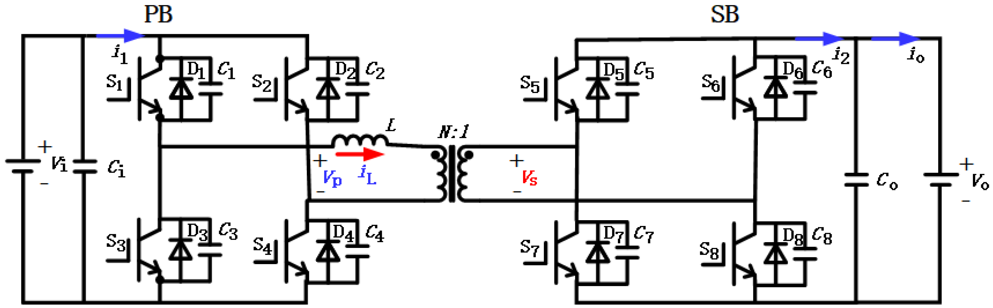
2. Mathematical Model of DAB Converter

The topology structure of the DAB converter is shown in Figure 1. The primary bridge (PB) and the secondary bridge (SB) are composed of switch transistors ( S 1 S 8 ), anti-parallel diodes ( D 1 D 8 ), and capacitors ( C 1 C 8 ). An equivalent leakage inductance L and a transformer connect the primary and secondary sides. In the topology, V i represents the input voltage, V o represents the output voltage, C i represents the input capacitance, C o represents the output capacitance, N:1 represents the transformer turns ratio, V p represents the voltage on the primary side, V s represents the voltage on the secondary side, i L represents the leakage inductance current, i 1 represents the input current, i 2 represents the output current, i o represents the load current, d represents the phase-shift duty cycle in single-phase modulation, and T s represents the switching period of the converter.
The average power transfer from PB to SB in the DAB converter can be expressed as:
P = N V o V i d 1 d 2 L f s
Assuming d > 0 and neglecting power losses in the switches and transformer, the output power must be equal to the input power, P o = P i . According to Equation (1), the output current i 2 can be expressed as [22]:
i 2 = N V i d 1 d 2 L f s
Based on Kirchhoff’s voltage law, the dynamic average model of the DAB can be represented as:
C o d V o d t = N V i d 1 d 2 L f s 1 R o V o
where R o represents the output load. This dynamic average model exhibits high accuracy, simplicity, strong verifiability, and scalability, making it widely used in the analysis and optimization of DAB control strategies in subsequent circuit simulations and designs. Since all these dynamic variables include DC components and small-signal AC components, these variables can be expressed as:
i 2 = I ¯ 2 + i ˜ 2 V i = V ¯ i + v ˜ i V o = V ¯ o + v ˜ o d = D ¯ + d ˜  
where I ¯ 2 ,   V ¯ i , V ¯ o , D ¯ represent the DC components of the output current, input voltage, output voltage, and duty cycle, respectively, while i ˜ 2 , v ˜ i ,   v ˜ o , d ˜ represent the AC components of the output current, input voltage, output voltage, and duty cycle, respectively. By substituting the above equations into Equation (3), the small-signal model of the DAB can be derived as [23]:
i ˜ 2 = C o d v ˜ o d t + 1 R o v ˜ o = N V ¯ i 1 2 D ¯ 2 f s L d ˜ + N D ¯ 1 D ¯ 2 f s L v ˜ i
Using Laplace transform, the transfer functions of the DAB system can be obtained as [24]:
G i 2 d = N V ¯ i 1 2 D ¯ 2 f s L G i 2 V i = N D ¯ 1 D ¯ 2 f s L G V o d = R o 1 + C o R o s G i 2 d

3. Controller Design and Genetic Algorithm Optimization Approach

Based on the DAB mathematical model presented in the previous section, this section provides a brief introduction to PI control based on the pole placement method, SMC and MPC. Additionally, it outlines the optimization approach of using GA for controlling parameter optimization.

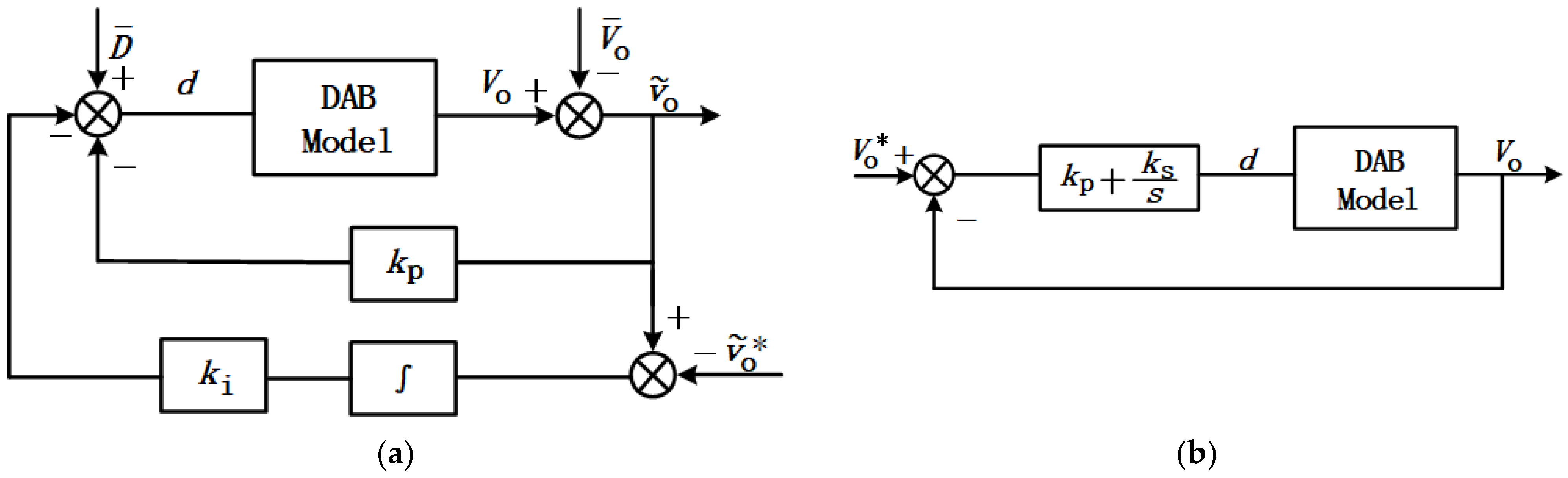
3.1. PI Control Based on Pole Placement Method

PI control is a classical control method that adjusts the controller output by comparing the error between the actual output and the desired output. In this article, a pole-placement-based PI control method is employed, which achieves control objectives by placing the poles at desired locations in the system. Specifically, based on the system model and desired performance requirements, the required pole positions are calculated and applied to the PI controller.
According to Equation (5), the small-signal model of the DAB can be expressed as:
d v ˜ o d t = 1 R o C o v ˜ o + N V ¯ i 1 2 D ¯ 2 f s L C o d ˜ + N D ¯ 1 D ¯ 2 f s L C o v ˜ i
Taking v ˜ o as the first state variable and 0 t v ˜ o v ˜ o * d t as the second state variable, where v ˜ o * represents the desired output voltage value, the state variables can be defined as:
X t = X 1 t X 2 t = v ˜ o 0 t v ˜ o v ˜ o * d t
The state equation is given by:
X ˙ t = 1 R o C o 0 1 0 X t + N V ¯ i 1 2 D ¯ 2 f s L C o 0 d ˜ + N D ¯ 1 D ¯ 2 f s L C o 0 v ˜ i + 0 1   v ˜ o *
Ignoring the terms v ˜ i and v ˜ o * , the above equation can be expressed as an open-loop state-space representation:
X ˙ t = A X t + B U t y t = C X t + D U t
where
A = 1 R o C o 0 1 0 , B = N V ¯ i 1 2 D ¯ 2 f s L C o 0 , C = 1 0 , D = 0
As shown in Figure 2, let the state feedback control be d ˜ = K X t , where K = k p k i and B 1 is the first component of input matrix B . Determine K such that the eigenvalues (poles) of the matrix A B K are placed at specified locations, which are also the roots of the characteristic polynomial of the matrix A B K :
det λ I A B K = λ 2 + 1 R o C o + B 1 k p λ + B 1 k i = λ 2 + 2 ξ ω n λ + ω n 2
where ξ is the damping coefficient of the second-order system, and ω n is the undamped natural frequency of the second-order system. ξ and ω n can be calculated based on the desired overshoot and peak time of the system using the following formulas:
δ = exp π ξ 1 ξ 2 t p = π ω n 1 ξ 2                      
where δ represents the overshoot of the second-order system, and t p represents the peak time of the second-order system. By solving the characteristic polynomial and placing the poles at the locations determined by the desired overshoot and peak time of the second-order system, the coefficients of the feedback control can be obtained as:
k p = 2 ξ ω n 1 R o C o B 1 k i = ω n 2 B 1                                        

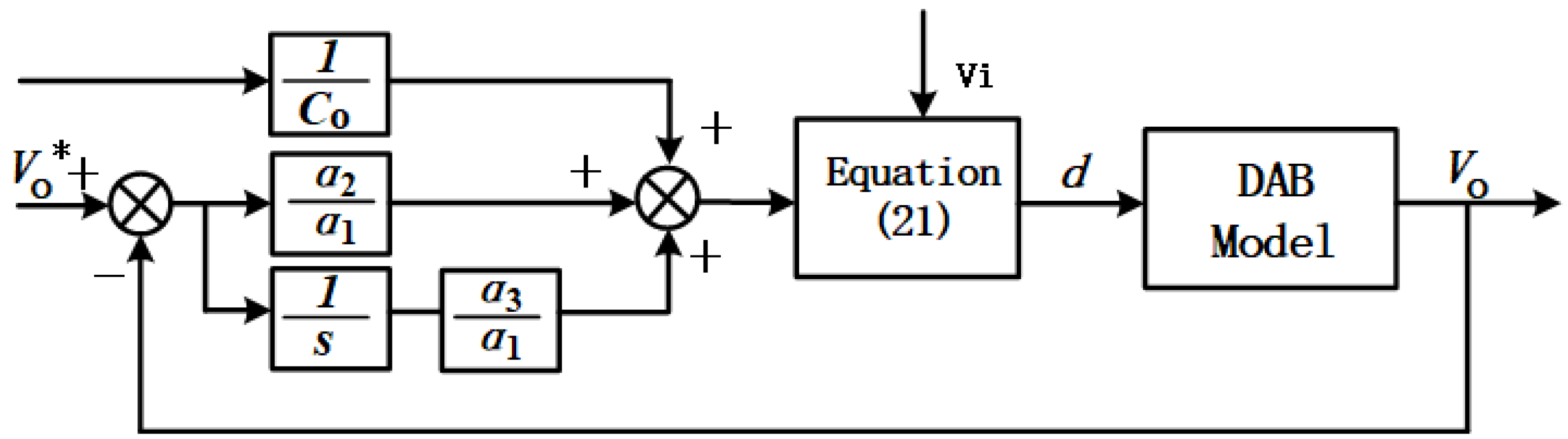
3.2. Sliding Mode Control

Due to the inability of the small-signal model to predict the stability of the converter under large transients, other control approaches need to be considered. SMC has many advantages as a control method. Firstly, SMC provides guaranteed stability and robustness against parameter uncertainties [22]. Secondly, SMC is a nonlinear control method that introduces the sliding mode to compensate for the system’s nonlinear characteristics and effectively handles stability issues during large transients. Therefore, adopting SMC is highly beneficial in ensuring the stability and robustness of the system in practical applications. In the DAB, a sliding mode can be introduced to control the output of the bidirectional transformer and full-bridge topology. This paper adopts a super sliding mode-based SMC approach, where the sliding mode is composed of the error between the system output and the desired output, as well as the rate of change of the error. Specifically, based on the system model and desired performance requirements, the required super sliding mode parameters are calculated and applied to the controller.
Firstly, the error between the output voltage and the reference voltage is selected as x 1 = V err = V o * V o , along with its integral as the state variable of the sliding surface. To eliminate the steady-state error introduced by the equivalent SMC, the quadratic integral of the aforementioned error is further chosen to eliminate the steady-state error. Therefore, the state variables of SMC are defined as:
x = x 1 x 2 x 3 T = V err 0 t V err   d t 0 t x 2   d t
The sliding surface represents the instantaneous feedback tracking trajectory of the system, and a linear combination of the weighted values of the state variables is selected as the sliding surface:
S x , t = i = 1 3 α i x i
where α i denotes the weighting coefficients of the sliding surface. Setting the first derivative of the sliding surface to zero ensures that the system state slides quickly on the sliding surface. In SMC, the direction of the control force is determined by the first derivative of the sliding surface, thus setting it to zero eliminates interference from the control force, ensuring that the system state slides quickly along the normal direction of the sliding surface, achieving fast and stable control effects. Using the invariance condition [25]:
d S x , t d t = 0
The equivalent control can be achieved, and based on Equation (15), we have:
i 2 = C o d V o d t + V o R o = V o R o + C o α 2 α 1 V err + C o α 3 α 1 0 t V err   d t
Secondly, setting the second derivative of the sliding surface to zero ensures that the control force has good robustness and adaptability. In SMC, due to uncertainties and disturbances affecting the system, the first derivative of the sliding surface will vary, thereby affecting the magnitude and direction of the control force. To maintain the stability and robustness of the control force, it is necessary to set the second derivative of the sliding surface to zero, which ensures that the control force has an appropriate adjustment speed and range when regulating on the sliding surface, avoiding excessive or insufficient adjustments that lead to system instability. Thus, we can set the second derivative of the sliding surface to zero [26],
d 2 S x , t d t 2 = 0
which leads to:
d 2 V o d t 2 + α 2 α 1 d V o d t + α 3 α 1 V o α 3 α 1 V o * = 0
The dynamics are designed as a critically damped second-order response, so the coefficients are chosen as:
α 2 α 1 = 2 ξ ω n α 3 α 1 = ω n 2          
where ξ represents the damping coefficient of the second-order system, and ω n represents the undamped natural frequency of the second-order system. ξ and ω n can be calculated based on the desired overshoot and peak time of the system. According to Equations (3)–(5), the static value of the phase-shift duty cycle can be expressed as:
d = 1 2 1 4 2 f s L i 2 N V i                 i 2 0 1 2 + 1 4 + 2 f s L i 2 N V i         i 2 < 0
Based on the above equations, the control block diagram of sliding mode control can be obtained as shown in Figure 3.

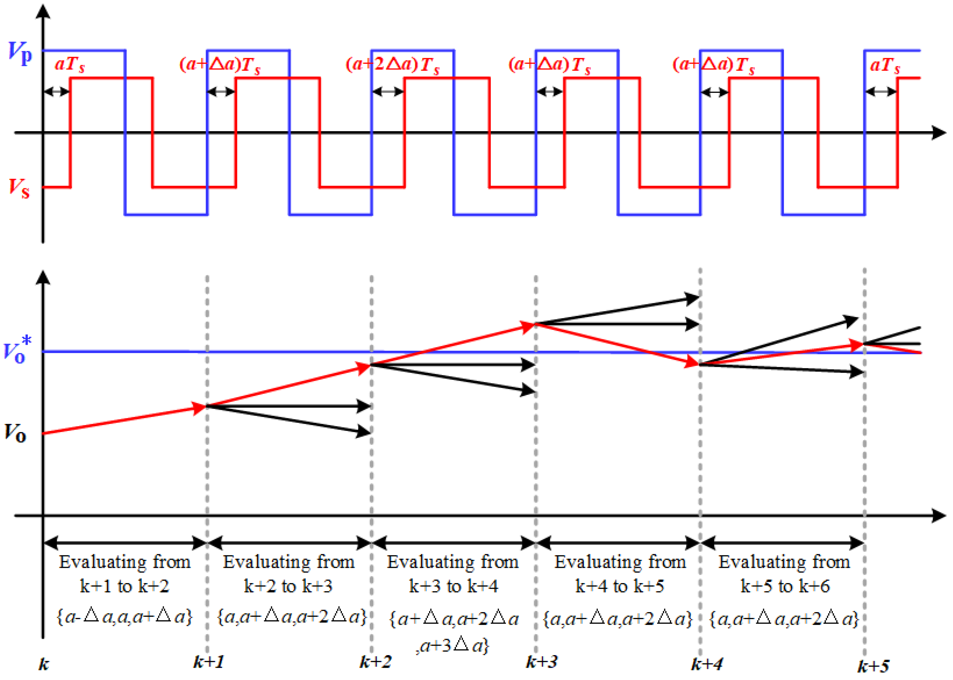
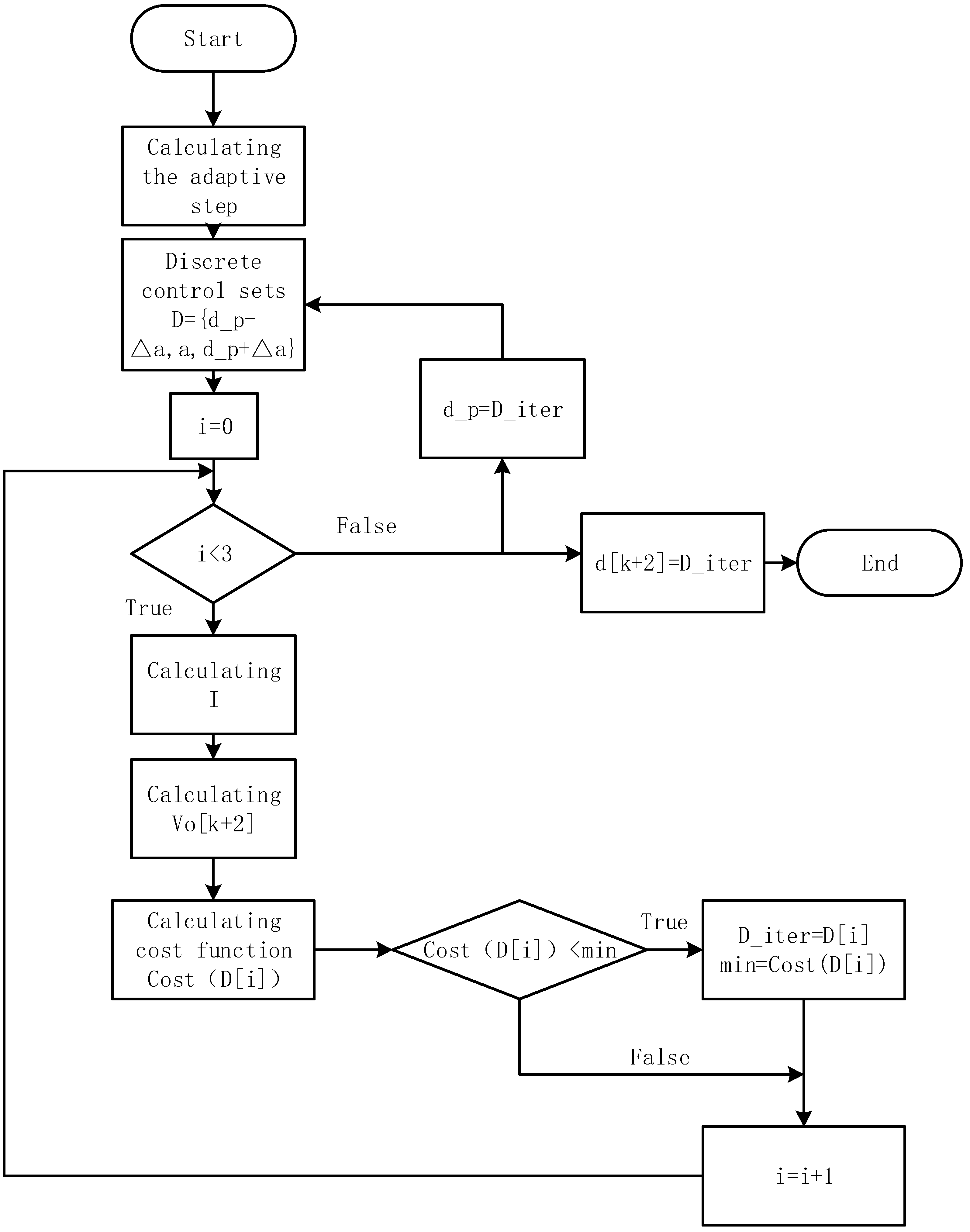
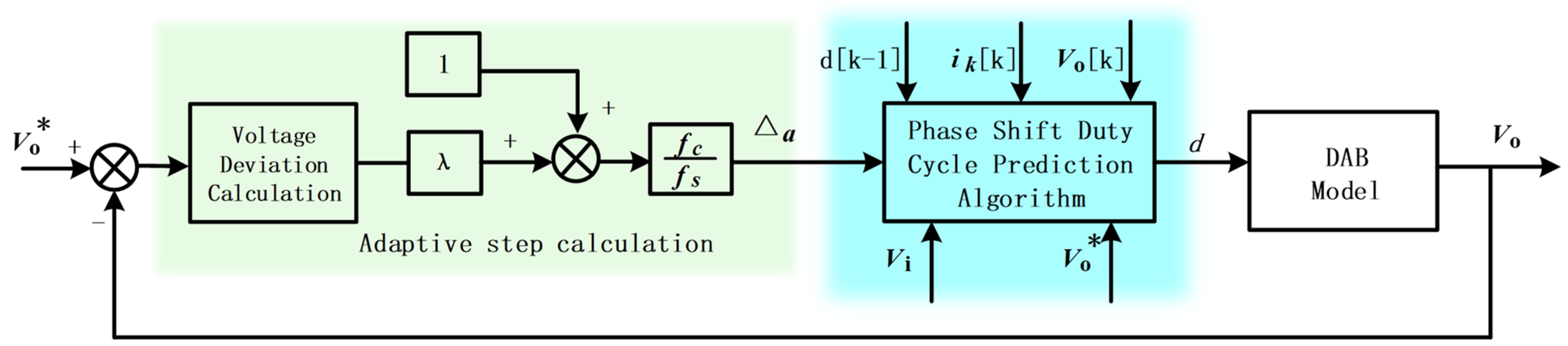
3.3. Model Preedictive Control

MPC is a model predictive control method that calculates control inputs by predicting the future states of the system and updates the control inputs at each sampling instant. Specifically, MPC models the system as a discrete-time dynamic model and uses this model to predict the future system states. Then, based on these predictions, an optimization problem is solved to determine the optimal control inputs that drive the system states towards the desired target states within a future time horizon.
According to Equation (3), we have:
C o d V o d t = i 2 i o
Using forward approximation, we can obtain:
V o k + 1 = i 2 k i o k C o f s + V o k
Assuming i o k = i o k + 1 , substituting Equation (23) into the output voltage at time step k + 2 , we can derive the discrete average model of DAB as:
V o k + 2 = V o k + i 2 k + 1 + i 2 k 2 i o k C o f s
Considering the cost function as [27]:
c o s t = α 1 G 1 + α 2 G 2
G 1 = V o * V o k + 2 2         G 2 = V o k + 2 V o k 2
G 1 and G 2 are two components in the controller. G 1 is responsible for regulating output voltage V o to the reference value V o * , while G 2 is responsible for reducing the voltage deviation. When V o deviates significantly from V o * , G 1 dominates the cost function. However, when V o approaches V o * , G 2 starts to play a role. G 2 limits the voltage variation, effectively suppressing the voltage ripple caused by analog-to-digital sampling noise and ensuring system stability [14].
Within one sampling period, three points are evaluated, centered around the previous operating point “a”, as shown in Figure 4.
f = f c / f s is defined as the finest achievable phase-shift value in the digital control platform, where f c is the peripheral clock of the microprocessor. The current discrete control set is d   ϵ   a f , a , a + f . The value a + f minimizes the cost function, and thus, it is used at time step k + 1 . The same overshooting is repeated in the next sampling period. An adaptive step size is employed instead of the minimum search step size f , defined as [28]:
V = V o * V o k ,         V o * V o k < V m   V m ,                                             V o * V o k > V m
a = f 1 + λ V
where V represents the voltage deviation, V m is the saturation voltage, and λ is a coefficient to be determined based on transient performance. Based on this adaptive step size, Figure 4 illustrates the working principle of DAB model predictive control. The next instant’s phase-shift duty cycle is calculated using the evaluation process shown in Figure 5, and this value is then transmitted to DAB for operation. The control block diagram of DAB model predictive control is depicted in Figure 6.

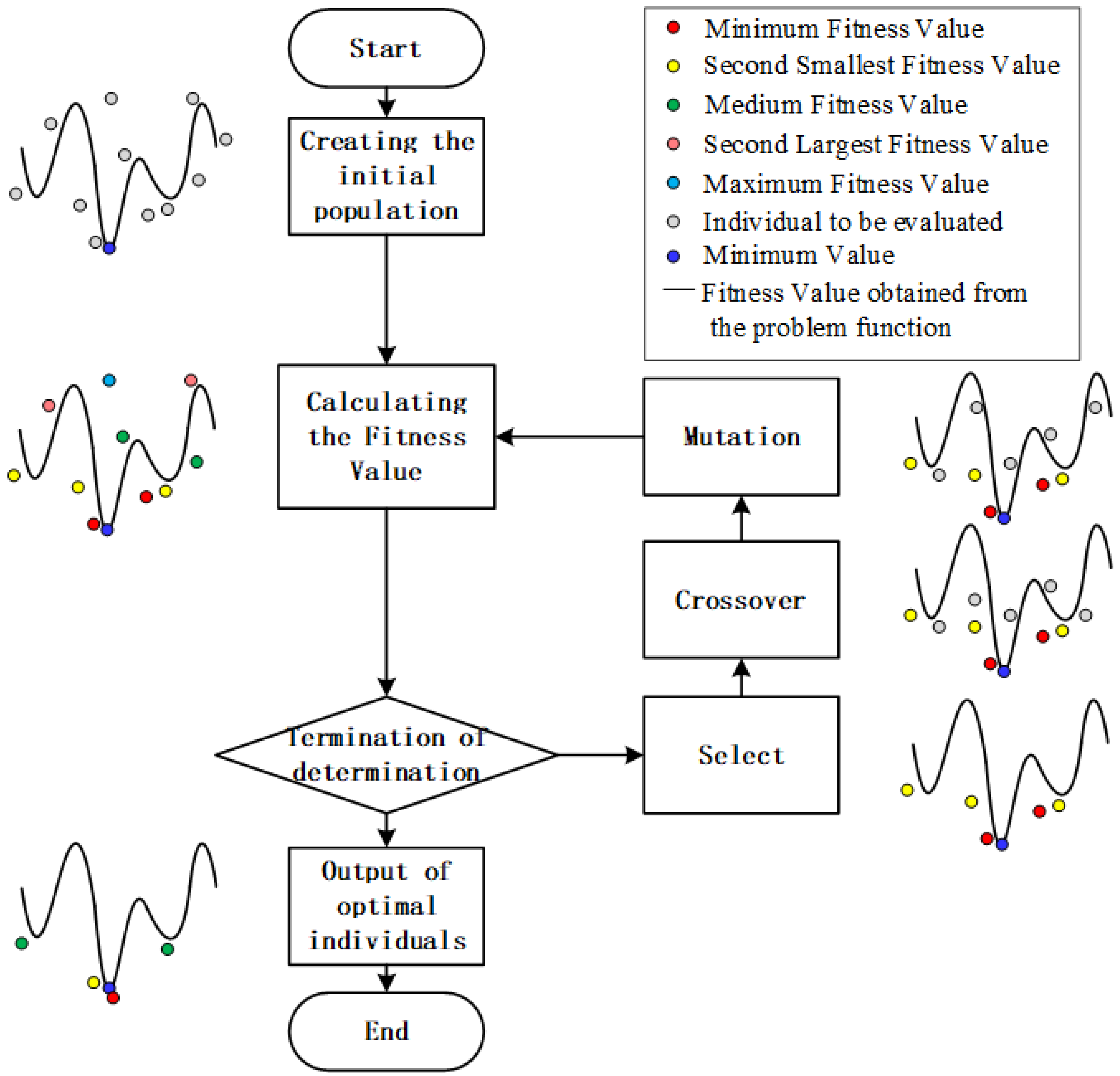
3.4. Genetic Algorithm

The selection of parameters in the DAB control method has a significant impact on the control performance and quality of the DAB system. While the PI control and SMC control can be adjusted and designed using expected peak time and overshoot, for MPC control, parameter selection relies on basic theory and experience. Therefore, choosing the appropriate control method and parameters for optimization becomes a key issue in improving the control performance and response speed of DAB. In this paper, GA is used to optimize the parameters of PI control, SMC control, and MPC control in DAB. By establishing the system model and control algorithms mentioned earlier, GA is applied for parameter tuning to optimize the control performance and response speed of DAB.
The concept of GA originates from evolutionary biology and is a random optimization search technique based on natural selection. The basic principle of the GA is to evolve better solutions by performing selection, crossover, and mutation operations on individuals (possible solutions) in the problem space. Each individual is represented as a chromosome, and the chromosome is composed of genes. Genes can be meaningful numerical values, symbols, or binary codes [21]. Figure 7 shows the flowchart of GA, while Algorithm 1 presents the pseudocode of GA, and its basic steps include the following.
1.
Population Initialization—Create an initial random population consisting of multiple individuals, with each individual corresponding to a potential solution. For the method of encoding the initial population, this paper defines the optimized variable range within lb and ub, and adopts real number encoding to encode the variables. Real number encoding is a common GA encoding method that transforms real-valued variables to gene values in the chromosome, where each gene represents a real-valued solution. In real number encoding, floating-point numbers are commonly used to represent gene values since the optimized variable range is usually a continuous real-valued range. Assuming the length of the chromosome is LC, each individual can be represented as an L C -length binary string or floating-point string. For real number encoding, the representation can be done using floating-point strings instead of binary strings. In real number encoding, it is necessary to perform the conversion between gene values and actual variable values to ensure that the optimized solutions fall within the variable range [29]. The detailed process of real-valued encoding is as follows:
(1)
Determine Chromosome Length—Initially, the length of the chromosome (number of genes) is established, which governs the encoding precision. Typically, this length depends on the number of problem variables and the required accuracy. Let us denote the chromosome length as L C ;
(2)
Initialize Individuals—For each individual, a random array of floating-point numbers is generated, with a length of L C . The range of each element (upper and lower limits) is set to 0 , 1 ;
(3)
Mapping Gene Values to Actual Variable Values—Transform each gene value into the range of the actual variable. Assuming the range of the variables to be optimized is m i n v a l ,   m a x v a l , the following formula is used to map the gene value genevalue to the actual variable value x : x = m i n v a l + g e n e v a l u e m a x v a l m i n v a l . Specifically, for each gene value genevalue, it is mapped to an actual variable value x, where x lies within the range m i n v a l ,   m a x v a l ;
2.
Evaluation of Fitness—Evaluate each individual in the population based on the problem’s objective function to obtain its fitness value, which measures the quality of the solution. In GA, the fitness function plays a crucial role in assessing the superiority of each individual. In this paper, the fitness function is defined as E r r o r = s u m V o * V o . Selecting this expression as the fitness function aims to choose control parameters with smaller voltage mutations during transient processes when operating conditions change, to better control the voltage stability of the DC bus;
3.
Selection—Based on the fitness values, select some individuals as “parents”, with the selection probability proportional to their fitness. In the selection operation, this paper adopts the elitism strategy. Elitism is a strategy that preserves the best individuals, passing the most excellent ones directly to the next generation in each population, ensuring the retention of excellent solutions [30]. This prevents the GA from losing the optimal solution during the optimization process. The individuals in the population are sorted from high to low based on the fitness values obtained in the previous step. The top few individuals with the highest fitness are selected as elite individuals and directly passed on to the next generation population;
4.
Crossover—Perform crossover operations on the selected parent individuals to generate new individuals (offspring) in the hope of obtaining better characteristics. This paper uses a random discrete crossover algorithm called crossoverscattered. It randomly selects two parent individuals and randomly chooses some gene positions for crossover. Then, it exchanges the selected genes at those positions between the two parent individuals, resulting in two offspring individuals [31];
5.
Mutation—Perform mutation operations on the offspring individuals, introducing random perturbations to maintain population diversity and explore new solution spaces [31]. This paper uses a uniform mutation algorithm called mutationuniform, which evaluates each gene in the individual based on the specified mutation probability. If the mutation probability requirement is met, the value of that gene is randomly perturbed within its range;
6.
Update Population—Combine the generated offspring individuals with the parent individuals to form a new population;
7.
Termination Criteria—Repeat the above steps until the predetermined termination criteria are met, such as reaching the maximum number of iterations or finding satisfactory solutions.
Algorithm 1: Genetic Algorithm
    Input: DAB parameters
                GA parameters
                GA options
    Output: the best control parameters of DAB
      // Initialize population using the “initializePopulation” function with population size “options.populationSize”.
1    population = initializePopulation(options.populationSize, numVars, lb, ub)
      // Evaluate fitness for each individual in the population using the “evaluateFitness” function.
2    evaluateFitness(population)
      // Sort the population based on fitness values.
3    sortPopulationByFitness(population)
      // Iterate over each generation.
4    FOR generation = 1 TO options.numGenerations
              // Initialize a new population to store the next generation.
5            newPopulation = []
              // Iterate over each individual.
6            FOR i = 1 TO options.populationSize
                      // Select parents using the “selectParent” function from the current popu lation.
7                    parent1 = selectParent(population)
8                    parent2 = selectParent(population)
                      // Generate offspring through crossover and mutation using the “crossover AndMutate” function, based on parents’ genes and within the bounds defined by “lb” and “ub”.
9                    child = crossoverAndMutate(parent1, parent2, lb, ub)
                      // Append the offspring to the new population.
10                   newPopulation.append(child)
11            END FOR
                // Update the population.
12            population = newPopulation
                // Reevaluate fitness and sort the population based on the updated fitness values.
13            evaluateFitness(population)
14            sortPopulationByFitness(population)
                // Retrieve the best individual.
15            bestIndividual = population [1]
16    END FOR
17    RETURN bestIndividual

4. Simulation Results and Performance Evaluation

Table 1 presents the circuit parameters of the DAB, while Table 2 provides specific values and the ranges for the parameters related to the GA used. In practical operating conditions, the DAB exhibits better performance in operating conditions involving reference tracking and load increase, while it shows relative difficulties in operating conditions with load decrease. Therefore, based on these parameters, a simulation circuit is constructed using MATLAB/SIMULINK. Against the background of a sudden decrease in load resistance from 20 Ω to 12 Ω (t = 0.1 s), the control parameters of PI control, SMC control, and MPC control are optimized using the error between the actual output voltage and the desired value as the objective function.

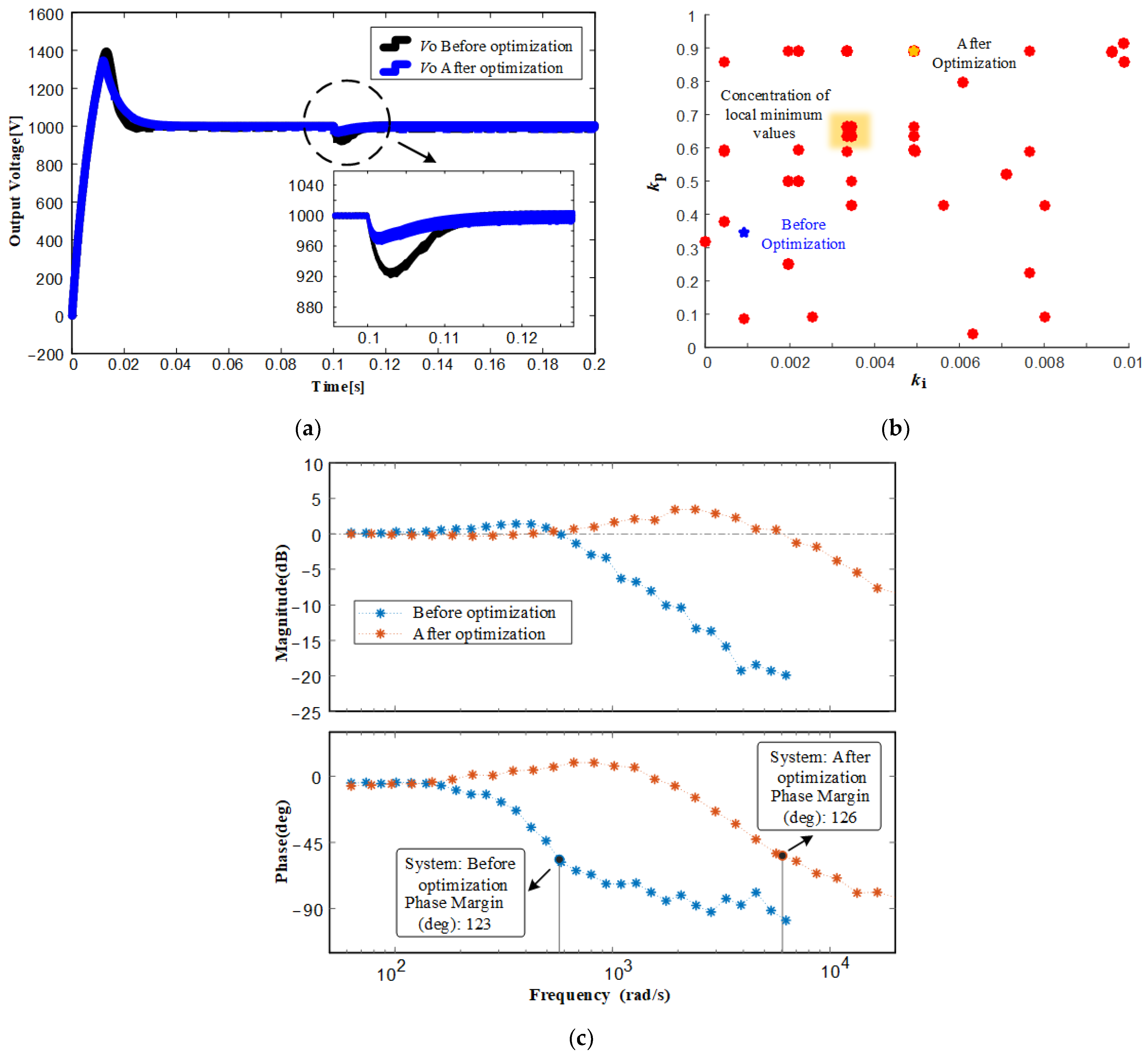
4.1. The Optimization Results of the Control Parameters for PI Control

GA is capable of effectively searching the parameter space and finding the optimal control parameters. For the PI control based on pole placement, setting an expected peak time of 10 ms and an expected overshoot of 5% can yield satisfactory control performance. The control parameters for the PI controller are selected to match these expected results: k i = 0.3453 and k p = 9.1459 × 10 4 . The optimized PI parameters obtained through GA are k i = 0.8908 and k p = 0.0049 . Figure 8 illustrates the optimization results for PI control parameters. Figure 8a shows the output voltage of the DAB. When the load suddenly decreases, the voltage drop value decreases from a maximum drop value of 920 V before optimization to 960 V after optimization, resulting in improved voltage stability.
Additionally, the maximum drop rate decreases from 8.00% to 4.00% after optimization, indicating better stability. Figure 8b illustrates the evolution of the parameters. It contains the pre-optimization and post-optimization parameter values. It is worth noting that there are some concentrated values of local minima in the figure. These values can be used to achieve different stability requirements in different cases of operating conditions variation.
The Frequency Response module in Simulink is used to perform frequency sweep on the closed-loop DAB system. Figure 8c presents the Bode diagram of the DAB system, showing an increase in phase margin from 123° (prior to optimization) to 126°, further enhancing system stability. A comparison with the parameters designed using the pole placement method reveals that the control performance of the GA-optimized control parameters is better.

4.2. The Optimization Results of the Control Parameters for SMC Control

Figure 9 presents the optimization results for SMC control parameters. For the SMC, aiming for an expected peak time of 10 ms and an expected overshoot of 5% leads to good control performance. The control parameters for the SMC controller are chosen to yield these expected outcomes: α 2 / α 1 = 599.1465 and α 3 / α 1 = 1.8844 × 10 5 . The optimized SMC control parameters obtained through GA are α 2 / α 1 = 1.6291 × 10 3 and α 3 / α 1 = 1.8410 × 10 5 .
Figure 9a illustrates the output voltage of the DAB, showing a reduced voltage drop from the pre-optimized maximum drop value of 925 V to 950 V after optimization. Moreover, the maximum drop rate decreases from 7.50% to 5.00% following optimization, signifying an improved stability. Figure 9c depicts the Bode diagram of the DAB system, showcasing an increase in phase margin from 127° to 155° after optimization, further highlighting the enhanced stability achieved by the optimized parameters.

4.3. The Optimization Results of the Control Parameters for MPC Control

Figure 10 displays the optimization results for MPC control parameters. In the case of MPC, the selection of weighting coefficients α 1 and α 2 influences the controller’s performance. A larger α 1 leads to quicker system response in bringing the output voltage close to the reference value, while a larger α 2 enhances the stability of maintaining the output voltage around the reference value. After multiple manual adjustments, the parameters α 1 = 100 and α 2 = 1 are chosen for comparison with subsequent optimization results. The optimized MPC control parameters obtained through GA are α 1 = 655.5732 and α 2 = 78.1755 .
Figure 10a illustrates the output voltage of the DAB, demonstrating a reduced voltage drop from the maximum drop value of 990 V to 993 V when the load suddenly decreases. Additionally, the maximum drop rate reduced from 1.00% to 0.70%, indicating an enhancement in stability. Figure 10c showcases the Bode diagram of the DAB system, with the gain margin increasing from 25.8 dB to 26.2 dB after optimization, further highlighting the enhanced stability achieved by the optimized parameters.
In summary, although the settling time slightly increases due to the reduced voltage drop, the use of GA to optimize the control parameters of the DAB results in improved control of the output voltage and reduced steady-state error. Therefore, GA exhibits great potential in optimizing controller parameters, effectively enhancing the performance and stability of control systems.

5. Discussion

The results obtained from the optimization of control parameters using GA for the DAB in different control strategies (PI control, SMC control, and MPC control) have shown significant improvements in control performance and system stability. The optimized controllers demonstrate reduced voltage drop and increased phase and gain margins, indicating better transient and steady-state responses under sudden load decrease conditions. These findings are crucial in enhancing the overall performance of the DAB in various practical operating conditions.
The optimized controllers’ improved performance, stability, and reduced steady-state error hold significant implications for the broader field of DC–DC converters and power electronics. The enhanced control of the DAB’s output voltage ensures reliable operation in practical scenarios with varying loads and disturbances. The application of GA in controller optimization can have a broad impact, not only in DABs but also in other power electronics systems, where precise control and stability are crucial.
Although the GA-optimized controllers demonstrate significant improvements, it is essential to acknowledge potential limitations. The optimized controllers’ performance may vary under extreme operating conditions or when facing highly nonlinear disturbances—for example, a shift in the direction of the DAB’s work or the input and removal of energy storage modules. Further investigations and robustness testing should be conducted to identify such scenarios and ensure the optimized controllers’ reliability in diverse situations. Meanwhile, the parameter tuning of GA can be challenging, requiring expertise and trial-and-error adjustments. Furthermore, the GA does not guarantee finding the global optimal solution, and may converge to local optima. Hence, in practical applications, it is essential to carefully tailor and refine the algorithm based on the problem’s characteristics and requirements. Particular attention should be given to the design of the fitness function, as it significantly influences the algorithm’s performance. By strategically addressing these concerns, one can enhance the effectiveness and efficiency of genetic algorithms for optimization tasks.

6. Conclusions

This paper introduces a novel metaheuristic algorithm-based control approach, namely, the method of optimizing the parameters of three typical DAB controllers using GA. The objective is to determine control parameters that enhance voltage stability, particularly under extreme operating conditions. Simulation results indicate that employing GA to optimize control parameters significantly reduces voltage drops in extreme conditions, reducing them by 40 V, 25 V, and 3 V for the three controllers, respectively. In comparison with pole-placement-based PI control and SMC control, the proposed GA optimization increases the phase margin by 3 degrees and 28 degrees, respectively. Compared to MPC control, the GA optimization enhances the gain margin by 0.4 dB. These results highlight the efficacy of GA optimization, with GA excelling in optimizing voltage drops for pole-placement-based PI control and significantly enhancing system stability for SMC control. Therefore, the utilization of GA for control parameter optimization greatly improves system stability, effectively addressing the limitations of traditional methods based on pole placement and manual parameter tuning. The optimized controllers demonstrate their potential ability to enhance the performance and stability of DC–DC converters. These findings have broader implications in the field of power electronics and offer valuable insights into the application of GA for controller optimization.

Author Contributions

Conceptualization, W.D. and W.C.; methodology, W.D.; software, W.D.; validation, W.D. and W.C.; formal analysis, W.D.; investigation, W.D.; data curation, W.D.; writing—original draft preparation, W.D.; writing—review and editing, W.C.; supervision, W.C. All authors have read and agreed to the published version of the manuscript.

Funding

This work was supported by the National Natural Science Foundation of China under Project 51977175.

Institutional Review Board Statement

Not applicable.

Informed Consent Statement

Not applicable.

Data Availability Statement

Data are available on request from corresponding author.

Conflicts of Interest

The authors declare no conflict of interest.

References

  1. Singh, S.; Gautam, A.R.; Fulwani, D. Constant power loads and their effects in DC distributed power systems: A review. Renew. Sustain. Energy Rev. 2017, 72, 407–421. [Google Scholar] [CrossRef]
  2. Lucas-Marcillo, K.E.; Guingla, D.A.P.; Barra, W.; De Medeiros, R.L.P.; Rocha, E.M.; Vaca-Benavides, D.A.; Orellana, S.J.R.; Muentes, E.V.H. Novel robust methodology for controller design aiming to ensure DC microgrid stability under CPL power variation. IEEE Access 2019, 7, 64206–64222. [Google Scholar] [CrossRef]
  3. Lucas, K.E.; Pagano, D.J.; Medeiros, R.L.P. Single Phase-Shift Control of DAB Converter using Robust Parametric Approach. In Proceedings of the 2019 IEEE 15th Brazilian Power Electronics Conference and 5th IEEE Southern Power Electronics Conference (COBEP/SPEC), Santos, Brazil, 1–4 December 2019; pp. 1–6. [Google Scholar]
  4. Jing, G.; Zhang, A.; Zhang, H. Review on DC Distribution Network Protection Technology with Distributed Power Supply. In Proceedings of the 2018 Chinese Automation Congress (CAC), Xi’an, China, 30 November–2 December 2018; pp. 3583–3586. [Google Scholar]
  5. Shao, S.; Chen, H.; Wu, X.; Zhang, J.; Sheng, K. Circulating Current and ZVS-on of a Dual Active Bridge DC-DC Converter: A Review. IEEE Access 2019, 7, 50561–50572. [Google Scholar] [CrossRef]
  6. Xia, P.; Shi, H.; Wen, H.; Bu, Q.; Hu, Y.; Yang, Y. Robust LMI-LQR Control for Dual-Active-Bridge DC–DC Converters With High Parameter Uncertainties. IEEE Trans. Transp. Electrif. 2020, 6, 131–145. [Google Scholar] [CrossRef]
  7. Li, K.; Yang, Y.; Tan, S.-C.; Hui, R.S.-Y. Sliding-mode-based direct power control of dual-active-bridge DC-DC converters. In Proceedings of the 2019 IEEE Applied Power Electronics Conference and Exposition (APEC), Anaheim, CA, USA, 17–21 March 2019; pp. 188–192. [Google Scholar]
  8. Zhang, L.; Wang, Y.; Cheng, L.; Kang, W. A Three-Parameter Adaptive Virtual DC Motor Control Strategy for a Dual Active Bridge DC–DC Converter. Electronics 2023, 12, 1412. [Google Scholar] [CrossRef]
  9. Shao, S.; Jiang, M.; Ye, W.; Li, Y.; Zhang, J.; Sheng, K. Optimal Phase-Shift Control to Minimize Reactive Power for a Dual Active Bridge DC–DC Converter. IEEE Trans. Power Electron. 2019, 34, 10193–10205. [Google Scholar] [CrossRef]
  10. Zhao, B.; Song, Q.; Liu, W.; Sun, Y. Overview of Dual-Active-Bridge Isolated Bidirectional DC–DC Converter for High-Frequency-Link Power-Conversion System. IEEE Trans. Power Electron. 2014, 29, 4091–4106. [Google Scholar] [CrossRef]
  11. Hebala, O.M.; Aboushady, A.A.; Ahmed, K.H.; Abdelsalam, I. Generic Closed-Loop Controller for Power Regulation in Dual Active Bridge DC–DC Converter With Current Stress Minimization. IEEE Trans. Ind. Electron. 2019, 66, 4468–4478. [Google Scholar] [CrossRef]
  12. Jeung, Y.C.; Lee, D.C. Voltage and Current Regulations of Bidirectional Isolated Dual-Active-Bridge DC–DC Converters Based on a Double-Integral Sliding Mode Control. IEEE Trans. Power Electron. 2019, 34, 6937–6946. [Google Scholar] [CrossRef]
  13. An, F.; Song, W.; Yu, B.; Yang, K. Model Predictive Control With Power Self-Balancing of the Output Parallel DAB DC–DC Converters in Power Electronic Traction Transformer. IEEE J. Emerg. Sel. Top. Power Electron. 2018, 6, 1806–1818. [Google Scholar] [CrossRef]
  14. Chen, L.; Shao, S.; Xiao, Q.; Tarisciotti, L.; Wheeler, P.W.; Dragičević, T. Model predictive control for dual-active-bridge converters supplying pulsed power loads in naval DC micro-grids. IEEE Trans. Power Electron. 2019, 35, 1957–1966. [Google Scholar] [CrossRef]
  15. Michalewicz, Z.; Schoenauer, M. Evolutionary algorithms for constrained parameter optimization problems. Evol. Comput. 1996, 4, 1–32. [Google Scholar] [CrossRef]
  16. Fleming, P.J.; Fonseca, C.M. Genetic Algorithms in Control Systems Engineering. IFAC Proc. Vol. 1993, 26, 605–612. [Google Scholar] [CrossRef]
  17. Meng, X.; Song, B. Fast Genetic Algorithms Used for PID Parameter Optimization. In Proceedings of the 2007 IEEE International Conference on Automation and Logistics, Jinan, China, 18–21 August 2007; pp. 2144–2148. [Google Scholar]
  18. Chahar, V.; Chhabra, J.; Kumar, D. Parameter Adaptive Harmony Search Algorithm for Unimodal and Multimodal Optimization Problems. J. Comput. Sci. 2013, 5, 144–155. [Google Scholar] [CrossRef]
  19. Richter, J.N.; Peak, D. Fuzzy evolutionary cellular automata. In Proceedings of the International Conference on Artificial Neural Networks in Engineering, Madrid, Spain, 28–30 August 2002; p. 185. [Google Scholar]
  20. Pilat, M.; White, T. Using Genetic Algorithms to Optimize ACS-TSP. In Ant Algorithms, Proceedings of the Third International Workshop, ANTS 2002, Belgium, Brussels, 12–14 September 2002; Springer: Berlin/Heidelberg, Germany, 2002; Volume 2463, pp. 282–287. [Google Scholar]
  21. Azab, M.; Serrano-Fontova, A. Optimal Tuning of Fractional Order Controllers for Dual Active Bridge-Based DC Microgrid Including Voltage Stability Assessment. Electronics 2021, 10, 1109. [Google Scholar] [CrossRef]
  22. Jeung, Y.-C.; Choi, I.-C.; Lee, D.-C. Robust voltage control of dual active bridge DC-DC converters using sliding mode control. In Proceedings of the 2016 IEEE 8th International Power Electronics and Motion Control Conference (IPEMC-ECCE Asia), Hefei, China, 22–26 May 2016; pp. 629–634. [Google Scholar]
  23. Qin, H.; Kimball, J.W. Generalized average modeling of dual active bridge DC–DC converter. IEEE Trans. Power Electron. 2011, 27, 2078–2084. [Google Scholar]
  24. You, W.; Zedong, Z.; Yongdong, L. DAB-based PET in MVDC traction and shipboard applications with distribution and redundant control. J. Eng. 2019, 2019, 3209–3213. [Google Scholar] [CrossRef]
  25. Tan, S.-C.; Lai, Y.-M.; Tse, C.-K. Sliding Mode Control of Switching Power Converters: Techniques and Implementation; CRC Press: Boca Raton, FL, USA, 2018. [Google Scholar]
  26. Martinez-Salamero, L.; Calvente, J.; Giral, R.; Poveda, A.; Fossas, E. Analysis of a bidirectional coupled-inductor Cuk converter operating in sliding mode. IEEE Trans. Circuits Syst. I Fundam. Theory Appl. 1998, 45, 355–363. [Google Scholar] [CrossRef]
  27. Chen, L.; Gao, F.; Shen, K.; Wang, Z.; Tarisciotti, L.; Wheeler, P.; Dragičević, T. Predictive control based DC microgrid stabilization with the dual active bridge converter. IEEE Trans. Ind. Electron. 2020, 67, 8944–8956. [Google Scholar] [CrossRef]
  28. Nardoto, A.; Amorim, A.; Santana, N.; Bueno, E.; Encarnação, L.; Santos, W. Adaptive Model Predictive Control for DAB Converter Switching Losses Reduction. Energies 2022, 15, 6628. [Google Scholar] [CrossRef]
  29. Chang, W.-D. Nonlinear system identification and control using a real-coded genetic algorithm. Appl. Math. Model. 2007, 31, 541–550. [Google Scholar] [CrossRef]
  30. Costa, L.; Oliveira, P. An Elitist Genetic Algorithm for Multiobjective Optimization. In Metaheuristics: Computer Decision-Making. Applied Optimization; Springer: Boston, MA, USA, 2003; Volume 86. [Google Scholar]
  31. Zainuddin, F.; Abd Samad, M.F. A Review of Crossover Methods and Problem Representation of Genetic Algorithm in Recent Engineering Applications. Int. J. Adv. Sci. Technol. 2020, 29, 759–769. [Google Scholar]
Figure 1. The topology structure of the DAB converter.
Applsci 13 10374 g001
Figure 2. Control block diagram of DAB PI control based on pole placement method: (a) DAB feedback control block diagram; (b) DAB feedback equivalent PI control block diagram.
Applsci 13 10374 g002
Figure 3. Control block diagram of DAB sliding mode control.
Applsci 13 10374 g003
Figure 4. DAB model predictive control working principle diagram.
Applsci 13 10374 g004
Figure 5. DAB model predictive control algorithm flowchart.
Applsci 13 10374 g005
Figure 6. Control block diagram of DAB model predictive control.
Applsci 13 10374 g006
Figure 7. The flowchart of the Genetic Algorithm.
Applsci 13 10374 g007
Figure 8. The optimization results for PI control parameters: (a) The output voltage of the DAB; (b) the evolution of control parameters; (c) Bode diagram of the closed-loop system with pre- and post-optimized control parameters.
Applsci 13 10374 g008
Figure 9. The optimization results for SMC control parameters: (a) The output voltage of the DAB; (b) the evolution of control parameters; (c) Bode diagram of the closed-loop system with pre- and post-optimized control parameters.
Applsci 13 10374 g009
Figure 10. The optimization results for MPC control parameters: (a) The output voltage of the DAB; (b) the evolution of control parameters; (c) Bode diagram of the closed-loop system with pre- and post-optimized control parameters.
Applsci 13 10374 g010
Table 1. DAB circuit parameters.
ParameterValueParameterValue
Vi2500 VVo1000 V
P50 kWfS10 kHz
o20 ΩN2.5
L8 × 10−4 HCo5 × 10−4 F
Ci5 × 10−5 Ftmax *2 × 10⁻⁶ s
* Maximum dead time of switching devices in DAB.
Table 2. Parameters of Genetic Algorithm.
ParameterValue
Population size20
The maximum number of generations50
Crossover probability0.8
Mutation probability0.01
The Number of elite individuals2
PI Control parameter
optimization boundary
k i 0 , 0.1 ; k p 0 , 1
SMC Control parameter
optimization boundary
α 2 / α 1 0 , 2000 ; α 3 / α 1 0 , 1 × 10 6
MPC Control parameter
optimization boundary
α 1 0 , 1000 ; α 2 0 , 1000
Disclaimer/Publisher’s Note: The statements, opinions and data contained in all publications are solely those of the individual author(s) and contributor(s) and not of MDPI and/or the editor(s). MDPI and/or the editor(s) disclaim responsibility for any injury to people or property resulting from any ideas, methods, instructions or products referred to in the content.

