Featured Application
This work applies machine learning, specifically LSTM and LSTM-NN models, to predict the Duffing equation’s convergence outcomes. It has potential applications in predicting vibration patterns in real-world systems like aircraft wings or automobile components to prevent adverse effects.
Abstract
This study addresses the problem of predicting convergence outcomes in the Duffing equation, a nonlinear second-order differential equation. The Duffing equation exhibits intriguing behavior in both undamped free vibration and forced vibration with damping, making it a subject of significant interest. In undamped free vibration, the convergence result oscillates randomly between 1 and −1, contingent upon initial conditions. For forced vibration with damping, multiple variables, including initial conditions and external forces, influence the vibration patterns, leading to diverse outcomes. To tackle this complex problem, we employ the fourth-order Runge–Kutta method to gather convergence results for both scenarios. Our approach leverages machine learning techniques, specifically the Long Short-Term Memory (LSTM) model and the LSTM-Neural Network (LSTM-NN) hybrid model. The LSTM-NN model, featuring additional hidden layers of neurons, offers enhanced predictive capabilities, achieving an impressive 98% accuracy on binary datasets. However, when predicting multiple solutions, the traditional LSTM method excels. The research encompasses three critical stages: data preprocessing, model training, and verification. Our findings demonstrate that while the LSTM-NN model performs exceptionally well in predicting binary outcomes, the LSTM model surpasses it in predicting multiple solutions.
1. Introduction
The Duffing equation is a significant nonlinear second-order differential equation commonly employed to model general oscillations in nonlinear systems. This equation captures various nonlinear vibration phenomena, including those that arise in circuits with specific inductance and capacitance configurations when subjected to electric current. It also describes dynamic friction effects, such as in oscillator systems, where nonlinearity leads to divergent behavior from linear systems at large vibration amplitudes. Furthermore, the Duffing equation finds application in analyzing vibrations in aircraft wings and automobiles, which, if severe, may cause damage to machine components. Therefore, estimating and understanding the vibration conditions is crucial for preventing potential harm. Among the studies related to the Duffing equation, Feng [1] employed the variational method and the theoretical approach of Dimensional Analysis to derive a novel analytical frequency function. This analytical function accurately describes the vibration frequency of the undamped Duffing equation. The validity and effectiveness of this frequency solution were confirmed through numerical simulations and experiments, providing a deeper understanding of the oscillation characteristics of the Duffing equation without damping. In another study, Rao [2] investigated the behavior of the Duffing equation in undamped free vibration and damped forced vibration scenarios. For undamped free vibration, Rao explained that varying initial conditions lead to the convergence results switching between 1 and −1 within a specific interval, exhibiting irregular changes. In the case of damped forced vibration, when specific initial conditions are fixed, the solution of the Duffing equation demonstrates various convergence patterns, such as single-cycle, double-cycle, and four-cycle, among others. Akhmet et al. [3] studied the bifurcation behavior of a Duffing oscillator in damped forced vibration, and used a bifurcation diagram and Lyapunov exponent to analyze the chaotic phenomenon of the system when the external force amplitude increased. Then, the Ott–Grebogi–Yorke (OGY) control method was used to stabilize the chaotic behavior and reduce its amplitude. They demonstrated the effectiveness of the OGY control method with numerical simulations, and confirmed that the types of multiple solutions in nonlinear equations have the potential to be studied. Therefore, this research is inspired to explore the types of various solutions of the Duffing equation. Compared with general analytical or numerical analysis, since the nonlinear solution takes a lot of computing time, this research will try to use machine learning to judge the value of multiple solutions of the Duffing equation.
Machine learning has experienced significant growth and has become widely utilized in various domains, leading to its rapid development in modern times. This powerful technology finds applications in diverse fields such as image recognition, search engines, industrial analysis, and artificial intelligence itself. The utilization of machine learning, along with the advancements in artificial intelligence, has shown substantial improvement in recent years, as indicated by statistics from Hao [4]. The trend of artificial intelligence application has evolved over time, progressing from the use of code command systems to the impact of machine learning and the widespread adoption of neural networks in the late 1990s and early 2000s. The continuous development of sophisticated algorithms and architectures, such as the three-layered model proposed by Hinton et al. [5], has paved the way for the progress of machine learning and artificial intelligence as a whole. In 2007, Hinton [6] introduced deep learning as an addition to the backpropagation method, enabling the adjustment of weights for improved training effectiveness. While this development brought significant advancements in weight updates and training, it did not fully address the issue of overfitting. To tackle this problem, Hinton et al. [7,8] proposed Dropout in 2012. This technique involves randomly dropping out neurons during the learning process, preventing excessive reliance on specific neurons and effectively mitigating overfitting. In 2015, Kingma et al. [9] presented the Adam optimizer, which combines the strengths of various previous optimizers. This method guides the training of each parameter in the loss function towards the most favorable direction, thus avoiding obstacles like saddle points and enhancing training speed and accuracy significantly. Furthermore, in 2018, Potdar et al. [10] conducted a study evaluating six different encoding techniques across six diverse datasets. These techniques included binary encoding, label encoding, and One-Hot Encoding, among others. The performance of each technique was assessed based on classification accuracy, and the impact of dataset size and the number of categories on each technique’s performance was analyzed.
In 1995, Mathia et al. [11] used multilayer perceptron (MLP) and Hopfield Neural Network (HNN) to find approximate solutions to approximate nonlinear equations by means of forward propagation. Predictions were made by a Recurrent Neural Networks (RNN) model. Not only has there been a great breakthrough in finding approximate solutions to nonlinear equations, but also the method of supervised learning has made great contributions to the prediction of nonlinear solutions. This also strengthens the confidence of using machine learning to analyze the solution of the Duffing equation in this study. Hochreiter and Schmidhuber [12] proposed the Long Short-Term Memory (LSTM) method. They improved RNN and improved the short-term memory ability of the original RNN to be able to deal with long-term and short-term memory problems. It not only improves the training speed, but also solves more complex and long-term dependent problems. In the area of high-dimensional partial differential equations, Han et al. [13] proposed a new method for solving high-dimensional partial differential equations (PDEs) using Deep Neural Networks. In the study of Wang et al. [14], the flutter speed was analyzed by the K-method, and the deep learning method of machine learning was used to predict the occurrence of flutter. They compared the performance of DNN and LSTM methods for flutter speed prediction, and attempted to predict aeroelastic phenomena in various flight conditions. Gawlikowski et al. [15] first gave an overview of various sources of uncertainty in deep learning, including data noise, model error, and model structure uncertainty. Applications of uncertainty estimation to deep learning were also discussed, including applications to active learning, decision making, etc. Hua et al. [16] used time series forecasting in fields such as finance, weather forecasting and traffic forecasting. They highlighted the potential of LSTM networks for time series forecasting and provided insights into the design and optimization of LSTM networks for their task. Hwang et al. [17] proposed a method called Single Stream RNN (SS-RNN). SS-RNN achieves single-stream parallelization by using a single GPU stream at each time step to process multiple sequences. They also proposed a method called Blockwise Inference for efficiently performing inference of RNNs on GPUs. In addition, Zheng et al. [18] proposed a compiler called Echo, which aims to reduce GPU memory usage during LSTM RNN training. Echo also provides an optimization method based on calculation graphs to reduce the number of data transmissions. Tariq et al. [19] proposed a method using multivariate convolutional LSTM (MC-LSTM) and mixed probabilistic principal component analysis (MPPCA) to detect anomalies in spatiotemporal data collected from space. This method was based on the LSTM model, and by adding convolutional layers, spatial and temporal features can be extracted from spatiotemporal data. Memarzadeh and Keynia [20] proposed a short-term electricity load and price forecasting algorithm based on LSTM-Neural Network (LSTM-NN). That algorithm was based on the combination of LSTM and Neural Network, and improved the prediction performance by optimizing the parameters of LSTM and Neural Network. He and El-Dib [21] discussed the Homotopy Perturbation Method (HPM) for nonlinear vibrations, focusing on challenges like non-conservative oscillators. It highlights key categories, provides heuristic examples, and the authors’ previous work on HPM. They concentrated on the Homotopy Perturbation Method (HPM) and its applications in solving nonlinear vibration problems, including non-conservative oscillators. Wang and Si [22] explored vibration phenomena in nanophysics using an efficient method based on ancient Chinese algorithms. It accurately determines amplitude–frequency relationships, offering valuable insights for nanophysics research. Wang and Wang [23] introduced the gamma function method to solve nonlinear cubic-quintic Duffing oscillators in one step, demonstrating its simplicity and accuracy for small amplitude oscillations. Their works seem to be more mathematically oriented, concentrating on analytical techniques to tackle nonlinear vibration problems, rather than building a database of nonlinear numerical data for machine learning. In the era of digital twins (DT), Zayed et al. [24] presented an AI-based fault diagnosis framework for industrial DT systems, including the triplex pump and transmission system. It combines optimization techniques with machine learning. Experimental results show FPA–CART and FPA–RF models maintain fault detection accuracy rates of 96.8% and 85.7%, outperforming other models in critical IIoT fields. Zhang et al. [25] introduced a digital twin-driven method for rolling bearing fault diagnosis in scenarios with limited training data. A virtual representation was created, and a Transformer-based network learned from it. Results demonstrated its effectiveness in real-world, unlabeled, and unknown health condition data. These works focused on fault diagnosis in industrial settings using digital twin-driven approaches, addressing scenarios where sufficient training data might be lacking.
The present work used Duffing equation to simulate the general nonlinear vibration situation and divided it into the special case of undamped free vibration and the condition of damped forced vibration. When the Duffing equation is in undamped free vibration, with the different initial conditions, the convergence result changes between 1 or −1 within a certain interval, and such changes are irregular. In addition, when the Duffing equation is in damped forced vibration, its solution will vary depending on the initial conditions, external forces, etc., and the final vibration condition will be different, and there may be multiple solutions. This study will observe the single-cycle convergent solution of the Duffing equation, especially the periodic solution of this system when the convergent trajectory is a single closed curve.
In order to collect the convergence results of the Duffing equation with two different types, this study uses the fourth-order Runge–Kutta method to collect the results of two different types, and changes the initial conditions and other parameters for analysis. Then, using the supervised learning method in machine learning, the undamped free vibration type is guided by the labeled method to guide the machine to analyze the target object cognitively. This study uses data preprocessing, training and validation to analyze the problem, and selects two algorithms to predict this nonlinear vibration phenomenon to analyze its accuracy. The two algorithms are: Deep Neural Networks (DNN) and Long Short-Term Memory model (LSTM). Among them, DNN is a supervised learning method, which is suitable for processing labeled data. LSTM is a branch of Recurrent Neural Networks (RNN) that solves the performance of time recurrent neural networks in long sequences and also solves the problems of gradient disappearance and gradient explosion, and is suitable for dealing with problems highly related to time series. Finally, use the Long Short-Term Memory model to add a small number of neuron hidden layers (LSTM-NN) to find the best learning model. This study aims to explore suitable learning models for predicting convergence results of nonlinear vibration equations in specific cases. To accomplish this, two different types of the Duffing equation will be examined as examples. The goal is to identify a learning model that can effectively predict the convergence outcomes of these nonlinear vibration equations.
The selection of the Long Short-Term Memory (LSTM) network structure in this proposed method is based on the unique characteristics of the problem we are addressing, which involve sequences and dependencies over time. LSTM is well-suited for dealing with sequential data, making it an ideal choice for time series analysis. In this study, we are working with time-dependent data from the Duffing equation, where each data point’s value depends on previous data points. LSTM was selected due to its proficiency in handling sequential data with long-range dependencies, which is crucial for modeling the intricate convergence patterns in the Duffing equation. Unlike traditional RNNs, LSTM mitigates the vanishing gradient problem, ensuring accurate predictions in time series analysis. LSTM’s memory cells further enhance its ability to capture complex temporal relationships, making it the optimal choice for our problem. We employ machine learning techniques, particularly LSTM and LSTM-NN models, to predict the convergence results of the Duffing equation. While Duffing equation studies exist, applying deep learning methods to this classical nonlinear differential equation is novel. We address two distinct scenarios: undamped free vibration and forced vibration with damping. These represent fundamental yet complex situations in nonlinear dynamics, and applying machine learning to predict their convergence outcomes is an innovative approach. Analytical comparison: We thoroughly explore the LSTM and LSTM-NN models, evaluating their performance in predicting both binary and multiple solutions. This in-depth analysis provides a novel perspective on the suitability of these models for specific types of data. Our research holds potential applications in various real-world systems, such as aircraft wings and automobile components, where nonlinear vibrations can occur. The practical implications of our findings contribute to the novelty of our work.
2. Theoretical Analysis
This study focuses on the Duffing equation, a representative nonlinear second-order differential equation commonly employed to simulate general nonlinear excited vibration systems. The equation describes various nonlinear vibration phenomena applicable to aircraft wing and automobile vibrations. Specifically, this research delves into the undamped free vibration type of the Duffing equation. When the linear and nonlinear elastic coefficients are identical, the solution converges to either +1 or −1. On the other hand, for the damped forced vibration type, the solution exhibits chaotic behavior in certain cases, while others converge to a limit cycle oscillation (LCO) result. For this situation, there is no analytical solution available so far. To address these phenomena, we numerically collect results for the +1 or −1 solutions in the undamped free vibration of the Duffing equation, along with the maximum and minimum displacements and velocities in the limit cycle oscillation of the damped forced vibration. Subsequently, we utilize deep learning methods to predict multiple solutions. In undamped free vibration of the Duffing equation, the convergence alternates between 1 and −1 based on the initial conditions. Conversely, in the presence of damping and external forces, the Duffing equation exhibits varying solutions, resulting in multiple outcomes. These convergent solutions lack regularity and defy analytical resolution. While numerical methods can approximate solutions, this irregularity presents an ideal testing ground for machine learning, specifically assessing the accuracy of the commonly employed LSTM method in addressing such complex scenarios.
The Duffing equation, a nonlinear second-order differential equation, finds applications in various fields, including: mechanical engineering, electrical engineering, aerospace engineering and materials science. The purpose of this article is to explore the accuracy of machine learning in analyzing classifying solutions of and limit cycle oscillation of the Duffing equation. This article focuses on two main themes: undamped free vibration and damped forced vibration. The characteristics of the undamped case include classifying solutions of , which can be applied in mechanical engineering for some simple vibrations, among other applications. The damped system, on the other hand, finds use in general civil and aerospace structural vibrations. This article does not consider multi-periodic solutions or chaos due to the limit cycle oscillation is already within the practical scope of engineering component design. Beyond this range, it is not typically applicable to general engineering design. Therefore, by considering these two scenarios, this article already covers most practical engineering applications. The Duffing equation, while widely employed, poses challenges due to its nonlinear nature, often lacking analytical solutions. This study aims to investigate two specific instances of the Duffing equation: one involves classifying solutions of , and the other concerns the quadruple solutions of limit cycle oscillation. These scenarios represent undamped and damped vibration conditions, holding significant practical utility.
2.1. Duffing Equation
Duffing equation can be written as follows:
where m is the mass, is the damping coefficient, and k and are the linear and nonlinear spring constant, respectively. is the external force, represents differentiation with respect to time, and is the vibration frequency. The undamped free vibration form of the Duffing equation is
Equation (2) can be divided into two forms, k > 0 and k < 0; when k < 0, the solution of Equation (2) contains two forms . However, when k > 0, Equation (2) can be obtained by “Dimensional Analysis method” to obtain a high-order approximate solution [1]. Once the analytical solution is obtained, it does not need to be estimated by machine learning methods for this case.
2.2. Numerical Solution of Fourth-Order Runge–Kutta Method
We use the fourth-order Runge–Kutta (RK-4) numerical method to solve the Duffing equation, and choose the coefficient of Equation (2) as k/m = /m = n:
In the case of changing different n, when the spring constants are equal, the displacement will happen to converge at two points, +1 or −1, and when n is different, the displacement convergence results are not the same, and there is no analytical solution, so it is worthy of further study. Figure 1 shows different initial displacements, initial velocities, and their convergence results for k/m = /m = 0.5. These results will be collected for subsequent analysis.
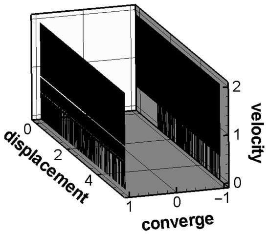
Figure 1.
Schematic diagram of the convergence results of the Duffing equation (undamped free vibration).
Then, we collect the data of the numerical solutions of the damped forced vibration type of the Duffing equation. This type will cause chaos under certain conditions. For example: m = 1, k = −1, , . The result is shown in Figure 2. In some cases, Limit Cycle Oscillation will appear, and its convergent trajectory is a single closed curve, for example: m = 1, k = 1, , . This solution corresponds to the periodic solution of the system, and forms a closed curve as shown in Figure 3. In addition, there are double loops or quadruple loops, etc. The trajectory of convergence is a closed curve composed of two cycles or four cycles. In this study, the fourth-order Runge–Kutta numerical method is used to collect data of different initial conditions, and only a single cycle solution is considered, and the maximum and minimum values of displacement and velocity of this closed curve will be recorded.
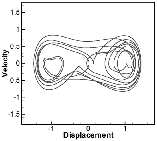
Figure 2.
The form of chaos in Duffing equation.
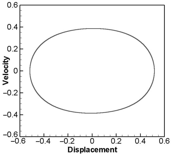
Figure 3.
Convergence graph of single limit cycle.
3. Deep Learning
3.1. Database Establishment
The chosen machine learning method for our study is supervised learning, which involves performing feature labeling actions on the data and input labels. Initially, we focus on the Duffing equation without damping and external force, as described in Equation (2). The initial conditions of this equation serve as data features, and we utilize the RK-4 method to calculate the convergence results of the equation. These results are then transformed into data labels using the One-Hot Encoding method, a widely-used tagging technique. Although the One-Hot Encoding method demands significant memory space and computation time, it provides substantial improvements in accuracy and an excellent training rate, particularly at lower values. The parameters utilized in our study include initial displacements and initial velocities. Table 1 presents the parameters and label data utilized in our database, which consists of a collection of 117,432 data sets.

Table 1.
The parameters and labels used in the Duffing equation (no damping).
The next step is to collect data on the single-cycle convergence results when the Duffing equation contains damping and external force terms. The parameters used are the initial displacements, initial velocities, natural vibration frequencies, damping coefficients, and external forces in Equation (1). In the process of collecting parameters, only single-cycle parameters and convergence data are kept, and the maximum and minimum displacements and velocities of single-cycle convergence results are used as prediction objects. Finally, 557,346 sets of data are collected as training and verification sets. Table 2 is the ranges of the parameters we chose, and Table 3 is the ranges of the results.
Table 2.
Parameters used in Duffing equation (damped forced vibration).
Table 3.
Convergence results of Duffing equation (damped forced vibration).
3.2. Deep Neural Network Architecture
Deep Neural Networks are the deeper Artificial Neural Networks (ANNs). The human brain can transmit and analyze information through the interconnection of neurons and make relative feedback. The neural network is composed of a large number of artificial neurons, and the artificial neurons are represented by Equation (4) and Figure 4.
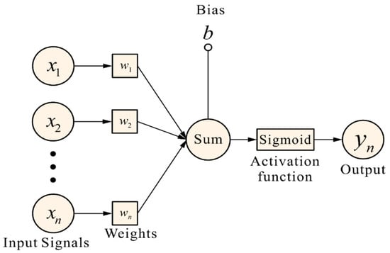
Figure 4.
Schematic diagram of artificial neuron.
Among them, x represents the value of neuron input, and w is the “weight”. Neurons and nearby neurons will influence each other, and the greater the weight, the greater the influence. If the weight of the input value is zero, any change of the current neuron has nothing to do with the output value. Therefore, different weight combinations will affect the overall output and then affect the overall accurate value. Additionally, the bias value (b), also known as Bias, introduces a deviation factor to the neural network, and is the activation function. After the input value has been processed by the weight value and deviation value, it needs to be transformed by an activation function (Activation Function). The activation function is used to transform the weighted sum of each input of the neuron to obtain the output signal. The architecture of Deep Neural Network is divided into three parts, namely input layer, output layer and hidden layer. There are multiple hidden layers between the input layer and the output layer. Each layer contains a plurality of neurons, which are, respectively, connected from the input layer to the hidden layer, and then, respectively, connected to the output layer from the hidden layer, as shown in Figure 5.
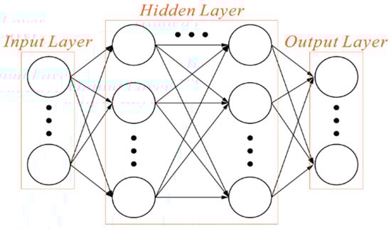
Figure 5.
Schematic diagram of Deep Neural Network.
Most of the algorithms in machine learning require a maximum or minimum function or index, which is called the object function, and the objective function of deep learning is usually a loss function. We choose categorical cross-entropy, which is more commonly used in classification problems, as the loss function of our Deep Neural Network architecture. The operation of categorical cross-entropy is shown in Equation (5).
Among them, ED refers to the loss function, while n represents the number of classification categories. The variable yi corresponds to the labeled data, and pi denotes the accuracy rate of the classifier in predicting the convergence result of the Duffing equation. When employing the classification cross-entropy loss function, the activation function for the output layer is selected as Softmax. The equations presented above correspond to the forward propagation phase, which can be visualized as a series of operations performed from left to right. The input passes through the weights and bias values, undergoes function transformations, and progresses until reaching the output. On the other hand, the backpropagation algorithm is a more efficient variant of the gradient descent method. It calculates the gradient by means of partial differentiation and adjusts the weights to minimize the error. By leveraging the chain rule, the backpropagation method combines the gradient descent approach and serves as an optimization algorithm. Notably, the backpropagation process is the reverse of the forward propagation. Equation (6) demonstrates that the backpropagation method employs the loss to compute the gradient of the loss function in each layer.
where y is the value of the weighted product transformed by the activation function.
3.3. The Basic Structure of LSTM
In the data preprocessing stage, we prepare the dataset by collecting convergence results of the Duffing equation for both undamped free vibration and damped forced vibration scenarios. These data are then carefully preprocessed to ensure their quality and suitability for training. We perform feature engineering and normalization to prepare the data for the machine learning models. For model training, we employ two primary algorithms: recurrent Neural Networks (RNN) and Long Short-Term Memory (LSTM) models. These models are used to predict the convergence outcomes of the Duffing equation for the specific cases we have explored. Regarding the loss function, we use Mean Squared Error (MSE) as our primary loss function during the training process. MSE measures the average squared difference between the predicted values and the actual convergence outcomes. Our goal is to minimize this loss function during training, which essentially means that our models aim to make predictions that are as close as possible to the real convergence results. This combination of data preprocessing, model selection (DNN and LSTM), and the MSE loss function allows us to effectively train our machine learning models to predict the complex convergence patterns of the Duffing equation in the specific scenarios we have studied.
A temporal recurrent neural network is a specific type of neural network that processes information sequentially in one direction. It possesses connections between hidden layers, known as recurrent connections, which enable the network to retain past information while incorporating new information. These connections allow for information to flow and facilitate short-term memory capabilities. Figure 6 illustrates the architecture of a temporal recurrent neural network. During the operation of the long-term short-term memory unit state, it undergoes calculations similar to a Deep Neural Network. It involves multiplying the input with a weight, adding a bias value, and subsequently updating the state using a control gate. The unit state and control gate are transformed using activation functions. In this case, the unit state employs a hyperbolic tangent function as its activation function, while the control gate employs a sigmoid function as its activation function.
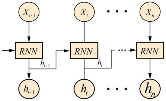
Figure 6.
Time Recurrent Neural Network architecture (LSTM).
In LSTM networks, an objective function is essential for training. Mean Square Error (MSE) is a commonly used loss function in regression problems. MSE calculates the average of the squared differences between the predicted values and the actual values. It focuses solely on the magnitude of the errors and disregards their direction, quantifying the error based on the deviation distance. Assuming there are q records, the calculation formula for MSE can be represented as Equation (7),
where yi is the actual value after labeling, and is the predicted result.
During the training process, the loss function is evaluated across the entire training set. However, to effectively minimize the loss function, it is crucial to employ an optimizer that guides the parameters in the right direction. Optimizers play a vital role in deep learning, as they enhance training efficiency, help avoid becoming stuck in saddle points, and mitigate overfitting issues. In this study, we refer to [8] and select the Adam optimizer for training purposes. The Adam optimizer combines the strengths of the Adagrad and Momentum optimizers. Adagrad adjusts the learning rate to improve training efficiency. Equation (8) represents the basic concept of the Adagrad algorithm.
In the equations, represents the weight, denotes the learning rate, g signifies the gradient of , Gt,ii is the sum of the squared gradients from previous steps, and ε is a smoothing term. The purpose of changing the learning rate using Gt is to address issues such as overfitting and slow training. Initially, with smaller values of Gt, a higher learning rate is employed, resulting in faster training efficiency. As Gt increases over time, the learning rate decreases to mitigate overfitting concerns. The smoothing term (ε) prevents the denominator from becoming zero. However, in cases where the Adagrad optimizer has a large value in later stages, the learning rate may become excessively low, resulting in slow training. On the other hand, the Momentum optimizer adjusts the learning rate based on the gradient direction. When the gradients align in the same direction, the learning rate gradually accelerates, whereas it decreases when the gradients are in the opposite direction. Equations (9) and (10) depict the concept of the Momentum algorithm.
If vt represents the previous term, it gradually grows larger, leading to an increase in the weight value. However, the Momentum method is unable to anticipate certain situations. If we have prior knowledge of the upcoming direction, we can make necessary preparations. The Adam (Adaptive Moment Estimation) optimizer combines the capability of the Momentum algorithm to adjust speed based on past gradient directions with the ability of the Adagrad algorithm to update the learning rate.
Equations (11) and (12) represent the Adam algorithm, which encompasses these combined functionalities.
Among them, both mt and vt require correction for deviation to prevent them from being initialized as zero vectors, which would cause them to gravitate towards zero. We utilize Equations (13) and (14) to calculate the bias correction and counteract any bias present.
After correcting Equations (13) and (14), the gradient update rule of the Adam algorithm is shown in Equation (15).
In parameter setting, the learning rate is set to 0.003, the default value of is 0.9, while is 0.999, and is 1 × 10⁻⁸. When selecting an activation function, different activation functions need to be selected according to different states. The activation functions we use for training include Simgoid function, Hyperbolic tangent function, Softmax function, etc. Sigmoid is a synthetic function of natural exponents, which can convert the input into a number between 0 and 1. Equation (16) is the mathematical definition of the Sigmoid function:
Hyperbolic tangent function is more commonly used in time-recurrent neural network architecture, and its value range is [−1, 1]. Equation (17) is the mathematical definition of Hyperbolic tangent function:
The Softmax function, as defined by Equation (18), ensures that its output falls within the interval [0, 1].
4. Deep Learning Training Analysis
4.1. Duffing Equation Undamped Free Vibration Type—By LSTM Model
We use the LSTM method to predict the convergence outcome of the undamped free vibration type of the Duffing equation. The dataset comprises a total of 117,432 records. Initially, we construct an LSTM framework capable of training these data and partition it into three sets. The training set consists of 65% of the total data, the validation set contains 30%, and the remaining 5% is allocated as the prediction set. The model’s input parameters consist of initial displacement, initial velocity, nonlinear and linear spring constants, while the output dataset consists of the convergence values of the equation’s solution. After establishing the fundamental structure of the LSTM model for data training, we utilize two hidden layers with 10 neurons each. We conduct 10,000 epochs with a batch size of 16,284. The training results are presented in Figure 7.
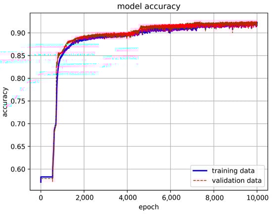
Figure 7.
The results of basic LSTM model training.
Once we employ the One-Hot Encoding technique to label the output, we can distinguish the output values across different dimensions. This method proves particularly effective when the output values are limited in range. In the case of the undamped free vibration mode of the Duffing equation, where only two convergence types (+1 or −1) exist, we find this approach suitable and employ it. To address concerns regarding overfitting, we incorporate dropout layers in each hidden layer. To determine the optimal configuration for the hidden layers, we conduct tests with varying numbers of layers. The accuracy and loss results for different hidden layer configurations are illustrated in Figure 8 and Figure 9, respectively.
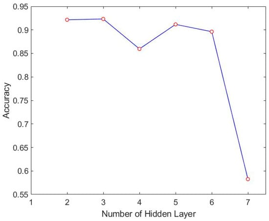
Figure 8.
Accuracy results of different hidden layers of LSTM.
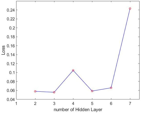
Figure 9.
Loss of different hidden layers of LSTM.
According to the accuracy and loss of LSTM method mentioned above, the best number of hidden layers can be found to be three. We then adjust the number of neurons to find the best result. The accuracy and loss of different numbers of neurons are shown in Figure 10 and Figure 11.
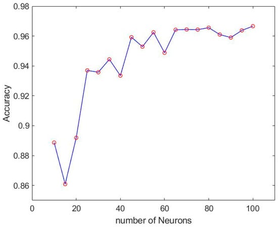
Figure 10.
Training results of different neurons of LSTM.
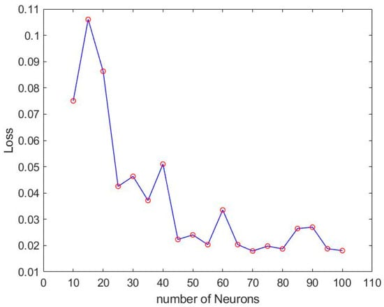
Figure 11.
Loss of different neurons of LSTM.
From Figure 12 of the training results, it can be concluded that when the number of neurons is 55, the training result has reached 96% accuracy, and the loss is only 2%. But it was also found that there will be instability when using LSTM. There are almost 5% unstable oscillations in the accuracy rate. The unstable situation is shown in Figure 13 and Figure 14.
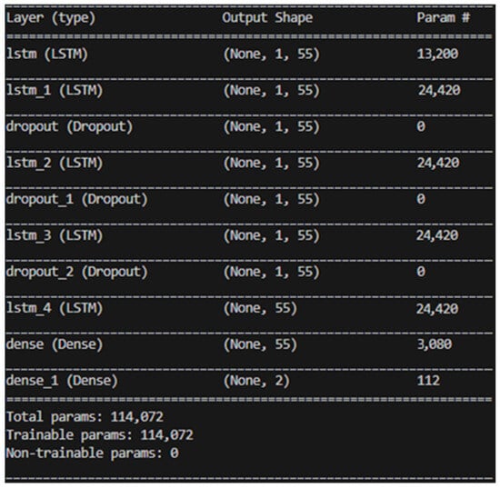
Figure 12.
LSTM best trained model.
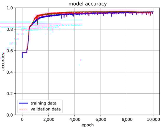
Figure 13.
The unstable situation of LSTM model accuracy.
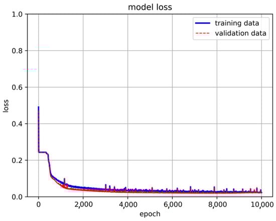
Figure 14.
The unstable situation of LSTM model loss.
4.2. Duffing Equation Undamped Free Vibration Type—By LSTM-NN Model
When training the LSTM model for the undamped free vibration type of the Duffing equation, it was observed that the accuracy rate after training exhibited instability. To address this issue and enhance the prediction results, we introduced deep neural network hidden layers while modifying the activation function. Using the same dataset, we initially established an LSTM framework capable of training these data. Following the approach described in Section 4.1, we divided the data into three parts: the Training set (comprising 65% of the total data), the Validation set (30%), and a separate 5% as the prediction set. The number of neurons was initially set to 30. Table 4 presents the accuracy and loss values for different hidden layers.
Table 4.
Accuracy and loss percentage of different hidden layers.
After evaluating the accuracy, loss, and stability of various architectures, this study ultimately adopts a model architecture consisting of three hidden layers of LSTM and two hidden layers of neural networks. Subsequently, adjustments were made to the activation function. Initially, we experimented with replacing the previously used ReLU function with the sigmoid function in search of the optimal learning model. However, the use of the sigmoid function did not yield better results. Consequently, the final model architecture for this research consists of three layers of LSTM hidden layers and two layers of neural network hidden layers, utilizing the ReLU activation function, as illustrated in Figure 15. The training results are presented in Figure 16 and Figure 17.
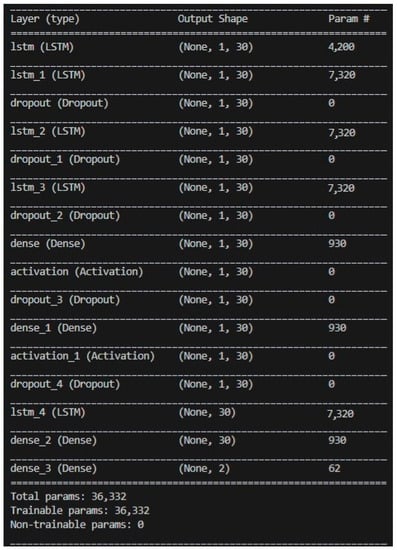
Figure 15.
LSTM-NN model architecture.
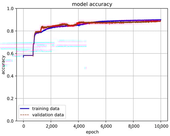
Figure 16.
The accuracy of the 3-LSTM hidden layer + 2-NN layer model.
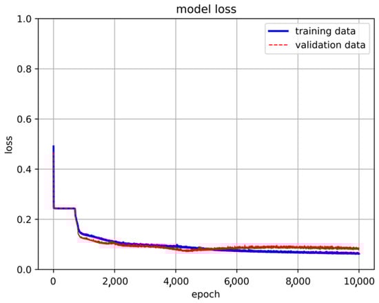
Figure 17.
The loss of the 3-LSTM hidden layer + 2-NN layer model.
After finding the best learning model architecture, we changed the number of neurons in each layer to find the best training model. The results after training are shown in Figure 18 and Figure 19.
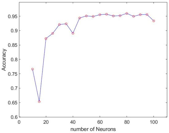
Figure 18.
The accuracy of LSTM-NN architecture with different numbers of neurons.
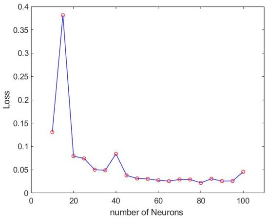
Figure 19.
The loss of LSTM-NN architecture with different numbers of neurons.
According to training accuracy, loss and stability among different neurons, the optimal number of neurons is 80. Its stability is significantly better than the model using only LSTM, and it has excellent performance in accuracy and loss. The accuracy of the training results is 96% and the loss is 2.1%, and the accuracy is unstable with only 1% fluctuation. The training model is shown in Figure 20 and the results are shown in Figure 21 and Figure 22.
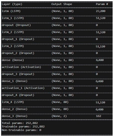
Figure 20.
LSTM-NN model architecture for final use.
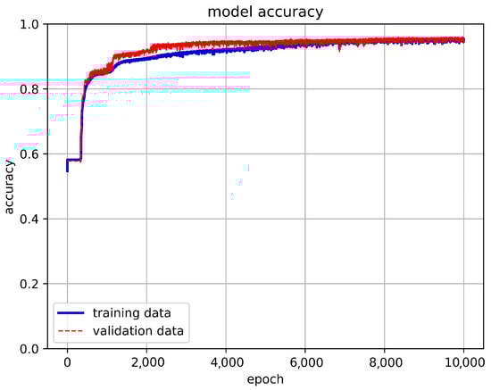
Figure 21.
The accuracy of the final training results of the LSTM-NN architecture.
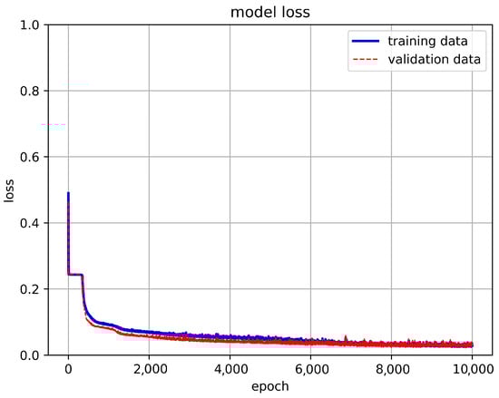
Figure 22.
The loss of the final training results of the LSTM-NN architecture.
4.3. Duffing Equation Damped and Forced Vibration Type—By LSTM Model
In this study, we apply the method described in Section 2 to gather convergence results of the damped forced vibration type of the Duffing equation. The dataset is created by collecting the maximum and minimum values of displacement and velocity from the convergence outcomes. These data are then split into a 65% training set, a 30% validation set, and the remaining 5% is used as the prediction set. The model’s input parameters consist of initial displacement, initial velocity, damping coefficient, natural vibration frequency, and external force. Initially, we train the model using 557,346 data values, employing a model architecture with one hidden layer comprising 80 neurons. We conduct 3000 epochs with a batch size of 16,384. However, we observe underfitting in the validation set, indicated by an upward trend in the loss around the 500th epoch. Figure 23 illustrates the training results. To tackle overfitting, we include a dropout layer during the training process. Additionally, unlike in Section 4.1, where the One-Hot Encoding method was used to label the target parameters, in the case of training multiple numerical solutions, we directly use the original values as labels to ensure the credibility of the target parameter predictions.
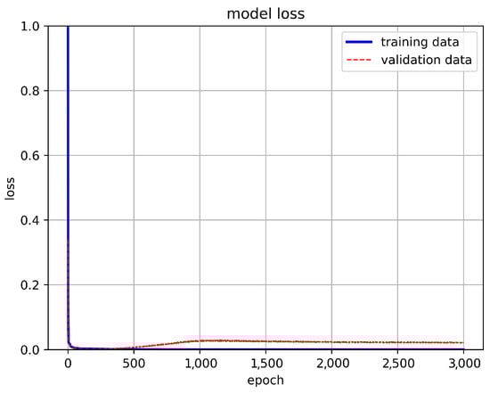
Figure 23.
Results of the first training.
According to the method in Section 4.1, we first adjust the number of different hidden layers to find out the training results of each layer. As shown in Figure 24 and Figure 25, it can be seen that when training to three hidden layers, better results can be obtained. Subsequent hidden layers with different numbers do not grow very well, and the training time is longer. So we choose three hidden layers as the architecture of the training model.
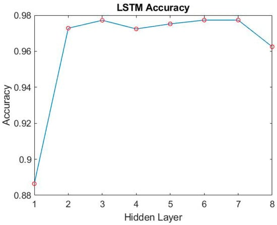
Figure 24.
The accuracy of different hidden layers of LSTM.
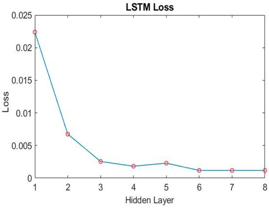
Figure 25.
The loss of different hidden layers of LSTM.
After establishing the LSTM training model, we proceed to fine-tune the number of neurons, exploring different configurations at intervals of every 10 neurons. The training results for various neuron counts are presented in Figure 26 and Figure 27. Notably, when utilizing 60 neurons, the model achieves exceptional performance with a minimal loss of only 0.17% and an outstanding accuracy rate of 97.5%. As a result, this study selects 60 neurons as the optimal number within the final LSTM model architecture, as illustrated in Figure 28.
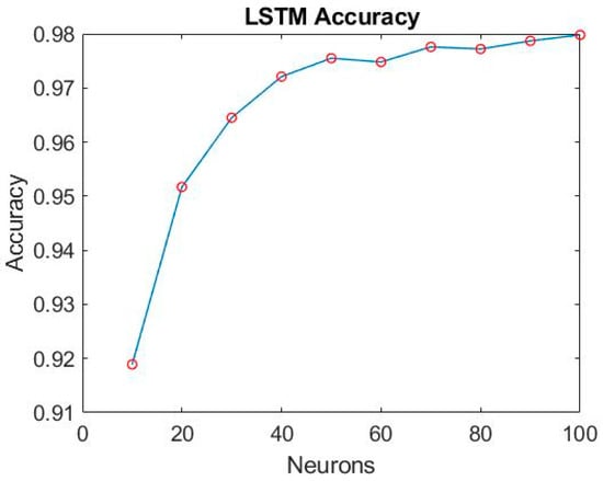
Figure 26.
The accuracy of LSTM with different numbers of neurons.
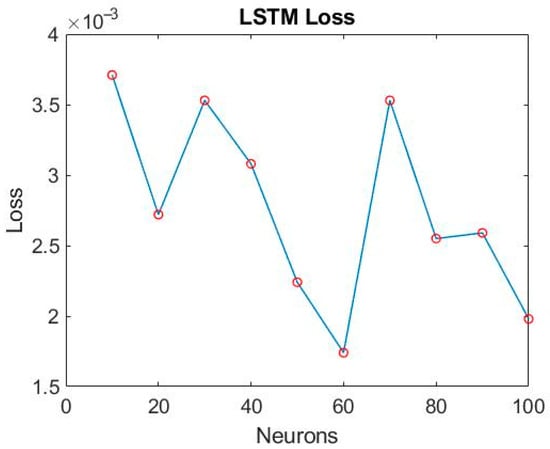
Figure 27.
The loss of LSTM with different numbers of neurons.
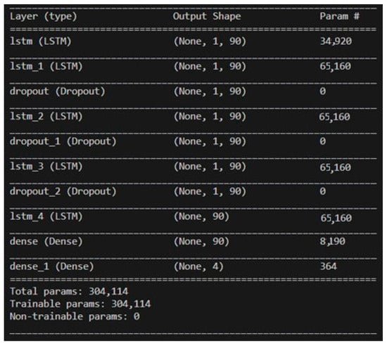
Figure 28.
LSTM model architecture for final use.
4.4. Duffing Equation Damped and Forced Vibration Type—By LSTM-NN Model
The dataset of 557,346 records was divided into approximately 65% for the training set, 30% for the validation set, and 5% for the prediction set. The model utilized 80 neurons, underwent 3000 epochs, and used a batch size of 16,384. The training method was based on the target parameters described in Section 4.2, where training and prediction employed the original values to ensure result credibility. Table 5 presents the training results for different hidden layers. Notably, when the LSTM hidden layer consisted of three layers combined with one neural network hidden layer utilizing the ReLU activation function, the model achieved an exceptional accuracy rate of 98.14% with a loss of 0.07%. Training accuracy and loss are depicted in Figure 29 and Figure 30, respectively.
Table 5.
Accuracy and loss percentage of different hidden layers.
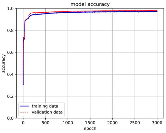
Figure 29.
LSTM-NN model training accuracy.
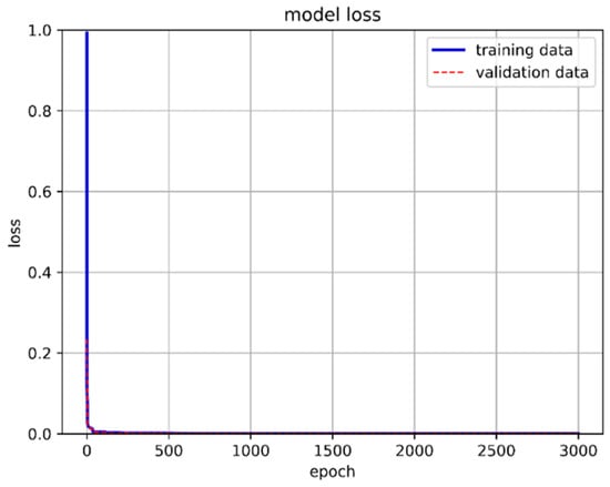
Figure 30.
LSTM-NN model training loss.
After choosing a model architecture for training, its number of hidden layer neurons is adjusted. We started with 10 neurons as the minimum number and increased by 10 units each time to 100. The epoch is adjusted to 5000 according to the downward trend of its loss, and its accuracy and loss are collected. Figure 31 and Figure 32 are the training results of different numbers of neurons.
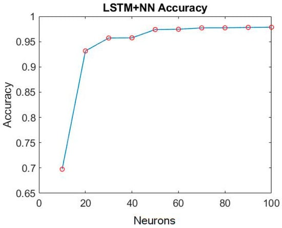
Figure 31.
The accuracy of LSTM-NN with different numbers of neurons.
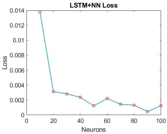
Figure 32.
The loss of LSTM-NN with different numbers of neurons.
When the number of neurons reaches more than 50, its training accuracy is as high as 97.5%. When the number of neurons is 90, the loss is only 0.046%. So, the number of hidden layer neurons in the final model architecture is set to 90. Figure 33 shows the final selected model architecture.
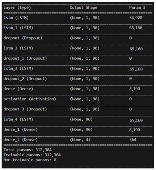
Figure 33.
LSTM-NN model architecture for final use.
5. Deep Learning Prediction Results and Model Comparison
5.1. Duffing Equation Undamped Free Vibration Type
Before making predictions, it is necessary to evaluate the performance of the model being used. We assess the training time using both a CPU and GPU and compare the results. There are significant benefits to using GPU (Graphics Processing Unit) computing over CPU (Central Processing Unit) computing in machine learning: (1) Parallel processing: GPUs are designed to handle thousands of parallel tasks simultaneously, while CPUs are optimized for sequential processing. In machine learning, tasks like matrix multiplication and deep neural network training involve extensive parallel computations. GPUs can perform these tasks much faster due to their parallel architecture. (2) Speed: The parallelism of GPUs leads to substantially faster training and inference times for machine learning models. What might take days or weeks on a CPU can often be accomplished in hours or minutes on a GPU. This speedup is crucial for tasks like hyperparameter tuning and large-scale model training. (3) Large data: Machine learning often involves working with large datasets. GPUs have larger memory bandwidth, which allows them to efficiently handle and process large volumes of data. This makes them well-suited for tasks like image recognition and natural language processing. (4) Deep learning: Deep learning, a subset of machine learning, relies heavily on neural networks with numerous layers and parameters. Training Deep Neural Networks is computationally intensive, and GPUs excel in this area. They have become a standard tool for deep learning practitioners. Python provides several libraries and frameworks that enable GPU computing for users. Some of the most commonly used libraries for GPU-accelerated computing in Python include: (1) CUDA: CUDA (Compute Unified Device Architecture) is a parallel computing platform and API created by NVIDIA for GPU programming. It provides a set of tools and libraries for GPU computing and is widely used in conjunction with NVIDIA GPUs. (2) CuPy: CuPy is a GPU-accelerated library that is similar to NumPy, a popular library for numerical operations in Python. CuPy allows you to perform array operations on the GPU, making it suitable for tasks like deep learning. (3) TensorFlow: TensorFlow, a popular deep learning framework, has built-in GPU support. It can automatically offload computations to the GPU when available, significantly speeding up training and inference for Deep Neural Networks. In this study, TensorFlow was used for GPU computing. Accessing it is not challenging for researchers or practitioners.
We would like to clarify our current hardware setup, which comprises an 11th Gen Intel Core i9-11900 CPU and an NVIDIA GeForce RTX 2080 SUPER GPU. While we acknowledge that this hardware configuration may not represent the most standard or widely available setup, it is worth noting that even with this hardware, our GPU-based training demonstrated impressive computational speed, as evidenced in Figure 34 and Figure 35. The notable speed advantage provided by the GPU is indeed a testament to the efficiency of modern hardware for machine learning tasks, especially when harnessed through optimized software, such as Python, as used in our study. This aligns with our intention to make the most of available resources and software capabilities. Figure 34 illustrates the training time for the first five epochs when using a CPU, while Figure 35 shows the training time when using a GPU for the same model.
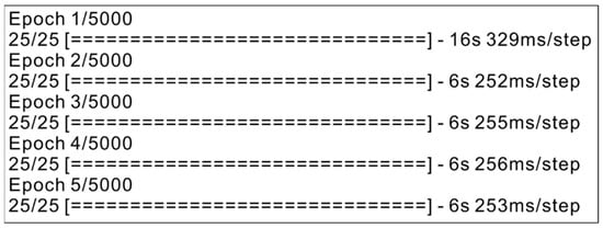
Figure 34.
Training time of the first five epochs using CPU.
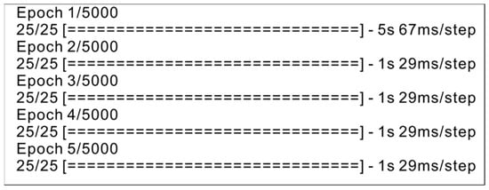
Figure 35.
Training time of the first five epochs using GPU.
From Figure 34 and Figure 35, it is evident that the GPU significantly outperforms the CPU in terms of training time. This discrepancy can be attributed to the GPU’s superior computing power and memory bandwidth, enabling more efficient parallel computing and faster model training. As a result, GPUs are well-suited for training deep learning models.
Based on the training results presented in Section 4.1 and Section 4.2, the LSTM and LSTM-NN training model is selected for prediction. The prediction data employs the last 5% of the dataset as the prediction set. Figure 36 and Figure 37 display the prediction results, while Figure 38 and Figure 39 illustrate the training time for the first five epochs, respectively. With the observed discrepancy in prediction accuracy for +1 and −1, our dataset has been meticulously crafted to maintain a balanced representation of convergence outcomes, ensuring that both +1 and −1 solutions are adequately represented. However, due to the inherent nature of the Duffing equation, the behavior of this equation can be highly complex and dependent on the initial conditions. We have also considered the use of class weighting techniques to address the class imbalance issue. This approach allows the model to assign higher importance to the minority class (in this case, either +1 or −1) during training, which can help mitigate accuracy discrepancies. We acknowledge that alternative evaluation metrics that consider class imbalance, such as F1-score, precision–recall curves, or area under the receiver operating characteristic curves (AUC-ROC), could provide a more comprehensive assessment of our model’s performance. The prediction results indicate that when the LSTM model predicts a value of −1, the accuracy rate reaches 96% compared to the true value. However, when both the predicted and actual values are 1, the accuracy drops to 86%. On the other hand, the LSTM-NN model achieves an accuracy rate of 87% for a predicted value of −1, while reaching 98% when both the predicted and actual values are 1. Figure 36 and Figure 37 demonstrate that the model with a hidden layer of neurons in the prediction process attains higher accuracy. Throughout the training process, the LSTM-NN model exhibits better and more stable performance compared to the LSTM model.
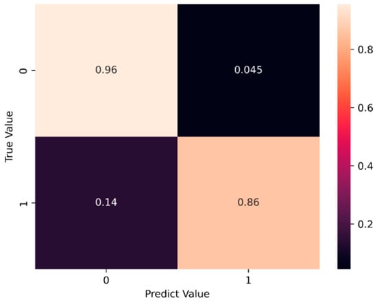
Figure 36.
LSTM model prediction results.
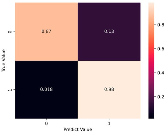
Figure 37.
LSTM-NN model prediction results.
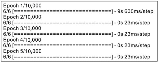
Figure 38.
The training time of the first five epochs of the LSTM model.
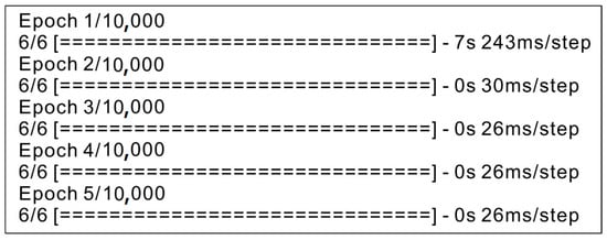
Figure 39.
The training time of the first five epochs of the LSTM-NN model.
Table 6 shows the confusion matrices values for the undamped system. The LSTM-NN model outperforms the LSTM model in predicting both +1 and −1 cases with higher accuracy. For predicting +1, LSTM-NN achieves an accuracy of 98%, whereas LSTM achieves 86%. In predicting −1, LSTM-NN maintains an accuracy of 87%, while LSTM has 96%. The loss values provide further insights into model performance. For predicting +1, LSTM-NN exhibits lower loss (1.8%) compared to LSTM (14%). In predicting −1, LSTM-NN still has lower loss (13%) compared to LSTM (4.5%). These results indicate that the LSTM-NN model not only achieves higher accuracy but also lower loss in both +1 and −1 prediction scenarios for the undamped system. This suggests that the LSTM-NN model is more effective in predicting binary outcomes in this context.
Table 6.
Confusion matrices values for the undamped system.
Figure 38 and Figure 39 illustrate that the LSTM-NN model has a longer training time than LSTM due to the inclusion of a larger number of hidden layers and neurons. While the LSTM model offers the advantage of faster training speed, its performance in handling binary classification datasets can be enhanced by incorporating hidden layers of neurons, leading to the LSTM-NN model. This modification improves the training and prediction outcomes significantly.
5.2. Duffing Equation Damped and Forced Vibration Type
After training the models in Section 4.3 and Section 4.4, we proceed to predict the single-cycle convergence results in the Duffing equation dataset containing damping and external force, using the prediction set. Both the LSTM model and the LSTM-NN model are utilized for this prediction. Figure 40, Figure 41, Figure 42 and Figure 43 display the results of predicting the maximum velocity, minimum velocity, maximum displacement, and minimum displacement using the LSTM and LSTM-NN models, respectively.
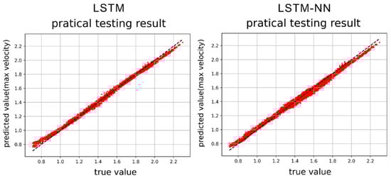
Figure 40.
Max. velocity prediction results by LSTM and LSTM-NN models.
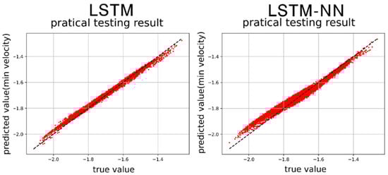
Figure 41.
Min. velocity prediction results by LSTM and LSTM-NN models.
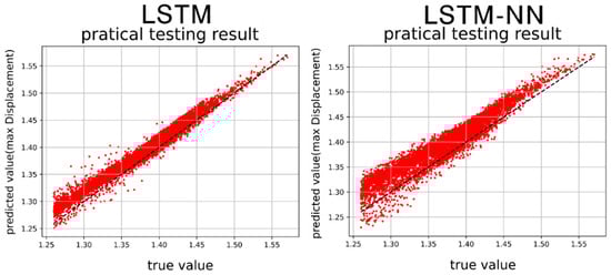
Figure 42.
Max. displacement prediction results by LSTM and LSTM-NN models.
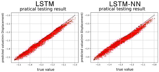
Figure 43.
Min. displacement prediction results by LSTM and LSTM-NN models.
Figure 40, Figure 41, Figure 42 and Figure 43 present the prediction graphs, with the horizontal axis representing the actual value and the vertical axis representing the predicted value. The dashed line represents the baseline where the actual value is equal to the predicted value. These figures provide an overview of the prediction results for the two models. Upon analyzing the training phase, it becomes evident that the LSTM-NN model performs better during training. However, the prediction results are not as satisfactory, indicating an overfitting problem during training for the LSTM-NN model. Notably, the prediction accuracy for velocity is noticeably higher compared to displacement. This discrepancy may arise due to the model’s insensitivity in capturing the data characteristics of displacement or the presence of poor-quality displacement data, resulting in inferior prediction performance. Between the two models, the LSTM model demonstrates superior accuracy compared to the LSTM-NN model.
Table 7 shows the error analysis for the damped System by MSE (mean-square error) and RMSE (Root mean square error). For the case of maximum displacement (Max Displ.): LSTM model achieves a MSE of 0.0484, while LSTM-NN has a higher MSE of 0.0953. The LSTM model has a RMSE of 2.1993, whereas LSTM-NN’s RMSE is higher at 3.0871. For the case of maximum velocity (Max Vel.): the LSTM model exhibits a MSE of 0.0527, whereas LSTM-NN has a higher MSE of 0.0960. The LSTM model records a RMSE of 2.1812, while LSTM-NN has a higher RMSE of 3.0988. For the case of minimum displacement (Min Displ.): the LSTM model achieves a MSE of 0.0476, while LSTM-NN has a higher MSE of 0.0958. The LSTM model has a RMSE of 2.2967, whereas LSTM-NN’s RMSE is higher at 3.0948. For the case of minimum velocity (Min Vel.): the LSTM model exhibits a MSE of 0.0381, whereas LSTM-NN has a higher MSE of 0.0789. The LSTM model records a RMSE of 1.9507, while LSTM-NN has a higher RMSE of 2.8091. The average of all parameters shows that: the LSTM model achieves an average MSE of 0.0467, whereas LSTM-NN has a higher average MSE of 0.0915. The LSTM model records an average RMSE of 2.1570, while LSTM-NN has a higher average RMSE of 3.0225. These results indicate that, in the damped system, the LSTM model generally outperforms LSTM-NN in terms of MSE and RMSE across all parameters. This suggests that the LSTM model provides more accurate predictions for the damped system compared to LSTM-NN.
Table 7.
MSE and RMSE error analysis fir the damped system.
Furthermore, the training time for both models can be observed in Figure 44 and Figure 45. Based on the comparison of prediction accuracy and training time presented in Figure 44 and Figure 45, it becomes evident that the LSTM model offers the advantages of shorter training time and high prediction accuracy. However, one drawback of LSTM models is that they may exhibit large fluctuations in training accuracy. On the other hand, the LSTM-NN model showcases stable training accuracy without significant ups and downs. However, when it comes to prediction accuracy, the LSTM-NN model falls short compared to the general LSTM model, particularly when dealing with multiple solutions. In summary, while the LSTM model excels in terms of training time and prediction accuracy, it is prone to fluctuations in training accuracy. Conversely, the LSTM-NN model maintains stable training accuracy but exhibits less accurate predictions, particularly for multiple solutions. Our study primarily focuses on predicting convergence outcomes of the Duffing equation, encompassing cases of +1, −1, and limit cycle oscillations (LCOs). These scenarios are commonly encountered in engineering problems involving nonlinear oscillations. However, it is important to note that our study does not cover cases of chaos or divergence, as they fall outside the scope of this research. The applicability of our models is best suited for scenarios where engineers or researchers need to predict the convergence behavior of systems described by the Duffing equation, which includes situations like aircraft wing vibrations or mechanical component oscillations. Regarding assumptions, we assume that the Duffing equation accurately represents the underlying dynamics of the systems being modeled. Additionally, we assume that the data used for training and validation is representative of real-world scenarios. While our models have shown promising results within the scope of our study, it is important to exercise caution when applying them to systems significantly deviating from the assumptions we have outlined above.
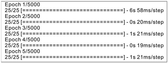
Figure 44.
The training time of the first five Epochs of the LSTM model.
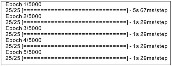
Figure 45.
The training time of the first five Epochs of the LSTM-NN model.
On considering computational cost, it is important to highlight that our chosen model, the Long Short-Term Memory (LSTM) model, demonstrates notable computational efficiency and low complexity. Firstly, during the training process, we observed that the LSTM model achieved high accuracy within a relatively short amount of time. In fact, as previously mentioned, using a GPU for training proved to be significantly faster compared to a CPU, showcasing the model’s computational efficiency. Please see Figure 34 and Figure 35. Secondly, the LSTM architecture is known for its capability to handle sequential data with relatively low computational overhead. This efficiency is due to the architecture’s inherent ability to capture and retain important information over time, making it suitable for problems like predicting the convergence outcomes of the Duffing equation. Additionally, our model’s straightforward architecture, involving a few hidden layers, contributes to its computational simplicity. This simplicity not only aids in efficient training, but also ensures that the model’s inference time, i.e., the time required to make predictions once the model is trained, remains reasonably low. Considering these factors, we can confidently assert that our LSTM model strikes a balance between predictive accuracy and computational efficiency. It offers high accuracy in predicting complex convergence patterns while maintaining efficient training and inference times. Therefore, it effectively addresses the trade-offs involved in model selection, aligning with the study’s objectives and requirements.
6. Conclusions
This study investigates the convergence results of the Duffing equation in two scenarios: undamped free vibration and damped forced vibration. The RK-4 method is utilized to collect data and mark the convergence results for undamped free vibration. Subsequently, the Long Short-Term Memory (LSTM) and LSTM-Neural Network (LSTM-NN) methods are employed for training and prediction to identify the best results. Moving on, the study examines the convergence results of the Duffing equation for damped forced vibration, considering various convergence characteristics, particularly focusing on the range of single-cycle convergence results. The collected data are compiled into a dataset, and the LSTM and LSTM-NN models are established to train and predict multiple solutions for the Duffing equation with damped forced vibration. From this study, several conclusions are drawn:
- When training the LSTM model, careful consideration must be given to the number of hidden layers, neurons, and epochs. While increasing these parameters may lead to improvements on the training set, there is a risk of overfitting on the validation set. Therefore, selecting the optimal number of layers, neurons, and epochs is essential to ensure efficient training and optimal performance on both the training and validation sets.
- To address the issue of over-reliance on training data and mitigate overfitting, incorporating a dropout layer into the basic model structure is recommended. The dropout layer enhances training stability by preventing excessive dependence on specific neurons, reducing the risk of overfitting.
- When selecting computing hardware for LSTM model training, using a GPU can significantly reduce the training time. GPUs are equipped with more cores and higher memory bandwidth, facilitating parallel execution of multiple matrix operations. This characteristic makes GPUs highly suitable for training deep learning models, efficiently handling the extensive computations involved in these models. Consequently, opting for GPU acceleration can lead to substantial time savings during LSTM model training.
- In this study, LSTM models were employed to train a specific dataset of undamped and unforced Duffing equation convergence results. The achieved accuracy was 95%, although it exhibited some fluctuations. To address this, neural network hidden layers were incorporated into the LSTM model, creating the LSTM-NN model. This modification improved the accuracy to 96% and mitigated the issue of accuracy fluctuations. However, it is worth noting that the increased number of hidden layers resulted in longer training times.
- In this study, the LSTM model was utilized to train a dataset containing convergence results of the Duffing equation with damping and external forces, focusing on single-cycle solutions. The accuracy achieved was 97.5% with fast training speed. By incorporating hidden layers of neurons (LSTM-NN), the training accuracy increased to 98% with lower loss. However, it is important to acknowledge that training time was prolonged due to the inclusion of a larger number of hidden layers.
- The LSTM model established in this study can predict the special case of the convergence result of the Duffing equation without damping and no external force. When the predicted value is +1, the accuracy reaches 96%, and when the value is −1, the accuracy also reaches 86%. The model with a hidden layer of neurons was 87% accurate on +1 predictions and 98% accurate on −1 predictions. The LSTM model after adding the hidden layer of neurons (LSTM-NN) is more suitable for predicting binary data sets.
- The LSTM model established in this study has a large deviation in the predicted displacement range when predicting the convergence range of the single-cycle Duffing equation containing damping and external forces, but has better performance in predicting the range of velocity (the case of multi-solution prediction). The model after adding the neuron hidden layer (LSTM-NN) also has the same situation, but the prediction accuracy is lower than that of the general LSTM model.
Author Contributions
Conceptualization, methodology, validation, formal analysis, investigation, writing—original draft preparation, Y.-R.W.; analysis, investigation, visualization, G.-W.C. All authors have read and agreed to the published version of the manuscript.
Funding
This research was supported by the National Science and Technology Council of Taiwan, Republic of China (grant number: NSTC 112-2221-E-032-042).
Institutional Review Board Statement
Not applicable.
Informed Consent Statement
Not applicable.
Data Availability Statement
Not available.
Conflicts of Interest
The authors declare no conflict of interest.
References
- Feng, G.Q. He’s frequency formula to fractal undamped Duffing equation. J. Low Freq. Noise Vib. Act. Control 2021, 40, 1671–1676. [Google Scholar] [CrossRef]
- Rao, S.S. Chapter 13 Nonlinear vibration. In Mechanical Vibrations, 6th ed.; Pearson Education, Inc.: New York, NY, USA, 2017; pp. 1134–1169. [Google Scholar]
- Akhmet, M.U.; Fen, M.O. Chaotic period-doubling and OGY control for the forced Duffing equation. Commun. Nonlinear Sci. Numer. Simul. 2012, 17, 1929–1946. [Google Scholar] [CrossRef]
- Hao, K. We Analyzed 16,625 Papers to Figure Out Where AI Is Headed Next. MIT Technology Review, 25 January 2019. Available online: https://www.technologyreview.com/2019/01/25/1436/we-analyzed-16625-papers-to-figure-out-where-ai-is-headed-next/ (accessed on 13 September 2023).
- Hinton, G.E.; Osindero, S.; Teh, Y.-W. A fast learning algorithm for deep belief nets. Neural Comput. 2006, 18, 1527–1554. [Google Scholar] [CrossRef] [PubMed]
- Hinton, G.E. Learning multiple layers of representation. Trends Cogn. Sci. Rev. 2007, 11, 428–434. [Google Scholar] [CrossRef] [PubMed]
- Hinton, G.E.; Srivastava, N.; Krizhevsky, A.; Sutskever, I.; Salakhutdinov, R.R. Improving neural networks by preventing co-adaptation of feature detectors. arXiv 2012, arXiv:1207.0580. [Google Scholar] [CrossRef]
- Kingma, D.P.; Ba, J. Adam: A method for stochastic optimization. arXiv 2015, arXiv:1412.6980. [Google Scholar] [CrossRef]
- Srivastava, N.; Hinton, G.E.; Krizhevsky, A.; Sutskever, I.; Salakhutdinov, R. Dropout: A simple way to prevent neural networks from overfitting. J. Mach. Learn. Res. 2014, 15, 1929–1958. [Google Scholar]
- Potdar, K.; Taher, S.P.; Chinmay, D.P. A comparative study of categorical variable encoding techniques for neural network classifiers. Int. J. Comput. Appl. 2017, 175, 7–9. [Google Scholar] [CrossRef]
- Mathia, K.; Saeks, R. Solving nonlinear equations using Recurrent Neural Networks. In Proceedings of the World Congress on Neural Networks (WCNN’95), Washington, DC, USA, 17–21 July 1995; Renaissance Hotel. pp. 76–80. [Google Scholar]
- Hochreiter, S.; Schmidhuber, J. Long short-term memory. Neural Comput. 1997, 9, 1735–1780. [Google Scholar] [CrossRef] [PubMed]
- Han, J.; Arnulf, J.; Weinan, E. Solving high-dimensional partial differential equations using deep learning. Proc. Natl. Acad. Sci. USA 2018, 115, 8505–8510. [Google Scholar] [CrossRef] [PubMed]
- Wang, Y.R.; Wang, Y.J. Flutter speed prediction by using deep learning. Adv. Mech. Eng. 2021, 13, 16878140211062275. [Google Scholar] [CrossRef]
- Gawlikowski, J.; Tassi, C.R.; Ali, M.; Lee, J.; Humt, M.; Feng, J.; Kruspe, A.; Triebel, R.; Jung, P.; Roscher, R.; et al. A survey of uncertainty in deep neural networks. arXiv 2022, arXiv:2107.03342. [Google Scholar] [CrossRef]
- Hua, Y.; Zhao, Z.; Li, R.; Chen, X.; Liu, Z.; Zhang, H. Deep learning with long short-term memory for time series prediction. arXiv 2018, arXiv:1810.10161 [cs.NE]. [Google Scholar] [CrossRef]
- Hwang, K.; Sung, W. Single stream parallelization of generalized LSTM-like RNNs on a GPU. arXiv 2015, arXiv:1503.02852. [Google Scholar] [CrossRef]
- Zheng, B.; Vijaykumar, N.; Pekhimenko, G. Echo: Compiler-based GPU memory footprint reduction for LSTM RNN training. In Proceedings of the 47th Annual International Symposium on Computer Architecture (ISCA), Virtual Event, 30 May–3 June 2020; IEEE: Piscataway, NJ, USA, 2020; pp. 1089–1102. [Google Scholar] [CrossRef]
- Tariq, S.; Lee, S.; Shin, Y.; Lee, M.S.; Jung, O.; Chung, D.; Woo, S.S. Detecting anomalies in space using multivariate convolutional LSTM with mixtures of probabilistic PCA. In Proceedings of the 25th ACM SIGKDD International Conference on Knowledge Discovery & Data Mining, Anchorage, AK, USA, 4–8 August 2019; pp. 2123–2133. [Google Scholar]
- Memarzadeh, G.; Keynia, F. Short-term electricity load and price forecasting by a new optimal LSTM-NN based prediction algorithm. Electr. Power Syst. Res. 2021, 192, 106995. [Google Scholar] [CrossRef]
- He, C.-H.; El-Dib, Y.O. A heuristic review on the homotopy perturbation method for non-conservative oscillators. J. Low Freq. Noise Vib. Act. Control 2022, 41, 572–603. [Google Scholar] [CrossRef]
- Wang, K.-J.; Si, J. Dynamic properties of the attachment oscillator arising in the nanophysics. Open Phys. 2023, 21, 20220214. [Google Scholar] [CrossRef]
- Wang, K.-J.; Wang, G.-D. Gamma function method for the nonlinear cubic-quintic Duffing oscillators. J. Low Freq. Noise Vib. Act. Control 2022, 41, 216–222. [Google Scholar] [CrossRef]
- Zayed, S.M.; Attiya, G.; El-Sayed, A.; Sayed, A.; Hemdan, E.E. An efficient fault diagnosis framework for digital twins using optimized machine learning models in smart industrial control systems. Int. J. Comput. Intell. Syst. 2023, 16, 69. [Google Scholar] [CrossRef]
- Zhang, Y.; Ji, J.C.; Ren, Z.; Ni, Q.; Gu, D.; Feng, K.; Yu, K.; Ge, J.; Lei, Z.; Liu, Z. Digital twin-driven partial domain adaptation network for intelligent fault diagnosis of rolling bearing. Reliab. Eng. Syst. Saf. 2023, 234, 109186. [Google Scholar] [CrossRef]
Disclaimer/Publisher’s Note: The statements, opinions and data contained in all publications are solely those of the individual author(s) and contributor(s) and not of MDPI and/or the editor(s). MDPI and/or the editor(s) disclaim responsibility for any injury to people or property resulting from any ideas, methods, instructions or products referred to in the content. |
© 2023 by the authors. Licensee MDPI, Basel, Switzerland. This article is an open access article distributed under the terms and conditions of the Creative Commons Attribution (CC BY) license (https://creativecommons.org/licenses/by/4.0/).