Abstract
This paper proposes a method to reduce seismogram variability as a determining factor in its interpretation, processing, and clustering. By introducing the concept of single fluctuations (SFs), the seismogram can be parsed into a sequence of random impulses with subsequent ordering. This rearrangement of SFs, if they are assigned by positive integers, represents the formal mapping of a regular string of integers into a random one, which can be represented with a bipartite random graph (bigraph). Due to its specific randomness, such a bigraph is considered a new type of random balanced bigraph. The R-envelope and RQ-envelope, its equidistant version, are defined by tracing the peak envelope over ordered SFs. The equivalence and complementariness of the RQ and bigraph are considered and discussed, forming a combined characteristic of the seismogram. The R/RQ provided a considerable reduction in seismogram variability, which was confirmed by creating and analyzing an ensemble of RQ from several seismograms. In the RQ domain, distance is defined as a possible basis for metrics and clustering, but the ensemble variability was quite narrow and not as suitable for this purpose. Otherwise, the ensemble shows high redundancy hidden in the seismogram population. As for the bigraph, the mesh of its edges is structuralized in bundles, forming a skeleton, which reflects the internal structural content of the seismogram. The distance over the domain of bigraphs is proposed to show the possibility of clustering. This means that only a combined RQ and bigraph provides a suitable frame for seismogram representation with reduced variability and, thus, the potential for more effectively organizing seismic databases and a deeper interpretation of seismograms; therefore, RQs and bigraphs can be considered as a transform of a seismogram. Many aspects of these concepts are thoroughly discussed. The similarity between concepts of SF and wavelets is briefly considered. This very complex theme is new and promises broad further research. All issues considered in the paper are abundantly illustrated.
1. Introduction
Earthquakes can inflict heavy damage and human casualties. Related disciplines have studied earthquakes to widen and deepen understanding of the phenomenon. There is a natural hierarchy in this complex study. At the top is seismology (geoscience), which studies earthquakes as intrinsic processes (see, e.g., [1,2,3]). The next layer, which relies on the findings and extensive knowledge of the previous discipline, deals with earthquake risk reduction and hazard assessment, creating a basis for the majority of activities in societies that can be affected by earthquakes. There is immense literature related to this area of knowledge, which indicates a high interest of humankind in these effects. This work presents and briefly discusses just a few examples, chosen in a semi-random manner, to help create a representation in this area. For example, the German GFZ (GeoForschungsZentrum, (eng) Research Centre for Geosciences) provides seismic hazard maps [4] as products of the Global Seismic Hazard Assessment Program started in 1993 [5]. The basis for these hazard maps is the seismic database. As for particular research in this area, the references [6,7,8,9,10,11] are typical and illustrative. There is also a large amount of general literature, including the authors’ favorite [12], which covers the transition from hazard to seismic-resistant civil engineering, aimed to alleviate the seismic vulnerability of the built environment [13,14,15].
The acquired knowledge gradually improves planning, designing, and constructing structures according to the developing standards of earthquake resilience [12]. The perpetual updating of regulations and standards for designing and building structures is derived from the study of earthquakes themselves and the effects they cause on existing structures.
A seismogram contains almost all one can really know about an earthquake, apart from the effects people see, feel, or suffer. It is a recorded waveform of seismic effects at a site, representing fluctuations of related physical (mechanical) quantities as the result of many complex processes taking place in the so-called “information chain” of seismology, with many interrelated sub-systems such as the seismic source, wave propagation through the Earth, distortion by other seismic signals, and the influence of seismic sensors, recorders, and processing techniques on the seismogram [1] “Ch. 1, Figure 1.2, p. 6”. An excellent survey of all the phenomena involved can be found in [1] “Ch. 11”. The influence of propagation conditions on a waveform’s appearance in different seismograms that all originate from the same event can be seen in [16] “Figures 5 and 6”.
Therefore, seismogram databases contain all the accumulated intrinsic knowledge of seismicity, where earthquakes are classified according to various criteria, i.e., parameters. Databases are the main sources of seismic information for experts from various branches of knowledge interested in earthquakes and their effects, who then transform these raw data into respective findings, rules, recommendations, and assessments, often incorporated into regulations. These experts include geophysicists, seismologists and observatory personnel, civil engineers, disaster managers, risk planners, urban planners, and governments, not to mention related researchers, students, and training personnel [1] “Ch. 1, pp. 29”, [12,17].
Any earthquake in a database is represented by at least one or up to several seismograms and accompanying parameters. Seismic databases can be conditionally categorized as general and specific by content, and as global and local by cover. A typical example of general/global is the PEER Ground Motion Database [18]. The use of the PEER database motivated the authors to conduct this research. Accordingly, this database is the main reference and the main frame for seeking solutions. Also, as the authors have been able to see, other seismic databases are organized on the same principles with the same parametric nomenclature, i.e., on parametric attributes of seismograms (one number for the whole complex waveform). Examples span from specific/local databases [19,20] to general ones [21]. Global databases often redirect the user to local (national) databases [21]. Seismograms are usually given in the form of time series and the spectrum. The spectrum can be considered an ordered picture of the seismogram; nevertheless, both are of random appearance. Considering their shapes, it is apparent that the variability of seismograms is more prominent than that of their spectral counterparts. Therefore, the spectrum is more suitable for practical use, so it appears as the main characteristic of earthquakes in databases.
Difficulties of classification within certain populations rise with the variability of population elements. This is particularly true for seismograms and the system in which they are grouped in databases.
During earlier research on seismograms related to defining seismogram’s new attributes, the authors made some interesting findings, which can improve grouping (clustering) criteria. The idea is based on treating the seismogram as composed of random impulses. Recomposing random impulses trained into an ordered sequence can be described as random mapping and represented through a random bipartite graph of a specific kind. Such structuralization of a seismogram significantly reduces its inherent variability and yields certain new characteristics that can be used to improve it by adding to existing grouping criteria (classification) in seismic databases.
1.1. Brief about Bipartite Graphs
Random graphs are very useful and universally applicable mathematical tools. Their offspring, termed complex networks, with more structurality and dynamics, are even more capable of describing the world, which can be considered as being composed of ‘systems of systems’ and is tremendously versatile and intricate. Among the vast literature, we quote several typical references [22,23,24,25,26,27,28,29,30].
There are many types of random graphs/networks, such as bipartite random graphs, that have been recognized as particularly insightful representations of many different systems [31,32].
The case presented in this paper, as far as we know, describes a specific application of bipartite graphs not found in the literature until the present day. It involves randomness in such an unusual way, in comparison to existing models, that we were inclined to consider it a new type of random bipartite graph. It falls somewhere between conventional and random bigraphs.
In a bipartite graph (bigraph for short), vertices (nodes) can be divided into two disjoint sets such that no edge connects two vertices of the same set [31].
Generally, two categories of bipartite graphs can be distinguished: conventional and random. In the first, graphs show all existing edges between input and output vertices, while random graphs show possible or potential edges between vertices. Basically, two classical models for random graphs are used: G(N, L), where N vertices are connected with L randomly placed links [24], and G(N, p), where each pair of N vertices is connected with probability p [25].
The core of these models is the fact that random graphs (networks) are statistical ensembles of graphs, where each one has its specific probability of realization [28].
A balanced bipartite graph is one that has an equal number of vertices in both sets, which will be of particular interest in our investigation [31]. Further details can be found in various references [28].
Different terms for basic structural elements of graphs, ‘node’, ‘vertex’, ‘link’, or ‘edge’, will be used throughout the text.
Regarding nodes, we have to name the two separate sets of nodes of the bipartite graph according to their disposition. The usual graphical representation of these node sets is a linear array of small circles (bold points), where linearity stems from a mapping domain (interval) on an axis and also provides the most transparent outlook of the ‘mesh’ of edges between input and output nodes. The issue of node disposition contains some interesting aspects.
Linearly disposed nodes are usually arranged in a left–right configuration as two vertical columns. More deeply, it hides the causality orientation of the mapping process: the start of mapping is in the left column, and the end of mapping is in the right one. There is also the vertical disposition, where the beginning set is up, and the end set is down. This defines the implicit direction of the graph.
We will use the terms ‘input’ and ‘output’ for sets of vertices (nodes) and adopt vertical disposition as more adequate for our case since the seismogram, taken as a sequence of random impulses, is always presented horizontally.
Despite their seemingly plain geometry, bipartite graphs include many families of different structures [32]. There are many other ways of describing random bipartite graphs using simpler characteristics.
One usually tends to describe any complex entity through simpler properties in order to analyze it in an easier way. Generally, many properties of random graphs are defined and measured, such as diameter, the longest shortest path, average path length, degree distribution, clustering coefficient, etc. More complete and descriptive characteristics are, e.g., the adjacency matrix and the graph spectrum [33,34]. Even the form in which a graph is depicted can be considered a graph property, which is very helpful in its description. The very name ‘graph’ carries pictorial or geometrical meaning. Also, the adjacency matrix is not just a numerical presentation of the graph but brings a pictorial aspect to the graph’s structure.
The random graph proposed in this paper is designated as a seismogram transform, which represents an ordered and simplified seismogram description with greatly reduced original variability, which we expect to be more suitable for organizing seismic databases, which are the fundamental information sources for experts from various knowledge areas.
1.2. Article Goals and Basic Findings
The immense variability of seismograms prevents the effective organization of seismic databases to ease the retrieval of systematic knowledge about seismicity in general, known as data mining or metadata extraction [35].
The issue of proper organization of a seismic database is a very complex matter, but that does not mean that one should not cope with it.
The main idea supporting this research is not to use only the simple parametric attributes of seismograms for grouping (clustering) but to go deeper into the seismogram’s structure and propose more complex characteristics suitable for effective clustering.
Identifying the variability as the main factor in solving the problem, the authors will try to find methods of reducing it, thereby hoping to facilitate grouping. Therefore, the term ‘potential’ in the article’s title, indicating conditional relation, means either more or less suitability of the approach.
A few ideas defining the steps of seismogram processing are proposed, which can be assembled into one approach, yielding new characteristics of the seismogram with far less variability than the intrinsic ones found in the seismogram itself. These are the bigraph and its equivalent, better to say its complement, named the R-envelope. Both are based on parsing the seismogram into single random impulses, i.e., elementary/single fluctuations (EF/SF), and the subsequent ordering of SFs to give the said characteristics. The coherence between these two compelled the authors to qualify this approach as the transform.
The presented results confirm the reduced variability. It is more prominent in RQ. The variability range is narrow, reminiscent of an invariant. This finding deserves thorough further research.
As for the bigraph, the range of variability possesses not only one degree of freedom, as in the case of RQ but a few more, residing in the system of bundles of edges, recognized in the mesh of edges in the bigraph. The structural information of the seismogram is, thus, preserved in the bigraph. Thus, the meaning of the article’s title denotes the new type of bigraph as a transform of seismograms. On the other hand, it does not lessen the importance of RQ, which found its place in the Graphical Abstract of this paper in the designation RQ⊕BG.
Because of its new characteristic(s), it was necessary to consider it from various aspects to better describe its properties and applicability.
2. Materials and Methods
2.1. Seismogram as a Sequence of Random Impulses
As stated in the Introduction, a seismogram is the result of many complex processes taking place in the so-called “information chain” of seismology, from the earthquake source to the recording place.
Considered only by its appearance, the waveform, a seismogram is a fluctuational transient of certain mechanical quantities (acceleration, velocity, displacement), where the waveform looks as if it is composed of random impulses [2] “Vol. 1, paper 1.03.1.3, pp. 73, 131”, with random amplitudes, durations, and shapes. Although the term “fluctuation” (to fluctuate) refers to the irregular rising and falling (change) of a physical quantity, we will further formalize this term and introduce the concept of elementary fluctuation (EF), consisting of “ups” and “downs”, separated by crossings of a certain axis (usually the t-axis). Hence, the seismogram is considered a sequence of EFs since an alternating pattern, although random, occurs in its waveform.
In this sense, the EF is usually composed of two subsequent alternate random impulses, which we will call single fluctuations (SFs).
To put it more clearly:
Therefore, the EF, or the SF, is the basic structural element of the seismogram (see Figure 1).
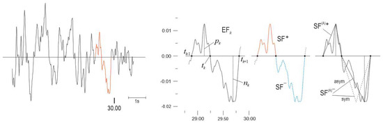
Figure 1.
(left) A fragment from the seismogram of the RSN 1616 event, Düzce, Turkey, shows the complex random behavior of the seismic process. Units on axes scales are in g and in s. The trace in red color indicates the concept of elementary fluctuation (EF) introduced in this paper. (right) The EF can be parsed into two single fluctuations (SFs) as a pair of positive (red line) and negative (blue line) random impulses. (far right) Geometrical approximation of SFs by symmetric (sym) and asymmetric (asym) triangles.
For numerical simplification, we express the complex waveform of SFs with two parameters: the maximum amplitude of the SF and its duration (Figure 1), which, geometrically, is equivalent to the approximation of SFs by respective triangles, either symmetrical or asymmetrical (Figure 1). In other words, a seismogram is represented by a non-equidistant sequence of amplitude samples and is a sort of non-uniform sampling.
When we speak of geometry, we will distinguish intrinsic SFs and approximated (by triangles) SFs, which are labeled as SF and SF(A), respectively.
The concept of the EF or SF enables the parsing of a given seismogram into a sequence of SFs, which is a very important operation. Notice that, from the point of view of this research, it is the same as if the whole seismogram waveform is parsed directly into SFs or, after an interstep of approximation, into respective triangles.
After segmentation, the seismogram is actually divided (separated) into two sequences of SFs (or respective triangles SF(A)s), one comprising only SFs with positive amplitudes and another with negative amplitudes. This can be described in terms of the set theory and is a nice example of set theory application.
The original set of SFs is divided into two disjoint subsets:
As a next step of the procedure, elements of each of these sequences are assigned with integers:
where I is the index set (Figure 2) (see, e.g., [36]).
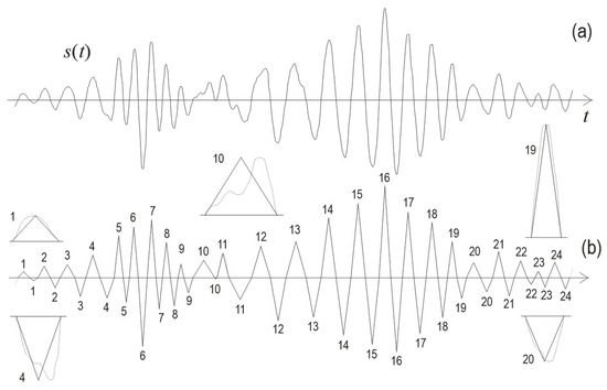
Figure 2.
(a) Seismogram waveform s(t) is composed of random impulses. (b) Approximation by (symmetric) triangles is geometrically equivalent to the numerical reduction of each random impulse to its maximum amplitude and duration. Further reduction involves assigning positive integers to positive and negative triangles. Zoomed-in examples of approximated and indexed SFs (positive: 1, 10, 19, and negative: 4, 20) are inserted around approximated waveform. The original SFs are depicted by dash line.
Similarly, these relations can be easily rewritten for triangles approximating the SFs.
2.2. Ordering of SFs
Having indexed sets of SFs, or SF(A)s, both positive and negative, the next operation is applied: the ordering of each SF(A) sequence by maximum amplitude. For clarity, the ordering is only applied to positive SFs, which is presented in Figure 3.
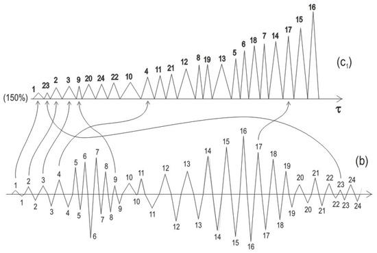
Figure 3.
Rearrangement (ordering) of positive SF(A)s, from approximated waveform (b), retaken from Figure 2, by maximum amplitude, yields the waveform (c1). This means the ordered sequence of integers is mapped into a random sequence of integers, or a random sequence of triangles is mapped into an ordered sequence of triangles. The scale on the τ-axis of (c1) is zoomed in by 150% with respect to diagram (b).
A random sequence of SFs is converted into an ordered sequence of SFs, while the initial sequence of naturally ordered integers is turned into randomized indexes. This is obviously a kind of random mapping, which can be written as:
A similar relation can be written for triangles {SF(A)}
It is important to note that the approximation goes from the complex waveform of an SF down to an integer only, which is the ultimate level of approximation (simplification).
Thus, the ordering maps one sequence of integers into another one. This function is another form of mapping. It seems to be a dead end. Reducing either SFs or SF(A)s to integers, one gets simple, bare numbers and loses information for their mapping contained in their max amplitudes. How, then, to obtain an ordered set?
The answer is obvious, but it should be explicated: the amplitude information is hidden in the function that performs the mapping.
There, one finds the meaning of twofold digitizing of the seismogram: behind the sequence of integers is hidden a corresponding sequence of real numbers (SFs maximum amplitudes), which serve for the ordering operation.
Moreover, the mapping can be considered a sequential operation consisting of a pair of instantaneous acts: taking an input integer, applying the function, and obtaining the result—the output integer. Therefore, it is possible to represent the mapping, which includes input and output and the beginning and ending stages of the mapping process. This is the basis for representing such mapping with the bipartite graph, which shows all acting stages of function.
If reduced to the level of pure integers, the mapping (function) can be written as:
for positive SFs (or SF(A)s).
This kind of mapping can be represented with bipartite graphs (shown in Figure 4).
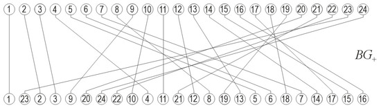
Figure 4.
A bipartite graph (vertical configuration), by its edges, connects input and output nodes assigned by integers so that the input ordered sequence shuffles into a random one. The bigraph structure schematically follows the mapping indicated on Figure 3. Such random mapping relies on SFs in the original seismogram and on their random maximum amplitudes.
2.3. New Type of Bipartite Graph as a Transform of Seismogram
2.3.1. Twin Bipartite Graph—Twofold Result of Transform
The previous section considered representation for only positive SFs (or SF(A)s) by corresponding bipartite graph (Figure 3 and Figure 4), mainly for the sake of procedure illustration. This means that a bipartite graph is created only for half of the seismogram. The same should be performed for negative SFs. Ordering and mapping (Figure 5) produce an additional bigraph, which means that the (whole) seismogram is represented by a pair of bipartite graphs (Figure 6).
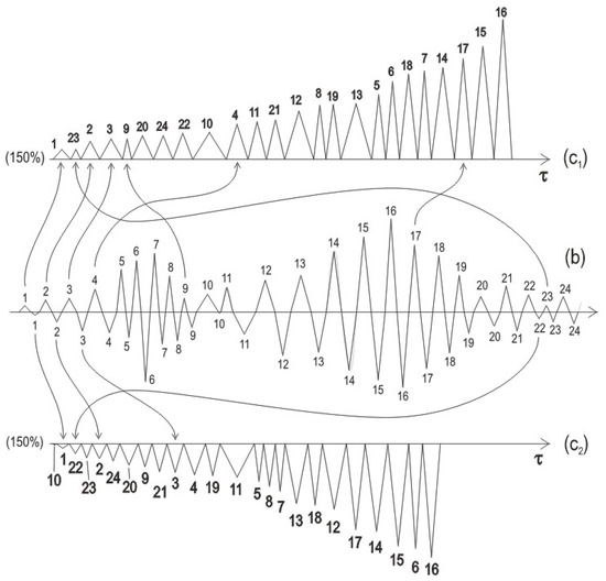
Figure 5.
Complete rearrangement of (approximated) seismogram from Figure 2 involves both positive and negative SF(A)s, whose mappings are clearly indicated by arrows. Notice that the positive and negative SF(A)s are indexed in the same manner, while the respective mappings produce different random sequences of integers. Summed durations of positive and negative SF(A)s are different.
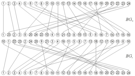
Figure 6.
The twin bigraph, composed of two bipartite graphs with two-row geometry, represents mappings (orderings) between sets of indices (integers) for positive and negative SFs, according to mappings on Figure 5. Both bigraphs are positioned in mirror vertical symmetry, where the bigraph BG− is inverted (input nodes down, output nodes up) to follow the general disposition of SFs in a seismogram.
Indexing SFs reduces their usually complex waveforms to integers, which means that the entire seismogram’s intricate waveform is described by two sequences of integers. In such a reduction of random impulse shapes, only the maximum amplitudes of SFs remain important as a factor for ordering purposes.
The seismogram can be considered as digitized in a twofold manner:
- As a sequence of integers;
- As a sequence of real numbers (maximum amplitudes of SFs, or of approximating triangles SF(A)s), whose positions within the sequence are implicitly marked by integers, i.e., indexes.
Splitting the whole seismogram into positive and negative SFs resulted in two separate bigraphs, one unique result of this procedure.
To overcome this inconsistency, one simply can consider them as united and transpose them into ‘the twin bigraph’ (Figure 6). There may be the impression that this is only semantic because they remain separated. However, the two bigraphs are not as separated as it may seem from Figure 6. In the background, they are quite correlated since they are parts of a singular seismogram.
Therefore, one can treat the ‘double’ result of these operations as a whole, as a singular mathematical entity, even though it comprises two actually separated bigraphs. Those two, to some extent, mirror each other so that all operations applied to the seismogram can be treated as a kind of transform.
The operator labeled by
stands for this transformation. The unity of two bigraphs, i.e., the twin bigraph, is labeled by the symbol ⊕, lent from XOR operation (addition modulo 2). Using the symbol ⊕ for such a purpose does not mean it executes this operation between two bigraphs strictly, but symbolizes the unity of these two mathematical objects and points out the fact that the two bigraphs should be considered as one. In addition, the operation ⊕ brings with it some combinatorial unifying of SF+s and SF−s, defined by its truth table, particularly for meaning “one or the other but not both”, which additionally vindicates the handy use of strictly defined operation.
Thus, one can write also:
Since the BG− is represented in Figure 6 as geometrically inverted, Equation (9) ought to be modified as:
In a nutshell, the transform essentially involves two mappings of integers, both for the positive and negative SFs, which can be designated as functions (bijections) F+ and F−
2.3.2. Coupled Twin Bigraph—Unifying the Twofold
It seems that this transform, as the result of splitting all SFs into positive and negative, produces two separate bigraphs, seemingly separated. They are called twins since there is an invisible unifying factor standing behind them—the seismogram itself. By transferring SFs into integer sequences, the connectedness between the twins fades, becoming less apparent; therefore, it is necessary to conjugate the twins in a more explicit way to make the connections more obvious.
One possibility is to connect the corresponding output nodes of positive and negative bigraphs, thus reestablishing structural relationships that existed in the seismogram at the level of EFs, i.e., EF = SF+ + SF−. What is the meaning of this proposal?
Actually, in this way, one gets three bigraphs that are overlapped. The two outer bigraphs, formerly the twin bigraphs, are now connected by a new bigraph, where it is not easy to define which nodes are input and which are output. Because of that fact, it deserves a special designation, FC, and a special name, the connecting bigraph (Figure 7). The whole structure is called the coupled twin bigraph.
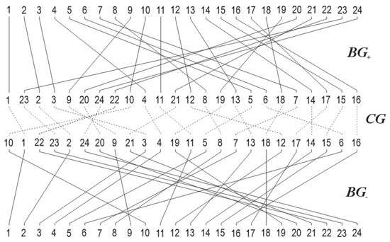
Figure 7.
The win bigraph from Figure 6 is unified into a singular entity over the connecting bigraph, which nodes are both output nodes of BG+ and BG−, making the coupled twin bigraph. Simultaneously, the connecting bigraph (CG) shows symmetry/asymmetry of the twin bigraph, i.e., of the whole seismogram.
This looks like a quadripartite graph: nodes are apparently partitioned into four sets. However, if one recalls the mirror structure of the twin bigraph, based on purposely dividing all SFs into positive and negative subsets where output sets stand opposite each other, there will hardly be any nodes left for a new bigraph, which is called a connecting bigraph.
Nevertheless, there is no paradox. Moreover, it can even be said that such uncertainty confirms the unity of the structure, and now not only in name, as in the case of the twin bigraph, but essentially, reflects the unity of the seismogram’s waveform at the integer level.
All previous is said following the bigraph geometry adopted in this paper, as a linear arrangement of nodes, vertically disposed, with input nodes positioned up and output nodes down, where the bigraphs in the twin bigraph are arranged with output nodes face to face. This configuration essentially follows the structure of a seismogram waveform composed of two sequences of SFs on both sides of the t-axis.
2.3.3. Bigraph of the Whole Seismogram
The coupled twin bigraph is proposed to overcome splitting the seismogram into two parts: positive and negative SFs.
There is another, more natural, way to represent the whole seismogram with a single bipartite graph. It is based on a simple operation applied to a certain waveform: rectification.
Mathematically, it is expressed by the modulus operation.
When negative amplitudes also become positive, then the ordering operation is made over the whole set of SFs, which can be seen in Figure 8. Now, the twin bigraph turns into a conventional balanced bipartite graph, which is presented in Figure 9, and, for distinction, is called an ‘absolute bipartite balanced graph’.
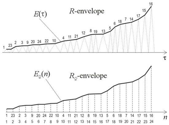
Figure 8.
(up) The envelope E(τ) is drawn over peaks of approximated positive SFs, i.e., over positive SF(A)s, and still contains information about time, designated as R-envelope. (down) The envelope EQ(n) is drawn over equidistant max amplitudes of SFs, making time information irrelevant, hence the label n at abscissa. It is called the RQ-envelope. Note two indexing strings along abscissa: positional (1, 23, 2, 3, 9, 20, …) and regular (1, 2, 3, 4, 5, …). Note also that the difference between correspondent integers of these two numerations (e.g., (20, 6), (24, 7), etc.) directly indicates the displacement length of max amplitude during the ordering process.
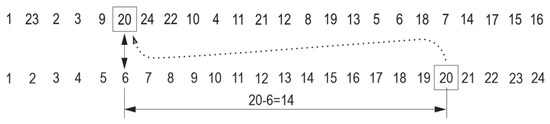
Figure 9.
Zoomed-in double indexing from Figure 8, positional and regular, clearly shows the magnitude of displacements of integers during the operation of ordering.
Using operator form, one can write:
2.3.4. Shuffle of the Twin Bigraf into Singular One
The rectifying operation applied to the seismogram waveform yields a unified (or absolute) bigraph. On the other hand, comparing meshes of edges in the twin bigraph and absolute bigraph, one can notice apparent similarities, which begs a natural question: Is it possible then to “rectify” and unify the twin bigraph to obtain a singular bigraph? How close are these two operations? In other words, can a modulus operation be applied to the twin bigraph itself?
Having on mind Equations (9) and (10), it seems that it is simply necessary to sum graphs A and B to obtain C. Before that, one needs to invert the bigraph BG− since it was turned in the twin graph. It can be written as:
The effect is shown in Figure 10.
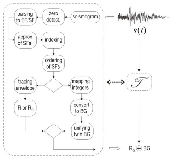
Figure 10.
Turning out the seismogram into the sequence of SFs is the basis for creating the RQ-envelope and the bigraph. All subsequent operations can be gathered into a transform of the seismogram, yielding a result composed of RQ and BG.
Obviously, if the size of the twin bigraph is N, then the size of the absolute graph is 2N, assuming an equal number of positive and negative SFs, i.e., the complete alternating structure of each EF = SF+ + SF−.
2.4. R-Envelope of Ordered Seismogram
In addition to the bigraph as an ordered representation of a seismogram, another characteristic can be introduced, which is also of pictorial appearance. Let its name be the R-envelope (R comes from ‘rearranged’). It is also a part of the general frame of this research. Its meaning is graphically explained in Figure 8.
Three forms of the R-envelope can be considered:
- Drawn over the peaks of SFs;
- Drawn over the peaks of SF(A)s (over peaks of approximating triangles);
- Drawn over equidistant maximum amplitudes.
In the first two cases, the factor of time also determines the shape of the R-envelope (different durations of SFs). In the third case, the time becomes irrelevant, so the abscissa can be designated as a simple numerical axis, as shown in Figure 8. Because of that, this form of R-envelope is designated as RQ-envelope (meaning ‘quantized’).
2.5. R/RQ-Envleope—Bigraph, Equivalence, or Complement?
While the graphical appearances of the bigraph and the R-envelope might seem different, they are deeply equivalent.
The bigraph obviously does not contain any information about time, as opposed to the R-envelope, either drawn over original SFs or over approximated SF(A)s: both contain data about durations of SFs. Therefore, the R-envelope is over-equivalent to bigraph and, hence, not truly equivalent.
On the other hand, in depicting the RQ-envelope, having all SF(A)s reduced to their maximum amplitudes (as samples) and equidistantly positioned along the abscissa, one can disregard the time and assign samples by integers, designating earlier positions of SFs in the rearranged seismogram.
Because of that, one simply puts a random sequence on integers along the abscissa.
As can be seen on Figure 9, each vertical pair of integers indicates the mapping (displacement) span, e.g., in the 6th column, one sees numbers 20 and 6, which means that the mapping span is 20 − 6 = 14, etc. By placing the regular indexing, or just identifying the linear address of a number along the abscissa (i.e., its position), one implicitly depicts the respective bigraph. In other words, the bigraph is contained (hidden) within these two strings of integers. This means that the diagram of the RQ-envelope contains its (equivalent) bigraph. This is a plain bigraph in which nodes and edges do not have weights.
This still does not mean that the RQ-envelope and respective diagram are fully equivalent since the RQ-envelope contains maximum amplitudes of SFs, or SF(A)s, the only residual from the seismogram in the RQ-envelope.
If one considers the weighted instead of the plain bigraph, where the weights of nodes represent maximum amplitudes of SFs, or SF(A)s, then a complete equivalence between the RQ-envelope and respective bigraph is attained.
In brief, the simple bigraph is a 2D structure, while the weighted bigraph is a 3D structure.
The claimed equivalence still seems suspicious since there are two very different mathematical objects to compare: one continuous (RQ-envelope), and another truly discrete (bigraph).
The point is that the RQ-envelope is seemingly continuous since it is not a monotonic curve but a polygonal line whose nodes are maximum amplitudes of SF(A)s. A polygonal line is composed of linear segments, and each segment is completely determined by its nodes, i.e., the coordinates of each point along a segment are determined by the coordinates of its ends (nodes). In other words, a polygonal line does not contain more information than the nodes that it is drawn through.
Therefore, the RQ-envelope is actually a string of numbers, the same as those assigned to the nodes of the bigraph, where the polygonal line is drawn only for better visual grasping of the relationships between nodes, which is a representation adapted to the vision of humans.
Variability in the R/RQ-Envelope and the Bigraph
In general, the variability of an entity (a system) depends on the number of elements it contains and their ability to mutually combine to form various resulting structures. This can be seen in earthquakes, particularly if one considers the waveform as a combination of SFs, which can be combined in different ways to yield different combinations. One of these combinations is the considered seismogram itself, and another one is its ordered version.
Obviously, the inner variability of the considered seismogram is higher in its original form than in its ordered counterpart.
With the nature of the R-envelope in mind, it is expected that it will significantly reduce the inherent seismogram variability. As for the (structural) nature (appearance) of the bigraph, less variability reduction is expected.
These claims ought to be verified by results.
2.6. Bigraph and/or RQ-Envelope—Transform of Seismogram
A (virtual) dilemma ‘equivalence or complement’, stated in Section 2.6 title, could mean that there are two that are ‘the same’, and if considered as a result of quoted transform, it makes such transform questionable. What is a transform if it produces the result of the type ‘two the same in one’?
If the RQ-envelope is considered only with regular integers along the abscissa, then all structural information from the seismogram is lost. Let us remember that the structure is not only the collection of elements that form such a structure but rather the relations between the elements. The RQ-envelope is a truly implicit and abstract description of a seismogram (structure).
Quite the opposite holds for the bigraph—it inherently contains information about the seismogram’s structure, although in a certain abstracted form.
Therefore, if one speaks about the favorable result of the transform, in this regard, it will be more appropriate to use the bigraph than the RQ-envelope, and it seems quite natural. However, by adding to RQ abscissa positional integers, one obtains the bigraph, now contained in the RQ-envelope (see Figure 8 and Figure 9).
Because of the crossing between these two, it is decided to consider the pair as a result of quoted transform, but with formal favor to the bigraph as an explicit representation of seismogram structure. Figure 10 attempts to express this in graphical terms.
3. Results
3.1. Seismogram Conversion—Bigraph
Figure 2, Figure 3, Figure 4, Figure 5, Figure 6 and Figure 7 also belongs to Section 3, although they are already used in Methods to graphically explain the concepts.
When the twin bipartite graph from Figure 6 is unified into one, to give the ‘coupled bigraph’, as shown in Figure 7, the output nodes from both bigraphs with the same integers are pairwise connected by edges.
Triangle approximation and the modulus operation on the seismogram transform its waveform into a unipolar sequence of spikes, as shown in Figure 11, where rearrangement by maximum amplitude is also seen.
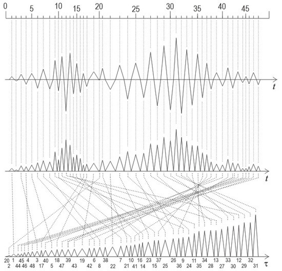
Figure 11.
The seismic waveform from Figure 2, approximated by triangles (up), is rectified (middle) and rearranged by increasing maximum amplitude (down). The indexing of spikes goes over all SFs, which is different from that in Figure 2, where separate numeration was applied to positive and negative SFs. The illegibility of the small font of integers around densly distributed spikes is alleviated using a non-linear ruler above the diagrams and vertical reference lines. At the bottom of the down diagram, mapped integers are shown individually.
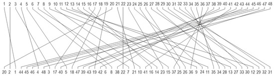
Now, the ordered sequence of rectified SFs is depicted in a bigraph called the absolute bigraph, shown in Figure 12.
Note the difference in assigning the SFs by integers in twin and absolute bigraphs.
The structure of the corresponding bipartite balanced absolute graph is presented in Figure 9. The mesh of edges reveals the stochastic structure of the sequence of SFs.
As stated in Methods, if the lower bigraph from Figure 6 is inverted (mirrored) to overlap it onto the upper one, to coincide nodes by their numbers, and slightly shifted one over the other to make their nodes visually distinguishable, one obtains a fused bigraph with 2N (input/output) nodes, and with 2N edges as well, connecting each pair of nodes (Figure 13). Now, this combined bigraph is of the same size (number of edges) as the absolute bigraph. The meshes of edges appear to be quite similar, and it will be interesting for further study.
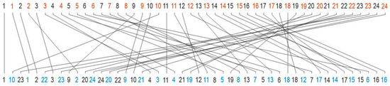
Figure 13.
When the down bigraph of the twin bigraph from Figure 6 is rotated (inverted), overlapped, and slightly shifted over the top one to the right (to make both bigraphs from the twin graph visually distinguishable), one gets a fused twin bigraph, very similar to the absolute bigraph, formerly produced by seismogram rectification. Close similarity between meshes of edges in these graphs can be noticed. Indexing of input and output nodes of the down bigraph is given in red and blue integers, respectively, to distinguish each other.
3.2. Seismogram Conversion—RQ-Envelope
In Section 2.4, in Figure 8, one can see a simple example of the R/RQ-envelope, given for better grasping the concept. Figure 14 presents a real case.
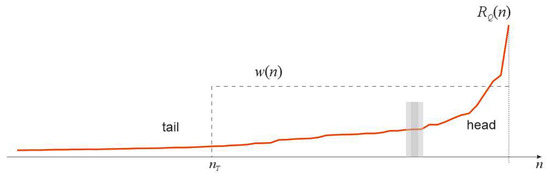
Figure 14.
The RQ-envelope of RSN70 SFERN (file taken from the PEER seismic database), drawn over only positive peaks. Two parts of the envelope are easily distinguished: the ‘head’, as non-stationary, and the ‘tail’, as gradually decreasing, almost monotonic. The gray bar indicates an arbitrarily positioned border between the two parts. The weighting function (window) w(n) is depicted by a dashed line to give the idea of tail trimming.
Different variability of the ‘head’ and the ‘tail’ is easily seen.
3.2.1. R/RQ-Envelope and Seismogram Variability
Figure 14 shows a real example of an RQ-envelope. It is obvious how the RQ-envelope reduces the intrinsic variability existing in seismograms. Variability is another name for randomness. Rearrangement of random SFs is actually a smoothing, averaging operation.
What one can see in Figure 14 is a gradually decreasing (monotonic) ‘tail’ and irregular ‘head’. This is natural since the tail is (usually) composed of many small SFs (i.e., Amaxs), while the head is composed of several large SFs (i.e., Amaxs). Therefore, it is more probable to find an SF among many other SFs whose peak amplitude is close enough to the peak amplitude of currently considered SFs. On the other hand, such probability is low for bigger or big SFs among a small number of big SFs. Because of that, one sees gradual change in the RQ-envelope along the tail and indented change along the head.
This means that the variability across the seismogram population is expected to be more prominent for heads of their RQ-envelopes, while the tails ‘stick together’.
Taking into account the heavy variability of seismogram duration, either expressed in time units (seconds) or by the number of SFs, namely the slight variability of the RQ tail corresponding to less significant SFs, gives the basis for applying the weighting function on the RQ-envelope to trim it to the prescribed length, so that the whole population of RQ-envelopes, i.e., the whole population of seismograms, can have the same size. The same can be said in terms of bigraph nodes, which will be explained later.
3.2.2. Examples of RQ-Envelope
In the following, several seismograms are represented by the RQ-envelope, which provides more complete insight into its main characteristics.
In addition to Figure 14, all Figure 15, Figure 16, Figure 17, Figure 18 and Figure 19, given below, confirm the previous impression that the RQ-envelope, and the R-envelope as well, is of similar shape over the whole population of seismograms.
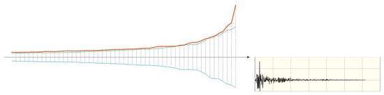
Figure 15.
RQ-envelope of RSN57 (San Fernando), taken from the PEER database, focal mechanism: Reverse, Horizontal-1 Component, contains both positive (red line) and negative (blue line) RQs. The modulo of RQ negative is depicted with a green line. At the right, just for quick visual reference, a small picture of seismogram waveform is inserted, with scale divisions: Dx=10s; Dy=0.2g (acceleration).
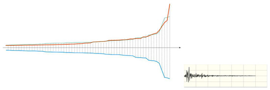
Figure 16.
RQ-envelope of seismogram of RSN70 (San Fernando), also taken from the PEER database, focal mechanism: Reverse, Horizontal-1 Component, already shown in Figure 14. Line colors have the same designation as in Figure 15. At the right, just for visual reference, a small picture of the seismogram waveform is inserted, with scale divisions: Dx = 10 s; Dy = 0.1 g (acceleration).
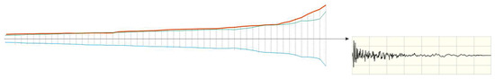
Figure 17.
RQ-envelope of seismogram of RSN88 (San Fernando), also taken from the PEER database, focal mechanism: Reverse, Horizontal-1 Component. Line colors as in Figure 15. At the right, a small picture of the seismogram waveform is inserted, with scale divisions: Dx = 5 s; Dy = 0.1 g.
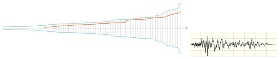
Figure 18.
RQ-envelope of seismogram of RSN286 (Irpinia), also taken from the PEER database, focal mechanism: Normal, Horizontal-1 Component. Line colors as in Figure 15. At the right, a small picture of the seismogram waveform is inserted, with scale divisions: Dx = 5 s; Dy = 0.05 g.
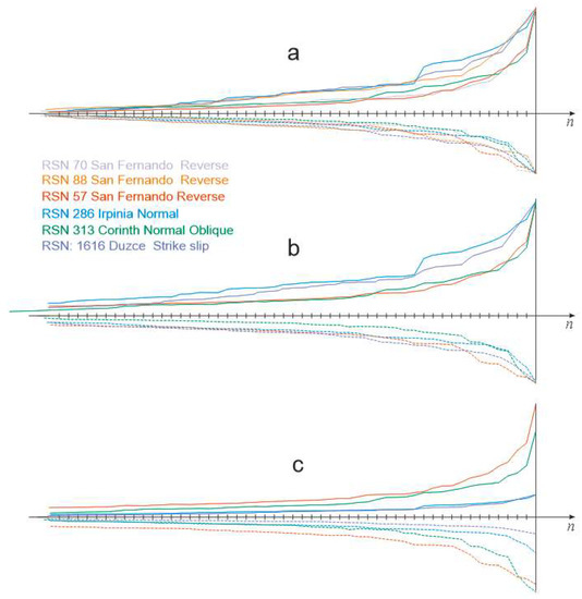
Figure 19.
For the list of seismograms, given between diagrams (a,b), an ensemble of RQ-envelopes, both positive (solid lines) and negative (dashed lines), is represented as the families of diagrams. All seismograms are taken from the PEER seismic database. Individual diagrams are normalized in certain aspects and overlapped. Colors of curves on diagrams correspond with colors of event names in the list. (c) The RQ-envelopes from indicated seismograms are only overlapped and justified by maximum amplitudes without normalization. (b) The four RQs from (c) are normalized by maximum amplitudes individually. (a) As in (b), where tails are additionally normalized by the smallest tail.
Moreover, it can be said that an invariant exists across the seismogram population. The authors expected such a conclusion, but not to that extent. If a certain, large level of seismogram variability remains in the head of the RQ-envelope, the tail is completely invariant. To further verify this inference, which might be an impression, although it was based on a few examples, more extensive research was carried out on a moderate sample of six seismograms.
Purposefully, the individual samples were miscellaneous and were not selected from one category defined in the database. The results are given in Figure 19.
The diagrams in Figure 19, particularly on (a), show a narrow variability of RQ; it seems too narrow to provide proper clustering.
3.2.3. Division Point between Head and Tail of RQ-Envelope
Figure 15, Figure 16 and Figure 17 show a very close symmetry of the RQ-envelope with respect to the n (or τ) axis. In other words, the envelopes RQ+ and RQ− are similar in shape.
The objective way, although one-parametric, to learn about their closeness is by calculating the difference
which is shown in Figure 20 for R(τ) of a typical distant seismogram. Again, one sees almost complete overlapping, closer for tails, less close for heads. Here might be found a criterion for a border separating the head and tail.
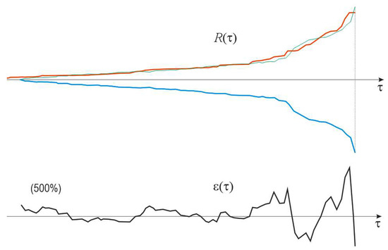
Figure 20.
Diagram ε(τ), magnified 500% for better clearness, shows the difference between positive (red solid line) and negative (blue solid line) envelopes of a seismogram, where the negative one is overlapped (green solid line) to be compared with the positive one. The change in overlapping measure along the t-axis gives the idea of where to put the separation point between the head and the tail of the R-envelope.
Having in mind all preceding diagrams and in the context of R(τ) symmetry, a general remark, even a recommendation, can be given; it suffices to analyze and process only the positive half of the seismogram, i.e., only positive SFs, thus saving of 50% of all necessary calculations in this approach.
Also, it makes the previous consideration about attaining a singular result in converting a seismogram into its bigraph slightly irrelevant. However, this remark can be regarded only in practical value, while the mathematical significance of seeking the singular product in the transformation process of a seismogram remains in full significance.
3.2.4. Measures of R/RQ-Envelope Variability
In converting seismograms into an RQ-envelope or bigraph, the transformation takes place and maps objects from the domain of raw seismograms into the domain of their representations, i.e., images, which are usually simpler than the originals and have less variability. In such cases, it is necessary to define a distance between images to accomplish grouping (clustering) more effectively.
For the case of R-envelope, the distance can be defined as:
which is, actually, the difference between two normalized R-envelopes, where the limits τ1 and τ2 are defined by R(τ)max and by weighting function w(τ) (see Figure 14).
A similar equation can be written for RQ(n) as well.
According to the previous interpretation, which is that the polygonal line defining the shape of R(τ) or of RQ(n) is essentially not the line but the string of numbers, the distance (17) can be rewritten as:
In both cases, one sees the importance of normalization since seismograms can significantly vary in maximum amplitude, while the waveform carries the most significant information and is the main factor in which seismograms differ from each other.
As a general remark, it should be stressed that the convention of the ordering direction of SFs, increasing maximum amplitudes from left to right adopted in this paper, is chosen quite by chance, with no objective reason. This means that the decreasing convention, from left to right, would be equivalent.
The pronounced difference in the shape of the head and the tail in the RQ-envelope inspired the idea to separately measure the distance for both of them.
3.3. Bigraph Variability and Issue of Measure
The RQ-envelope and the bigraph are considered equivalent representations of seismograms. How, then, can we explain the issue of the variability of the bigraph?
It is easy to notice bundles in the mesh of edges within the bigraph. Moreover, it is easy to identify bundles corresponding to respective groups of SFs just by comparing the output nodes of the bigraph with the shape of the RQ-envelope. It is easy to grasp this idea by comparing Figure 3 and Figure 4. There, it is easy to select the main bundle of edges, respective to SFs (i.e., SF(A)s, or Amaxs), which form the ‘head’ of the RQ-envelope. There are also other bundles that can be identified.
Relying on the claimed equivalence between the bigraph and the RQ-envelope, it is easy to see that the RQmax corresponds to the biggest SF/SF(A) or to the rightmost output node nK in the bigraph (according to the convention of increasing values of SFs).
The edge eK, connected to the node nK, designates the mapping of the largest SF/SF(A) and can be named as the structural axis of bigraph (spine, backbone), a reference for considering other edges or bundles of edges.
Obviously, the meaning of these terms depends on the bigraph geometry, which, in this paper, is chosen to be a two-row structure with connecting lines between.
Remembering the previous double indexing of output nodes, positional (mapped) and regular (see Figure 9), it is easy to measure each edge by simply subtracting the correspondent indices, for example:
This means that the mapping distance of the main node (max SF), which is labeled by index 16 (defining its position in input nodes), is translated (mapped) to position 24 (output nodes), which equals 8 units of displacement.
md(nK) = md(24) = 24 − 16 = 8
Similarly, e.g., input node 7, which is mapped to position 20 of the output index string, which makes md(20) = 20 − 7 = 13 units of displacement.
For the given bigraph geometry, its height is Hb, and the mapping distance yields the edge slope:
around which are arranged edges with similar slopes, making the primary bundles the main structural element of the bigraph (in its mesh).
α(nK) = α(24) = arcsin(Hb/md(24))
In that way, a relationship is established between the head in the diagram of RQ and the primary bundle in the bigraph mesh. In a similar way, one can define secondary bundles.
Formatting of Bigraps
One dimension of seismogram variability is its duration, which, when transferred into an RQ or bigraph, means the number of SFs or the bigraph size (number of nodes). Even a group of earthquakes defined by a certain set of grouping criteria shows heavy variability and prevents clustering.
There are two proposals to equalize variable lengths of seismograms.
Extension of bigraph by empty complement—It is well known from number theory and binary coding that, e.g., 011 = 00000011. Applying this simple idea to bipartite graphs, an empty bigraph is added to the current (actual) bigraph to attain the prescribed size. In other words:
which one reads out as the size (G) of the extended bigraf is the sum of the sizes of the actual bigraf and its empty complement bigraph to attain a prescribed size (see Figure 21), constant for all bigraphs.
#(BGE(k)) = #(BG(k)) + #(E(k)) = G, ∀k
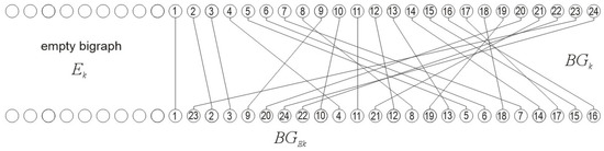
Figure 21.
To illustrate the concept of the empty graph, the simple graph from Figure 4 is used, which is extended by an empty graph to the prescribed size. Note that the direction of extension goes along the least significant nodes (SFs).
Another parallel with the empty bigraph can be found in the set theory, with the empty set, but there are significant differences. The empty set has nothing in it but possesses only its existence, pointing to the fact that the set is a frame, and after that, it becomes a real set by containing certain elements.
The empty bigraph is not totally empty: it contains nodes but not the edges between them. Let us note that the Gilbert model of the random graph contains one realization in its statistical ensemble, which is a graph with no edges, similar in the sense of the defined concept of an empty graph [27].
Weighting function—In seismic science, researchers need complete seismograms to study an earthquake’s whole background, processes in source, and propagation afterward. In other areas of research and engineering, often there is no need for the whole waveform, but just for certain segments (e.g., seismic civil engineering). By applying the proper weighting function (also known as the window function from digital signal processing), one can extract the most important segment on purpose and reduce the variability across the seismogram sample and, hence, of respective bigraphs.
Note that the simplest, rectangular weighting function is applied since the application of any monotonic one would convert the original bigraph, which is simple (no weighted nodes or edges), into a weighted graph, which would be more complicated for analysis [29].
The weighting function is positioned with respect to the highest SFs (Figure 22) so that it encompasses the most significant SFs and cuts off the tail of less significant ones. Of course, the question of where to place the cut has to be considered.
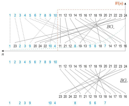
Figure 22.
Bigraph BG+ from Figure 4, is truncated by rectangular weighted function (window, depicted by dashed orange line) W(n) so that less significant SFs are eliminated from describing the positive part of the seismogram. The dashed green line curve on the W(n) diagram indicates the increasing direction of the ordered sequence of positive SFs (the largest SFs are at the right end). Dashed black lines and blue numbers depict discarded edges and nodes, respectively. After that, the remaining nodes and respective edges are rearranged to give a compact bigraph BG+.
A very important additional effect of the weighting function application appears. Since the output nodes are randomly interleaved, the edges in the whole mesh of bigraph, which correspond to cut-off input nodes (i.e., insignificant SFs), and form a sub mesh, will disappear, so the remaining bigraph should be compacted, which involves rearrangement of residual bigraphs (Figure 22). The compacting changes the mesh structure. It will be very interesting to compare the edge mesh of original and trimmed bigraphs.
On the contrary, for seismograms of prominently impulse character, i.e., of short duration, in order to avoid such specific cases to determine the trimming length of the predominant rest of the longer seismograms in the population, the concept of the empty bigraph may be of help.
3.4. Examples of Seismogram Combined Representation by Bigraph and RQ-Envelope
The bigraph and the RQ-envelope create a complementary representation of a seismogram. In the following, a few examples are given and briefly interpreted. All examples are taken from the PEER seismic database except the last one.
3.4.1. RQ-Envelope and Bigraph of Seismogram RSN1616
This example is interesting because of the fact that complex waveforms of EFs/SFs compose the seismogram, so that the interesting results might be expected. It seems to be obvious from its waveform, given at the top of Figure 23, but the RQ-envelope shows pretty calm decreasing.
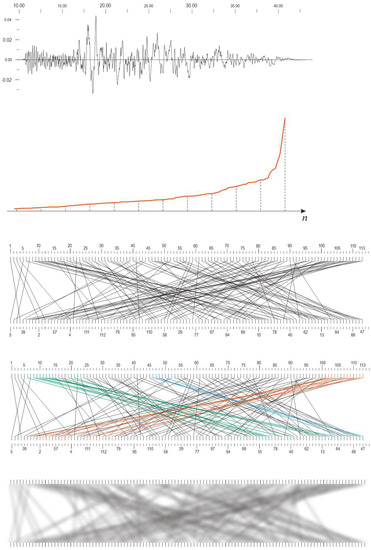
Figure 23.
(from (top)–(down)) Representative seismogram (RSN 1616 Duzce (Düzce) 1999, Turkey, Lamont 362), containing plenty of different SF shapes, with main parameters: D5–75 14.6 s, D5–95 20.5 s, Mag 7.14, Strike-Slip, RJB 23.41 km, Rrup 23.41 km; file used DUZCE_362-N.AT2, Horizontal-1 Component time series). (next) RQ-envelope for positive SFs (113 points). (next) Bigraph only for positive SFs (black and white). (next) Bigraph only for positive SFs (colored, to indicate main structural bundles): blue edges form the main (primary) bundle of bigraph, the green ones form a secondary bundle, while the red bundle is of the least significance. (next) Bigraph just for positive SFs (black and white, blurred with Gaussian blur to better indicate all structural bundles in the edge mesh). Numeric labeling of input (up) and output (down) nodes are, for visual simplicity, indicated by enumerated scales, where the upper sequence of integers is regular (1, 2, 3, 4, 5, 6, …, 120), while the down random one is determined by edges. The size of the bigraph is 113.
The number of nodes in the bigraph, 113 in total, corresponds to the number of significant SFs. The bigraph mesh of edges shows characteristic bundles.
It is important to note that blurred diagram is intentionally blurred to emphasize the bundles of edges, and in such shadowy manner to reveal skeleton of bigraph mesh.
3.4.2. RQ-Envelope and Bigraph of Seismogram RSN286
This example of seismogram is impulse-like waveform, with asymmetry in negative main amplitudes. Its RQ-envelope (Figure 24) shows perturbation of the head.
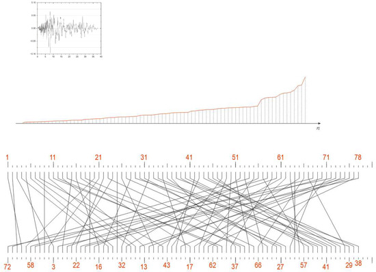
Figure 24.
Seismogram RSN286. Insert shows its waveform for reference. RQ is distinguished by specific head shape. The structural content of the bigraph shows uniform crossing of edges within broad area of mesh.
The bigraph mesh seems to be pretty uniform, without prominent bundles (Figure 24).
3.4.3. RQ-Envelope and Bigraph of Seismogram RSN313
This example seems pretty similar to the previous one, with still more prominent pulse nature. Again there are prominent negative spikes. The RQ-envelope is almost regular along its head (Figure 25).
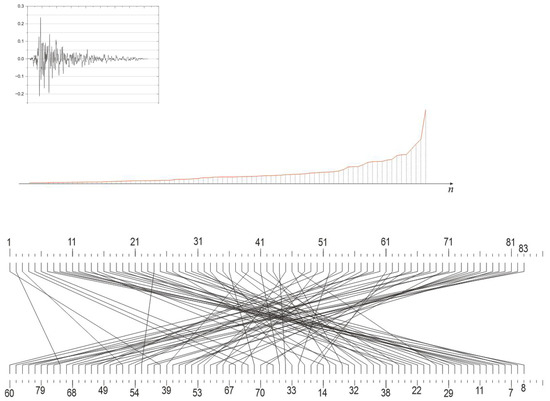
Figure 25.
Seismogram RSN313. Insert shows its waveform for reference. Structural content of the bigraph shows almost only two main bundles, sharply covering big and small spikes.
However, the bigraph is of very specific structure, showing two main bundles, almost divided into two separated halves (Figure 24).
3.4.4. RQ-Envelope and Bigraph of Typical Distant Seismogram
Distant seismograms are typically characterized by resonances, and by quasi periodicity, of the random form. As can be seen on Figure 26, the RQ-envelope is generally monotonic, with ripples on the head. As for the bigraph, its mesh is almost uniformly intertwined, in a similar way for positive and negative spikes (Figure 26).
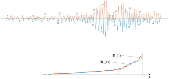
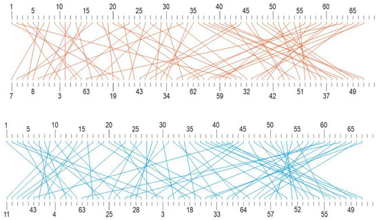
Figure 26.
(from (top)–(down)) An example of a distant seismogram: SFs are labeled by positive integers, separately for positive (red) and negative (blue) SFs. For better legibility of SF indexing, same indices are given in bigger font size, while the others can be easily identified by enumerating ‘points’ (i.e., indices in small size font) between them. (next) Both R(τ) envelopes, for positive and negative SFs. (next) Bigraph for positive SFs. (next) Bigraph for negative SFs.
The RQ part of the complement RQ-BG, as the result of said transform of the seismogram, evidently reduces original variability to a narrow interval. It is so narrow that there seemingly is not enough room for effective clustering of seismogram images. This claim will be verified on a sample of seismograms of sufficient size, which would provide well-grounded statistical inference. This paper had no intention to go that deep into this issue to avoid its unacceptable volume.
Although both the RQ and bigraph are the result of SFs ordering, the RQ is a somewhat closed image of the seismogram, while the bigraph is more open, having more degrees of freedom for the clustering process. Otherwise, the bigraph possesses not only a wider interval for clustering with respect to RQ, but it has the frame for that, provided by several structural elements, bundles, and elements within bundles.
4. Discussion
The primary intention of this paper was limited to only introducing the new concept and considering its features in the frame of seismogram interpretation, processing, and, finally, more effective clustering. Some quantitative and qualitative results are given, which contain assessments of issues of reduced variability and clustering. The exact verification of these issues, in addition to a comprehensive presentation of the many items in this paper, would lead to excessive volume; therefore, it is left for the next research.
Seismogram variability and issue of grouping—An earthquake is a very complex random phenomenon, i.e., a very complex random entity with immense variability, which imposes difficulties in grouping (clustering) and database organization.
Typically, grouping (clustering) criteria (parameters) usually include fault (focal mechanism), distance, magnitude, duration (D5–95(s)), Rjb (Joyner–Boore distance), Arias intensity, event name, station name, year, etc. [18]. These are general criteria whose generality confirms said difficulties.
The fault mechanism could serve as a basic classification factor. However, earthquakes affect the surrounding areas, bringing propagation effects into seismograms recorded at certain sites. This is easily seen in, e.g., the PEER database, which is organized according to general criteria despite the fact that it is the result of tremendous accumulated experience and knowledge.
In dealing with a database, one enters parameters for a certain group (class) and can work with any of the presented seismic events (i.e., earthquake), either in the form of its seismogram (time series) or its spectrum. Selecting an individual event from the database by its name is a trivial operation and not concerned with its organization.
It is interesting to notice that the spectrum, as an ordered and more compact image of the seismogram with less variability, is only an entity added to the seismogram, but, as such, not a factor that can be used for database organization, i.e., not a factor but the object of grouping.
The problem of clustering objects that are difficult to cluster is usually solved by converting one object into another using a mathematical operation called transform, mapping it from the original domain into the domain of the object’s images, which are now easier to cluster.
This paper proposes an approach to transforming a seismogram into a combination of an RQ-envelope and bigraph, which, then, deserves the name transform.
More about the variability of RQ-envelope and bigraph—Previously, RQ variability was thoroughly considered, and its measure was defined. It can serve as a distance in certain topological spaces, which is the basis for the criterion of clustering (grouping). The variability of the head and the tail in the RQ-envelope is quite different (see Figure 14).
For the shape of the RQ-envelope, one can even speak of it as invariant. More precisely, the head of the RQ is less invariant than the tail of the RQ, which is inherently invariant, so it is possible to divide the RQ into two parts and consider their variability in different ways or even measure their variability according to different criteria. In a practical way, the issue of RQ variability can be brought down to the head variability.
As for bigraph variability, the measure of distance relies on primary and secondary bundles, angle, and number of edges per bundle.
RQ as invariant and redundancy in seismogram—The form of the RQ and convergence in its ensemble apparently suggest the existence of a kind of invariant. Moreover, they suggest redundancy in seismograms as well since all seismograms addressed in this paper show very close similarity between their RQs. This means that each seismogram contains plenty of redundant information. It is well known that the alternating fluctuation along the waveform is the main cause of redundancy through strong local correlation of alternating amplitudes.
In this regard, an important fact should be underlined: the RQ is the result of the ordering of SFs by peak amplitudes. This means that in the ordering procedure, all local correlative interrelations that provide seismogram redundancy are disrupted. Then, one would expect redundancy to decrease, but it is increased. The explanation of this paradox is simple: the ordering means putting the most similar SFs one next to the other (which are now closer by peak amplitude), which now means the appearance of additional correlation. This is an interesting effect and deserves further analysis.
Equivalence of R-envelope and bigraph—This issue has been discussed extensively so far. Here, we will add just a few essential remarks.
Instead of the term ‘equivalence’, it might be more appropriate to qualify the R-envelope and bigraph as complementary characteristics, although their equivalence cannot be disputed.
The R- and RQ-envelopes contain information on maximum amplitudes of SFs, giving the amplitude content of the seismogram waveform.
If one assumes regular indexing along the abscissa, then the complete information about the mapping structure is lost. However, if one adds positional indexing, then the complete mapping is known, and, actually, the complete bigraph is given below the abscissa (Figure 8 and Figure 9). Thus, the R- or RQ-envelope with positional indexing contains the complete bigraph. On the other hand, the bigraph, without any additions, directly by its structure, by nodes and mesh of edges, reflects the general structure of the seismogram but without data about maximum amplitudes. This is for the case of a simple bigraph with no weights in nodes and edges. In brief, one can say that the bigraph is more internal, while the R/RQ-envelope is a more external representation of the seismogram.
Main part of the seismogram—There is an additional distinction in the previous concept. The main part of a seismogram is the one containing significant SFs, i.e., all SFs that are large, which mostly cause significant seismic effects on the built environment. An ordering operation gathers these SFs together, whatever their disposition throughout the seismogram, so that the ordered seismogram is a monotonic object where SFs gradually increase or decrease, depending on the ordering convention (starting from the largest or from the smallest SF). The main part of the rearranged seismogram contains the SFs that are the most important for seismic effects (magnitude, delivered energy, inflicted damage, influence on structures, etc.). The long decreasing tail of the ordered seismogram stems from the tail, which is of secondary influence and significance. Therefore, the ordering makes more explicit the issue of what part of the tail is to be recorded or where to terminate its recording prior to it sinking into seismic noise.
One should be careful when considering the main part of the seismogram. The rearrangement operation gathers all the prominent SFs in one place, sometimes from different areas of the seismogram, so it may produce the impression that they act together. In addition, the SFs are gathered one-sided, positive, negative, or both, with the seismogram rectified. This means they seemingly act in one direction, but the essential capability to influence the built environment and cause damage is its vibratory (alternating) behavior when two maximum opposite SFs, as a part of the most prominent EF, run over the structures.
It is interesting to note that the head of the RQ-envelope corresponds with the main part.
Does the transform produce a simple or weighted bigraph?—This paper is written under the assumption that all forms of bigraphs that result from transform are simple, which means that they are not directed nor weighted (the nodes and edges are simple).
Let us remember that the ordering operation rearranges SFs; therefore, the significant ones are separated from less significant or insignificant ones. In other words, the significance of SFs rises along the ordered sequence. Since the SFs are transposed into nodes of a bigraph, it is quite natural to consider input nodes as weighted, different from each other. Similarly, an edge that connects significant (input and output) nodes (read: SF with bigger maximum amplitude) cannot be considered equal to the edge connecting insignificant edges. Therefore, the answer to the title question is obvious. Analysis of weighted bigraphs is more complex than that of simple ones. We followed an implicit assumption in this paper, which was to treat all forms of bigraphs introduced in the paper as simple, as our intention was to present these fundamental concepts in a clear context. In further research, it will be natural to consider weighted bigraphs.
Bipartite graph randomness—In the Introduction, we mentioned deterministic and random bipartite graphs. The first show all existing relations (edges) between input and output nodes. It is seemingly the same in the case of a random graph—one sees the firm structure of edges between nodes in such a graph. Actually, a random graph shows possible (potential) edges between nodes.
This means, in the case of a (deterministic) conventional graph, the actual graph is the only one, while in the second case, the considered graph is just one of many possible realizations, creating a whole statistical ensemble in which any of its elements is a graph with a firm structure, but slightly different from the others. Each ‘tossing’ (trial) of the potential random graph produces a different realization—a graph with a firm structure.
EFs/SFs and wavelets—There is an apparent similarity between the concept of EF/SF and wavelets. How, otherwise, to call these ‘wavelets’ when they are small chunks of a complex waveform, a seismogram in this case?
The authors deliberately decided not to use the term wavelet in this case.
The term wavelet can have two associations: as a small wave (impulse) and as a mathematical object. What is more, these associations can be mixed, and one can complain about borrowing that name for a new concept.
The concept of EF/SF truly reminds us of wavelets, which begs for a comparison of these two approaches to seismogram description. Wavelets are particularly suitable for localized signals and random transients; a typical example is the seismic signal represented by a seismogram.
Regarding the comparison between the concept of EF/SF and wavelets, there are essential differences. The wavelets (of a certain type) represent a system of similar elementary waveforms and impulses, a kind of offspring originating from a generative function, the so-called mother function. They form the basis within which a signal is to be decomposed. It is quite similar to the FT, where a sinusoid is a generative function, the function of a parameter, which can create a set of harmonics, a basis for signal decomposition.
As for the concept of EF/SF introduced in this paper, it is impossible to create a basis because they are not only parametrically interrelated but are of random shape, i.e., the SFs do not have shape similarity. In addition, SFs are not ‘wavelets’ that are applied to the waveform from outside as wavelets do, they come from inside; moreover, they are parts of the waveform they intend to analyze.
Speaking of wavelet transform, spectral descriptions of seismograms are widely used in various areas related to seismic effects and their consequences. The prominent place of spectrum in seismic databases confirms its significance and practical applicability. However, the Fourier transform (FT), with its numerical derivatives (STFT, DFT, and FFT), still dominates the spectral world, while the WT gradually builds its place in it.
5. Conclusions
The theme of the paper proved to be quite interdisciplinary.
The authors’ ambition was not to make a complete discovery and a new database but, for the present, only to point out the direction of possible solutions and to propose characteristics that promise solutions.
The proposed characteristics, the RQ-envelope and bipartite graph, certainly reduced the variability of seismograms.
As for the RQ, the extent of variability narrowing makes one think that the RQ is very close to being an invariant of the seismogram population. This finding deserves thorough further research.
On the other hand, the narrow range in which the RQ-envelope varies makes it a questionable basis for clustering of the seismogram population.
The bigraph, in comparison to the RQ, also attains narrowed variability but within a domain having a few degrees of freedom. The bigraph goes deeply into the structure of the seismogram, describing its waveform in a more thorough manner through the system of edge bundles. The authors’ assessment is that it provides a wider basis for clustering with respect to existing one-parametric criteria.
This transform opens the door for defining various characteristics of seismograms.
The presented approach is obviously not limited only to seismograms but can be applied to all similar stochastic processes.
Author Contributions
Conceptualization, R.B.; Resources, R.B. and L.B.; Data curation, R.B. and L.B.; Formal analysis, R.B.; Supervision, R.B.; Investigation, R.B.; Visualization, R.B., Methodology, R.B. and L.B.; Writing—original draft, R.B. All authors have read and agreed to the published version of the manuscript.
Funding
This research received no external funding.
Institutional Review Board Statement
Not applicable.
Informed Consent Statement
Not applicable.
Data Availability Statement
Not applicable.
Acknowledgments
Using the seismograms from the PEER Ground Motion Database greatly contributed to our research.
Conflicts of Interest
The authors declare no conflict of interest.
References
- Bormann, P. (Ed.) IASPEI New Manual of Seismological Observatory Practice; GFZ German Research Centre for Geosciences: Potsdam, Germany, 2012; Available online: http://nmsop.gfz-potsdam.de (accessed on 10 September 2023). [CrossRef]
- To, G.F.; Schubert, G. (Eds.) Treatise on Geophysics, 1st ed.; 11 Volumes Set; Elsevier: Amsterdam, The Netherlands, 2007; 6054p, ISBN 10:0444519289. Available online: https://www.geokniga.org/bookfiles/geokniga-treatise-geophysics.pdf (accessed on 15 July 2023).
- Havskov, J.; Ottemöller, L. Processing Earthquake Data, October 2009. Available online: https://www.geo.uib.no/seismo/SOFTWARE/DOCUMENTATION/processing_earthquake_data.pdf (accessed on 22 August 2023).
- GFZ, Seismic Hazard and Risk Dynamics, Seismic Hazard Assessment for the D-A-CH countries. Available online: https://www.gfz-potsdam.de/en/section/seismic-hazard-and-risk-dynamics/projects/previous-projects/probabilistic-seismic-hazard-assessments/d-a-ch-seismic-hazard-for-the-d-a-ch-countries-germany-austria-switzerland (accessed on 6 September 2023).
- Grünthal, G.; Mayer-Rosa, D.; Lenhardt, W. Joint strategy for seismic hazard assessment; application for Austria, Germany and Switzerland. In Proceedings of the 21st General Assembly of the International Union of Geodesy and Geophysics (IUGG), Boulder, CO, USA, 2–14 July 1995. B 404. [Google Scholar]
- Spence, R.; So, E.; Jenny, S.; Castella, H.; Ewald, M.; Booth, E. The Global Earthquake Vulnerability Estimation System (GEVES): An approach for earthquake risk assessment for insurance applications. Bull. Earthq. Eng. 2008, 6, 463–483. [Google Scholar] [CrossRef]
- Jayaram, N.; Shome, N.; Rahnama, M. Development of earthquake vulnerability functions for tall buildings. Earthq. Eng. Struct. Dyn. 2012, 41, 1495–1514. [Google Scholar] [CrossRef]
- Preciado, A.; Ramirez-Gaytan, A.; Salido-Ruiz, R.A.; Caro-Becerra, J.L.; Lujan-Godinez, R. Earthquake risk assessment methods of unreinforced masonry structures: Hazard and vulnerability. Earthquakes Struct. 2015, 9, 719–733. [Google Scholar] [CrossRef]
- Gaxiola-Camacho, J.R.; Azizsoltani, H.; Villegas-Mercado, F.J.; Haldar, A. A novel reliability technique for implementation of Performance-Based Seismic Design of structures. Eng. Struct. 2017, 142, 137–147. [Google Scholar] [CrossRef]
- Maio, R.; Ferreira, T.M.; Vicente, R. A critical discussion on the earthquake risk mitigation of urban cultural heritage assets. Int. J. Disaster Risk Reduct. 2018, 27, 239–247. [Google Scholar] [CrossRef]
- Shadmaan, S.; Islam, A.I. Estimation of earthquake vulnerability by using analytical hierarchy process. Nat. Hazards Res. 2021, 1, 153–160. [Google Scholar] [CrossRef]
- Dowrick, D. Earthquake Resistant Design and Risk Reduction, 2nd ed.; Wiley: Chichester, UK, 2009; ISBN 13:9780470778159. [Google Scholar]
- Duggal, S.K. Earthquake-Resistant Design of Structures, 2nd ed.; Oxford University Press India: Noida, India, 2013; Available online: https://www.technicalbookspdf.com/earthquake-resistant-design-of-structures-2nd-edition/ (accessed on 10 September 2023).
- FEMA Earthquake-Resistant Design Concepts, An Introduction to the NEHRP Recommended Seismic Provisions for New Buildings and Other Structures, FEMA P-749/December 2010; National Institute of Building Sciences Building Seismic Safety Council: Washington, DC, USA, 2010. Available online: https://www.fema.gov/sites/default/files/2020-07/fema_earthquake-resistant-design-concepts_p-749.pdf (accessed on 2 September 2023).
- Sucuoğlu, H.; Akkar, S. Basic Earthquake Engineering-From Seismology to Analysis and Design; Springer: Cham, Switzerland, 2014. [Google Scholar] [CrossRef]
- Moshou, A.; Konstantaras, A.; Argyrakis, P.; Petrakis, N.S.; Kapetanakis, T.N.; Vardiambasis, I.O. Data Management and Processing in Seismology: An Application of Big Data Analysis for the Doublet Earthquake of 2021, 03 March, Elassona, Central Greece. Appl. Sci. 2022, 12, 7446. [Google Scholar] [CrossRef]
- Lindup, G.; Sharpe, R.; Holm, S.; Jarman, S.; Sinclair, R.; Bloomer, A.; Tsamandakis, E.; Smart, C. Practice Note 19 Seismic Resistance of Pressure Equipment and Its Supports; engineering New Zealand: Wellington, New Zealand, 2019; ISSN 1176-0907. Version 5; Available online: https://d2rjvl4n5h2b61.cloudfront.net/media/documents/PN19-SeismicResistancePressureEquipment_V5-2019.pdf (accessed on 10 September 2023).
- PEER. PEER Ground Motion Database. 2022. Available online: https://ngawest2.berkeley.edu/spectras/new?sourceDb_flag=1 (accessed on 9 September 2023).
- Scasserra, G.; Stewart, J.P.; Kayen, R.E.; Lanzo, G. Database for Earthquake Strong Motion Studies in Italy. J. Earthq. Eng. 2009, 13, 852–881. [Google Scholar] [CrossRef]
- Yuan, X.; Wang, X.; Guo, J.; Dou, A.; Ding, X. Design and realization of RS application system for earthquake emergency based on digital earth. In IOP Conference Series: Earth and Environmental Science, Proceedings of theDigital Earth Summit, Beijing, China, 7–8 July 2016; IOP Publishing Ltd.: Bristol, UK, 2016; Volume 46, p. 012037. [Google Scholar] [CrossRef]
- USGS National Earthquake Information Center (NEIC), Earthquake Hazards Program. Available online: https://www.usgs.gov/programs/earthquake-hazards/seismogram-displays (accessed on 6 September 2023).
- Bollobash, B. Random Graphs; Cambridge University Press: Cambridge, UK, 2001; M08 30. [Google Scholar]
- Barabási, A.-L. Network Science. Available online: http://networksciencebook.com/ (accessed on 10 September 2023).
- Erdös, P.; Rényi, A. On the Evolution of Random Graphs; The Mathematical Institute of the Hungarian Academy of Sciences: Budapest, Hungary, 1960; Volume 5, pp. 17–61. [Google Scholar]
- Gilbert, E.N. Random graphs. Ann. Math. Stat. 1959, 30, 1141–1144. Available online: https://www.stat.cmu.edu/~brian/780/bibliography/09%20Other%20Models/Gilbert%20-%201959%20-%20Random%20graphs.pdf (accessed on 10 September 2023). [CrossRef]
- Newman, M. Networks: An Introduction; OUP: Oxford, UK, 2010; M03 25. [Google Scholar]
- Dorogovtsev, S.N. Lectures on Complex Networks; Clarendon Press: Oxford, UK, 2010; Available online: https://sweet.ua.pt/sdorogov/dorogovtsev_lectures_first_pages.pdf (accessed on 10 September 2023).
- Dorogovtsev, S.N.; Mendes, J. The Shortest Part to Complex Networks. July 2004. Available online: https://arxiv.org/abs/cond-mat/0404593 (accessed on 10 September 2023).
- Clauset, A. Three Lectures on Networks. 2022. Available online: https://aaronclauset.github.io/slides/Clauset_2022_CSSS_IntroNetworks_1.pdf (accessed on 10 September 2023).
- Sayama, H.; Cramer, C.; Porter, M.A.; Sheetz, L.; Uzzo, S. What are essential concepts about networks? J. Complex Netw. 2015, 4, 457–474. [Google Scholar] [CrossRef]
- Asratian, A.S.; Denley, T.M.J.; Häggkvist, R. Bipartite Graphs and Their Applications; Cambridge University Press: Cambridge, UK, 1998. [Google Scholar]
- Pavlopoulos, G.A.; Kontou, P.I.; Pavlopoulou, A.; Bouyioukos, C.; Markou, E.; Bagos, P.G. Bipartite graphs in systems biology and medicine: A survey of methods and applications. GigaScience 2018, 7, 1–31. [Google Scholar] [CrossRef] [PubMed]
- Cvetković, D. Applications of Graph Spectra: An Introduction to the Literature. Available online: https://elib.mi.sanu.ac.rs/files/journals/zr/21/n021p007.pdf (accessed on 10 September 2023).
- Brouwer, A.; Haemers, W. Spectra of Graphs, Monograph, 1 February 2011. Available online: https://www.win.tue.nl/~aeb/2WF02/spectra.pdf (accessed on 10 September 2023).
- Han, J.; Kamber, M. Data Mining: Concepts and Techniques, 2nd ed.; Elsevier: Amsterdam, The Netherlands, 2006. [Google Scholar]
- Joshi, K.D. Introduction to General Topology; New Age International: New Delhi, India, 1983; reprint 2004. [Google Scholar]
Disclaimer/Publisher’s Note: The statements, opinions and data contained in all publications are solely those of the individual author(s) and contributor(s) and not of MDPI and/or the editor(s). MDPI and/or the editor(s) disclaim responsibility for any injury to people or property resulting from any ideas, methods, instructions or products referred to in the content. |
© 2023 by the authors. Licensee MDPI, Basel, Switzerland. This article is an open access article distributed under the terms and conditions of the Creative Commons Attribution (CC BY) license (https://creativecommons.org/licenses/by/4.0/).