Abstract
An Electric Solar Wind Sail (E-sail) is a propellantless propulsion concept that extracts momentum from the high-speed solar wind stream to generate thrust. This paper investigates the performance of such a propulsion system in obtaining the transition from a prograde to a retrograde motion. The spacecraft is assumed to initially trace a circular heliocentric orbit of given radius. This particular trajectory, referred to as Circular Orbit Flip Trajectory (COFT), is analyzed in a two-dimensional mission scenario, by exploiting the capability of a medium-high performance E-sail to change the spacecraft angular momentum vector during its motion in the interplanetary space. More precisely, the paper describes a procedure to evaluate the E-sail optimal performance in a set of COFTs, by calculating their minimum flight times as a function of the sail reference propulsive acceleration. It is shown that a two-dimensional COFT can be generated by means of a simple steering law in which the E-sail nominal plane has a nearly fixed attitude with respect to an orbital reference system, for most of the time interval of the interplanetary transfer.
1. Introduction
A plane change maneuver, i.e., a maneuver that changes the orbital inclination of a Keplerian orbit while keeping the semimajor axis and eccentricity (i.e., both its shape and size) unchanged [1], is usually considered to be one of the most demanding maneuvers in astrodynamics from the standpoint of velocity change and, therefore, propellant expenditure [2]. A possible solution to perform such an orbital maneuver is given by the use of a propellantless propulsion system, such as a (photonic) solar sail [3,4,5] or an Electric Solar Wind Sail (E-sail) [6], which exploit either the solar radiation pressure (solar sail case) or the solar wind momentum flux (E-sail case) to generate a propulsive acceleration.
The solar sail capabilities in a plane change maneuver of a circular heliocentric orbit have been analyzed by the authors [7] as a special case of a more general orbit-to-orbit interplanetary transfer between two mutually inclined circular trajectories. A plane change maneuver with an E-sail-based spacecraft has not yet been investigated and is not even the goal of this work because, in this regard, a detailed study is left for future research. Instead, the aim of this paper is to analyze a more specific mission scenario in which the orbital inclination of a given heliocentric Keplerian orbit is changed by exactly 180 degrees. In other terms, this particular plane change maneuver allows the spacecraft to invert its direction of rotation around the Sun, thus obtaining a sort of artificial (thrust-induced) ‘orbit flip mechanism’ [8,9,10,11], which preserves the shape and the dimension of the original trajectory. More precisely, the focus of this study is on the analysis of the orbit flip mechanism of a circular heliocentric orbit of assigned radius, by means of a two-dimensional propelled trajectory coplanar to the initial circular orbit. Such a COFT is obtained by using the propulsive acceleration given by an E-sail propulsion system.
An E-sail is a propellantless thruster concept proposed by Pekka Janhunen [12,13,14,15] at the beginning of this century. Such a propulsion system uses a number of conducting tethers [16,17,18] to deflect the solar wind and obtain a thrust in the interplanetary space [18,19,20]. The E-sail thrust vector can be steered [21,22,23] by suitably changing the sail attitude with respect to the solar wind stream direction [24,25]. The main characteristics of the E-sail concept are thoroughly illustrated in a recent review paper [6], while an interesting collection of papers on E-sail mission applications is reported in a special issue of the companion Aerospace journal (The Aerospace special issue named “Advances in CubeSat Sails and Tethers” can be found at the URL https://www.mdpi.com/journal/aerospace/special_issues/2319OV36DR, accessed on 23 August 2023).
The new features of this work are essentially two. The first one concerns the study of the COFT from an optimal point of view, using a general mathematical model that can be employed in a wide range of mission scenarios. In fact, the proposed model provides a set of graphs that allow the reader to quickly estimate the E-sail performance in a COFT without the need of numerical simulations. The optimization process also points out that a generic COFT can be thought of as a special case of Vulpetti H-reversal trajectory, the main features of which are illustrated in the review by Zeng et al. [26]. The second and most important contribution of this work lies in a particular shape of the COFTs, which has been identified during the numerical study of the trajectories. In fact, the optimization process has shown that there exists a family of COFTs that presents a close passage near the Sun and a zero magnitude of the inertial velocity in correspondence of the aphelion point. This particular feature of COFTs had not been discovered during previous studies of heliocentric trajectories with H-reversal points. In this sense, the utility of the results of this work can be considered more general than the simple application to a mission case involving an orbit flip maneuver.
The paper is organized as a follows. Section 2 describes the mission scenario and illustrates the mathematical model used to obtain the COFT as a function of the propulsive performance of the E-sail. The core of the paper is Section 3, which highlights the characteristics of the COFTs obtained through the optimization process. In particular, Section 3 illustrates two possible shapes of the optimal trajectory. Finally, Section 4 critically analyzes the obtained results and proposes possible extensions of this work.
2. Problem Description and Mathematical Approach
Consider a heliocentric, two-dimensional mission scenario in which a spacecraft initially (i.e., at time ) follows a circular orbit of assigned radius around the Sun. Note that the mathematical model for an elliptic parking orbit can be obtained by paralleling the procedure described in the recent Ref. [27]. The spacecraft primary propulsion system is an E-sail with an assigned value of characteristic acceleration , which is defined as the maximum magnitude of the E-sail propulsive acceleration when the distance from the Sun is . In particular, according to the mathematical model proposed by Huo et al. [28], the analytical expression of is
where is a dimensionless switching parameter that models the thruster operating mode (either on, when , or off, when ), is the Sun-spacecraft (or radial) unit vector, r is the Sun-spacecraft distance, and is the unit vector normal to the sail nominal plane (i.e., the plane that nominally contains the conducting tethers) such that . In particular, if the E-sail attitude is fixed with respect to an orbital reference frame, then the magnitude of is inversely proportional to r [15,29]. In the context of this mission scenario it is useful to introduce the reference propulsive acceleration , defined as the maximum magnitude of at distance from the Sun. Equivalently, is the maximum magnitude of the propulsive acceleration in the circular parking orbit. Recall that the maximum acceleration is obtained in a Sun-facing attitude condition [30] (that is, when ) and . From the definition of , it follows that
from which the design parameter
can be used as a dimensionless value of reference propulsive acceleration, being defined as the ratio of to the Sun’s gravitational acceleration at a distance equal to . Taking Equations (2) and (3) into account, the propulsive acceleration of Equation (1) becomes
The last equation suggests that the propulsive acceleration may be written in dimensionless form by using the ratio as a sort of acceleration unit, viz.
where is the dimensionless radial distance. The thrust vector model of Equation (5) will be used to describe the spacecraft dynamics, as detailed in the next subsection. To that end, the components of are calculated in a polar reference frame , see Figure 1, in which the origin O coincides with the Sun’s center of mass and represents the (time-variable) polar angle, that is, the angle measured counterclockwise from the Sun-spacecraft line at to the current Sun-spacecraft line. Let and be the unit vectors of , where and is the transverse unit vector illustrated in Figure 1. The same figure also shows the sail pitch angle , that is, the angle between and . Note that defines the orientation of the E-sail nominal plane with respect to the radial direction, that is, the E-sail attitude in the polar reference frame.
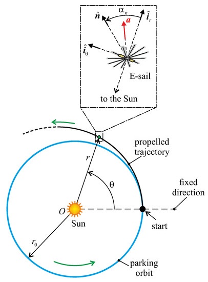
Figure 1.
Polar reference frame and spacecraft states in a two-dimensional mission scenario.
Note that and are the two control variables of our two-dimensional problem.
2.1. Spacecraft Dynamics
The state of the spacecraft in the polar reference frame is defined by the variables , where u (or v) is the radial (or transverse) component of the vehicle inertial velocity. The equations of motion are
where is the Sun’s gravitational parameter. The initial conditions on a circular orbit of radius are
where it is assumed, without loss of generality, that the spacecraft initially orbits the Sun in a counterclockwise direction as is illustrated in Figure 1 (see the green arrows).
The differential Equations (8) and (9) can be rewritten in dimensionless form using the definition of and introducing the dimensionless velocity components and , defined as
and the dimensionless time
where is the initial time. The dimensionless equations of motion are
where the prime symbol denotes a derivative taken with respect to , while the initial conditions (9) become
Since the dimensionless Equations (12)–(15) and the initial conditions (16) do not depend on , the results of the trajectory design discussed in the next subsection will be independent of the radius of the circular parking orbit. As a result, the numerical results obtained from the proposed approach can be easily adapted to a wide range of heliocentric mission scenarios.
2.2. Trajectory Design and Optimization
The aim of this subsection is to design the COFT to obtain a transition from a prograde motion (when the spacecraft flies counterclockwise in the parking orbit sketched in Figure 1) to a retrograde motion (i.e., a motion along the circular parking orbit of Figure 1 with a clockwise direction), using a two-dimensional transfer coplanar with the plane of the parking orbit. We assume that the orbit flip maneuver is completed at time , or , so that, if the final polar angle is left free, the spacecraft states at the (unknown) time are constrained by the equations
or, in dimensionless form
Note that the only difference between Equation (18) and the corresponding initial values of the state variables given by Equation (16) is in the sign of the transverse component of the spacecraft velocity.
The transfer trajectory study is conducted from an optimization perspective, by looking for the COFTs that minimize the flight time for a given value of the dimensionless propulsive acceleration defined in Equation (3). The optimization problem has been solved with an indirect method [31,32], in particular by using the calculus of variations [33] and the Pontryagin’s maximum principle [34] to obtain the optimal control law. The latter coincides with the pair of functions and that maximizes the performance index [35]
The approach used to solve the problem, which is similar to that used by the authors in recent works [36,37], is now summarized for the sake of completeness.
Bearing in mind the equations of motion (12)–(15) and introducing the dimensionless adjoint variables , the Hamiltonian function turns out to be
which is necessary to write the Euler–Lagrange differential equations [38]
in which is the independent variable. The optimal control law is derived from the Pontryagin maximum principle [34] by maximizing, at each instant of time, the Hamiltonian function (20). The result is in agreement with the model proposed in Ref. [28], so that the pitch angle and the switching parameter are expressed as a function of the two dimensionless adjoint variables as
where denotes the signum function, while the auxiliary angle is defined as
The transversality condition [33] provides two additional constraints at the final time
which complete the two-point boundary problem (TPBVP) formed by the four equations of motion (12)–(15), the four Euler-Lagrange differential Equations (21)–(24), and the seven boundary constraints given by Equations (16) and (18). In fact, since in this problem is an output of the optimization process [33], solving the TPBVP requires nine scalar constraints.
For a given value of the dimensionless propulsive acceleration , the TPBVP associated to the optimization process has been solved with an absolute error less than . Note that, according to Equation (22), the adjoint variable is a constant of motion and, taking advantage of Equation (27), we get throughout the flight. The adjoint variable can therefore be removed from the mathematical model, with a slight simplification of the numerical solution.
3. Numerical Simulations and Discussion
The numerical solution of the TPBVP, which has been described at the end of the previous section, gives the COFT as a function of a given value of the dimensionless propulsive acceleration . The TPBVP has been numerically solved using a specific procedure based on the multiple shooting method [39,40,41] and the classical simplex algorithm. Trajectory optimization was conducted considering both a Direct Transfer (DT) scenario and a single Solar Wind Assist (SWA) transfer. The DT and SWA are two types of transfers introduced by the authors [42] by drawing parallels with similar concepts used in an interstellar mission based on a photonic solar sail [43,44,45,46]. In the recent literature, this two concepts have also been used to analyze the optimal transfer to heliostationary points using a very high-performance E-sail [37].
More precisely, in a DT the radial distance increases continuously with time until the spacecraft reaches the aphelion point (subscript a), as shown in Figure 2a. Instead, a trajectory with a (single) SWA contains an initial phase where the spacecraft approaches the Sun to increase its propulsive acceleration magnitude, and then rapidly grows its radial distance to reach the aphelion point [37]; see the scheme of Figure 2b. Note that the mathematical model discussed in the previous section does not include a constraint on the minimum solar distance, that is, a constraint on the perihelion (subscript p) distance, as was considered in the model described in Ref. [37]. Therefore, the (unconstrained) perihelion distance is an output of the optimization process in a transfer with a single SWA.
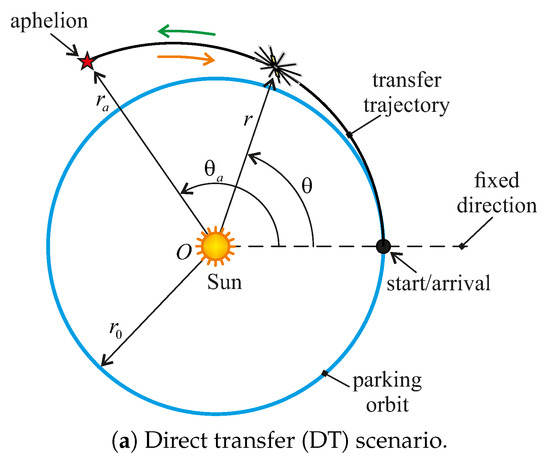
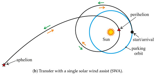
Figure 2.
Conceptual scheme of a COFT of DT type or with a single SWA.
The numerical simulations show that a generic COFT can ideally be divided into two symmetrical parts: (i) a first half part of the transfer trajectory in which the spacecraft reaches, at time , the aphelion point with a zero inertial velocity, that is, with (see the green arrows in Figure 2); (ii) a second half-part in which the spacecraft retraces the trajectory obtained in the first half part backwards until it again reaches the starting point with and (see the orange arrows in Figure 2). In particular, a COFT with a DT has a lenticular shape, while a COFT with a single SWA is characterized by a knot shape that encompasses the Sun. A conceptual sketch of these two possible shapes of a COFT is shown in Figure 2.
The solution of the optimization process indicates that the spacecraft achieves a heliostationary condition (i.e., a zero value of its inertial velocity) at the aphelion of the generic COFT, both in a DT scenario and in a transfer with a single SWA. Such a heliostationary condition is achieved only at a single point along the transfer trajectory, while in the neighboring of the COFT aphelion the spacecraft experiences a quasi-heliostationary condition as the magnitude of its inertial velocity is very small. In the case of solar sail-based mission [3,4,5], such a specific feature of a propelled trajectory has been highlighted by the authors [47] and by Zeng et al. [48,49,50] in a non-Keplerian orbit [51,52] with multiple H-reversal points. In particular, an H-reversal point occurs when the magnitude of the spacecraft angular momentum vector is zero but, usually, it also indicates a point where the angular momentum vector of the osculating orbit reverses its direction.
The concept of H-reversal trajectory was originally proposed by Vulpetti [53,54] in the middle of the 1990s as a possible trajectory of a high (or very-high) performance solar sail [55] in an advanced mission application such as an escape from the Solar System [56], or a fast transfer to the outer regions of our planetary system [57]. The H-reversal trajectory has been also proposed in an asteroid deflection mission, as discussed by Gong et al. [58]. Generally speaking, a multi H-reversal trajectory can be thought of as an extension of Vulpetti’s original idea [53,54]. In fact, in a multi H-reversal trajectory, two (or more) H-reversal points are used to generate a non-Keplerian closed orbit that does not encompass the Sun. This trajectory is then maintained for a long time interval by exploiting the propulsive acceleration given by a propellantless propulsion system such as, for example, a solar sail. This concept is thoroughly illustrated in the recent review by Zeng et al. [26] and in Vulpetti’s book about the so called ‘fast solar sailing’ [59,60,61].
Recalling the results obtained in a solar sail-based scenario [26], an optimal COFT in a DT case can be regarded as half of a particular double H-reversal trajectory, in which the perihelion coincides with the starting position [47]. In contrast, the case where a SWA occurs during an optimal transfer generates a propulsive trajectory that is completely different from the results in the literature. Therefore, the results obtained in the case of a SWA represent a novelty from the point of view of the shapes of optimal trajectories generated by continuous-thrust propulsion systems.
The results of the optimization process, in terms of minimum flight time and characteristics of the optimal COFT, are illustrated in the following two subsections for a DT scenario and a transfer with a single SWA, respectively.
3.1. Case of DT Scenario
For a DT case, Figure 3 shows the ratio of the minimum flight time to the period of the circular parking orbit as a function of . Note that
so that is independent of the radius . Additionally, note that
where is the performance index defined in Equation (19).
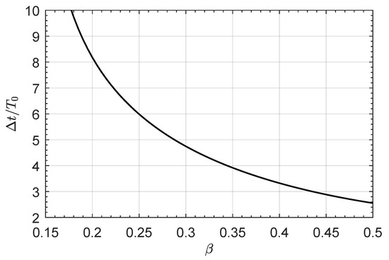
Figure 3.
Case of a DT: ratio of the minimum flight time to the orbital period of the parking orbit as a function of the dimensionless propulsive acceleration .
The curve plotted in Figure 3 can be used to rapidly estimate the transfer performance in an orbit flip mission for an E-sail of given characteristics, starting from a circular orbit of assigned radius. For example, Figure 3 indicates that an E-sail with a propulsive acceleration of travels through the optimal COFT in a time interval of about . In that case, assuming (a scenario compatible with the deployment of the sail just outside the Earth’s sphere of influence when the escape trajectory is parabolic and the eccentricity of the Earth’s orbit is neglected), the period is equal to 1 year, while . The orbital flip is completed in about using an E-sail with a characteristic acceleration of about , corresponding to a medium-high performance propulsion system [62]. As a second example, if the mission is to be completed in less than , Figure 3 states that , that is, it is necessary an E-sail with when .
Since in a DT case the perihelion coincides with the starting point, the position of the COFT aphelion is an output of the optimization process. The simulation results are summarized in Figure 4. The upper part of Figure 4 shows the aphelion distance , while the bottom part shows the angular position (i.e., the polar angle ) of the aphelion point.
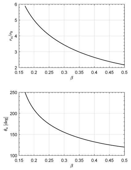
Figure 4.
Case of a DT: radial () and angular () position on the aphelion point as a function of .
For example, assuming again , an optimal COFT obtained with has an aphelion point at a distance of about from the Sun, and the E-sail sweeps a polar angle of about to move from the starting to the aphelion point. This same result is clearly visible in the polar COFT depicted in Figure 5, which also shows the optimal transfer trajectories for different values of .
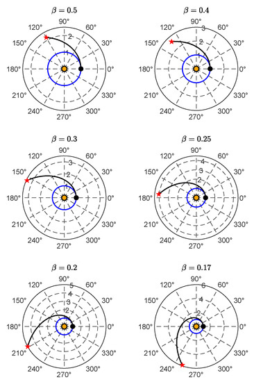
Figure 5.
Polar form of the COFT (black line) for a set of values of the propulsive acceleration in a DT scenario. Black circle → starting point; red star → aphelion; orange circle → Sun; blue line → parking orbit. The radial distance is normalized with the parking orbit radius .
3.2. Case of a Transfer with a Single SWA
Figure 6 shows the minimum flight time for a range of variation of compatible with a medium-performance E-sail. As expected, bearing in mind the results obtained in a Solar System escape scenario [42] or in a more challenging interstellar mission [63], the presence of a SWA allows the E-sail to reduce the flight time compared with the DT case discussed in the previous subsection. Moreover, if a single SWA is included in the trajectory design, the same time of flight as in the DT case can be obtained, but with a reduced value of . For example, a comparison between the curves of Figure 3 and Figure 6 indicates that a flight time of about requires a propulsive acceleration for a DT case, while the same flight time is obtained with in a transfer with a single SWA.
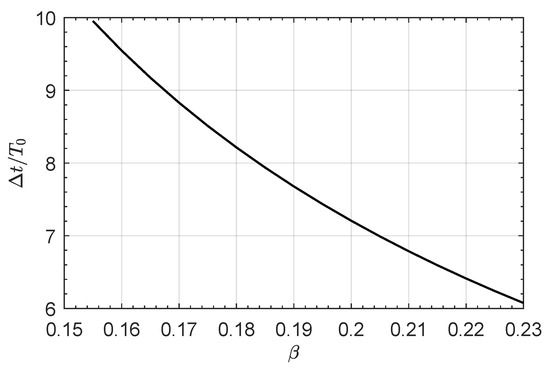
Figure 6.
Case of a transfer with a single SWA: variation of the dimensionless time with .
The presence of a SWA obviously complicates the shape of the transfer trajectory, as confirmed by the schemes in Figure 2 and, more importantly, introduces a perihelion point at a solar distance less than the radius of the circular parking orbit; see Figure 7. Note, however, that Figure 7 does not give the actual value of , but it only reports the ratio as a function of the E-sail propulsive characteristics, so that the actual distance of from the Sun depends on the value of . This is an important consideration, because in an E-sail mission scenario the value of is inferiorly limited by the maximum operating temperature of the conducting tethers. For example, an E-sail structure made of aluminum tethers must operate at a solar distance greater than , while using copper tethers in the sail design reduces the minimum solar distance to about [42]. In the latter case, if the parking orbit radius is , Figure 7 shows that SWA transfers with are unfeasible. If, instead, , Figure 7 states that should be less than about .
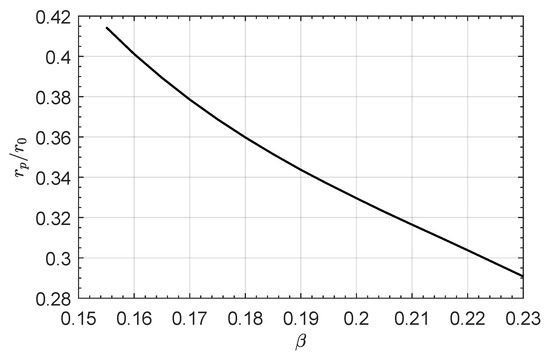
Figure 7.
Case of a transfer with a single SWA: dimensionless radial distance of the perihelion point as a function of the propulsive acceleration .
An illustrative set of COFTs is summarized in Figure 8 for six different values of the dimensionless propulsive acceleration. In particular, the figure shows how the shape of the COFT changes as the value of increases, and in this regard, an interesting behavior concerns the position of the aphelion point, marked by a red star. In fact, Figure 8 shows that decreases as increases, while, in the selected range of , its angular position is essentially in opposition to the starting point. This behavior is confirmed by Figure 9, which shows the coordinates of the aphelion points as a function of .
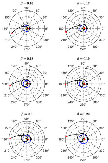
Figure 8.
Polar form of the COFT (black line) for a set of values of the propulsive acceleration in a scenario with a single SWA. Black circle → starting point; red star → aphelion point; orange circle → Sun; blue line → parking orbit. The radial distance is normalized with the parking orbit radius .
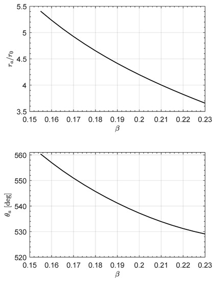
Figure 9.
Case of a transfer with a single SWA: radial () and angular () position of the aphelion point as a function of .
The presence in the optimal COFT of a heliostationary aphelion point with a solar distance on the order of a few multiples of , in both a DT- and SWA-based scenario, suggests a potential (and additional) interesting application of this advanced two-dimensional trajectory concept. In fact, as proposed by the authors a few years ago, a propellantless propulsion system can be used to achieve a linear trajectory (i.e., a Keplerian orbit with a null value of the semilatus rectum) that allows the spacecraft to move along a straight, radial path to regions near the Sun to obtain in situ measurements of the space surrounding our star. Building on that mission concept, in a COFT-based scenario, a “piggy-back” science probe could be released at the aphelion point with a heliocentric velocity equal to zero. Upon release, the main spacecraft (i.e., the vehicle propelled by the E-sail subsystem) would return to the circular parking orbit by retracing the heliocentric path, while the scientific probe would follow the linear trajectory to final destruction in the Sun’s inner regions. This specific mission concept, in the case of a single SWA maneuver, has been schematized in Figure 10, which represents the extended version of the scheme in Figure 2b. In particular, the magenta line in Figure 10 indicates the linear trajectory followed by the science probe after its release (with zero inertial velocity) at the COFT’s aphelion point. Note that the same mission concept can also be applied to a DT case.
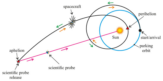
Figure 10.
Conceptual sketch of an extended mission scenario (in presence of a single SWA), in which a scientific probe is released at the aphelion point to cover a linear trajectory. See also Figure 2b.
The mission analysis involving the insertion of a scientific probe into a linear trajectory is one of the possible extensions of the models discussed in this paper, and a couple of other potential extensions are briefly discussed in the conclusion section at the end of this paper. The next subsection, instead, describes the interesting characteristics of the optimal control law in two specific scenarios.
3.3. Mission Applications
The aim of this subsection is to analyze the time variation of the parameters of the osculating orbit and the corresponding optimal control laws in two mission scenarios, each of which were obtained with a different value of . For exemplary purposes we select a value of for the DT case and a different one for the transfer with a single SWA. Note that the general characteristics of the time variation of the two control variables can be shared with other mission scenarios obtained with different values of .
3.3.1. Case of DT with
The first mission example refers to a DT obtained with a medium-high performance E-sail with . According to Figure 3, the minimum flight time is , while the aphelion point has a radial distance and its polar angle is ; see also Figure 4. The polar form of the COFT is shown in one of the plots included in Figure 5, while the time variations of the state variables are reported in Figure 11, where the red star indicates the aphelion point reached during the transfer trajectory.
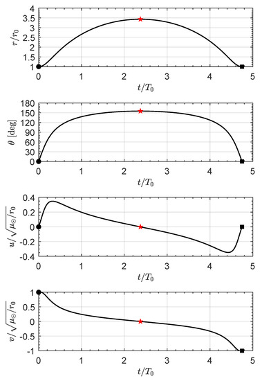
Figure 11.
Time variations of the state variables in a DT scenario with . Black circle → starting point; red star → aphelion point; black square → arrival.
The analysis of the curves reported in Figure 11 confirms that the aphelion point is reached right in the middle of the transfer, and indicates that the variation of is essentially symmetrical over time. This is, of course, a consequence of the spacecraft retracing the same heliocentric trajectory after reaching the aphelion point, as mentioned in the previous section. In the same figure, note how the transverse component v of the spacecraft velocity decreases with time (with a zero value in correspondence of the aphelion, as expected), while the radial component u presents three points in which its value is zero, that is, the {start, aphelion, arrival} points.
Regarding the optimal control law, simulations indicate that the E-sail propulsion system is always on during a DT, so that for . Instead, changes during the transfer and its time variation has the symmetrical form sketched in Figure 12. The interesting aspect that emerges from this figure is that the value of the pitch angle is essentially constant throughout most of the COFT. In fact, from Figure 12 it can be seen that in about of the transfer. This is an interesting behavior, common to the other DTs analyzed in the simulations, because an almost constant value of pitch angle indicates a nearly constant sail attitude in an orbital reference frame. In the context of optimal control laws, a different behavior appears in a transfer with a single SWA, as discussed in the next section.
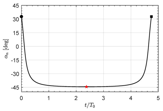
Figure 12.
Time variation of the sail pitch angle in a DT scenario with . Black circle → start; red star → aphelion point; black square → arrival.
3.3.2. Single SWA Transfer with
The presence of a SWA complicates both the transfer trajectory and the optimal control law. For example, assume , which is related to a medium performance E-sail. In the presence of a single SWA, numerical simulations give an optimal transfer with a minimum flight time , a perihelion distance , and an aphelion distance ; see also Figure 6, Figure 7 and Figure 9. The optimal COFT is shown in Figure 13, where the radial distance is in multiples of and the red triangle indicates the perihelion point. Note how the Sun-perihelion distance is well below the radial distance of the starting point (the black circle in the figure), while the aphelion point reaches a high solar distance.
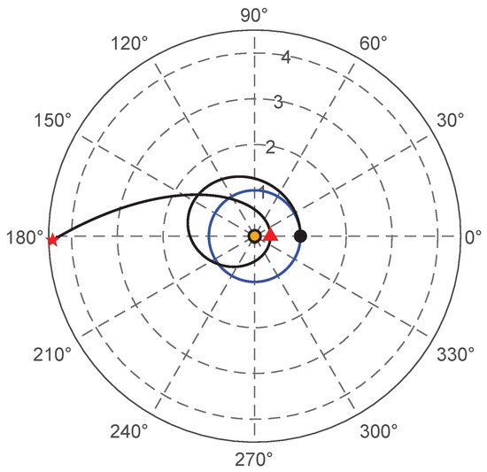
Figure 13.
Polar form of the optimal COFT with a single SWA when . Black circle → starting point; red star → aphelion point; red triangle → perihelion point.
The time variations of the state variables are shown in Figure 14, where the presence of two red triangles indicates that the perihelion point is reached by the spacecraft at two separate instants of time, due to the inherent symmetry of the problem. A comparison between the curves in Figure 14 and those sketched in Figure 11 clearly shows that the general trends of the state variables in a DT and SWA case are profoundly different, even in the presence of a heliostationary condition at the aphelion point. Indeed, note how the two components of the spacecraft velocity are both zero at the midpoint of the COFT.
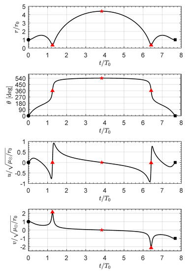
Figure 14.
Time variations of the spacecraft state variables in a SWA transfer with . Black circle → starting point; red star → aphelion point; red triangle → perihelion point; black square → arrival.
Another evident difference between the two transfer concepts (DT and SWA) is in the time variations of the two control parameters . For example, the SWA case with has the optimal control law shown in Figure 15, where the two gray shaded areas indicate the presence of two coasting arcs (when the propulsion system of the electric sail is off), while in the rest of the transfer . Although the two coating arcs have a very small time length, they demonstrate that a condition with can also be optimal from the viewpoint of the flight time minimization [62].
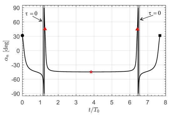
Figure 15.
Time variation of the two control parameters in a SWA transfer with . Black circle → starting point; red star → aphelion point; black square → arrival; red triangle → perihelion point; shaded area →.
4. Final Remarks and Conclusions
In the context of mission scenarios based on the use of E-sails, the present work has proposed a new approach to achieve a complete reversal of the direction of motion along a circular, heliocentric orbit of assigned radius. The orbit reversal maneuver uses a two-dimensional transfer trajectory that is coplanar to the initial parking orbit and uses the continuous thrust provided by a medium-high performance E-sail to suitably change the parameters of the osculating orbit during flight. The concept discussed in this paper stems from observation of the particular shape of a family of H-reversal orbits, originally proposed by Giovanni Vulpetti more than 25 years ago and subsequently studied in detail in more recent literature.
What is interesting is that the analysis of two-dimensional “flip trajectories”, conducted using an optimization approach, revealed the existence of a new class of highly non-Keplerian orbits with the presence of both an H-reversal condition and a close passage to the Sun. Such interesting transfer trajectories allow the two-dimensional orbital flip to be completed in a time interval of a few multiples of the period of the parking orbit, even using a medium-performance E sail. This is an intriguing result, because in the case of a solar sail-based spacecraft, propelled trajectories that include an H-reversal point usually require a high-performance propulsion system, as Vulpetti pointed out in his pioneering work. Therefore, the possibility of achieving this rather exotic orbital transfer with a medium-performance propulsion system indicates a possible new application of the propulsion system invented by Janhunen 20 years ago.
The procedure discussed in this paper can be extended, with relatively low effort, to a solar sail-based mission scenario. In this case, the presence of a flip trajectory with a close pass to the Sun would reduce (when assigning the total flight time) the value of the sail characteristic acceleration required to complete the transfer.
A second possible extension of this work involves comparing the performance of a two-dimensional flip trajectory with that of a cranking maneuver. Indeed, in a mission scenario based on the use of sails (both in the case of the solar sail and the E-sail), when it is necessary to achieve a high variation in the orbital inclination of a heliocentric orbit (as in the case studied in this work), the typical optimal transfer trajectory can ideally be divided into three parts. A first part in which the spacecraft approaches the Sun to increase the maximum modulus of propulsive acceleration, a middle part in which the orbital inclination is changed while keeping the solar distance (usually sufficiently low) essentially constant, and, finally, a third part in which the spacecraft increases the orbital radius to return to the initial solar distance and thus complete the transfer. In this context, an extension of this work could clarify whether the proposed two-dimensional approach provides better performance (in terms of flight time reduction) than the typical three-part procedure for varying orbital inclination. If so, a parametric study of the problem should be conducted, considering both the effect of propulsive performance (i.e., the sail acceleration) and the value of the required change in orbital inclination.
Author Contributions
Conceptualization, A.A.Q.; methodology, A.A.Q.; software, A.A.Q.; writing—original draft preparation, A.A.Q.; writing—review and editing, M.B. and G.M. All authors have read and agreed to the published version of the manuscript.
Funding
This research received no external funding.
Institutional Review Board Statement
Not applicable.
Informed Consent Statement
Not applicable.
Data Availability Statement
Not applicable.
Conflicts of Interest
The authors declare no conflict of interest.
Abbreviations and Symbols
| COFT | circular orbit flip trajectory |
| E-sail | Electric Solar Wind Sail |
| TPBVP | two-point boundary problem |
| Notation | |
| spacecraft characteristic acceleration [mm/s] | |
| reference propulsive acceleration [mm/s] | |
| propulsive acceleration vector [mm/s] | |
| Hamiltonian function | |
| radial unit vector | |
| transverse unit vector | |
| J | performance index [days] |
| sail normal unit vector | |
| O | Sun’s center of mass |
| r | Sun-spacecraft distance [au] |
| Sun-spacecraft unit vector | |
| reference distance [] | |
| t | time [days] |
| polar reference frame | |
| u | radial component of spacecraft velocity [km/s] |
| v | transverse component of spacecraft velocity [km/s] |
| pitch angle [deg] | |
| auxiliary angle [deg] | |
| dimensionless reference propulsive acceleration | |
| spacecraft polar angle [deg] | |
| variable adjoint to | |
| variable adjoint to | |
| variable adjoint to | |
| variable adjoint to | |
| Sun’s gravitational parameter [km/s] | |
| dimensionless control parameter | |
| Subscripts | |
| 0 | initial parking orbit |
| a | aphelion point |
| f | final |
| p | perihelion point |
| Superscripts | |
| · | derivative with respect to time |
| ∼ | dimensionless form |
| derivative with respect to |
References
- Chobotov, V.A. Orbital maneuvers. In Orbital Mechanics; AIAA Education Series; American Institute of Aeronautics and Astronautics Inc.: Reston, VA, USA, 2002; Chapter 5; pp. 89–92. [Google Scholar] [CrossRef]
- Curtis, H.D. Orbital maneuvers. In Orbital Mechanics for Engineering Students; Aerospace Engineering; Butterworth-Heinemann: Cambridge, MA, USA, 2021; Chapter 6; pp. 89–92. [Google Scholar] [CrossRef]
- Fu, B.; Sperber, E.; Eke, F. Solar sail technology—A state of the art review. Prog. Aerosp. Sci. 2016, 86, 1–19. [Google Scholar] [CrossRef]
- Gong, S.; Macdonald, M. Review on solar sail technology. Astrodynamics 2019, 3, 93–125. [Google Scholar] [CrossRef]
- Zhao, P.; Wu, C.; Li, Y. Design and application of solar sailing: A review on key technologies. Chin. J. Aeronaut. 2023, 36, 125–144. [Google Scholar] [CrossRef]
- Bassetto, M.; Niccolai, L.; Quarta, A.A.; Mengali, G. A comprehensive review of Electric Solar Wind Sail concept and its applications. Prog. Aerosp. Sci. 2022, 128, 100768. [Google Scholar] [CrossRef]
- Mengali, G.; Quarta, A.A. Solar Sail Near-Optimal Circular Transfers with Plane Change. J. Guid. Control Dyn. 2009, 32, 456–463. [Google Scholar] [CrossRef]
- Liu, X.; Xu, Y.; Wang, S. Heterodimensional cycle bifurcation with two orbit flips. Nonlinear Dyn. 2015, 79, 2787–2804. [Google Scholar] [CrossRef]
- Valsecchi, G.; Rickman, H.; Morbidelli, A.; Wisniowski, T.; Gabryszewski, R.; Wajer, P. Direct-retrograde orbit flips at planetary close encounters: The role of the Tisserand parameter. Astron. Astrophys. 2022, 667, A91. [Google Scholar] [CrossRef]
- Wang, Y.; Fu, T. An Orbit-flip Mechanism by Eccentric Lidov-Kozai Effect with Stellar Oblateness. Astron. J. 2023, 165, 201. [Google Scholar] [CrossRef]
- Zhang, T.S.; Zhu, D.M. Codimension-4 resonant homoclinic bifurcations with orbit flips and inclination flips. Acta Math. Sin. Engl. Ser. 2015, 31, 1359–1366. [Google Scholar] [CrossRef]
- Janhunen, P. Electric sail for spacecraft propulsion. J. Propuls. Power 2004, 20, 763–764. [Google Scholar] [CrossRef]
- Janhunen, P.; Sandroos, A. Simulation study of solar wind push on a charged wire: Basis of solar wind electric sail propulsion. Ann. Geophys. 2007, 25, 755–767. [Google Scholar] [CrossRef]
- Janhunen, P. The electric sail—A new propulsion method which may enable fast missions to the outer solar system. J. Br. Interplanet. Soc. 2008, 61, 322–325. [Google Scholar]
- Janhunen, P.; Toivanen, P.K.; Polkko, J.; Merikallio, S.; Salminen, P.; Haeggström, E.; Seppänen, H.; Kurppa, R.; Ukkonen, J.; Kiprich, S.; et al. Electric solar wind sail: Toward test missions. Rev. Sci. Instrum. 2010, 81, 111301. [Google Scholar] [CrossRef] [PubMed]
- Rauhala, T.; Seppänen, H.; Ukkonen, J.; Kiprich, S.; Maconi, G.; Janhunen, P.; Hæggström, E. Automatic 4-wire Heytether production for the electric solar wind sail. In Proceedings of the International Microelectronics Assembly and Packing Society Topical Workshop and Tabletop Exhibition on Wire Bonding, San Jose, CA, USA, 22–23 January 2013. [Google Scholar]
- Seppänen, H.; Rauhala, T.; Kiprich, S.; Ukkonen, J.; Simonsson, M.; Kurppa, R.; Janhunen, P.; Hæggström, E. One kilometer (1 km) electric solar wind sail tether produced automatically. Rev. Sci. Instruments 2013, 84, 095102. [Google Scholar] [CrossRef]
- Janhunen, P.; Toivanen, P.K. TI tether ring for solving secular spinrate change problem of electric sail. arXiv 2017, arXiv:1603.05563. [Google Scholar]
- Janhunen, P.; Merikallio, S.; Paton, M. EMMI—Electric solar wind sail facilitated Manned Mars Initiative. Acta Astronaut. 2015, 113, 22–28. [Google Scholar] [CrossRef]
- Sanchez-Torres, A. Propulsive force in an electric solar sail. Contrib. Plasma Phys. 2014, 54, 314–319. [Google Scholar] [CrossRef]
- Toivanen, P.K.; Janhunen, P. Spin plane control and thrust vectoring of electric solar wind sail. J. Propuls. Power 2013, 29, 178–185. [Google Scholar] [CrossRef]
- Toivanen, P.K.; Janhunen, P. Thrust vectoring of an electric solar wind sail with a realistic sail shape. Acta Astronaut. 2017, 131, 145–151. [Google Scholar] [CrossRef]
- Bassetto, M.; Mengali, G.; Quarta, A.A. Thrust and torque vector characteristics of axially-symmetric E-sail. Acta Astronaut. 2018, 146, 134–143. [Google Scholar] [CrossRef]
- Janhunen, P. Photonic spin control for solar wind electric sail. Acta Astronaut. 2013, 83, 85–90. [Google Scholar] [CrossRef]
- Wang, R.; Wei, C.; Wu, Y.; Zhao, Y. The study of spin control of flexible electric sail using the absolute nodal coordinate formulation. In Proceedings of the IEEE International Conference on Cybernetics and Intelligent Systems, CIS 2017 and IEEE Conference on Robotics, Automation and Mechatronics, RAM, Ningbo, China, 19–21 November 2017; pp. 785–790. [Google Scholar] [CrossRef]
- Zeng, X.; Vulpetti, G.; Circi, C. Solar sail H-reversal trajectory: A review of its advances and applications. Astrodynamics 2019, 3, 1–15. [Google Scholar] [CrossRef]
- Quarta, A.A.; Abu Salem, K.; Palaia, G. Solar sail transfer trajectory design for comet 29P/Schwassmann-Wachmann 1 rendezvous. Appl. Sci. 2023, 13, 9590. [Google Scholar] [CrossRef]
- Huo, M.Y.; Mengali, G.; Quarta, A.A. Electric sail thrust model from a geometrical perspective. J. Guid. Control Dyn. 2018, 41, 735–741. [Google Scholar] [CrossRef]
- Janhunen, P. Increased electric sail thrust through removal of trapped shielding electrons by orbit chaotisation due to spacecraft body. Ann. Geophys. 2009, 27, 3089–3100. [Google Scholar] [CrossRef]
- Quarta, A.A.; Mengali, G.; Bassetto, M.; Niccolai, L. Optimal circle-to-ellipse orbit transfer for Sun-facing E-sail. Aerospace 2022, 9, 671. [Google Scholar] [CrossRef]
- Betts, J.T. Survey of Numerical Methods for Trajectory Optimization. J. Guid. Control Dyn. 1998, 21, 193–207. [Google Scholar] [CrossRef]
- von Stryk, O.; Bulirsch, R. Direct and indirect methods for trajectory optimization. Ann. Oper. Res. 1992, 37, 357–373. [Google Scholar] [CrossRef]
- Bryson, A.E.; Ho, Y.C. Optimization problems for dynamic systems. In Applied Optimal Control; Hemisphere Publishing Corporation: New York, NY, USA, 1975; Chapter 2; pp. 71–89. ISBN 0-891-16228-3. [Google Scholar]
- Ross, I.M. Pontryagin’s principle. In A Primer on Pontryagin’s Principle in Optimal Control; Collegiate Publishers: San Francisco, CA, USA, 2015; Chapter 2; pp. 127–129. [Google Scholar]
- Stengel, R.F. Optimal Control and Estimation; Dover Books on Mathematics; Dover Publications, Inc.: New York, NY, USA, 1994; pp. 222–254. [Google Scholar]
- Mengali, G.; Quarta, A.A. E-Sail Option for Plunging a Spacecraft into the Sun’s Atmosphere. Aerospace 2023, 10, 340. [Google Scholar] [CrossRef]
- Quarta, A.A.; Mengali, G. E-sail optimal trajectories to heliostationary points. Aerospace 2023, 10, 194. [Google Scholar] [CrossRef]
- Lawden, D.F. Optimal Trajectories for Space Navigation; Butterworths & Co.: London, UK, 1963; pp. 54–60. [Google Scholar]
- Bakhtiari, M.; Abbasali, E.; Sabzy, S.; Kosari, A. Natural coupled orbit—Attitude periodic motions in the perturbed-CRTBP including radiated primary and oblate secondary. Astrodynamics 2022, 7, 229–249. [Google Scholar] [CrossRef]
- Guzzetti, D.; Howell, K.C. Coupled Orbit-Attitude Dynamics in the Three-Body Problem: A Family of Orbit-Attitude Periodic Solutions. In Proceedings of the AIAA/AAS Astrodynamics Specialist Conference, San Diego, CA, USA, 4–7 August 2014. [Google Scholar] [CrossRef]
- Abbasali, E.; Kosari, A.; Bakhtiari, M. Effects of oblateness of the primaries on natural periodic orbit-attitude behaviour of satellites in three body problem. Adv. Space Res. 2021, 68, 4379–4397. [Google Scholar] [CrossRef]
- Quarta, A.A.; Mengali, G. Electric sail mission analysis for outer solar system exploration. J. Guid. Control Dyn. 2010, 33, 740–755. [Google Scholar] [CrossRef]
- Lyngvi, A.; Falkner, P.; Kemble, S.; Leipold, M.; Peacock, A. The Interstellar Heliopause Probe. Acta Astronaut. 2005, 57, 104–111. [Google Scholar] [CrossRef]
- Leipold, M.; Wagner, O. ‘Solar Photonic Assist’ Trajectory Design for Solar Sail Missions to the Outer Solar System and Beyond. In Proceedings of the AAS/GSFC 13th International Symposium on Space Flight Dynamics, Greenbelt, MD, USA, 11–15 May 1998. [Google Scholar]
- Lappas, V.; Leipold, M.; Lyngvi, A.; Falkner, P.; Fichtner, H.; Kraft, S. Interstellar Heliopause Probe: System Design of a Solar Sail Mission to 200 AU. In Proceedings of the AIAA Guidance, Navigation, and Control Conference and Exhibit, San Francisco, CA, USA, 15–18 August 2005. [Google Scholar] [CrossRef]
- Dachwald, B. Optimization of Interplanetary Solar Sailcraft Trajectories Using Evolutionary Neurocontrol. J. Guid. Control Dyn. 2004, 27, 66–72. [Google Scholar] [CrossRef]
- Mengali, G.; Quarta, A.A.; Romagnoli, D.; Circi, C. H2-reversal trajectory: A new mission application for high-performance solar sails. Adv. Space Res. 2011, 48, 1763–1777. [Google Scholar] [CrossRef]
- Zeng, X.; Baoyin, H.; Li, J.F.; Gong, S.P. New applications of the H-reversal trajectory using solar sails. Res. Astron. Astrophys. 2011, 11, 863–878. [Google Scholar] [CrossRef]
- Zeng, X.; Baoyin, H.; Li, J.; Gong, S. Feasibility analysis of the angular momentum reversal trajectory via hodograph method for high performance solar sails. Sci. China Technol. Sci. 2011, 54, 2951–2957. [Google Scholar] [CrossRef]
- Zeng, X.; Alfriend, K.T.; Vadali, S.R. Three-dimensional time Optimal Multi-reversal Orbit by Using Solar Sailing. J. Astronaut. Sci. 2013, 60, 378–395. [Google Scholar] [CrossRef]
- McInnes, C.R. Solar sail mission applications for non-Keplerian orbits. Acta Astronaut. 1999, 45, 567–575. [Google Scholar] [CrossRef]
- McKay, R.J.; Macdonald, M.; Biggs, J.; McInnes, C. Survey of Highly Non-Keplerian Orbits with Low-Thrust Propulsion. J. Guid. Control Dyn. 2011, 34, 645–666. [Google Scholar] [CrossRef]
- Vulpetti, G. General 3D H-reversal trajectories for high-speed sailcraft. Acta Astronaut. 1999, 44, 67–73. [Google Scholar] [CrossRef]
- Vulpetti, G. Sailcraft at high speed by orbital angular momentum reversal. Acta Astronaut. 1997, 40, 733–758. [Google Scholar] [CrossRef]
- Scaglione, S.; Vulpetti, G. Aurora project: Removal of plastic substrate to obtain an all-metal solar sail. Acta Astronaut. 1999, 44, 147–150. [Google Scholar] [CrossRef]
- Vulpetti, G. Reaching extra-solar-system targets via large post-perihelion lightness-jumping sailcraft. Acta Astronaut. 2011, 68, 636–643. [Google Scholar] [CrossRef]
- Vulpetti, G. The sailcraft splitting concept. J. Br. Interplanet. Soc. 2006, 59, 48–53. [Google Scholar]
- Gong, S.P.; Li, J.F.; Zeng, X.Y. Utilization of an H-reversal trajectory of a solar sail for asteroid deflection. Res. Astron. Astrophys. 2011, 11, 1123–1133. [Google Scholar] [CrossRef]
- Vulpetti, G. Sailcraft Trajectories. In Solar Sails: A Novel Approach to Interplanetary Travel; Springer-Praxis Books in Space Exploration; Springer: New York, NY, USA, 2009; Chapter 17; pp. 216–224. [Google Scholar] [CrossRef]
- Vulpetti, G. Fast Solar Sailing: Astrodynamics of Special Sailcraft Trajectories; Space Technology Library; Springer: Dordrecht, The Netherlands, 2013. [Google Scholar] [CrossRef]
- Davoyan, A. Extreme solar sailing for fast transit exploration of solar system and interstellar medium. In Proceedings of the ASCEND 2021, Online, 15–17 November 2021. [Google Scholar] [CrossRef]
- Mengali, G.; Quarta, A.A.; Janhunen, P. Electric sail performance analysis. J. Spacecr. Rockets 2008, 45, 122–129. [Google Scholar] [CrossRef]
- Huo, M.Y.; Mengali, G.; Quarta, A.A. Mission design for an interstellar probe with E-sail propulsion system. J. Br. Interplanet. Soc. 2015, 68, 128–134. [Google Scholar]
Disclaimer/Publisher’s Note: The statements, opinions and data contained in all publications are solely those of the individual author(s) and contributor(s) and not of MDPI and/or the editor(s). MDPI and/or the editor(s) disclaim responsibility for any injury to people or property resulting from any ideas, methods, instructions or products referred to in the content. |
© 2023 by the authors. Licensee MDPI, Basel, Switzerland. This article is an open access article distributed under the terms and conditions of the Creative Commons Attribution (CC BY) license (https://creativecommons.org/licenses/by/4.0/).