Noise Reduction Based on a CEEMD-WPT Crack Acoustic Emission Dataset

Abstract

In order to solve the noise reduction problem of acoustic emission signals with cracks, a method combining Complementary Ensemble Empirical Mode Decomposition (CEEMD) and wavelet packet (WPT) is proposed and named CEEMD-WPT. Firstly, the single Empirical Mode Decomposition (EMD) used in the traditional CEEMD is improved into the WPT-EMD with a more stable noise reduction effect. Secondly, after decomposition, the threshold value of the correlation coefficient is determined for the Intrinsic Mode Function (IMF), and the low correlation component is further processed by WPT. In addition, in order to solve the problem that it is difficult to quantify the real signal noise reduction effect, a new quantization index “principal interval coefficient (PIC)” is designed in this paper, and its reliability is verified through simulation experiments. Finally, noise reduction experiments are carried out on the real crack acoustic emission dataset consisting of tensile, shear, and mixed signals. The results show that CEEMD-WPT has the highest number of signals with a principal interval coefficient of 0–0.2, which has a better noise reduction effect compared with traditional CEEMD and Complementary Ensemble Empirical Mode Decomposition with Adaptive Noise (CEEMDAN). Moreover, the statistical variance of CEEMD-WPT is evidently one order of magnitude smaller than that of CEEMD, so it has stronger stability.

1. Introduction

As a kind of damage, cracks seriously affect the performance of a structure, exist in all walks of life, and can be a hidden danger for a subsequent accident. Acoustic emission (AE) refers to the elastic wave released through the structural medium when microcracks occur [1,2]. AE is a structural health monitoring (SHM) technology [3], which has the advantages of online monitoring, high sensitivity, and early and rapid defect detection [4,5,6,7]. It has been widely used in machinery, geology, materials, and other fields, and has obtained a lot of achievements [8].

The shear fracture of material structures usually begins with microcracks produced by stretching [9], so it is of great significance to detect and classify early cracks. Eline et al. [10] proposed a method combining acoustic emission sensors and vibration monitoring to study the corrosion cracking of reinforced concrete. They proved that acoustic emission technology can accurately predict concrete cracking, whereas vibration monitoring is not sensitive to early defects but can locate damage in a wider range, and the two methods can complement each other. Tayfur et al. [11] distinguished the AE signals of cracking and the fiber desticking of steel-fiber concrete through principal component analysis, and found that the “rise time and count” and “duration and amplitude” of the two signals had the most obvious difference. Kononenko, Y.D. et al. [12] studied acoustic emission signals in the Laser Powder Bed Fusion (L-PBF) process and used the machine learning model to classify crack events and noise, but the effect of this method in the low signal-to-noise ratio environment has not been verified. Lequn et al. [13] used the traditional machine learning model and convolutional neural network (CNN) model to study the classification effect of defects, such as Laser-Assisted Direct Energy Deposition (LDED) cracks, under different characteristic parameters, and the results showed that the Mel Frequency Cepstral Coefficients (MFCC)-CNN proposed in the paper had the best effect.

The application of acoustic emission technology is also difficult, and the recording of acoustic emission signals may be affected by the environment and contact area to produce noise [14]. For this reason, scholars have proposed a variety of noise reduction methods.

The most commonly used noise reduction algorithms are wavelet and Empirical Mode Decomposition (EMD) and their derivatives, such as WPT, Ensemble Empirical Mode Decomposition (EEMD), CEEMD, CEEMDAN, and Variational Mode Decomposition (VMD). Among them, Liu et al. [15] proposed a new threshold function and applied it in wavelet threshold noise reduction. The effectiveness of the method was proved in turbine tests, and the selection of the threshold had a direct impact on the noise reduction effect. The wavelet algorithm has been widely used in acoustic emission signal noise reduction and has achieved good results, but it also has some inherent defects, such as the effect of the wavelet based on noise reduction. Hassan et al. [16] pointed out that the denoising performance is affected by factors such as wavelet basis function, decomposition level, threshold method, and threshold selection criteria, whereas traditional parameter selection methods rely on statistics and experience. This team proposed a threshold denoising method based on a hybrid particle swarm optimization algorithm and compared five common denoising methods. The results show that this method is more effective. He et al. [17] found that the wavelet noise reduction method using a single basis function had poor effects in the face of low signal-to-noise ratio signals with the same frequency interference. A noise reduction method based on EMD and wavelet packets was proposed to solve this problem, and its reliability is proved through welding crack experiments. Hu [18] and others, in order to improve the denoising effect, combined CEEMD and an improved wavelet threshold denoising method for adaptive noise reduction; the acoustic emission signal was first decomposed via CEEMD and then an improved threshold denoising method was used to decompose the IMF component for noise reduction processing, and they verified the effectiveness of the proposed method in mechanical seal acoustic emission experiments. Sun et al. [19] proposed a prediction model combining CEEMDAN, Long Short-Term Memory (LSTM), and Improved Particle Swarm Optimization (IPSO) in the study of the vibration of hydropower units. Zhang et al. [20] combined VMD and Akaike information criteria (AIC); a germplasm denoising method for microseismic signal denoising was designed, and its performance in MS signal processing at Shuangjiang Water Station was demonstrated. Jing et al. [21] designed a noise reduction method combining VMD and fuzzy entropy to remove non-linear noise in coal mine monitoring systems. Chen et al. [22] combined CEEMD, Auto-Regressive Integrated Moving Average (ARIMA), and SVM to design a wind speed prediction model. The model predicted and summarized the CEEMD component and the reconstructed SVM decomposition component of the signal, respectively, with the predicted wind speed. The CEEMDAN–wavelet packet noise reduction algorithm proposed by Yang et al. [23] had the same feature as the most current improvements based on the EMD algorithm [24,25,26], which provided the “selective processing of decomposed IMF components” without making innovations in the decomposition process.

Although the traditional CEEMD noise reduction algorithm has good performance in a large number of acoustic emission studies, it is affected by the addition of random white noise; the noise reduction effect will fluctuate and even have poor noise reduction results. In this paper, an improved CEEMD-WPT noise reduction algorithm is proposed to solve the above problems. The experimental results show that, compared with the traditional CEEMD and CEEMDAN noise reduction algorithms, it has the best noise reduction effect and greatly improves the stability of noise reduction. The algorithm is expected to provide a cleaner signal for the subsequent recognition process, and is of great significance for improving the performance of the SHM system. In addition, this paper designed a “principal interval coefficient” to solve the problem of there being no reliable quantitative evaluation index for the actual signal noise reduction effect at present, and proved its reliability through experimentation. The proposed index makes it easier for future researchers to quantify noise.

2. Basic Theory

2.1. CEEMD Noise Reduction

In order to solve the problem of mode aliasing in EMD, scholars proposed EEMD, which first added multiple groups of white noise to the original signal, then repeated EMD, and finally averaged the overall IMF component. However, it did not completely solve the problem of mode aliasing, but led to increased computation and noise residue. Different from the EEMD method, CEEMD adopts the method of adding white noise in pairs to solve the problem of noise residue, and its process is as follows:

(1)

First, white noise is added in pairs to the original signal.

$$x_i(t)=\left\{\begin{array}{c}x(t)+{\epsilon }^i(t)\\ x(t)-{\epsilon }^i(t)\end{array}\right.,i=1,2, . . . ,n$$

(1)

In the above formula, x(t) is the original signal; εⁱ(t) is white noise; and x_i(t) is the signal pair after adding noise.

(2)

The x_i(t) signal pair is decomposed using EMD.

$$IMF\mathrm{s}=EMD(x_i(t))$$

(2)

(3)

The average value of the 2n group IMFs component is calculated, which is the result of CEEMD.

$$\overline{IMF}=\frac{1}{2n}{\displaystyle \sum _{i=1}^{2n}IM{F}_{ij}(t)}$$

(3)

In the above formula, IMF_ij(t) is the JTH component of the ith signal decomposition.

2.2. WPT Noise Reduction

WPT is improved from wavelet transform, which improves the problem of the insufficient high-frequency resolution of wavelet decomposition by decomposing the high-frequency part. Its process is as follows [27]:

(1)

A set of orthogonal wavelet bases is used to decompose the input signal into two parts: high frequency and low frequency, where the scale function α(t) and the wavelet function β(t) are calculated as follows:

$$\alpha (t)=\sqrt{2}{\displaystyle \sum _{n}l(n)}\alpha (2t-n)$$

(4)

$$\beta (t)=\sqrt{2}{\displaystyle \sum _{n}h(n)}\beta (2t-n)$$

(5)

In the above equation, n is the translation coefficient and l(n) and h(n) are low-pass and high-pass filters, respectively.

(2)

The signal is decomposed by a wavelet packet.

$$d_{i+1}^{2k}={\displaystyle \sum _{n}l(n-2t)}{d}_i^k(n)$$

(6)

$$d_{i+1}^{2k+1}={\displaystyle \sum _{n}h(n-2t)}{d}_i^k(n)$$

(7)

In the above equation, d_i^k(n) is the NTH coefficient of the k node of the i layer of wavelet packet decomposition.

(3)

The threshold method is used to process the wavelet packet coefficient and reconstruct the wavelet coefficient to obtain the signal after noise reduction.

$$d_i^k(n)=2\left[\begin{array}{l}{\displaystyle \sum _{t}l(n-2t)}{d}_{i+1}^{2k+1}(n)+\\ {\displaystyle \sum _{t}h(n-2t)}{d}_{i+1}^{2k}(n)\end{array}\right]$$

(8)

3. Improved CEEMD-WPT Noise Reduction Algorithm

3.1. Improved CEEMD-WPT Decomposition Method

CEEMD smoothed the abrupt points in the signal by adding white noise to solve the mode aliasing problem caused by the discontinuity points, which is still essentially a single EMD.

According to the study of Yu [28] et al., the Wavelat decomposition of signals first has a more obvious noise reduction effect on EMD and also improves stability.

In order to increase the processing effect of high-frequency signals, Wavelat-EMD is improved to WPT-EMD, which replaces the single EMD used in traditional CEEMD. The adopted WPT noise reduction was set according to the parameters in Ref. [28]. The wavelet basis was all “db10”, the decomposition layer number was 3, the soft threshold method was used, and the threshold was calculated using the rigrsure principle.

3.2. Improved CEEMD-WPT Reconstruction Method

After CEEMD is improved, the crack acoustic emission signal is decomposed into a series of IMF components and residue. According to the decomposition principle, the high-frequency part of the signal (containing a large number of random noise) is decomposed into the IMF component at the front, while the low-frequency part (effective signal) is in the rear component, and the component can be distinguished by the mutual relation number.

The correlation number is an indicator used to measure the degree of similarity between two signals.

$$C_i=\frac{cov(IM{F}_i,x(t\left)\right)}{\sqrt{Var(IM{F}_i)Var(x(t))}}$$

(9)

In Equation (9), IMF_i is the i IMF component and x(t) is the original signal.

It is feasible to use the correlation number as an indicator to distinguish the effective signal content in the IMF component, i.e., the effective signal has a greater correlation with the original signal, and the correlation number is larger. In this case, the IMF with a greater correlation number with the original signal is called the strongly correlated component. On the contrary, it has been shown that IMF components contain more noise components, which are called weak correlation components. In addition, the mean of the correlation number between all IMF components and the original signal is calculated as the index to judge the strong and weak correlation components. In addition, in order to prevent the IMF component of some signals from being decomposed too much and thus dragging down the average, we set the mean lower limit here at 0.3, and if it is below this lower limit, it is calculated as 0.3.

$$\overline{C}=\frac{1}{n}{\displaystyle \sum _{i=1}^n{C}_i}$$

(10)

$$T=\begin{array}{cc}\left\{\begin{array}{c}\overline{C}\\ 0.3\end{array}\right.& \begin{array}{c}\overline{C}>0.3\\ \overline{C}\le 0.3\end{array}\end{array}$$

(11)

Because the weakly correlated portion contains a small amount of effective signal and a large amount of noise, it needs to be re-denoised via WPT. However, the strong correlation component has a high content of effective signals, and reprocessing the signal will have the risk of the loss of effective signals. Therefore, the strong correlation component and the weak correlation component after WPT processing are directly reconstructed.

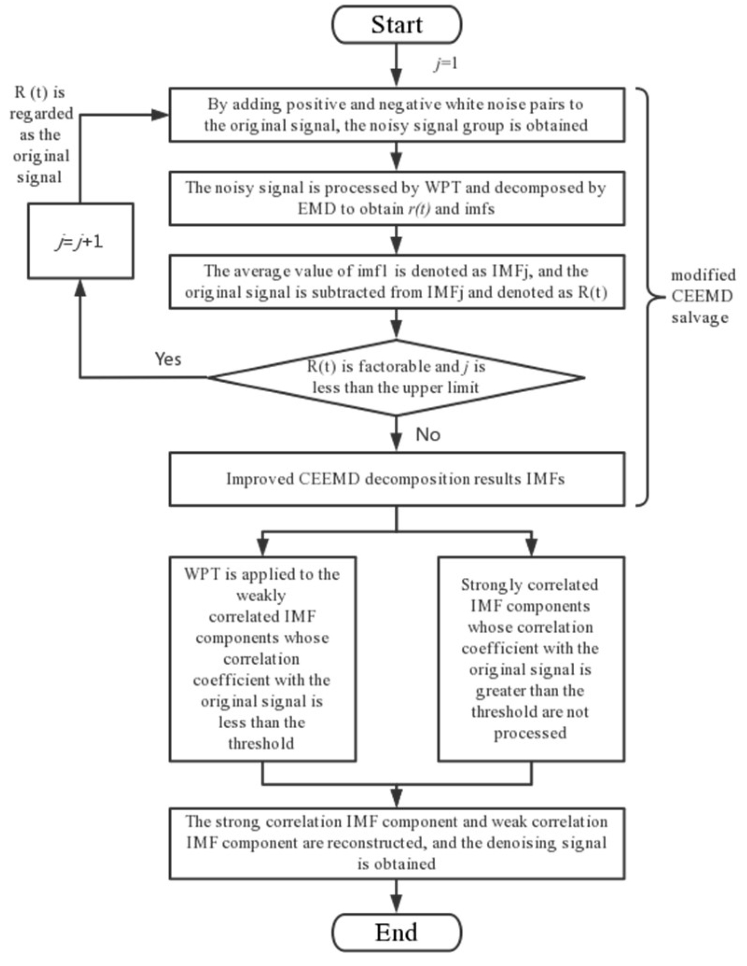
3.3. Improve the Algorithm Steps of CEEMD-WPT

The detailed steps of this method are shown in Figure 1.

(1)

Add n white noise to the collected signal x(t) to obtain a noisy signal group.

(2)

Process the noisy signal group with WPT first, and then with EMD to obtain the n imfs components and residual r(t).

(3)

Calculate the average value of imf1 as IMFj, and subtract IMFj from the original signal as R(t).

(4)

If R(t) can be decomposed or the number of decompositions is lower than the upper limit, then cycle steps (2–4).

(5)

Eliminate the residual r(t), and obtain the IMFs of improved CEEMD.

(6)

Calculate the correlation coefficient between each component in IMFs and the original signal, and distinguish the strong and weak correlation components according to the threshold value.

(7)

Conduct WPT noise reduction for weakly correlated components to remove noise components.

(8)

Reconstruct the weakly correlated component and the strongly correlated component with EMD, and finally obtain the signal x’(t) after noise reduction.

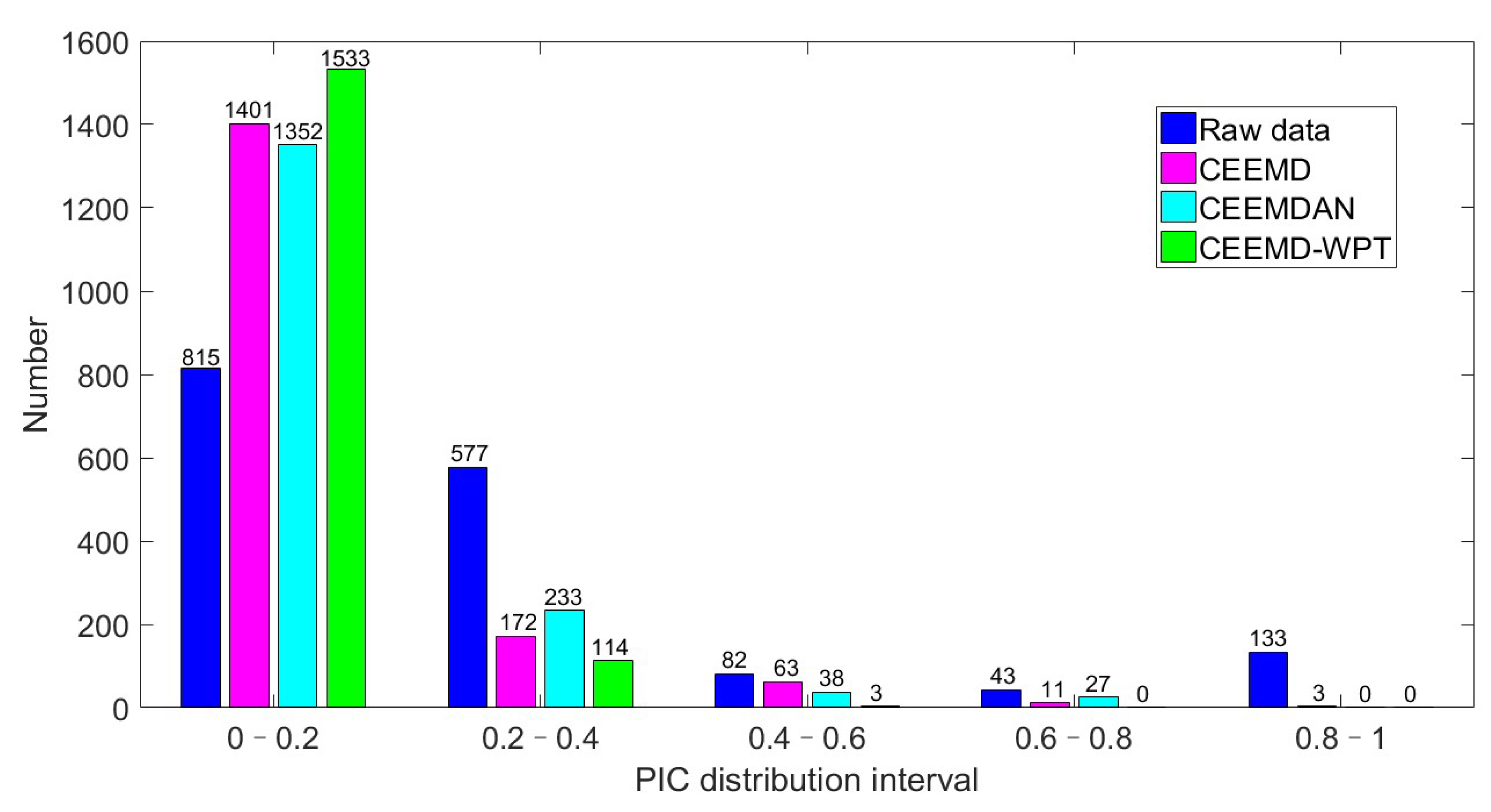
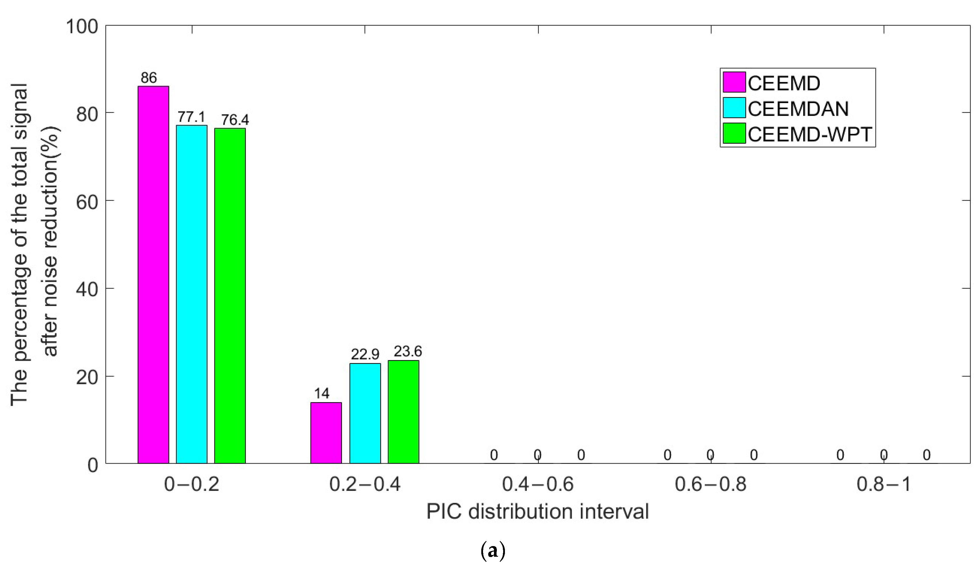
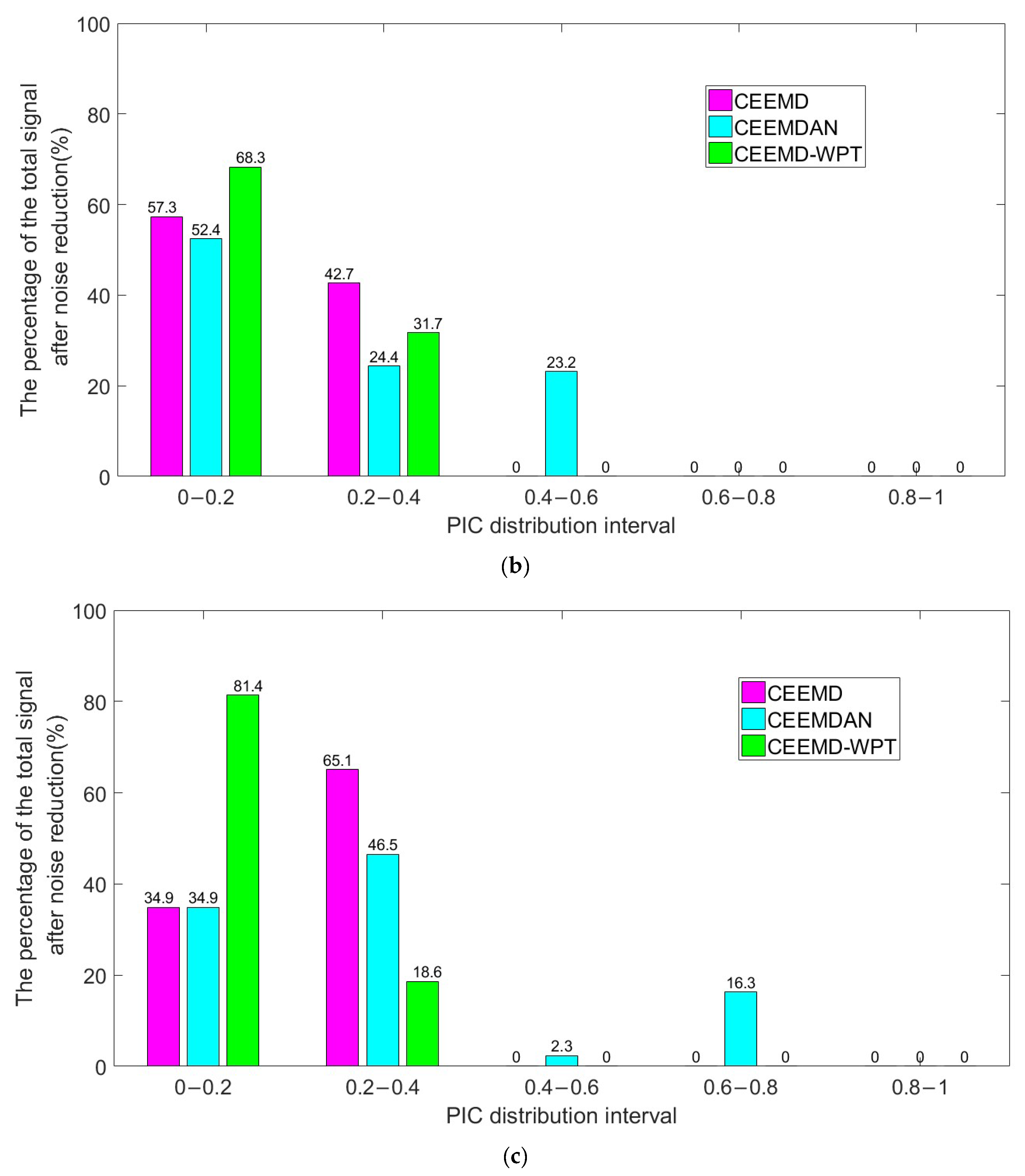
3.4. Principal Interval Coefficient

At present, the main quantitative indicators of the noise reduction effect include the signal-to-noise ratio (SNR), root mean square error (RMSE), and noise reduction error ratio (dnSNR), etc. Their calculation methods are shown in Equations (12)–(14). Because pure signal or noisy signal is unknown in the real signal, the SNR and RMS error cannot measure the noise reduction effect of the real signal. The noise reduction error ratio only focuses on the ratio of signal power before and after noise reduction, so it can be used to quantify the noise reduction effect of the real signal. However, it does not pay attention to the specific components of the eliminated signal, even if the eliminated signal is effective; it can produce a better value, so the quantization reliability of the noise reduction effect is poor.

$$SNR=10\lg \left[\frac{{\displaystyle \sum _{t=1}^{n}Y{\left(t\right)}^2}}{{\displaystyle \sum _{t=1}^n{\left(Y\left(t\right)-\mathrm{y}(t)\right)}^2}}\right]$$

(12)

$$RMSE=\sqrt{\frac{1}{n}{\displaystyle \sum _{t=1}^n{(Y(t)-\mathrm{y}(t))}^2}}$$

(13)

$$\mathrm{dn}SNR=10\lg \left[\frac{{\displaystyle \sum _{t=1}^{n}x{\left(t\right)}^2}}{{\displaystyle \sum _{t=1}^{n}y{\left(t\right)}^2}}\right]$$

(14)

In the above equation, n is the signal length, Y(t) is the pure signal, x(t) is the signal before noise reduction, and y(t) is the signal after noise reduction.

In order to solve the problem of the noise reduction effect of the real signal not being quantified reliably, this paper designs a new quantization parameter “principal interval coefficient (PIC)” according to the fact that the noise is mostly concentrated in the high-frequency band. The practical significance of the principal interval coefficient is the ratio of the frequency interval occupied by the top 90% amplitude to the total frequency interval on the spectrum diagram. The specific calculation method is shown in Equation (15).

$$PIC=\frac{{\left(0.9{\displaystyle \sum _{i=1}^n{A}_i}\right)}^{*}}{H}$$

(15)

In the above equation, PIC is the main interval coefficient, A_i is the amplitude corresponding to frequency i in the spectrum diagram, n is the maximum frequency, H is the total frequency interval, and the (x)* function is the frequency interval corresponding to x.

The quantization principle of the PIC on the signal noise reduction effect is that the effective signal is mainly concentrated in the low-frequency region. When the effective signal content in the signal is higher, the frequency is more concentrated in the low frequency, and the frequency interval occupied by the top 90% amplitude will also decrease, ultimately reducing the PIC index. On the contrary, when there is a lot of noise in the signal, the PICindex will rise. Therefore, the noise reduction effect of the algorithm and the amount of noise contained in the signal can be judged according to the PIC index of the signal before and after noise reduction.

Since the parameters needed to calculate the PIC can be obtained directly from the signal, it can be used to quantify the noise reduction effect of the real signal, which is more practical than the SNR and RMSE. Compared with the dnSNR, the PIC is calculated based on the distribution characteristics of the effective signal and noise, so the quantization results are more reliable. The reliability of the quantization effects of the dnSNR and the PIC is verified in Section 4.

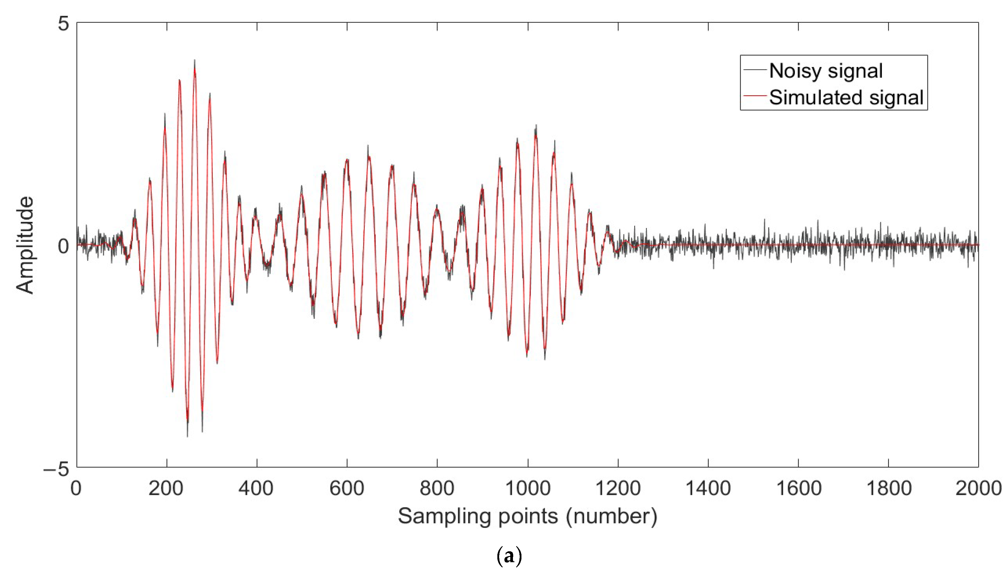
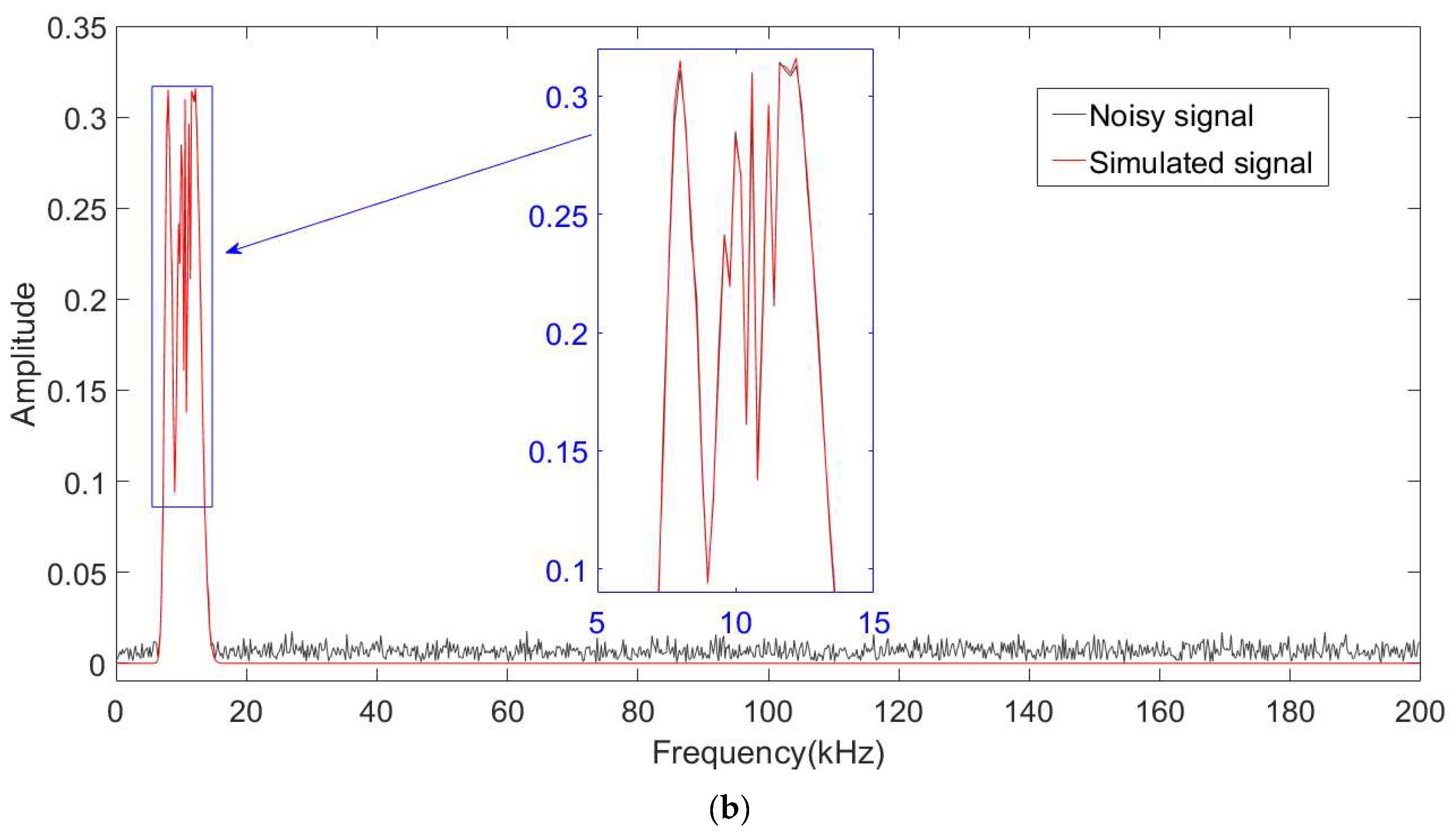
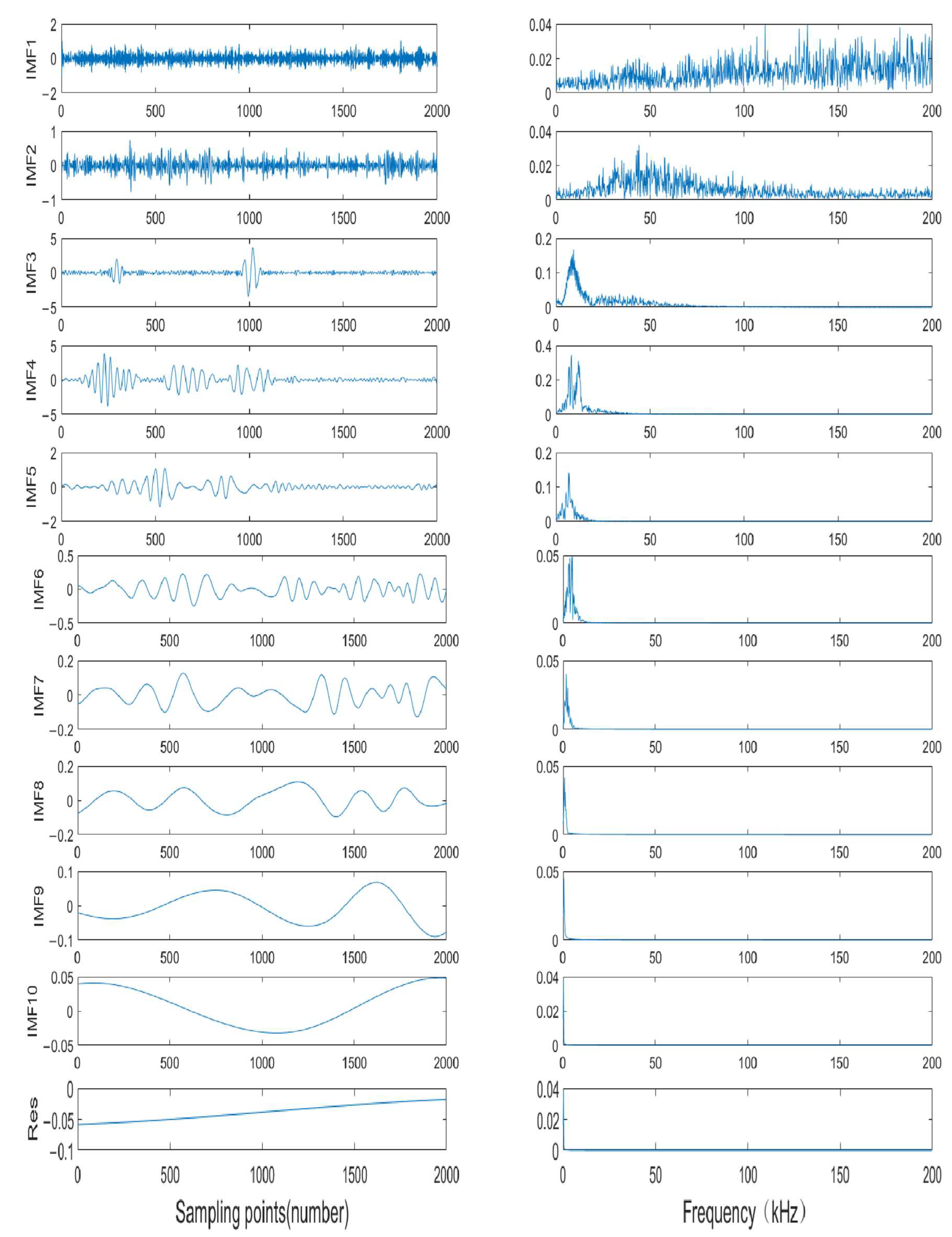
4. Simulation Analysis

In order to verify the noise reduction effect of CEEMD-WPT and the PIC quantization effect proposed in this paper, the AE signal digital model proposed by Mitrakovic et al. [29] is introduced here for the simulation experiments. The model expression is shown in Equation (16):

$$f(t)={\displaystyle \sum _{i=1}^n{A}_i{e}^{\left[-Q_i{(t-t_i)}^2\right]}\sin [2\pi f_i(t-t_i)]}$$

(16)

In the above equation, A_i is the amplitude of the signal, Q_i is the attenuation factor of the signal, t_i is the delay time of the signal, f_i is the frequency of the signal, and n is the number of superposition signals.

The simulation parameters adopted are listed in

Table 1. Analog signal parameters.

Parameter	Ai	Qi	ti (ms)	fi (kHz)
i = 1	4	500	4 × 10−1.5	60
i = 2	2	120	4 × 10−1.1	40
i = 3	2.5	300	4 × 10−0.9	50

, and the waveform and spectrum diagram are shown in the red line in Figure 2. In order to simulate the noise of the environment, white noise with a signal-to-noise ratio of 5 db is added to the analog signal. The waveform diagram and spectrum diagram of the noisy signal are shown by the black line in Figure 2. It can be seen that noise oscillates the analog waveform, and the frequency domain components become more complex, which will adversely affect the subsequent recognition of the signal.

The improved CEEMD of the noisy signal is shown in Figure 2. This was carried out to obtain 10 IMF components and 1 Res, and then the Fourier transform was applied to obtain the corresponding spectrum diagram. The results are shown in Figure 3. Then, the correlation number between the IMF component and the noisy signal was calculated successively, as shown in Figure 4. The average value of the correlation number is 0.178, which is less than the set threshold value of 0.3. Finally, IMF2–4 is the strongly correlated component, and the rest are the weakly correlated components.

The weak correlation component is further processed using WPT, and the processed weak correlation component and strong correlation component are reconstructed to obtain the noise reduction signal. In this paper, the traditional CEEMD and CEEMDAN noise reduction algorithms are introduced as a comparison. The waveform diagram and spectrum diagram of the three noise reduction results are drawn, respectively, as shown in Figure 5.

Observing the low-frequency part (the frequency is between 0 and 80 kHz), it can be found that the three noise reduction algorithms have no obvious effect. In the high-frequency part (frequency >80 kHz), it can be found that the three methods have obvious noise reduction effects, but the noise residue of the high-frequency part of the signal after the noise reduction of traditional CEEMD and CEEMDAN is higher. The high-frequency part of CEEMD-WPT has less noise residue and a better noise reduction effect.

In order to further compare the noise reduction effect of the three methods, the signal-to-noise ratio, root mean square error, noise reduction error ratio, and principal interval coefficient are used to quantify the noise reduction effect. White noise with an SNR of 5 db, 10 db, and 15 db was added to the analog signal, and the noise was reduced 100 times using traditional CEEMD, CEEMDAN, and CEEMD-WPT, respectively. The results are shown in

Table 2. Comparison of noise reduction effects of analog signals.

	Add Noise SNR	5 db		10 db		15 db
		Mean	Variance (10−2)	Mean	Variance (10−2)	Mean	Variance (10−2)
SNR	Traditional CEEMD	10.136	107.745	13.890	175.306	16.362	439.393
	CEEMDAN	11.020	5.575	15.289	10.068	19.908	13.584
	CEEMD-WPT	12.548	9.992	17.186	9.765	21.663	16.517
RMSE	Noisy signal	0.535		0.301		0.169
	Traditional CEEMD	0.293	0.122	0.190	0.099	0.146	0.166
	CEEMDAN	0.280	0.007	0.166	0.002	0.098	0.004
	CEEMD-WPT	0.225	0.006	0.129	0.002	0.077	0.001
dnSNR	Traditional CEEMD	1.162	0.638	0.527	0.231	0.307	0.297
	CEEMDAN	0.830	0.099	0.284	0.005	0.091	0.0004
	CEEMD-WPT	1.191	0.054	0.578	0.005	0.352	0.0008
PIC	Primary signal	0.065
	Noisy signal	0.869		0.842		0.792
	Traditional CEEMD	0.557	0.016	0.426	0.048	0.335	0.053
	CEEMDAN	0.338	0.118	0.314	0.032	0.282	0.007
	CEEMD-WPT	0.214	0.004	0.164	0.003	0.111	0.004

and plotted in Figure 6. By observing Figure 6a, it can be found that, compared with traditional CEEMD and CEEMDAN, the proposed CEEMD-WPT has the largest SNR and the smallest RMS error under the three noise conditions, which proves that its noise reduction performance is better than that of traditional methods. Under the same conditions and parameters, the noise reduction results of CEEMD-WPT and CEEMDAN have smaller standard deviations, which proves that their noise reduction stability is better than that of the traditional CEEMD algorithm.

Firstly, in order to verify the reliability of using the PIC as a measure of noise reduction effect, the principal interval coefficient in Table 2 is observed. It can be found that the PIC corresponding to the analog signal is the smallest at only 0.065. With the increase in noise to the analog signal, the PIC rises to about 0.8, and the smaller the SNR of the increase in noise, the higher the PIC rises. This phenomenon confirms the inference in Section 3.4 that the higher the noise content in the signal, the larger the PIC. Secondly, by observing Figure 6b, it can be found that the PIC has the same trend as the RMSE, and decreases with the increase in the SNR. In addition, the noise reduction effect measured using the PIC as the noise reduction index is consistent with the SNR and RMSE, and the noise reduction effect from high to low is CEEMD-WPT, CEEMDAN, and traditional CEEMD. In summary, the use of the PIC as a measure of noise reduction effect has high reliability.

By comparing the use of the dnSNR as the measurement index of the noise reduction effect, it can be seen in Table 2 and Figure 6b that, although the dnSNR index of the three noise reduction algorithms has the same trend as that of the RMSE, the noise reduction effect determined by this parameter is contradictory to that of the SNR and RMSE. The noise reduction effect from high to low is as follows: CEEMDAN, traditional CEEMD, and CEEMD-WPT. Considering the high-frequency noise residue observed in Figure 5 and the inherent theoretical defects of this index, it can be concluded that the reliability of using the dnSNR to measure the noise reduction effect is poor.

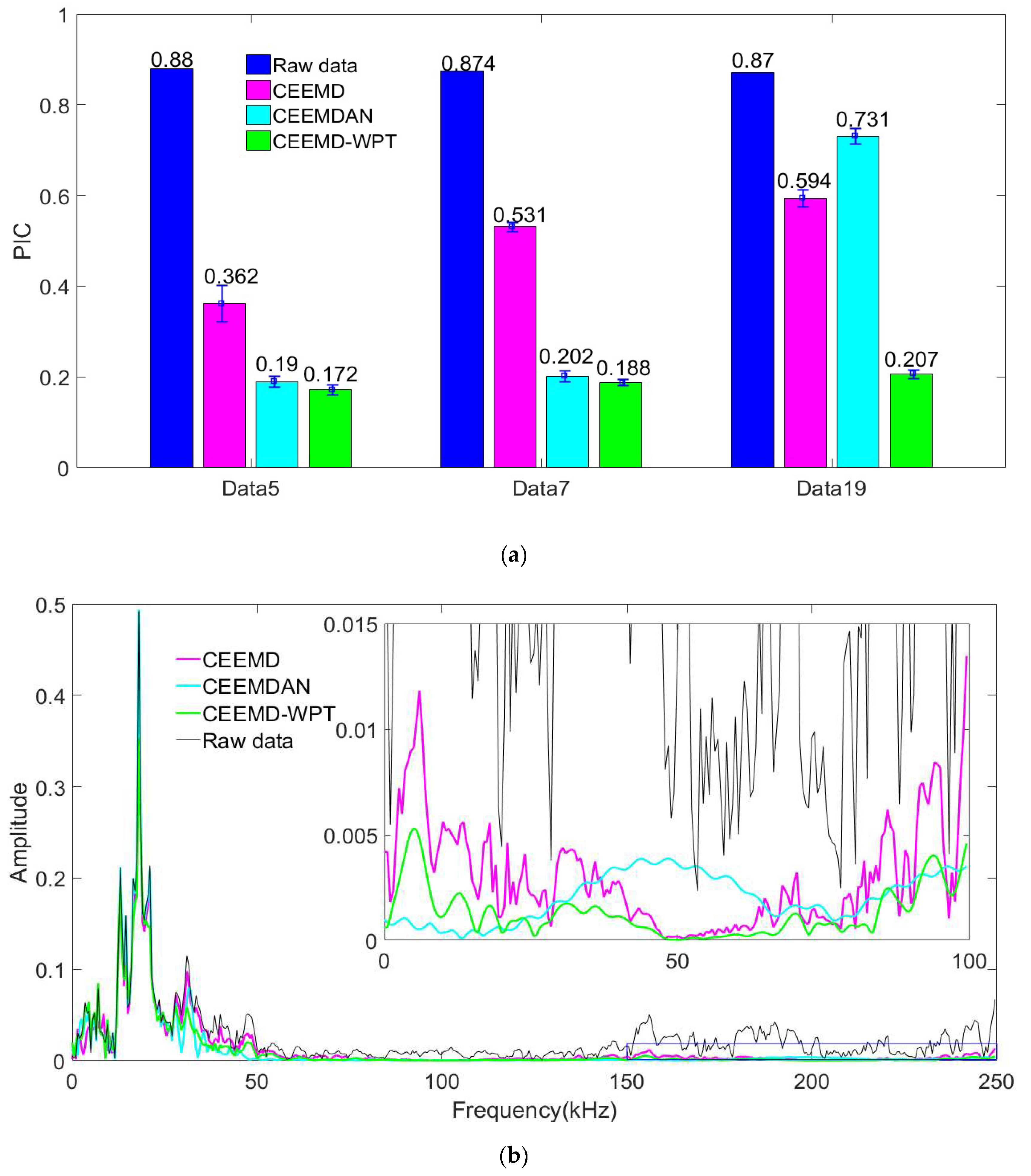
5. Experiment and Analysis

In order to verify the actual noise reduction effect of the proposed method, the Acoustic Event Dataset [30] provided by HARVARD Dataverse was adopted for the noise reduction experiment. The dataset, as shown in Figure 7, has a total of 16,650 AE data, including 15,000 data in the training set and 1650 data in the test set. The data categories are divided into stretch, shear, and mixed events, each accounting for 1/3. The sample number is 1000.

Firstly, a noise reduction experiment was conducted on 1650 pieces of data in the test set, and the PIC index of the original signal, traditional CEEMD, CEEMDAN, and CEEMD-WPT were calculated, respectively. As shown in Figure 8, the PIC index distribution of the original signal is relatively dispersed, mainly ranging from 0 to 0.4. This is because some of the original signals contain noise, which increases their PIC index, and a small number of signals have a large noise content, making their PIC index as high as 0.8–1. After the three noise reduction methods, the PIC index showed a decreasing trend, among which the signals of traditional CEEMD, CEEMDAN, and CEEMD-WPT concentrated in the range of 0–0.2 were 84.9%, 81.9%, and 92.9%, respectively. This shows that CEEMD-WPT has the strongest noise cancellation capability compared to other algorithms, and can reduce the PIC index of most data in the test set to 0–0.2.

Secondly, the test set signal is divided into four intervals according to the PIC index, which are: [0.2–0.4], [0.4–0.6], [0.6–0.8], and [0.8–1]. Traditional CEEMD, CEEMDAN, and CEEMD-WPT denoising were carried out for these four intervals, respectively. The PIC index after denoising was calculated and the results are shown in Figure 9 and

Table 3. PIC interval noise reduction.

	PIC Mean
	0.2–0.4	0.4–0.6	0.6–0.8	0.8–1
Traditional CEEMD	0.173	0.192	0.213	0.454
CEEMDAN	0.181	0.253	0.301	0.323
CEEMD-WPT	0.183	0.182	0.167	0.146

.

By observing Figure 9 and Table 3, it can be found that the CEEMD-WPT algorithm has the best noise reduction effect for signals with a PIC between [0.4 and 1]. For a signal with a PIC between [0.2 and 0.4], the traditional CEEMD has a better noise reduction effect. As a whole, CEEMD-WPT has a wider range of adaptations, so the noise reduction effect is better than traditional CEEMD and CEEMDAN.

In the observation interval [0.8–1] alone, it can be found that the noise reduction effect in order from high to low is CEEMD-WPT, CEEMDAN, and traditional CEEMD, which is consistent with the experimental results in

Table 4. Comparison of experimental results.

	Algorithm	PIC Mean	Variance (10−2)
Test set for all data	Primary signal	0.288
	Traditional CEEMD	0.169
	CEEMDAN	0.159
	CEEMD-WPT	0.156
Data5	Primary signal	0.88
	Traditional CEEMD	0.362	0.158
	CEEMDAN	0.190	0.016
	CEEMD-WPT	0.172	0.013
Data7	Primary signal	0.874
	Traditional CEEMD	0.531	0.010
	CEEMDAN	0.202	0.016
	CEEMD-WPT	0.188	0.005
Data19	Primary signal	0.87
	Traditional CEEMD	0.594	0.034
	CEEMDAN	0.731	0.031
	CEEMD-WPT	0.207	0.009

.

Finally, for the data with more noise in the first 20 pieces of data in the test set (the principal interval coefficient is greater than 0.8 and there are 3 pieces of data, which are the 5th, 7th, and 19th pieces of data, respectively), the noise reduction effect and algorithm stability are observed, and 100 noise reduction experiments are conducted on them, respectively. The noise reduction results are shown in Figure 10, and the data are collected in Table 4.

By observing Figure 10a, it can be found that all three methods can reduce the PIC index, but the PIC index of traditional CEEMD is still high after noise reduction. The PIC index of signal 7 and signal 19 is more than 0.5, and the PIC index has a large fluctuation, which proves that the noise reduction effect is limited and the noise reduction stability is poor. Although the CEEMDAN algorithm has a good effect on Data5 and Data7, it has a poor effect on Data19. On the contrary, the PIC index of CEEMD-WPT after noise reduction is about 0.2 with a small fluctuation, which proves that the proposed method has a better noise reduction effect and stability.

By comparing Figure 10b–d, it can be seen that the three methods have the effect of removing high-frequency noise from the original signal, but compared with CEEMD-WPT, traditional CEEMD has more residual noise in the high-frequency part, which is also the reason for its higher PIC index. The high-frequency noise residue of CEEMDAN on Data19 is obviously higher than that of Data5 and Data7, which is also consistent with the poor noise reduction effect on Data19.

By observing Table 4, it can be found that the PIC index of CEEMD-WPT in the three experimental signals is smaller than that of traditional CEEMD and CEEMDAN, and the variance is significantly smaller than that of traditional CEEMD by one order of magnitude. The stronger stability of the noise reduction effect is mainly attributed to the following two aspects. On the one hand, due to the randomness of white noise added in traditional CEEMD and CEEMDAN, the noise reduction effect has unstable factors, while CEEMD-WPT uses the WPT-EMD method with a more stable noise reduction effect instead of the original single EMD, so the noise reduction results are more stable. On the other hand, white noise added in traditional CEEMD and CEEMDAN smoothed the mutation points and polluted the non-mutation points at the same time, changing the non-mutation points from a low-frequency signal to a high-frequency signal. However, the effect of white noise on non-mutation points could be reduced by using WPT to filter out high-frequency noise before EMD. Thus, the noise reduction capability of the algorithm is improved.

6. Conclusions

(1)

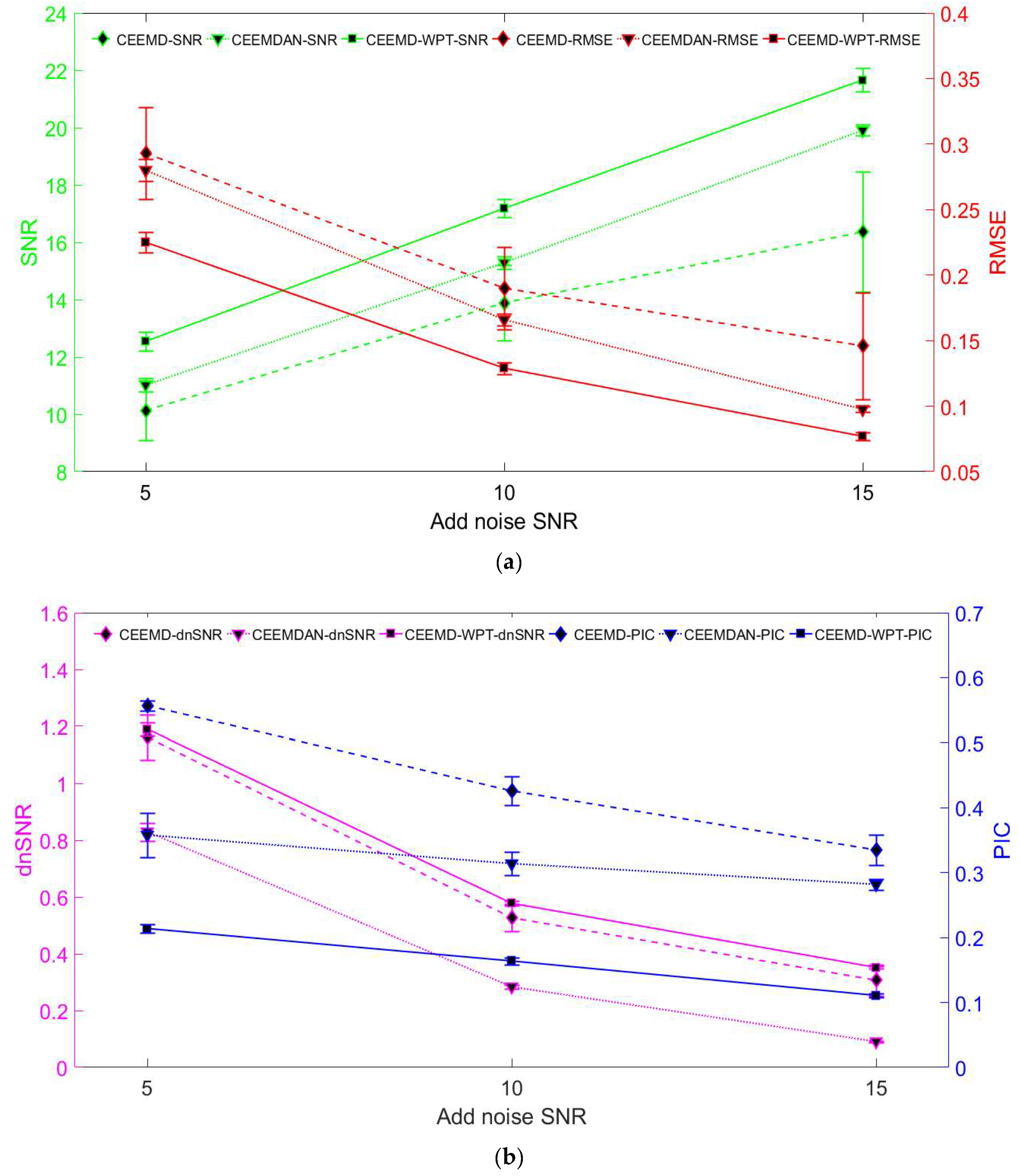
In order to solve the problem of the poor noise reduction effect and the stability of the traditional CEEMD noise reduction algorithm, this paper designed the CEEMD-WPT noise reduction method, and verified the performance of the algorithm by using analog signals and an AE open dataset “Acoustic Event Dataset”. The results show that, compared with traditional CEEMD and CEEMDAN, CEEMD-WPT has the best noise reduction effect and the least noise residue. Moreover, the statistical variance in noise reduction of CEEMD-WPT is one order of magnitude smaller than that of traditional CEEMD, and it has greater stability.

(2)

In order to solve the problem of the noise reduction effect of real signals being difficult to quantify, the PIC index is designed according to the law of noise distribution. In the simulation signal test, it is proved that the PIC index has the same quantization reliability as the SNR and RMSE, and the quantization effect of the dnSNR is poor.

References

1. Jierula, A.; Oh, T.-M.; Wang, S.; Lee, J.-H.; Kim, H.; Lee, J.-W. Detection of damage locations and damage steps in pile foundations using acoustic emissions with deep learning technology. Front. Struct. Civ. Eng. 2021, 15, 318–332. [Google Scholar] [CrossRef]
2. Ma, J.; Dong, L.; Zhao, G.; Li, X. Discrimination of seismic sources in an underground mine using full waveform inversion. Int. J. Rock Mech. Min. Sci. 2018, 106, 213–222. [Google Scholar] [CrossRef]
3. Madarshahian, R.; Ziehl, P.; Caicedo, J.M. Acoustic emission Bayesian source location: Onset time challenge. Mech. Syst. Signal Process. 2019, 123, 483–495. [Google Scholar] [CrossRef]
4. Schabowicz, K. Non-Destructive Testing of Materials in Civil Engineering. Materials 2019, 12, 3237. [Google Scholar] [CrossRef] [PubMed]
5. Kek, T.; Potočnik, P.; Misson, M.; Bergant, Z.; Sorgente, M.; Govekar, E.; Šturm, R. Characterization of Biocomposites and Glass Fiber Epoxy Composites Based on Acoustic Emission Signals, Deep Feature Extraction, and Machine Learning. Sensors 2022, 22, 6886. [Google Scholar] [CrossRef] [PubMed]
6. Supriyo, M.; Piyush, S.; Ramesh, B.N. A robust condition monitoring methodology for grinding wheel wear identification using Hilbert Huang transform. Precis. Eng. 2021, 70, 77–91. [Google Scholar]
7. Ohtsu, M. Acoustic Emission (AE) and Related Non-Destructive Evaluation (NDE) Techniques in the Fracture Mechanics of Concrete; Elsevier Ltd.: Amsterdam, The Netherlands, 2015. [Google Scholar]
8. Xiao, P.; Hu, Q.; Tao, Q.; Dong, L.; Yang, Z.; Zhang, W. Acoustic Emission Location Method for Quasi-Cylindrical Structure With Complex Hole. IEEE Access 2020, 8, 35263–35275. [Google Scholar] [CrossRef]
9. Ohtsu, M. Recommendation of RILEM TC 212-ACD: Acoustic emission and related NDE techniques for crack detection and damage evaluation in concrete: Test method for classification of active cracks in concrete structures by acoustic emission. Mater. Struct. 2010, 43, 1187–1189. [Google Scholar]
10. Eline, V.; Menno, V.D.V.; Edwin, R.; Lombaert, G.; Verstrynge, E. Experimental study on acoustic emission sensing and vibration monitoring of corroding reinforced concrete beams. Eng. Struct. 2023, 293, 116553. [Google Scholar]
11. Tayfur, S.; Alver, N.; Abdi, S.; Saatcı, S.; Ghiami, A. Characterization of concrete matrix/steel fiber de-bonding in an SFRC beam: Principal component analysis and k-mean algorithm for clustering AE data. Eng. Fract. Mech. 2018, 194, 73–85. [Google Scholar] [CrossRef]
12. Kononenko, D.Y.; Nikonova, V.; Seleznev, M.; van den Brink, J.; Chernyavsky, D. An in situ crack detection approach in additive manufacturing based on acoustic emission and machine learning. Addit. Manuf. Lett. 2023, 5, 100130. [Google Scholar] [CrossRef]
13. Chen, L.; Yao, X.; Tan, C.; He, W.; Su, J.; Weng, F.; Chew, Y.; Ng, N.P.H.; Moon, S.K. In-situ crack and keyhole pore detection in laser directed energy deposition through acoustic signal and deep learning. Addit. Manuf. 2023, 69, 103547. [Google Scholar] [CrossRef]
14. González, D.; Alvarez, J.; Sánchez, J.A.; Godino, L.; Pombo, I. Deep Learning-Based Feature Extraction of Acoustic Emission Signals for Monitoring Wear of Grinding Wheels. Sensors 2022, 22, 6911. [Google Scholar] [CrossRef] [PubMed]
15. Liu, Z.; Zhou, Y.; Zou, S.; Zhang, X. Research on noise reduction method of Hydraulic turbine cavitation acoustic emission signal with improved threshold wavelet. J. Hydroelectr. Power 2019, 45, 85–89+98. (In Chinese) [Google Scholar]
16. Hassan, F.; Rahim, L.A.; Mahmood, A.K.; Abed, S.A. A Hybrid Particle Swarm Optimization-Based Wavelet Threshold Denoising Algorithm for Acoustic Emission Signals. Symmetry 2022, 14, 1253. [Google Scholar] [CrossRef]
17. He, K.; Xia, Z.; Si, Y.; Lu, Q.; Peng, Y. Noise Reduction of Welding Crack AE Signal Based on EMD and Wavelet Packet. Sensors 2020, 20, 761. [Google Scholar] [CrossRef]
18. Hu, L.; Gao, H.; Shi, D.; Lin, Z.; Li, K.; Zhao, L. Noise reduction method of mechanical seal acoustic emission signal based on CEEMD and improved wavelet threshold. Comput. Meas. Control 2019, 27, 157–161+166. (In Chinese) [Google Scholar]
19. Sun, Y.; Wang, L.; Lei, Q.; Cao, Q. Research on Vibration Prediction of Hydropower Unit Based on CEEMDAN-IPSO-LSTM [J/OL]. The People of the Yellow River: 1-7 [2023-03-21]. Available online: http://kns.cnki.net/kcms/detail/41.1128.TV.20230309.1022.002.html (accessed on 17 April 2023). (In Chinese).
20. Zhang, J.; Dong, L.; Xu, N. Noise Suppression of Microseismic Signals via Adaptive Variational Mode Decomposition and Akaike Information Criterion. Appl. Sci. 2020, 10, 3790. [Google Scholar] [CrossRef]
21. Jing, G.; Zhao, Y.; Gao, Y.; Marin Montanari, P.; Lacidogna, G. Noise Reduction Based on Improved Variational Mode Decomposition for Acoustic Emission Signal of Coal Failure. Appl. Sci. 2023, 13, 9140. [Google Scholar] [CrossRef]
22. Chen, N.; Sun, H.; Zhang, Q.; Li, S. A Short-Term Wind Speed Forecasting Model Based on EMD/CEEMD and ARIMA-SVM Algorithms. Appl. Sci. 2022, 12, 6085. [Google Scholar] [CrossRef]
23. Yang, Z.; Lin, J.; Wang, K.; Cheng, X.; Liu, P. Research on noise reduction of concrete acoustic emission Signal based on CEEMDAN-Wavelet packet adaptive threshold. Vib. Shock. 2023, 3, 139–149. (In Chinese) [Google Scholar]
24. Luan, X.; Li, Y.; Xu, S.; Sha, Y. Fault diagnosis method of rolling bearing based on wavelet packet transform and CEEMDAN [J/OL]. J. Air Power 2023, 3, 1–16. (In Chinese) [Google Scholar] [CrossRef]
25. Yu, H.; Wen, H.; Liu, H.; Dong, J.; Lin, W. GNSS elevation time series denoising method based on CEEMDAN and wavelet packet multi-threshold. Geod. Geodyn. 2022, 10, 1005–1009. (In Chinese) [Google Scholar]
26. Meng, J.; Han, Z.; Li, Y. Adaptive wavelet entropy threshold seismic random noise suppression algorithm based on improved complementary set empirical mode decomposition. Sci. Technol. Eng. 2019, 19, 52–61. (In Chinese) [Google Scholar]
27. Yi, J.; An, H.; Xing, Y.; Li, J.; Zhang, G.; Bamisile, O.; Yamg, K.; Xu, Y. A cyber attack detection strategy for plug-in electric vehicles during charging based on CEEMDAN and Broad Learning System. Energy Rep. 2023, 9, 80–88. [Google Scholar] [CrossRef]
28. Yu, J.; Zhao, S.; Wang, Q. Acoustic emission signal denoising based on empirical mode decomposition and wavelet transform. J. Harbin Inst. Technol. 2011, 43, 88–92. (In Chinese) [Google Scholar]
29. Mitraković, D.; Grabec, I.; Sedmak, S. Simulation of AE signals and signal analysis systems. Ultrasonics 1985, 23, 227–232. [Google Scholar] [CrossRef]
30. Siracusano, G. Acoustic Event Dataset; Harvard Dataverse: Cambridge, MA, USA, 2019. [Google Scholar] [CrossRef]
Figure 1. Flow chart of improved CEEMD-WPT noise reduction method.
Applsci 13 10274 g001
Figure 2. Analog signal: (a) Analog signal waveform diagram. (b) Analog signal spectrum diagram.
Applsci 13 10274 g002aApplsci 13 10274 g002b
Figure 3. Expanded view of noisy signals.
Applsci 13 10274 g003
Figure 4. Distribution of correlation numbers.
Applsci 13 10274 g004
Figure 5. The noise reduction effect of a noisy signal: (a) Noise reduction rendering of traditional CEEMD. (b) CEEMDAN noise reduction effect diagram. (c) Noise reduction effect diagram of CEEMD-WPT. (d) Noise reduction spectrum map of traditional CEEMD. (e) CEEMDAN noise reduction spectrum map. (f) Noise reduction spectrum map of CEEMD-WPT.
Applsci 13 10274 g005aApplsci 13 10274 g005bApplsci 13 10274 g005c
Figure 6. Comparison of noise reduction quantization parameters: (a) SNR-RMSE; (b) dnSNR-PIC.
Applsci 13 10274 g006
Figure 7. Schematic representation of Acoustic Event Dataset.
Applsci 13 10274 g007
Figure 8. Denoising diagram of test set signal.
Applsci 13 10274 g008
Figure 9. PIC interval noise reduction diagram: (a) 0.2–0.4; (b) 0.4–0.6; (c) 0.6–0.8; (d) 0.8–1.
Applsci 13 10274 g009aApplsci 13 10274 g009bApplsci 13 10274 g009c
Figure 10. Noise reduction figures of Data5, 7, and 19: (a) All Data. (b) Data5. (c) Data7. (d) Data19.
Applsci 13 10274 g010aApplsci 13 10274 g010b