A Decision-Fusion-Based Ensemble Approach for Malicious Websites Detection

Abstract

Malicious websites detection is one of the cyber-security tasks that protects sensitive information such as credit card details and login credentials from attackers. Machine learning (ML)-based methods have been commonly used in several applications of cyber-security research. Although there are some methods and approaches proposed in the state-of-the-art studies, the advancement of the most effective solution is still of research interest and needs to be improved. Recently, decision fusion methods play an important role in improving the accuracy of ML methods. They are broadly classified based on the type of fusion into a voting decision fusion technique and a divide and conquer decision fusion technique. In this paper, a decision fusion ensemble learning (DFEL) model is proposed based on voting technique for detecting malicious websites. It combines the predictions of three effective ensemble classifiers, namely, gradient boosting (GB) classifier, extreme gradient boosting (XGB) classifier, and random forest (RF) classifier. We use these classifiers because their advantages to perform well for class imbalanced and data with statistical noises such as in the case of malicious websites detection. A weighted majority-voting rule is utilized for generating the final decisions of used classifiers. The experimental results are conducted on a publicly available large dataset of malicious and benign websites. The comparative study exposed that the DFEL model achieves high accuracies, which are 97.25% on average of 10-fold cross-validation test and 98.50% on a holdout of 30% test set. This confirms the ability of proposed approach to improve the detection rate of malicious websites.

1. Introduction

With the growing number of mobile devices, web applications, and users, as well as the prompt evolution of computing, cyber-security has become critical in recent years [1]. Easy access to the computer networks and Internet applications, the accessibility of high-speed networks, and high-industrial advancements such as the development of 5G and 4G technologies, have comprehensively expanded Internet usage worldwide [2]. In particular, as a result of the recent improvements in information technology and digitalization, several enterprises and companies have shifted their businesses from the physical to digital domain, employing mobile and web applications to decrease physical contact [3,4]. However, this growth in Internet applications and websites has caused them to become significantly open and accessible to the rest of the world and comes with a significant security risk and a leakage of private data.

Because of the easy access to the Internet, a person’s digital visibility has extensively increased, creating opportunities for digital thieves and hackers to gain access to private data and credentials. Detecting malicious integrity attacks and protecting transmitted data from eavesdropping attacks are critical to prevent user information from being manipulated or destroyed in the integrated data-driven framework [5]. Such cyber-security breaches lead to severe mental stress and financial losses over time [6]. Malicious websites are considered the means by which the hackers can collect private information from unsuspecting Internet consumers. Malicious websites normally appear to be benign websites and request private information, such as passwords, usernames, and credit card information, or gain access to personal images or crucial data. Such data are stored in a form of data storage and might be exploited to achieve the attackers’ goals, such as criminal money transfers, online shopping, harassing the user, or blackmailing. Using forged webpages identical to genuine webpages is a common method to steal users’ data and private information [7].

One method of ensuring user security is to use classification techniques to determine whether the accessed website is malicious [8,9]. A correct classification ensures that the user is informed to not enter his/her data and important information on suspect websites [10,11]. Recently, machine learning methods have demonstrated exceptional results by using data classification [12,13]. They are not only used for malicious websites and attack detection, but are also applied in numerous identification, classification, and prediction tasks in a variety of fields, such as stock prediction [14], weather prediction [15], and image processing [16]. The machine learning field has shown much progress and promise, with large amounts of data becoming available, the development of advanced computational models, and advancements in computing power. Traditional machine learning methods begin with building a new model architecture, followed by the initialization of its parameters. The model is then trained with the training set to learn the relationship between the features of the inputs and the actual class outputs. After that, the model can be validated in the training stage by computing its results on a validation set, which is known as the validation stage. A trained model is then tested on unseen instances, and the classification results are obtained to assess its performance. Support Vector Machine (SVM) [17], K-Nearest Neighbors (KNN) [18], Decision Tree (DT) [19], Naïve Bayes (NB) [20], and Logistic Regression (LR) [21] are some common machine learning methods.

In the literature, some evaluation metrics, such as precision, accuracy, recall, and F1-score, are applied to evaluate the machine learning outputs [22]. These evaluation metrics are mathematically computed based on the confusion matrices, in which true positives, false positives, true negatives, and false negatives are counted. Then, a defined formula using the ratio of the two true and two false amounts can be utilized to assess a model’s performance on a particular data set. One of the main issues encountered during machine learning data classification in general [23,24], and more specifically in malicious websites’ classification [25], is the class-imbalanced dataset. In the class-imbalanced issue, a number of classes or a specific class can contain a more instances than another class or group of classes. This means that, in th training stage, the machine learning method becomes biased toward this specific class or other classes with a large number of instances. This can produce a high result for the dominating class or classes, with the results of other classes being completely disregarded. A number of data-balancing strategies are suggested in the literature. Some common strategies are under-sampling, SMOTE, and over-sampling, which have generally been used for imbalanced data classification [26], and specifically for malicious websites classification [25]. However, the biases in the original dataset of malicious websites might keep the data balanced. Moreover, quality assurance in data-balancing is expensive work, and finding an effective data-balancing method is a challenging task, which must prevent overlap between synthesized samples of classes [27].

In this research work, we propose a decision-fusion-based approach that builds a decision-fusion ensemble learning (DFEL) model by combining the decisions of three effective ensemble classifiers, namely, a gradient boosting (GB) classifier, extreme gradient boosting (XGB) classifier, and random forest (RF) classifier. The approach exploits the advantages of these classifiers when used for for class-imbalanced data and data with statistical noise, as in the case of malicious website detection. We utilize a weighted majority-voting rule to generate the final decisions of developed model. The main contributions of the proposed approach can be summarized as follows:

• Improving the accuracy of malicious website detection by exploiting the diversity of boosting (i.e., GB and XGB) and bagging (i.e., RF) techniques. In boosting, the approach can create sequential models by combining weak learners into strong learners, where the final model has the highest accuracy. Furthermore, in bagging, the approach can create different training subsets from a sample training set using replacement and the output of the final model is based on the majority voting.
• Reducing the class-imbalanced and over-fitting problems in malicious website classification due to the regularization ability of GB, XGB, and RF classifiers.
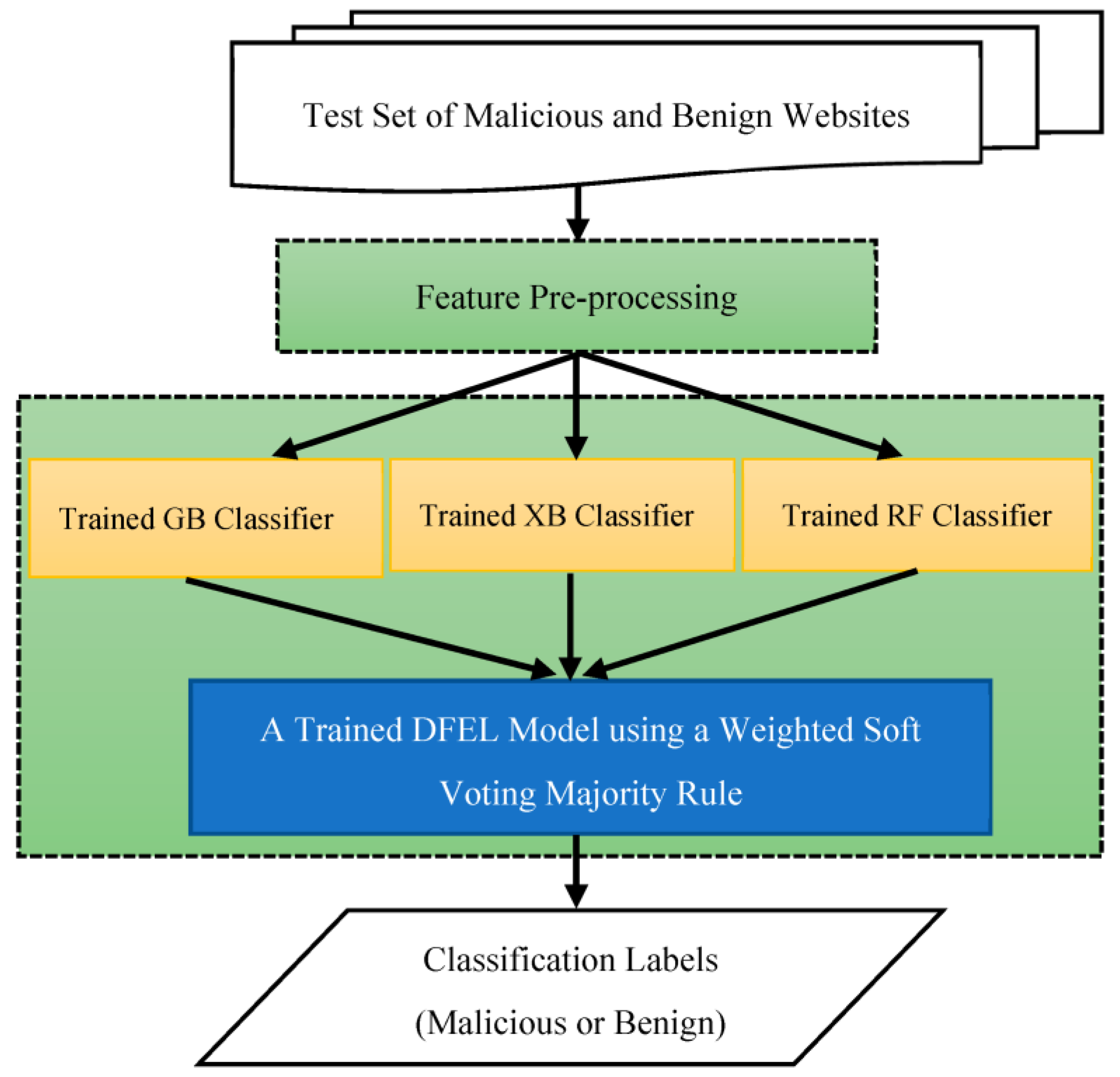
• Proposing a weighted soft voting rule to fuse the final classification scores utilizing the competence of well-calibrated and diverse classifiers such as the base classifiers in the approach. Furthermore, evaluating and comparing the accuracy of the proposed DFEL model with its base classifiers and some recent related work.

The rest of the paper is organized as follows: Section 2 presents the methods and approaches of the related work. Section 3 offers an explanation of the materials and methods used in the research work, including a description of the dataset, methods of the proposed approach, and evaluation metrics. The experiments and results, along with a discussion, are introduced in Section 4. Section 5 summarizes the conclusions and future work.

2. Related Work

Singhal et al. [28] classified malicious and benign websites using supervised machine learning classifiers such as decision trees, random forest, deep neural network, and gradient boosting. First, the authors gathered the URLs. Then, they extract host-based, lexical-based, and content-based features from malicious and benign websites. These features were used as the inputs to machine learning models. The authors generated the lexical features by choosing the length of host, the length of URL, the length of path, the count of host token, and some other symbols.

Similarly, the autonomous system number (ASN) and location, which are the host-based features, were obtained from the URL. The author chose applet count, HTTPS-enabled, Eval function, redirection, XMLHttpRequest, unescaped function, and popups as the content-based features. The authors obtained the benign websites from PhishTank’s public blacklist. This dataset contains a total of 80,000 unique balanced URLs. The features were extracted after the data were collected. To compare different classifiers, the same measures (precision, accuracy, F1-score, and recall) were used to quantify the classifier results on this dataset. Using the gradient-boosting method, the authors achieved the best accuracy result of 96.4%.

Amrutkar et al. [29] created an analysis technique, named kAYO, to distinguish between benign and malicious mobile websites based on the static features. For classification, their method makes use of the static features of a website. The authors applied the proposed method to a huge, labeled data set of 350,000 benign and malicious mobile websites, and attained 90% accuracy. They created a browser extension for their proposed technique. The kAYO was run in the browser extension’s backend to determine whether selected webpages are benign or malicious.

McGahagan et al. [30] investigated the relation between the number of extracted features from the HTTP headers and the likelihood of malicious webpage detection. They examined 6021 malicious websites’ HTTP headers and 39,853 benign websites’ HTTP headers. The number of features extracted from HTTP headers was 672 and the authors selected 22 features for further analysis; 11 of these features were considered in previous research and the remaining 11 features were used in these authors’ work. Three of the twenty-two features contained 80% of the total importance of these features. The authors conducted a principal component analysis (PCA) of the extracted features and used eight classifiers to improve the detection rate. They found that the 22 features attained a better accuracy result.

A hybrid approach was used by Patil et al. [31] to find malicious URLs. In the hybrid approach, they combined static and dynamic features; the static features were extracted using a static method and the other dynamic features were extracted using a dynamic method. A total of 117 features were extracted; 44 of them were new features. The dataset used in their study comprised 52,082 samples. The training data contained a total of 40,082 instances: 20,041 instances in the malicious class and 20,041 in the benign class. This demonstrates that the authors’ study’s dataset is balanced. The authors used six machine learning methods, including the simple CART, DT, RF, ADTree, random tree (RT), and REPTree, to assess the effectiveness of their approach.

A one-dimensional convolutional neural network (1D-CNN) architecture was proposed by Al-milli et al. [32] to detect benign URLs. The experiment wasconducted by the authors using a benchmark dataset and receiver operating characteristic (ROC) curve with accuracy evaluation metrics. The authors collected 2456 records with 30 features in their dataset. A total of 70% of the dataset was applied for training, and 30% was utilized for testing. They built a CNN architecture containing 64 filters and 16 kernel sizes with 500 and 2000 epochs. The authors’ model achieved a 91.23% area under the curve (AUC) and 94.31% accuracy.

A two-step method for the detection of benign and malicious URLs was introduced by Jayakanthan et al. [33]. An algorithm called “enhanced probing classification of malicious URLs (EPCMU)” is used as the first step and an NB classifier is used as the second step to find malicious URLs. The first step involves the detection task and the second is used for classification. The input URLs are thoroughly examined by the EPCMU. The system flags the URLs as malicious if they exhibit any characteristics of a malicious websites or appear on the blacklisted websites. Otherwise, more checks ar eperformed. In the EMPCU, a collection of URLs serves as input to the NB classifier during the classification stage. This determines whether the set URLs are genuine or malicious.

An auto-encoder model was used by Assefa et al. [34] to differentiate between benign and malicious websites. Three layers (input, hidden, and output) make up the structure of the auto-encoder model. The data of legitimate webpages were gathered from the dataset created by the Canadian Institute for Cyber-security, while the phishing data of webpages were gathered from the dataset generated by the open-source Phish Tank. The final dataset contained a total of 16 features and 10,000 instances. The authors cleaned the missing extracted values in the preprocessing stage. The effectiveness of the auto-encoder-based model is compared to DT and SVM. The authors’ model attained 91.24% accuracy. The DT and SVM methods delivered an accuracy of 86.1% and 88.4%, respectively.

The contributions and results of important related research have confirmed the ability and applicability of these methods and techniques for detecting benign and malicious websites. Recently, Hassan et al. [25] proposed an approach using DT, RF, SVC, LR, and Stochastic Gradient Decent (SGD) classifiers and achieved 94.19% accuracy for imbalanced datasets. The results for data balancing in [25] are discarded because the authors balanced the dataset before splitting it into training and test sets. This means that the distribution of augmented instances in the test set has almost the same distribution of original instances in the training set and increases the accuracy. Singhal et al. [28] applied RF, GB, DT, and deep neural network (DNN) methods to obtain an accuracy of up to 96.4%. Amrutkar et al. [29] achieved 90% accuracy using the kAYO technique. Adaptive Boosting (AB), Extra Trees (ET), RF, GB, Bagging Classifier (BC), LR, and k-NN were used by McGahagan et al. [30] to obtain an accuracy of up to 89%. Al-milli et al. [32] proposed an approach using a 1D-CNN to attain 94.31% accuracy. Assefa et al. [34] used an auto-encoder, DT, and SVM to attain 91.24% accuracy. Sandag et al. [35] applied the k-NN method to website features and attained 95% accuracy. Alkhudair et al. [36] and Panischev et al. [37] proposed methods using RF to obtain 95% accuracy for both studies. Labhsetwar et al. [38] achieved 92% accuracy by using an RF classifier. Singh et al. [39] proposed a multilayer CNN and attained an accuracy of 91%. Aljabri et al. [40] used an NB classifier and 96% accuracy was obtained. Utku and Can [41] proposed an approach using LightGBM, DT, SVM, k-NN, LR, multilayer perceptron (MLP), RF, and XGB to gain 96% accuracy.

The results of previous studies show that the existing methods have several strengths, such as a good performance on malicious website detection tasks. They are simple and can be regularized to decrease the chance of over-fitting. Their outputs can be interpreted easily, and some of them do not need to scale the feature values and can be used for both non-linear and linear features. However, they have limitations in their ability to produce an effective trained model with reduced variance and bias, and improved classification results. Moreover, a common limitation of the existing work is the ability to reduce the effect of class-imbalanced and highly correlated features on the accuracy and performance of malicious website classification. These limitations are still a research gap that needs to be solved.

3. Materials and Methods

This section first describes the benchmark data set utilized for building and evaluating the proposed classification model. Next, the methods of the proposed approach are explained. Finally, we describe the proposed approach, including its steps, in detail.

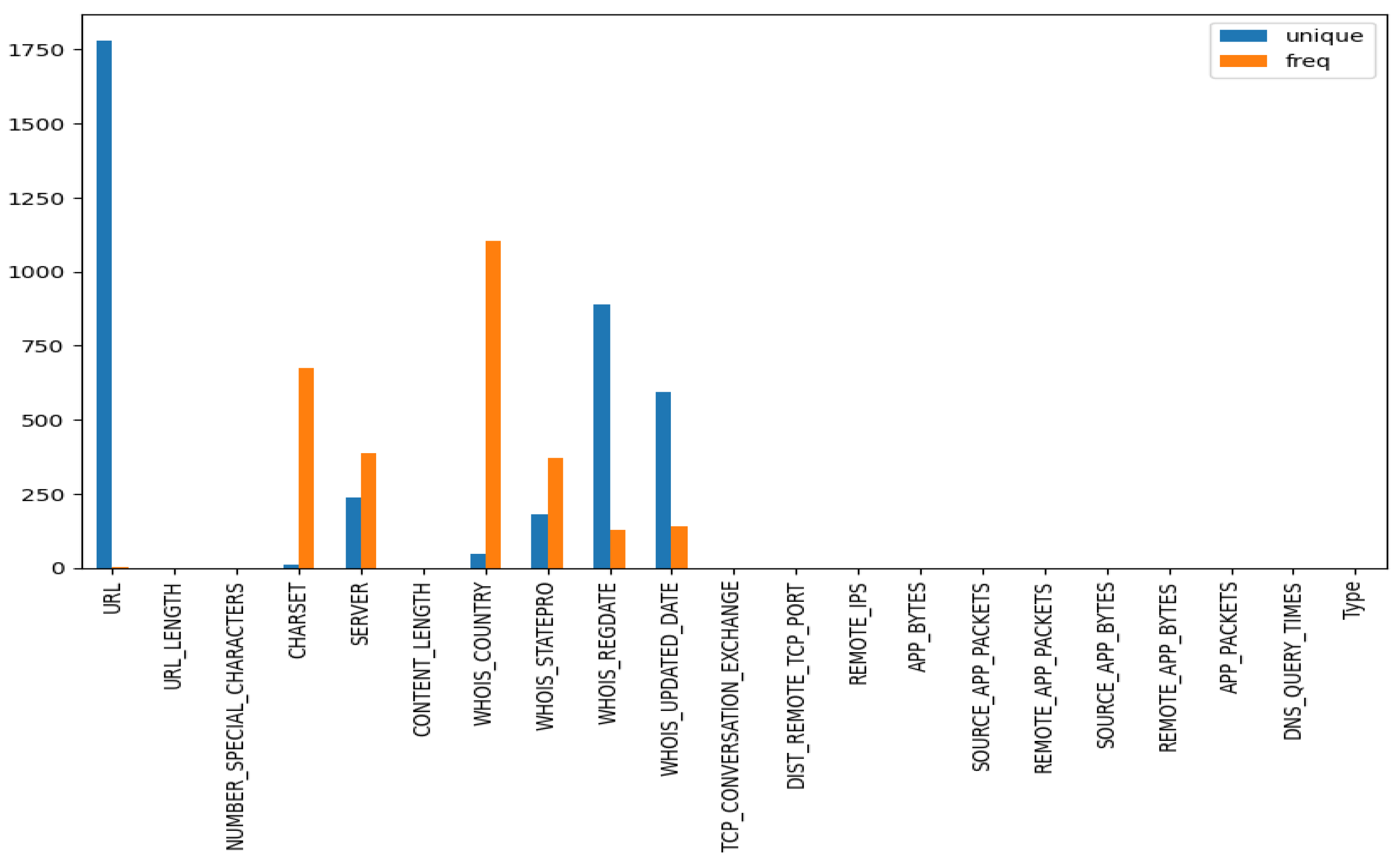
3.1. Benchmark Dataset of Study

The dataset adopted in this research is available on the Kaggle platform, https://www.kaggle.com/datasets/xwolf12/malicious-and-benign-websites (accessed on 15 June 2023). It is a public dataset. It contains 1781 rows of data instances and 21 columns of variables (features) for benign and malicious websites. The target label is the ‘Type’ column, which indicates if the example data are for a benign or malicious website. The features of websites, with their data type included in the dataset, are presented in

Table 1. Features of the dataset and the data types.

No.	Feature	Data Type
0	URL	object
1	URL_LENGTH	int64
2	NUMBER_SPECIAL_CHARACTERS	int64
3	CHARSET	object
4	SERVER	object
5	CONTENT_LENGTH	float64
6	WHOIS_COUNTRY	object
7	WHOIS_STATEPRO	object
8	WHOIS_REGDATE	object
9	WHOIS_UPDATED_DATE	object
10	TCP_CONVERSATION_EXCHANGE	int64
11	DIST_REMOTE_TCP_PORT	int64
12	REMOTE_IPS	int64
13	APP_BYTES	int64
14	SOURCE_APP_PACKETS	int64
15	REMOTE_APP_PACKETS	int64
16	SOURCE_APP_BYTES	int64
17	REMOTE_APP_BYTES	int64
18	APP_PACKETS	int64
19	DNS_QUERY_TIMES	float64
20	Type	int64

. Figure 1 demonstrates the number of dataset instances for the benign and malicious classes and their distribution. As shown in Figure 1, the distribution of instances in the dataset is imbalanced, as the malicious class form 87.9% of the total, while 12.1% are benign.

During the collection process and analysis of the dataset, features were collected from the network and application layers to enable the use of static and dynamic website characteristics. A description of each feature in the dataset is provided as follows:

• The URL is a unique identification of the Uniform Resource Locators (URLs), analyzed in the collected dataset.
• The ‘URL_LENGTH’ is the number of characters in the URL.
• The ‘NUMBER_SPECIAL_CHARACTERS’ is the number of special characters in the URL.
• The ‘CHARSET’ is a character set that has a categorical value that represents the character encoding standard.
• The ‘SERVER’ is a categorical value that represents the server operative system extracted from the packet response.
• The ‘CONTENT_LENGTH’ is the HTTP header content size.
• The ‘WHOIS_COUNTRY’ indicates the country in which the website server is situated.
• The ‘WHOIS_STATEPRO’ represents the location at which the website is registered.
• The ‘WHOIS_REGDATE’ is the registration date of the website server.
• The ‘WHOIS_UPDATED_DATE’ is the date of the last update to the website server.
• The ‘TCP_CONVERSATION_EXCHANGE’ counts the number of packets between the honeypot and website using the TCP protocol.
• The ‘DIST_REMOTE_TCP_PORT’ is the total number of ports, rather than those exposed in TCP.
• The ‘REMOTE_IPS’ is the total number of Internet Protocols (IPs) in the connection of the honeypots.
• The ‘APP_BYTES’ is the number of transferred bytes.
• The ‘SOURCE_APP_PACKETS’ is the number of packets that were directed from the honeypot to the server.
• The ‘REMOTE_APP_PACKETS’ is the number of packets that arrived from the server.
• The ‘SOURCE_APP_BYTES’ is the number of bytes that were directed from the honeypot to the server.
• The ‘REMOTE_APP_BYTES’ is the number of bytes that arrived from the server.
• The ‘APP_PACKETS’ is the total number of IP packets produced through the communication between honeypot and server.
• The ‘DNS_QUERY_TIMES’ is the number of DNS packets produced through the communication between honeypot and server.
• The ‘Type’ is a categorical variable that represents the class name of the analyzed website; specifically, 0 denotes a benign website and 1 a malicious website.

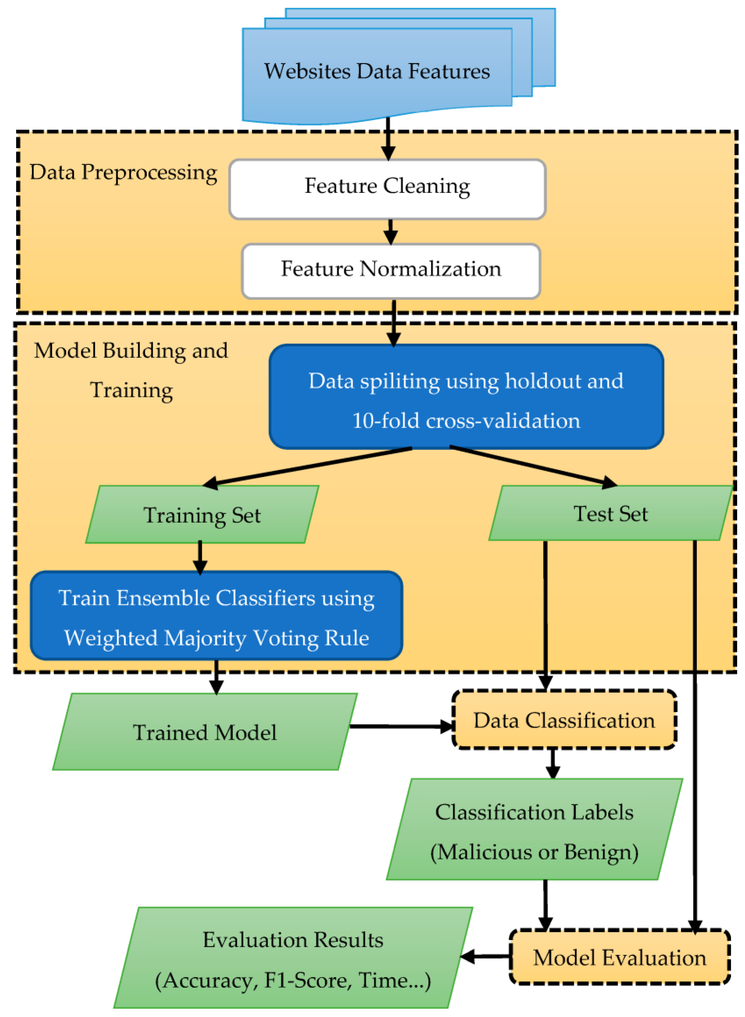
3.2. Methodology of Proposed Approach

3.2.1. Gradient-Boosting (GB) Classifier Method

Gradient-boosting (GB) is a supervised learning method. It is used in many applications for regression and classification tasks. GB combines several weak learners to produce a strong predicative model. This process is called an ensemble of weak learners, which are usually decision trees [42,43].

Conceptually, ensemble learning uses various classifiers to effectively classify the data instances and aggregate their predictions. The boosting technique [44] is a type of ensemble learning that can resolve classification or regression tasks by fusing several models to build an ensemble model. The error of the combined models is minimized by giving extra weight to the training instances that are incorrectly predicted or classified by previous learners. For the final prediction of the ensemble model, a weighted voting rule is used. GB, as one of the boosting methods, aggregates the prediction results of multiple decision trees to boost the performance of a single tree model [45]. Moreover, GB can improve the performance of datasets with class-imbalance issues [46]. Therefore, it is used in our approach to improve the accuracy of malicious websites detection, especially when suffering from a class-imbalance problem. Algorithm 1 generates several decision trees using training dataset examples and builds the GB classifier.

Algorithm 1. Building GB classifier

Input: A training dataset with $\left(x_1,y_1\right), \dots \left(x_m,y_m\right) where x_i\in X,y_i\in Y;$ T is the number of random trees using distribution $D_t$. Output: The final decision tree (GB classifier). Begin 1. For t = 1 to T. 1.1. $\mathrm{Initializing} D_1\left(i\right)=\frac{1}{m};$ 1.2. $\mathrm{Calculating} \mathrm{the} \mathrm{hypothesis} h_t:X\to \left\{-1,+1\right\}$ 1.3. $\mathrm{Calculating} {e_t=P_{r_{i~D_t}}[\mathrm{h}}_t\left(x_i\right)\ne y_i];$ 1.4. $\mathrm{Selecting} \mathrm{a} \mathrm{random} \mathrm{subsample} \mathrm{of} \mathrm{training} \mathrm{dataset} \mathrm{with}{\propto }_t=\ln \ln (\frac{1-e_t}{e_t}).$ 1.5. Updating the model using the selected subsample with $$\begin{gathered} \hspace{1em}\hspace{1em}\hspace{1em}\hspace{1em}\hspace{1em}\hspace{1em}\hspace{1em}{D}_{t+1}\left(i\right)=\frac{D_t\left(i\right)}{Z_t}\times \{e^{-\propto t}\}if {\mathrm{h}}_t\left(x_i\right)=y_i{e^{\propto t}if \mathrm{h}}_t\left(x_i\right)\ne y_i= \\ \hspace{1em}\hspace{1em}\hspace{1em}\hspace{1em}\hspace{1em}\hspace{1em}\hspace{1em}\frac{D_t\left(i\right) \mathrm{e}\mathrm{x}\mathrm{p} (\propto t y_i {\mathrm{h}}_t\left(x_i\right))}{Z_t}, \end{gathered}$$        where $Z_t \mathrm{i}\mathrm{s} \mathrm{a} \mathrm{n}\mathrm{o}\mathrm{r}\mathrm{m}\mathrm{a}\mathrm{l}\mathrm{i}\mathrm{z}\mathrm{a}\mathrm{t}\mathrm{i}\mathrm{o}\mathrm{n} \mathrm{f}\mathrm{a}\mathrm{c}\mathrm{t}\mathrm{o}\mathrm{r}.$ 2. Growing a tree f(x); 3. Adding f(x) to the GB classifier; End

For each iteration of the boosting algorithm, the instances that were incorrectly classified in the previous iterations are adjusted. This can be performed by increasing the weights of misclassified instances and decreasing the weights of correctly classified instances. Therefore, each successive learner focuses on misclassified instances. After finalizing the iterations, the random modified decision trees will be combined by a weighted-majority voting rule to build the final GB classifier.

3.2.2. Extreme Gradient-Boosting (XGB) Classifier Method

Extreme Gradient-Boosting (XGB) is another supervised learning method, developed by Chen Tianqi [47]. In the loss function, the XGB uses a quadratic Taylor expansion and a regularization term is added to reduce over-fitting and to make the classifier simpler. The XGB automatically uses the central processing unit (CPU) and multi-threading for parallelism. At the same, it processes sparse high-dimensional features in a distributed way. This makes the XGB faster and more accurate for different applications than similar methods [48]. The XGB method is an improved version of the gradient-boosting concept and is used for both regression and classification applications [49]. It is a scalable learning method of the boosted-trees-based methods, which is commonly and efficiently applied for large-scale features with a notable effect on parallel boosted-tree operations and a flexible manner. The XGB parameters are separated into three groups, which are boosting parameters, general parameters, and learning parameters. To boost the model, it is recommended that the boosting parameters are optimized. Algorithm 2 shows the steps in building an XGB classifier model.

Algorithm 2. Building XGB classifier model.

Input:$X=\left\{\right(x_1, y_1), (x_2, y_2), \dots , (x_m, y_m\left)\right\}$ is a training samples; $T$ is a maximum number of iterations; max-depth; regularization coefficients, and other parameters. Output: strong learner $f\left(x\right)$;

Begin 1. For t = 1 to T: 2. $\mathrm{Calculate} \mathrm{the} \mathrm{loss} \mathrm{function} \left(L\right)$$\mathrm{of} \mathrm{the} \mathrm{i}\mathit{th} \mathrm{instances} (i=1, 2, \dots , m)$ in the present iteration based on the max-depth, regularization coefficients, and the other parameters. 3. Calculate the first derivative and second derivative of all instances. 4. Split the decision-tree using the score of the processed node; the value 0 is the default score. The score of the node that is subjected to the splitting process is the sum of the first derivative and second derivative. 5. Split the sub-number using the eigenvalue and division feature based on the maximum value. 5.1. If the maximum value is equal to 0, then establish the present decision tree; 5.1.1. Calculate the weights of all leaf regions to generate the weak learner. 5.1.2. Update the strong learner and enter the next iteration of the weak learner. 5.2. If the maximum value is not equal to 0, continue from step 5 to split the decision tree. End

The proposed approach uses the XGB classifier to classify benign and malicious websites, proving to be an effective classifier in the decision fusion ensemble learning (DFEL) model.

3.2.3. Random Forest (RF) Classifier Method

Random Forest is an ensemble-based method. It combines multiple decision trees to improve the accuracy and reduce the over-fitting problem [50]. The algorithm involves two main steps: training and prediction. In the training step, a subset of the training data is randomly selected and, for each subset, a set of features is randomly chosen. Then, a decision tree is built using the selected features and the subset of data. After that, the previous steps are repeated a specified number of times (or until a stopping criterion is met). Finally, the decision trees are stored. In the prediction step, the new data points are run through each decision tree in the forest and, for each decision tree, the class of the data point is predicted based on the tree’s decision rule [51]. Then, the predictions of all the trees are aggregated. After that, majority vote can be used for classification and the average of the predicted values can be taken for regression. The way in which the RF classifier is mathematically built is given in Algorithm 3.

Algorithm 3. Building RF classifier model.

Input: A training dataset with $\left(x_1,y_1\right), \dots \left(x_m,y_m\right) where x_i\in X,y_i\in Y$; T is the number of decision trees using distribution $D_t$. Output: The final decision tree ($F$).

Begin 1. For t = 1 to T: 2. $\mathrm{Randomly} \mathrm{select} \mathrm{a} \mathrm{subset} \mathrm{of} \mathrm{the} \mathrm{training} \mathrm{data} D_t$$\mathrm{of} \mathrm{size} n_t$$, \mathrm{where} n_t\le n.$ 3. $\mathrm{Randomly} \mathrm{select} \mathrm{a} \mathrm{subset} \mathrm{of} \mathrm{the} \mathrm{features} F_t$$\mathrm{of} \mathrm{size} m_t$$, \mathrm{where} m_t \le m (\mathrm{where} m$ is the total number of features). 4. $\mathrm{Build} \mathrm{a} \mathrm{decision} \mathrm{tree} \mathrm{using} D_t$ and $F_t$. 5. $\mathrm{Store} \mathrm{the} \mathrm{decision} \mathrm{trees} \mathrm{as} \mathrm{a} \mathrm{random} \mathrm{forest}, F=\{T_1, T_2, \dots ,T_t\}$ End

3.3. Proposed Approach

The proposed approach is based on a decision fusion of three effective ensemble-learning classifiers, namely GB, XGB, and RF classifiers. The final decision of used classifiers is fused using a weighted majority voting rule. The approach consists of three main steps: data pre-processing, model building and training, data classification, and an evaluation step. Figure 2 shows a flowchart of the proposed approach and the following subsections explain the flowchart steps.

3.3.1. Data Pre-Processing

This step consists of two main sub-steps: feature cleaning and feature normalization. In feature cleaning, features with null values are replaced with zeros to make them suitable for training the decision-fusion-based ensemble model. In addition, the features with categorical values are encoded into numbers using the label encoding method to ensure the model is able to learn the numeric values of features. The features that contain unique values are removed because they create noise and decrease the accuracy.

During feature normalization, numerical features with different ranges of values might lead to some challenges during model training because the difference between them will increase the distance of the decision boundary. Therefore, it is important to normalize these values in each feature so that the maximum value is one and the minimum value is zero. This providds more homogeneous values for the classifier while maintaining relativity between the values of each attribute. Data normalization will be carried out using the min–max technique. Finally, the correlation between features will be analyzed to check whether the highly correlated features effect the performance of the ensemble classification model. The data pre-processing steps are given in Algorithm 4.

Algorithm 4. Data pre-processing
$\mathbf{I}\mathbf{n}\mathbf{p}\mathbf{u}\mathbf{t}:{df}_{i=1\dots n}:\mathrm{d}\mathrm{a}\mathrm{t}\mathrm{a}\mathrm{s}\mathrm{e}\mathrm{t} \mathrm{f}\mathrm{e}\mathrm{a}\mathrm{t}\mathrm{u}\mathrm{r}\mathrm{e}\mathrm{s};$ $n:\mathrm{t}\mathrm{h}\mathrm{e} \mathrm{n}\mathrm{u}\mathrm{m}\mathrm{b}\mathrm{e}\mathrm{r} \mathrm{o}\mathrm{f} \mathrm{f}\mathrm{e}\mathrm{a}\mathrm{t}\mathrm{u}\mathrm{r}\mathrm{e}\mathrm{s};$ $\mathbf{O}\mathbf{u}\mathbf{t}\mathbf{p}\mathbf{u}\mathbf{t}:{pdf}_{i\in 1\dots n}: \mathrm{p}\mathrm{r}\mathrm{o}\mathrm{c}\mathrm{e}\mathrm{s}\mathrm{s}\mathrm{e}\mathrm{d} \mathrm{d}\mathrm{a}\mathrm{t}\mathrm{a}\mathrm{s}\mathrm{e}\mathrm{t} \mathrm{f}\mathrm{e}\mathrm{a}\mathrm{t}\mathrm{u}\mathrm{r}\mathrm{e}\mathrm{s};$ ${ \overline{pdf}}_{i\in 1\dots n}:\mathrm{p}\mathrm{r}\mathrm{o}\mathrm{c}\mathrm{e}\mathrm{s}\mathrm{s}\mathrm{e}\mathrm{d} \mathrm{d}\mathrm{a}\mathrm{t}\mathrm{a}\mathrm{s}\mathrm{e}\mathrm{t} \mathrm{f}\mathrm{e}\mathrm{a}\mathrm{t}\mathrm{u}\mathrm{r}\mathrm{e}\mathrm{s} \mathrm{w}\mathrm{i}\mathrm{t}\mathrm{h}\mathrm{o}\mathrm{u}\mathrm{t}$ $\mathrm{h}\mathrm{i}\mathrm{g}\mathrm{h} \mathrm{c}\mathrm{o}\mathrm{r}\mathrm{r}\mathrm{e}\mathrm{l}\mathrm{a}\mathrm{t}\mathrm{e}\mathrm{d} \mathrm{f}\mathrm{e}\mathrm{a}\mathrm{t}\mathrm{u}\mathrm{r}\mathrm{e}\mathrm{s};$
Begin
1.	$\mathrm{F}\mathrm{o}\mathrm{r} i=1:n \mathrm{d}\mathrm{o}$   %This loop is for initialization with zeros
2.	$\mathrm{i}\mathrm{f} \left({df}_i \mathrm{i}\mathrm{s} \mathrm{n}\mathrm{u}\mathrm{l}\mathrm{l} \right) \mathrm{t}\mathrm{h}\mathrm{e}\mathrm{n}$
3.	${df}_i\leftarrow 0;$
4.	$\mathrm{e}\mathrm{n}\mathrm{d}\mathrm{f}\mathrm{o}\mathrm{r}$
5.	$\mathrm{F}\mathrm{o}\mathrm{r} i=1:n do$  %This loop is for removing the unique features
6.	$\mathrm{i}\mathrm{f} \left({df}_i \mathrm{i}\mathrm{s} \mathrm{u}\mathrm{n}\mathrm{i}\mathrm{q}\mathrm{u}\mathrm{e} \right) \mathrm{t}\mathrm{h}\mathrm{e}\mathrm{n}$
7.	Remove ${df}_i$;
8.	$\mathrm{e}\mathrm{n}\mathrm{d}\mathrm{f}\mathrm{o}\mathrm{r}$
9.	$\mathrm{F}\mathrm{o}\mathrm{r} i=1:n do$ % Encode categorical feature values to numbers
10.	$\mathrm{i}\mathrm{f} \left({df}_i \mathrm{h}\mathrm{a}\mathrm{s} \mathrm{a} \mathrm{c}\mathrm{a}\mathrm{t}\mathrm{e}\mathrm{g}\mathrm{o}\mathrm{r}\mathrm{i}\mathrm{c}\mathrm{a}\mathrm{l} \mathrm{v}\mathrm{a}\mathrm{l}\mathrm{u}\mathrm{e} \right) \mathrm{t}\mathrm{h}\mathrm{e}\mathrm{n}$
11.	Encode ${df}_i$ using the label encoding method;
12.	$\mathrm{e}\mathrm{n}\mathrm{d}\mathrm{f}\mathrm{o}\mathrm{r}$
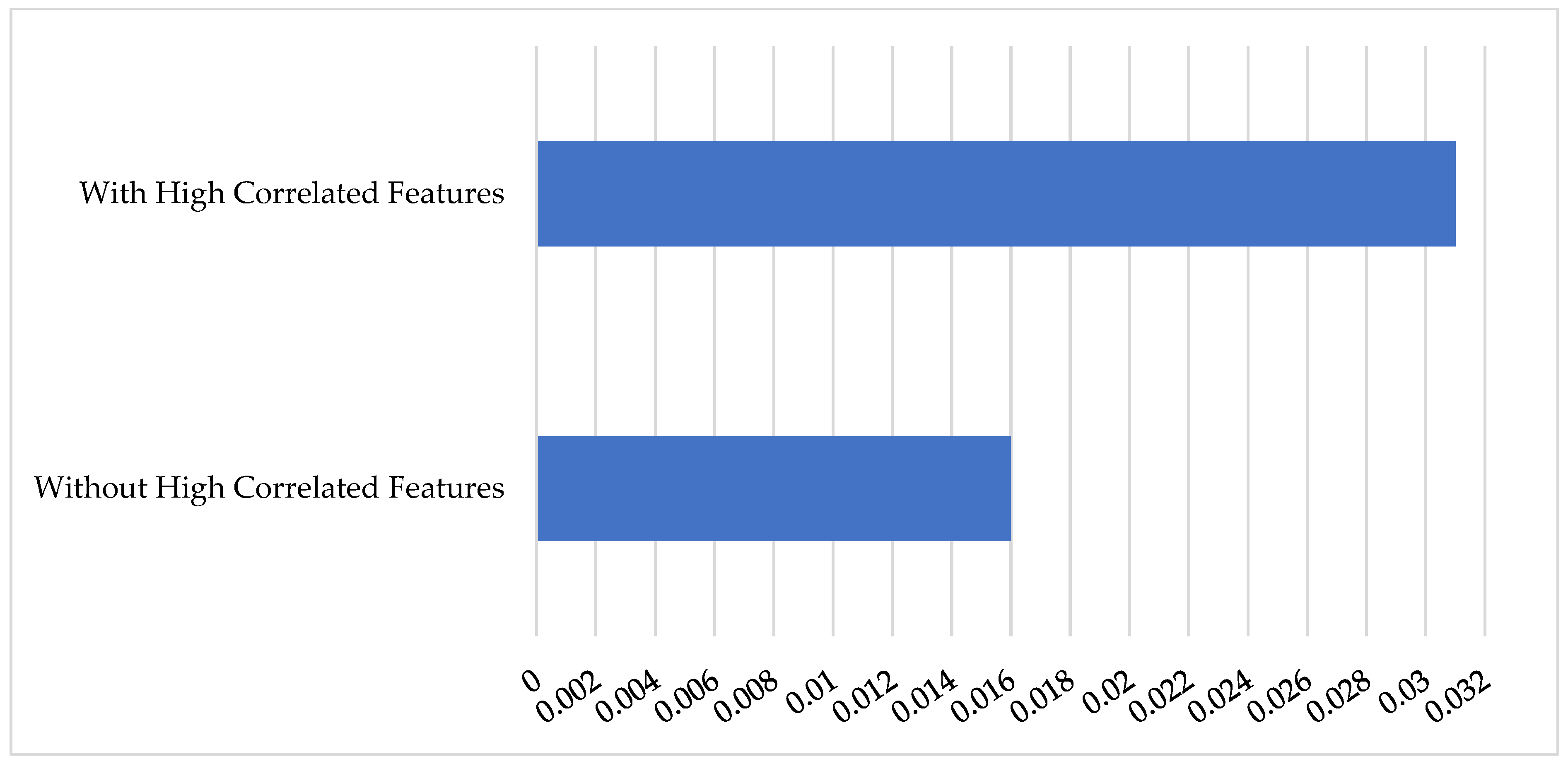
13.	$for i=1:n do$ % Remove highly correlated features
14.	${ pdf}_i\leftarrow \frac{pd{f}_i-\mathrm{m}\mathrm{i}\mathrm{n} \left({pdf}_i\right)}{\max \left({pdf}_i\right)-\mathrm{m}\mathrm{i}\mathrm{n} \left({pdf}_i\right)};$
15.	${\overline{pdf}}_{i\in 1\dots n}\leftarrow \mathrm{R}\mathrm{e}\mathrm{m}\mathrm{o}\mathrm{v}\mathrm{e}\mathrm{H}\mathrm{i}\mathrm{g}\mathrm{h}\mathrm{C}\mathrm{o}\mathrm{r}\mathrm{r}\mathrm{e}\mathrm{l}\mathrm{a}\mathrm{t}\mathrm{e}\mathrm{d}\mathrm{F}\mathrm{e}\mathrm{a}\mathrm{t}\mathrm{u}\mathrm{r}\mathrm{e}\mathrm{s}\left({ pdf}_{i\in 1\dots n}\right)$
16.	Return ${ pdf}_{i\in 1\dots n}$ and ${\overline{pdf}}_{i\in 1\dots n}$
End

3.3.2. Model Building and Training

In this step, the decision-fusion-based model is built by training the three ensemble classifiers described in the previous subsection. The developed model is a meta-model that combines the predictions of GB, XGB, and RF classifiers using a weighted soft-voting rule. The weighted soft-voting rule can produce the score of a class based on the probability score of each classifier multiplied by its weight. The weighted soft-voting rule works well if the combined classifiers solve different problems, such as over-fitting and class-imbalance problems, or the problem that occurs when data have statistical noise [52]. We can calculate the weighted majority voting rule related to the weight $w_i$ of classifier $C_i$ as follows:

$$\widehat{y}=arg \underset{j}{\max } \sum _{i=1}^m{w}_i{f}_j(x)$$

(1)

where $f_j \mathrm{i}\mathrm{s}$ a decision boundary function, written as $f_j\left(x\right)=C_i\left(x\right)=j\in L$, and $L$ is a set of unique labels for classes.

In the case of binary classification for malicious and benign website detection, the class label $j$ ∈ {0, 1} is used, in which class 0 denotes a benign website and 1 a malicious website. Additionally, we assume that the probability classification scores attained by the three ensemble classifiers ($\mathrm{G}\mathrm{B},\mathrm{X}\mathrm{G}\mathrm{B},\mathrm{R}\mathrm{F}$) to classify an example $x$ are:

$$GB(x)=[f_{0,1}, f_{1,1}]$$

(2)

$$XGB(x)=[f_{0,2}, f_{1,2}]$$

(3)

$$RF(x)=[f_{0,3}, f_{1,3}]$$

(4)

By using the weights $w_j$ and the default values of the classifiers’ hyper-parameters, the average probability classification scores are computed as:

$$f\left(l=0,x\right)=f_{0,1}\ast w_1+f_{0,2}\ast w_2+f_{0,3}\ast w_3$$

(5)

$$f\left(l=1,x\right)=f_{1,1}\ast w_1+f_{1,2}\ast w_2+f_{1,3}\ast w_3$$

(6)

$$\widehat{y}=arg \underset{l}{\max } \left[f\left(l=0,x\right), f\left(l=1,x\right)\right]$$

(7)

The value of $\widehat{y}$ is the final classification result of malicious and benign website detection for the proposed DFEL model.

To train and evaluate the DFEL model, holdout and 10-fold cross-validation techniques are used. In the holdout technique, the dataset is randomly divided into two sets: a training set (70%) and test set (30%). The training set is utilized to build the model and the test set is applied to evaluate the model. For the 10-fold cross-validation technique, the dataset is divided into 10 sets, and the model is trained and evaluated in 10 iterations. In each iteration, one set is applied for testing and the other nine sets are used for training. The output of this step is a trained DFEL model.

3.3.3. Data Classification

This step is a part of deployment phase in which the trained model can be used for testing on unseen examples. It depends on the previous supervised learning step. The input is the trained model and the test sets of the holdout and 10-fold cross-validation techniques. The trained model can identify the class of new instances, based on the training data, into “malicious” or “benign” websites. Figure 3 illustrates the data classification step.

In Figure 3, the test instances are pre-processed and classified using GB-, XGB-, and RF-trained classifiers. After that, the classification score of each classifier is weighted using its corresponding weight and summed together with the weighted scores of the other classifiers to form the classification label of the trained DFEL model.

3.3.4. Model Evaluation

The goal of model evaluation is to measure how well the model performs the task. This is an essential step in the development process of machine learning models. Model evaluation can aid in determining the best model that can be represented and its performance in the future. In the training process, evaluating the performance of models in this training set is not acceptable because they can easily produce accurate and over-fitted results. In the machine learning field, there are two techniques for evaluating models: hold-out and the 10-fold cross-validation technique. To avoid over-fitting, both techniques evaluate the model’s performance using an unseen test set.

In the holdout technique, the dataset is randomly divided into training and test sets. The training set is utilized to build models and the test set is used to assess the performance of the developed model. Comprehensively, the 10-fold cross-validation technique is the second evaluation method used to obtain an unbiased estimate of the model performance when there few data are available. The 10-fold cross-validation technique divides the data into 10 sets. Every time, a model is built using nine sets and tested on one set, which is the test set. Model evaluation is performed throughout both experimentation and production.

Some technical metrics, such as accuracy, precision, recall, and F1-socre, are used to evaluate the proposed model across different testing runs, as well as to compare it with different models. These technical metrics are computed based on the classification confusion matrix. In our methodology, the confusion matrix is 2 × 2 for the two classes (malicious, benign). It is generated by the number of correct and incorrect predicted test class values using the classification model in relation to the values of actual test classes. The data in the matrix are widely used to evaluate the performance of such models.

The technical metrics obtained from the confusion matrix can be calculated using the equations given below:

$$Accuracy=\frac{(TP+TN)}{(TP+FP+TN+FN)}$$

(8)

$$Percision=\frac{TP}{(TP+FP)}$$

(9)

$$Recall=\frac{TP}{(TP+FN)}$$

(10)

$$F1-Score=2 \ast \left(\frac{Recall \ast Precision}{Recall+Precision}\right)$$

(11)

where TP, TN, FP, and FN are the true positive, true negative, false positive, and false negative cases, respectively.

As well as the above metrics, the area under curve (AUC) of the receiver operating characteristic (ROC) is used to evaluate the developed model. The AUC is the probability curve in which the degree of separability between classes is given as one of the key evaluation metrics. It measures the classification performance of machine learning models at different threshold values. By using the False Positive Rate (FPR) against True Positive Rate (TPR), the ROC curve can be plotted with a x-axis and y-axis, representing the FPR and TPR, respectively.

4. Experiments and Results

This section validates the proposed approach to detect malicious websites. The approach is able to classify malicious websites and benign ones based on the developed decision-fusion-based ensemble classification model. The experiments can be used to obtain the benchmark dataset and evaluation metrics explained in the previous subsections. Two experiments are conducted to validate the research work. The first experiment is executed using the holdout evaluation, in which two evaluation methods are used: evaluation method one (evaluation method 1) divides the dataset into training set (70%), and test set (30%), and evaluation method two (evaluation method 2) executes the training and validation processes for 15 runs with 15 splits. In each split, the models are trained on a different number of training examples and validated on 10% of the dataset. The second experiment is accomplished using a 10-fold cross-validation technique. The 10-fold cross-validation technique divides the dataset into 10 sets. The training process is conducted for 10 runs. In each run, one set is used to test the base and developed models. In both experiments, the model parameters are initialized, along with their default values. The experiments are implemented using the Python programming language on a laptop with Intel processor Core i7-8750H CPU 2.21 GHz, RAM 32.0 GB and 64-bit Windows 11 operating system.

Before training the ensemble models, we pre-process the dataset using the pre-processing step. We read it and replace the null values with zeroes to make the null values numeric when training the ensemble models. Then, we determine some basic statistics for the dataset to provide an overview of its feature values. Figure 4 shows the uniqueness and frequency of the dataset feature values.

From Figure 4, we can see that the values of the URL feature are totally unique, with very low frequency. This feature can create noise and decrease the accuracy because the difference between them will increase the distance of the model’s decision boundary during the training step. The non-numeric values of features, including the ‘Type’ class label, are also encoded into numbers using label encoding because the classifiers can only learn the numeric values of the features. After that, the correlation between features is analyzed to find highly correlated features. Figure 5 provides a correlation heat map of the dataset features. The correlation heat map is a visual graphical representation of the relationship between features.

Figure 5 demonstrates how each feature is correlated with another feature. It measures the strength of the relationship between every two feature variables. Understanding the correlation between features is useful because the value of one feature can be used to predict the other feature value. The correlated features indicate that, as the value of one feature changes, the other feature tends to change in a specific direction. As shown in Figure 5, the ‘TCP_CONVERSATION_EXCHANGE’, ‘APP_PACKETS’, ‘SOURCE_APP_PACKETS’, ‘REMOTE_APP_PACKETS’, ‘APP_BYTES’, and ‘REMOTE_APP_BYTES’ are highly correlated features with one correlation score. In the next experiment, we will check whether removing these highly correlated features is necessary for a more accurate classification.

4.1. Results of First Experiment

In first experiment, we randomly select a subset of the dataset to test the models. Two evaluation methods are applied to obtain the results of this experiment. The following subsections explain the evaluation methods, along with their outcomes, in detail.

4.1.1. Evaluation Method 1

This evaluation method randomly divides 30% of the dataset to test the models, and the remaining 70% is utilized for training. Figure 6 presents the number of instances of both malicious and benign classes in the training and test sets.

As shown in

Table 2. The distribution of malicious and benign instances in the training and test sets.

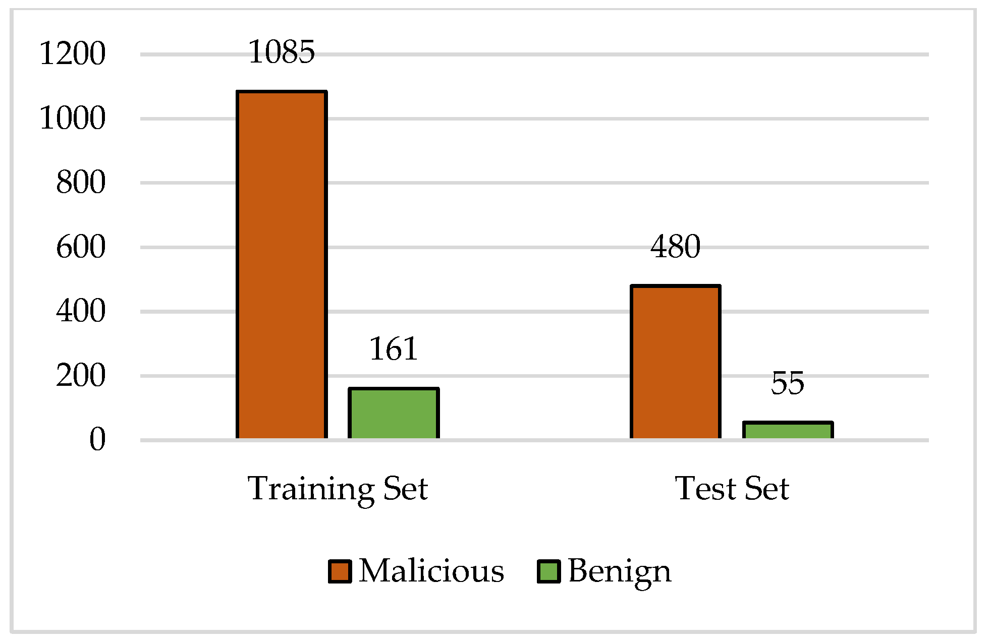
Class Name	Percentage of Training Instances	Percentage of Test Instances
Malicious	87.08%	89.72%
Benign	12.92%	10.28%
Total	100%	100%

, the distribution of instances in the training set is imbalanced, as 87.08% of the total classes are malicious and 12.92% are benign.

After building the DFEL model on the training set without the highly correlated features, it is tested on the test set. Figure 7 displays the confusion matrix of the classification results. The true positive (TP) and true negative (TN) instances are colored with a light green color.

From Figure 7, we can show that the model can correctly classify 477 malicious instances out of 480 and 50 benign instances out of 55. Based on the corrected classified instances,

Table 3. Results of evaluation metrics for a DFEL model trained without high correlated features and tested on a 30% of the dataset.

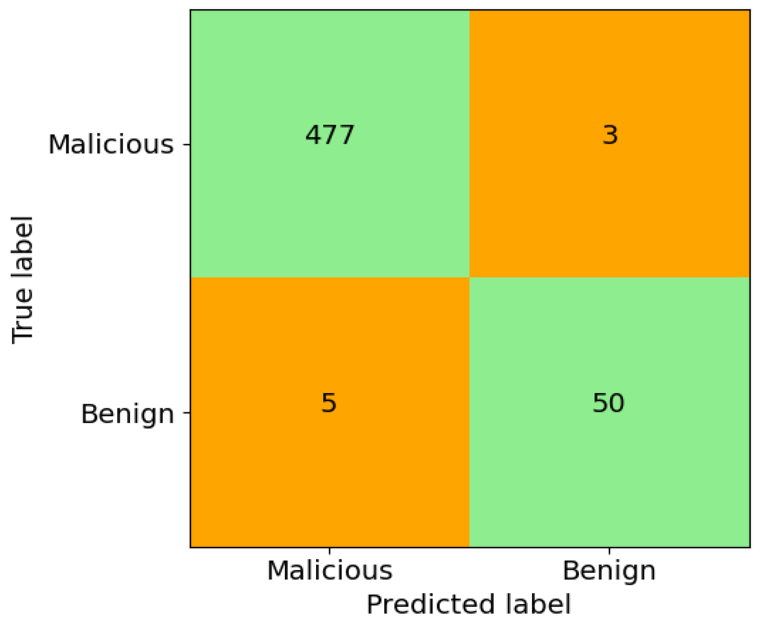
Class Name	Precision	Recall	F1-Score
Malicious	0.9896	0.9938	0.9917
Benign	0.9434	0.9091	0.9259
Macro avg.	0.9665	0.9514	0.9588
Weighted avg.	0.9849	0.9850	0.9849
Accuracy	98.50%

provides the recall, precision, F1-score, and accuracy results for classifying malicious and benign classes.

As shown in Table 3, the proposed model achieves notable classification results, with an accuracy of 98.50%. Since the dataset classes are imbalanced, the accuracy metric is not enough for evaluation; hence, the F1-score is taken as another metric. In Table 3, we can see that the weighted avg. F1-score is 98.49%. The accuracy and F1-score results prove the model’s capability and effectiveness in alleviating the class-imbalanced problem produced by the dominant malicious class label.

To show the effect of highly correlated features, we train the DFEL model on the training set with all features, including the highly correlated features, and test it on the same test set. Figure 8 visualizes the confusion matrix of the classification results. The numbers in the light green color on the confusion matrix are TP and TN instances.

From Figure 8, we can see that the highly correlated features decrease the number of TP instances to 476 instead of 477 to train the model without highly correlated features. The number of TN instances is not affected. The results of other evaluation metrics are given in

Table 4. Results of evaluation metrics for a DFEL model trained with highly correlated features and tested on 30% of the dataset.

Class Name	Precision	Recall	F1-Score
Malicious	0.9896	0.9917	0.9906
Benign	0.9259	0.9091	0.9174
Macro avg.	0.9578	0.9504	0.9540
Weighted avg.	0.9831	0.9832	0.9831
Accuracy	98.32%

.

In Table 4, the model is shown to achieve a classification result with 98.32% accuracy and a 98.31% weighted avg. F1-score. These results confirm that removing the highly correlated features is necessary for a more accurate classification. Moreover, decreasing the number of features increases the efficiency of the model. Figure 9 shows the average classification time of all test sets in seconds for the model trained on the training set with and without highly correlated features.

In Figure 9, we can see that removing highly correlated features decreases the average classification time of all test sets from 0.031 s to 0.016 s, improving the efficiency of the DFEL model in addition to improving the detection accuracy. Moreover, this average classification time confirms the applicability of the proposed model for real-time detection.

Besides, to analyze the ability of the proposed DFEL model compared with its models individually at the 0.5 classification threshold, Figure 10 illustrates the ROC curves of the DFEL model and its other base models.

From Figure 10, we can see that the DFEL model outperforms its base models and achieves a 0.95 AUC, compared with a 0.93, 0.94, and 0.93 AUC for GB, XGB, and RF, respectively. The high AUC value for the DFEL model proves its ability to show how much the trained model can differentiate between test set classes. This means that the built model can classify instances of a malicious class as malicious, and instances of a benign class as benign.

4.1.2. Evaluation Method 2

This evaluation method trains and validates the proposed decision fusion model and its base models 15 times with 15 splits. Each time, the models are trained on a different number of training examples and validated on 10% of the dataset without highly correlated features. Figure 11 demonstrates the learning curves of the DFEL model and its base models. The training and validation scores are compared to the training data examples (data size).

From Figure 11, we can see that when fewer than 600 training examples are used, this not enough to allow the trained models to classify the validation set. In addition, we can see that the training accuracy scores for all models are still around the maximum, and the validation scores increase with more training examples. However, the difference between the accuracy scores for the training and validation of the base models is larger than that of the accuracy scores of the DFEL model for all training sets with more than 600 examples. This means that the performance of the DFEL model is better than its base classifier models.

4.2. Results of Second Experiment

In this experiment, another evaluation experiment is conducted using a 10-fold cross-validation routine to compare the DFEL model with its base models (GB, XGB, and RF).

Table 5. The 10-fold cross-validation averaged accuracy and F1 score results of the GB, XGB, RF, and DFEL models trained on the training folds without highly correlated features.

Model	Averaged F1 Score			Averaged Accuracy
	Micro Avg.	Macro Avg.	Weighted Avg.
GB	0.955	0.888	0.954	95.45%
XGB	0.958	0.895	0.957	95.85%
RF	0.962	0.904	0.960	96.18%
RF + GB	0.958	0.894	0.957	95.79%
GB + XGB	0.963	0.905	0.962	96.29%
RF + XGB	0.967	0.914	0.966	96.74%
Proposed DFEL	0.973	0.931	0.972	97.25%

demonstrates the average accuracy and F1 score of the ten-fold validation results for malicious and benign classification using GB, XGB, RF, and DFEL models trained on training folds without highly correlated features.

As seen in Table 5, the highlighted numbers with bold font are the best evaluation results achieved using a 10-fold cross-validation technique. We can see that the proposed DFEL model outperforms its base models. It can classify the malicious and benign cases with a 97.20% weighted average F1 score and 97.25% average accuracy. In addition, the macro-average F1 scores for each model are less than the micro-average F1 scores because of the class-imbalanced problem. The macro-average F1 score can provide a true evaluation of the classifier model in a class-imbalanced evaluation task.

To confirm whether highly correlated features affect the DFEL’s performance results, we performed 10-fold cross-validation on the training set with highly correlated features. Figure 12 visualizes the 10-fold cross-validation averaged accuracy and F1 score results of the proposed DFEL model trained on the training folds with and without highly correlated features.

From Figure 12, we can see that the DFEL model with highly correlated features attains an average of 96.91% and 96% instead of 97.25% and 97.2% in its 10-fold accuracy and 10-fold weighted average F1 scores, respectively. Moreover, there is a significant difference in the average of the 10-fold macro-averaged F1 scores, in which the model improves the result from 90.4% to 93.1%. These outcomes also confirm that removing highly correlated features is necessary for a more accurate classification.

4.3. Comparison of Results with Related Work

In this subsection, we compared the accuracy of the results of this study with the results of methods and techniques in some recent related studies.

Table 6. Comparison of the results of the accuracy of the proposed DFEL model and the important studies in the literature review.

Authors [Reference]	Year	Methods/Techniques	Accuracy
Amrutkar et al. [29]	2017	kAYO	90%
Sandag et al. [35]	2018	k-NN	95%
McGahagan et al. [30]	2019	AB, ET, RF, GB, BG, LR, and k-NN	89%
Alkhudair et al. [36]	2020	RF	95%
Panischev et al. [37]	2020	RF	95%
Al-milli et al. [32]	2020	1D-CNN	94.31%
Singhal et al. [28]	2020	RF, GB, DT, and DNN	96.4%
Labhsetwar et al. [38]	2021	RF	92%
Singh et al. [39]	2021	Multilayer CNN	91%
Aljabri et al. [40]	2022	NB	96%
Utku and Can [41]	2022	LightGBM, DT, SVM, k-NN, LR, MLP, RF, and XGB	96%
Assefa et al. [34]	2022	Auto-encoder, DT, and SVM	91.24%
Hassan et al. [25]	2022	DT, RF, SVC, LR, and SGD	94.19%
This work	2023	DFEL	98.50%

lists the obtained accuracy result of the proposed DFEL model compared with the accuracies of important studies in the literature review.

As shown in Table 6, our DFEL model results demonstrates a substantial improvement (98.50% vs. 96.4% in terms of accuracy) compared to the results of our recent work. Such a notable performance in terms of website classification provides a possible application of the proposed DFEL model to help cyber-security technicians and researchers in the detection of malicious websites. The other advantage of the decision fusion-based approach is the diversity of GB, XGB, and RF models in reducing the effect of over-fitting and class-imbalanced problems during training development.

5. Conclusions and Future Work

In the cyber-security field, machine-learning-based applications play an essential role in the detection of malicious data, and can also be used to analyze interactive websites and provide efficient solutions. Fusing different data sources and decisions is one of the outstanding strategies to increase the accuracy of machine learning techniques in several applications. This paper proposes an effective and efficient decision-fusion-based approach that fuses the decisions of GB, XGB, and RF classifiers and builds a decision-fusion ensemble learning (DFEL) model. The DFEL is able to classify webpage features and detect the URLs of malicious websites. The final decision is calculated by fusing the classification scores of the three classifiers using a weighted soft-voting method. The outcome could be classified as malicious or benign based on the significant features of the website URLs. An extensive set of experiments is performed on a large public benchmark dataset of malicious and benign website URLs using a 10-fold cross-validation test and different test set ratio. The experimental results show that the proposed fusion method achieved a higher accuracy than the individual models and the current related work. The experimental results also investigate the effect of highly correlated features on the accuracy of the developed model and decrease the detection time by reducing the highly correlated features in the model input. One limitation of this approach is the unavailability of a large class-balanced dataset that can be used to train deep learning models and for malicious websites classification. Consequently, in future work, we will use data-augmentation techniques to extend the size of the minority class in the training set and investigate the advantages of deep learning models on the problem field. Furthermore, we plan to build a model integrated with Fuzzy logic to improve the reliability of the detection approach.

References

- Catal, C.; Ozcan, A.; Donmez, E.; Kasif, A. Analysis of cyber security knowledge gaps based on cyber security body of knowledge. Educ. Inf. Technol. 2023, 28, 1809–1831. [Google Scholar] [CrossRef] [PubMed]
- Gopal, B.; Kuppusamy, P. A comparative study on 4G and 5G technology for wireless applications. IOSR J. Electron. Commun. Eng. 2015, 10, 2278–2834. [Google Scholar]
- Bensberg, F.; Buscher, G.; Czarnecki, C. Digital Transformation and IT Topics in the Consulting Industry: A Labor Market Perspective. In Advances in Consulting Research: Recent Findings Practical Cases; Springer: Berlin/Heidelberg, Germany, 2019; pp. 341–357. [Google Scholar]
- Bayarçelik, E.B.; Bumin Doyduk, H.B. Digitalization of Business Logistics Activities and Future Directions. In Digital Business Strategies in Blockchain Ecosystems: Transformational Design Future of Global Business; Springer: Berlin/Heidelberg, Germany, 2020; pp. 201–238. [Google Scholar]
- Jiang, Y.; Wu, S.; Yang, H.; Luo, H.; Chen, Z.; Yin, S.; Kaynak, O. Secure data transmission and trustworthiness judgement approaches against cyber-physical attacks in an integrated data-driven framework. IEEE Trans. Syst. Man Cybern. Syst. 2022, 52, 7799–7809. [Google Scholar] [CrossRef]
- Mishra, S.; Gochhait, S. Emerging Cybersecurity Attacks in the Era of Digital Transformation. In Proceedings of the 2023 7th International Conference on Intelligent Computing and Control Systems (ICICCS), Madurai, India, 17–19 May 2023; pp. 1442–1447. [Google Scholar]
- Desolda, G.; Ferro, L.S.; Marrella, A.; Catarci, T.; Costabile, M.F. Human factors in phishing attacks: A systematic literature review. ACM Comput. Surv. 2021, 54, 1–35. [Google Scholar] [CrossRef]
- Rupa, C.; Srivastava, G.; Bhattacharya, S.; Reddy, P.; Gadekallu, T.R. A Machine Learning Driven Threat Intelligence System for Malicious URL Detection. In Proceedings of the 16th International Conference on Availability, Reliability and Security, Vienna, Austria, 17–20 August 2021; pp. 1–7. [Google Scholar]
- Aksu, D.; Turgut, Z.; Üstebay, S.; Aydin, M.A. Phishing Analysis of Websites using Classification Techniques. In Proceedings of the International Telecommunications Conference, Istanbul, Turkey, 28–29 December 2017; pp. 251–258. [Google Scholar]
- Vanhoenshoven, F.; Nápoles, G.; Falcon, R.; Vanhoof, K.; Köppen, M. Detecting Malicious URLs using Machine Learning Techniques. In Proceedings of the 2016 IEEE Symposium Series on Computational Intelligence (SSCI), Athens, Greece, 6–9 December 2016; pp. 1–8. [Google Scholar]
- Vanitha, N.; Vinodhini, V. Malicious-URL detection using logistic regression technique. Int. J. Eng. Manag. Res. 2019, 9, 108–113. [Google Scholar]
- Kaddoura, S. Classification of Malicious and Benign Websites by Network Features using Supervised Machine Learning Algorithms. In Proceedings of the 2021 5th Cyber Security in Networking Conference (CSNet), Abu Dhabi, United Arab Emirates, 12–14 October 2021; pp. 36–40. [Google Scholar]
- Odeh, A.; Keshta, I.; Abdelfattah, E. Machine Learningtechniquesfor Detection of Website Phishing: A Review for Promises and Challenges. In Proceedings of the 2021 IEEE 11th Annual Computing and Communication Workshop and Conference (CCWC), Las Vegas, NV, USA, 27–30 January 2021; pp. 0813–0818. [Google Scholar]
- Vijh, M.; Chandola, D.; Tikkiwal, V.A.; Kumar, A. Stock closing price prediction using machine learning techniques. Procedia Comput. Sci. 2020, 167, 599–606. [Google Scholar] [CrossRef]
- Singh, N.; Chaturvedi, S.; Akhter, S. Weather Forecasting using Machine Learning Algorithm. In Proceedings of the 2019 International Conference on Signal Processing and Communication (ICSC), Noida, India, 7–9 March 2019; pp. 171–174. [Google Scholar]
- Chaganti, S.Y.; Nanda, I.; Pandi, K.R.; Prudhvith, T.G.; Kumar, N. Image Classification using SVM and CNN. In Proceedings of the 2020 International Conference on Computer Science, Engineering and Applications (ICCSEA), Gunupur, India, 13–14 March 2020; pp. 1–5. [Google Scholar]
- Zendehboudi, A.; Baseer, M.A.; Saidur, R. Application of support vector machine models for forecasting solar and wind energy resources: A review. J. Clean. Prod. 2018, 199, 272–285. [Google Scholar] [CrossRef]
- Abu Alfeilat, H.A.; Hassanat, A.B.; Lasassmeh, O.; Tarawneh, A.S.; Alhasanat, M.B.; Eyal Salman, H.S.; Prasath, V.S. Effects of distance measure choice on k-nearest neighbor classifier performance: A review. Big Data 2019, 7, 221–248. [Google Scholar] [CrossRef] [PubMed]
- Charbuty, B.; Abdulazeez, A. Classification based on decision tree algorithm for machine learning. J. Appl. Sci. Technol. Trends 2021, 2, 20–28. [Google Scholar] [CrossRef]
- Halimaa, A.; Sundarakantham, K. Machine Learning Based Intrusion Detection System. In Proceedings of the 2019 3rd International Conference on Trends in Electronics and Informatics (ICOEI), Tirunelveli, India, 23–25 April 2019; pp. 916–920. [Google Scholar]
- Christodoulou, E.; Ma, J.; Collins, G.S.; Steyerberg, E.W.; Verbakel, J.Y.; Van Calster, B. A systematic review shows no performance benefit of machine learning over logistic regression for clinical prediction models. J. Clin. Epidemiol. 2019, 110, 12–22. [Google Scholar] [CrossRef]
- Hossin, M.; Sulaiman, M.N. A review on evaluation metrics for data classification evaluations. Int. J. Data Min. Knowl. Manag. Process 2015, 5, 1–11. [Google Scholar]
- Kaur, H.; Pannu, H.S.; Malhi, A.K. A systematic review on imbalanced data challenges in machine learning: Applications and solutions. ACM Comput. Surv. 2019, 52, 1–36. [Google Scholar] [CrossRef]
- Fernández, A.; García, S.; Galar, M.; Prati, R.C.; Krawczyk, B.; Herrera, F. Learning from Imbalanced Data Sets; Springer: Berlin/Heidelberg, Germany, 2018; Volume 10. [Google Scholar]
- Ul Hassan, I.; Ali, R.H.; Ul Abideen, Z.; Khan, T.A.; Kouatly, R. Significance of machine learning for detection of malicious websites on an unbalanced dataset. Digital 2022, 2, 501–519. [Google Scholar] [CrossRef]
- Brandt, J.; Lanzén, E. A Comparative Review of SMOTE and ADASYN in Imbalanced Data Classification; Uppsala Universitet, Statistiska Institutionen: Uppsala, Sweden, 2021. [Google Scholar]
- Teslenko, D.; Sorokina, A.; Khovrat, A.; Huliiev, N.; Kyriy, V. Comparison of Dataset Oversampling Algorithms and Their Applicability to the Categorization Problem. In Innovative Technologies Scientific Solutions for Industries; Kharkiv National University of Radioelectronics: Kharkiv, Ukraine, 2023; pp. 161–171. [Google Scholar]
- Singhal, S.; Chawla, U.; Shorey, R. Machine Learning & Concept Drift Based Approach for Malicious Website Detection. In Proceedings of the 2020 International Conference on COMmunication Systems & NETworkS (COMSNETS), Bengaluru, India, 7–11 January 2020; pp. 582–585. [Google Scholar]
- Amrutkar, C.; Kim, Y.S.; Traynor, P. Detecting mobile malicious webpages in real time. IEEE Trans. Mob. Comput. 2016, 16, 2184–2197. [Google Scholar] [CrossRef]
- McGahagan, J.; Bhansali, D.; Gratian, M.; Cukier, M. A Comprehensive Evaluation of HTTP Header Features for Detecting Malicious Websites. In Proceedings of the 2019 15th European Dependable Computing Conference (EDCC), Naples, Italy, 17–20 September 2019; pp. 75–82. [Google Scholar]
- Patil, D.R.; Patil, J.B. Malicious URLs detection using decision tree classifiers and majority voting technique. Cybern. Inf. Technol. 2018, 18, 11–29. [Google Scholar] [CrossRef]
- Al-Milli, N.; Hammo, B.H. A Convolutional Neural Network Model to Detect Illegitimate URLs. In Proceedings of the 2020 11th International Conference on Information and Communication Systems (ICICS), Irbid, Jordan, 7–9 April 2020; pp. 220–225. [Google Scholar]
- Jayakanthan, N.; Ramani, A.; Ravichandran, M. Two phase classification model to detect malicious URLs. Int. J. Appl. Eng. Res. 2017, 12, 1893–1898. [Google Scholar]
- Assefa, A.; Katarya, R. Intelligent Phishing Website Detection using Deep Learning. In Proceedings of the 2022 8th International Conference on Advanced Computing and Communication Systems (ICACCS), Coimbatore, India, 25–26 March 2022; pp. 1741–1745. [Google Scholar]
- Sandag, G.A.; Leopold, J.; Ong, V.F. Klasifikasi Malicious Websites Menggunakan Algoritma K-NN Berdasarkan Application Layers dan Network Characteristics. CogITo Smart J. 2018, 4, 37–45. [Google Scholar] [CrossRef]
- Alkhudair, F.; Alassaf, M.; Khan, R.U.; Alfarraj, S. Detecting Malicious URL. In Proceedings of the 2020 International Conference on Computing and Information Technology (ICCIT-1441), Tabuk, Saudi Arabia, 9–10 September 2020; pp. 1–5. [Google Scholar]
- Panischev, O.Y.; Ahmedshina, E.N.; Kataseva, D.V.; Katasev, A.; Akhmetvaleev, A. Creation of a fuzzy model for verification of malicious sites based on fuzzy neural networks. Int. J. Eng. Res. Technol. 2020, 13, 4432–4438. [Google Scholar]
- Labhsetwar, S.R.; Kolte, P.A.; Sawant, A.S. Rakshanet: Url-Aware Malicious Website Classifier. In Proceedings of the 2021 2nd International Conference on Secure Cyber Computing and Communications (ICSCCC), Jalandhar, India, 21–23 May 2021; pp. 308–313. [Google Scholar]
- Singh, A.; Roy, P.K. Malicious URL Detection using Multilayer CNN. In Proceedings of the 2021 International Conference on Innovation and Intelligence for Informatics, Computing, and Technologies (3ICT), Zallaq, Bahrain, 29–30 September 2021; pp. 340–345. [Google Scholar]
- Aljabri, M.; Alhaidari, F.; Mohammad, R.M.A.; Mirza, S.; Alhamed, D.H.; Altamimi, H.S.; Chrouf, S.M. An assessment of lexical, network, and content-based features for detecting malicious urls using machine learning and deep learning models. Comput. Intell. Neurosci. 2022, 2022, 3241216. [Google Scholar] [CrossRef]
- Anıl, U.; Ümit, C. Machine Learning-Based Effective Malicious Web Page Detection. Int. J. Inf. Secur. Sci. 2022, 11, 28–39. [Google Scholar]
- Friedman, J.H. Greedy function approximation: A gradient boosting machine. Ann. Stat. 2001, 29, 1189–1232. [Google Scholar] [CrossRef]
- Elith, J.; Leathwick, J.R.; Hastie, T. A working guide to boosted regression trees. J. Anim. Ecol. 2008, 77, 802–813. [Google Scholar] [CrossRef] [PubMed]
- Freund, Y.; Schapire, R.; Abe, N. A short introduction to boosting. J.-Jpn. Soc. Artif. Intell. 1999, 14, 771–780. [Google Scholar]
- Khalilia, M.; Chakraborty, S.; Popescu, M. Predicting disease risks from highly imbalanced data using random forest. BMC Med. Inform. Decis. Mak. 2011, 11, 51. [Google Scholar] [CrossRef]
- Teramoto, R. Balanced gradient boosting from imbalanced data for clinical outcome prediction. Stat. Appl. Genet. Mol. Biol. 2009, 8, 20. [Google Scholar] [CrossRef]
- Chen, T.; He, T.; Benesty, M.; Khotilovich, V.; Tang, Y.; Cho, H.; Chen, K.; Mitchell, R.; Cano, I.; Zhou, T. Xgboost: Extreme gradient boosting. R Package Version 0.4-2 2015, 1, 1–4. [Google Scholar]
- González, S.; García, S.; Del Ser, J.; Rokach, L.; Herrera, F. A practical tutorial on bagging and boosting based ensembles for machine learning: Algorithms, software tools, performance study, practical perspectives and opportunities. Inf. Fusion 2020, 64, 205–237. [Google Scholar] [CrossRef]
- Bentéjac, C.; Csörgő, A.; Martínez-Muñoz, G. A comparative analysis of gradient boosting algorithms. Artif. Intell. Rev. 2021, 54, 1937–1967. [Google Scholar] [CrossRef]
- Zhang, L.; Suganthan, P.N. Random forests with ensemble of feature spaces. Pattern Recognit. 2014, 47, 3429–3437. [Google Scholar] [CrossRef]
- Biau, G.; Scornet, E. A random forest guided tour. TEST 2016, 25, 197–227. [Google Scholar] [CrossRef]
- Karlos, S.; Kostopoulos, G.; Kotsiantis, S. A Soft-Voting Ensemble Based Co-Training Scheme Using Static Selection for Binary Classification Problems. Algorithms 2020, 13, 26. [Google Scholar] [CrossRef]